Lattice Hamiltonian approach to the Schwinger model: further results from the strong coupling expansion

Abstract:

We employ exact diagonalization with strong coupling expansion to the massless and massive Schwinger model. New results are presented for the ground state energy and scalar mass gap in the massless model, which improve the precision to nearly $10^{-9}\%$. We also investigate the chiral condensate and compare our calculations to previous results available in the literature. Oscillations of the chiral condensate which are present while increasing the expansion order are also studied and are shown to be directly linked to the presence of flux loops in the system.

1 Introduction

The Schwinger model [1], i.e. QED in 1+1 dimensions, has become a toy model for gauge theories. It is simple enough to analytically extract its behavior in various limits [2], but it still exhibits such interesting phenomena as chiral symmetry breaking and quark confinement [3].

The model has been studied thoroughly using various methods [2]–[11]. Recently, we were able to show that the Hamiltonian approach still can give results that are comparable or sometimes exceed the precision of other methods [5]. In this article, we continue that study by showing updated results and expand it to another observable – the chiral order parameter (chiral condensate).

The outline of this paper is as follows. In Section 2 we shortly recall the Schwinger model and Section 3 describes the method we use – exact diagonalization with strong coupling expansion. Our results, a comparison to previous findings and a thorough description of chiral condensate oscillations are included in Section 4, which is then followed by Section 5 – the summary.

2 The Schwinger model

The Hamiltonian of the massive Schwinger model on lattice, in the Kogut-Susskind discretization [12, 13] and after the Jordan-Wigner transformation [14] to the spin space is :

$$\hat{\mathcal{H}}=\frac{1}{2a}\sum_{n=1}^{M}\left(\sigma^{+}(n)e^{i\theta(n)}\sigma^{-}(n+1)+\text{h.c.}\right)+\frac{m}{2}\sum_{n=1}^{M}(1+(-1)^{n}\sigma^{3}(n))+\frac{g^{2}a}{2}\sum_{n=1}^{M}L^{2}(n),$$ (1)

where $a$ – lattice spacing, $m$ – fermion mass, $g$ – coupling, $M$ – system size. $\sigma^{i}(n)$ are Pauli matrices operating in spin space, $L(n)$ is related to electric field $L(n)=E(n)/g$ and operates in ladder space $L|l\rangle=l|l\rangle,l=0,\pm 1,\pm 2,\ldots$, and $e^{\pm i\theta(n)}$ are rising and lowering operators in this ladder space.

We will be interested in assessing the chiral condensate $\Sigma$, which is given by:

$$\frac{\Sigma}{g}=\frac{\sqrt{x}}{2M}\langle 0|\sum_{n=1}^{M}(-1)^{n}\sigma^{3}(n)|0\rangle,$$ (2)

where $|0\rangle$ is the ground state of the Hamiltonian and $x=\frac{1}{a^{2}g^{2}}$. The theoretical prediction for the massless model is $\Sigma/g|_{m=0}=-e^{\gamma}/{2\pi^{3/2}}\approx-0.1599288$.

3 Method

The Hamiltonian (1) can be rewritten in the dimensionless form as:

$$\hat{W}=\frac{2}{ag^{2}}\hat{\mathcal{H}}=\hat{W}_{0}+x\hat{V}$$ (3)

with $\hat{W}_{0}$ including the mass part and the electric field part and $\hat{V}$ including the hopping. If $x$ is small (strong coupling), then we can treat $\hat{W}_{0}$ as an unperturbed Hamiltonian and $\hat{V}$ as a perturbation.

We employ the exact diagonalization (ED) approach with the strong coupling expansion (SCE) introduced by Hamer [15] and initially used for the Schwinger model in Refs. [2, 3]. SCE truncates the Hamiltonian, by selecting only those states that are connected with the ground state up to a specific order of perturbation. Then, the truncated Hamiltonian is finite and thus amenable to ED.

In Ref. [5] we suggested to use a very high order $N$ of SCE, for which the eigenvalues are saturated, i.e. do not change when further increasing $N$, up to machine precision. The saturation was present for observables such as ground state energy and scalar/vector mass gaps for the massless model. The same method will be used to determine another observable – the chiral condensate.

4 Results and comparison

4.1 Ground state energy and scalar mass gap

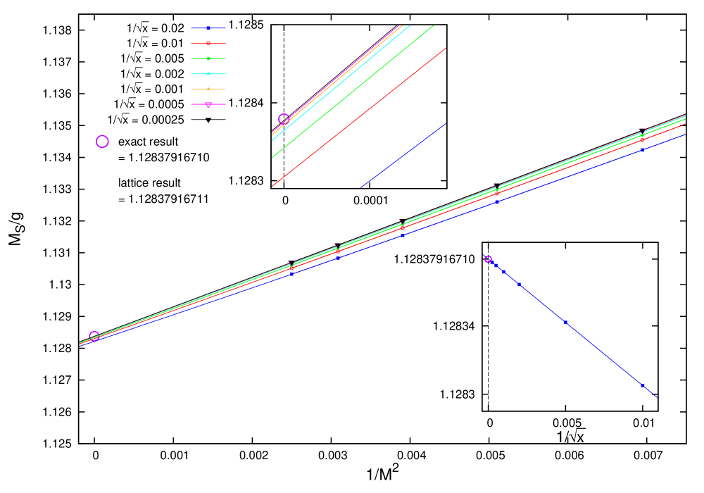
Figure 1: Infinite volume extrapolation ($M\rightarrow\infty$) of the scalar mass gap. Top inset shows a zoomed in view. Bottom inset shows the continuum extrapolation ($1/\sqrt{x}\to 0$).

First, we present updated results for the ground state energy $E_{0}$ and scalar mass gap $M_{S}/g$ for the massless Schwinger model, obtained by increasing the maximal system size (with respect to Ref. [5]) and thus being able to get closer to the continuum limit (increase maximal $x$). We show the continuum limit extrapolation of the scalar mass gap in Fig. 1, while Tab. 1 presents the comparison to our previous result, which shows significant improvement.

Observable	$E_{0}$	(error)	$M_{S}/g$	(error)
Previous calculation [5]	$-0.3183098827$	$1.1\cdot 10^{-6}\%$	$-1.1283791668$	$2.9\cdot 10^{-8}\%$
This work	$-0.3183098860$	$6.5\cdot 10^{-8}\%$	$-1.12837916711$	$1.3\cdot 10^{-9}\%$
Exact value	$-0.3183098862$	$-$	$-1.12837916710$	$-$

Table 1: Comparison with previous results [5] for ground state energy $E_{0}$ and scalar mass gap $M_{S}/g$.

4.2 Chiral condensate

Our results for the chiral condensate in the massless case are summarized in Fig. 2. The inset shows an example of our infinite volume extrapolation, using an exponential ansatz normally expected for periodic boundary conditions away from the critical point ($x\rightarrow\infty$). The results in infinite volume are then shown in the main plot and used to extrapolate to the continuum limit. It can be shown even in the free theory that the approach to the continuum limit is linear in the lattice spacing with logarithmic corrections (and higher-order corrections). In the plot, we show such fit and compare it to the purely linear one. Indeed, the correct result in the continuum limit is obtained only if the logarithmic corrections are taken into account.

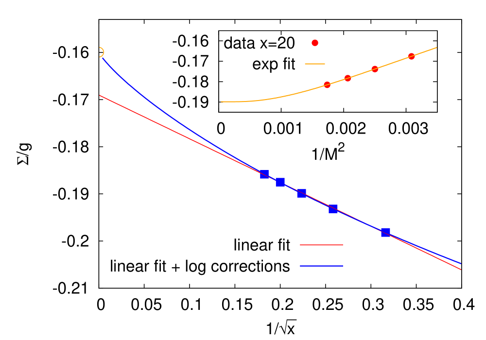
Figure 2: Chiral condensate for the massless case – continuum limit estimation. Inset shows an example of the infinite volume limit estimation for $x=20$ with exponential fit.

$x$	$m/g$	SCE+ED	MPS [7]	Difference
20	0	$-0.189879$	$-0.190253$	0.000374
25	0	$-0.187519$	$-0.187969$	0.000450
30	0	$-0.185830$	$-0.186208$	0.000378
cont.	0	$-0.1600(17)$	$-0.159930(8)$
cont.	0.125	$-0.0906(23)$	$-0.092023(4)$

Table 2: Comparison of SCE+ED and MPS results [7] for the chiral condensate in the massless and massive ($m/g=0.125$) model. For the massive model, a logarithmic divergence had to be subtracted.

The comparison with Matrix Product States (MPS) results [7] is shown in Tab. 2. Interestingly, the infinite volume limit values for SCE+ED are always a bit smaller than those for MPS. This might suggest that our exponential fitting function is subject to power-law corrections that dominate the behavior close to the continuum limit (cf. infinite volume scaling for the scalar mass gap – Fig. 1). The continuum limit result is in agreement with MPS, but it has much lower accuracy, due to the fact that MPS allows to study much larger system sizes and much larger values of $x$.

The massive case was also investigated, where a logarithmic divergence has to be subtracted (this divergence is present already in the free case). The fermion mass tends to increase finite volume effects. Once again, though our findings are consistent with previous work, they have much less precision.

4.3 Oscillations of the chiral condensate

4.3.1 Description of the oscillations

When one starts increasing the SCE order $N$, for some values of $x$ a problem appears with estimating the saturated values. Examples are shown in Fig. 3. We can clearly see that for small values of $x$ (away from the continuum limit), oscillations are very small, almost non-existent. However, when we approach the continuum limit and thus $x$ is very big, the oscillations are clearly visible and we cannot directly extract the saturated value.

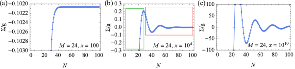
Figure 3: Chiral condensate when increasing the SCE order $N$ for different couplings: (a) $x=10^{2}$, (b) $x=10^{4}$, (c) $x=10^{10}$. On plot (b) we can see a tail, marked in green and oscillations, marked in red.

Interestingly, the plots show two distinct regions: the tail at $N\lesssim M$ and the oscillations which have a very specific period. For now, we will ignore the tail part and try to describe the oscillations by fitting them to a chosen function. Our ansatz includes an oscillating part (sine), a modulation (decreasing function of $N$) and a constant shift (saturated value of $\Sigma$). It was found that the modulation part can be best described as a function of $\frac{1}{N^{3}}$ for large $x$ and as an inverse exponential function of $N$ for small $x$. Thus, the final fitting function is:

$$\Sigma(N)/g=\Sigma(N\rightarrow\infty)/g+a\left(\frac{b}{N^{3}}+e^{-\alpha N}\right)\sin\left(\frac{2\pi}{T}N+\varphi\right),$$ (4)

where $\Sigma(N\rightarrow\infty)/g,a,b,\alpha,T$ and $\varphi$ are the fitting parameters. The data was always fitted starting from the second extremum of $\Sigma(N)/g$, so that the effects of the tail part are greatly diminished.

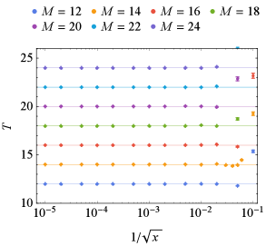
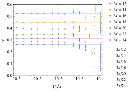
Figure 4: Period (left) and phase (right) of oscillations. The lines on the $T$ plot indicate $T=12,14,\ldots,24$.

The period and the phase of oscillations are shown in Fig. 4. We can clearly see that close to the continuum limit (large $x$), we have the following dependencies:

$$T=M,\hskip 10.00002pt\varphi=\frac{2\pi}{M}.$$ (5)

However, these equations seem to be invalid for small $x$. This is due to the fact that for small $x$ the oscillations are too small to be well-described by our ansatz. On the phase $\varphi$ plot, we can see that errors grow for small $x$, which also indicates this problem.

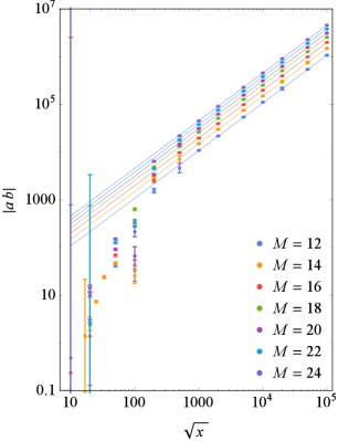
Figure 5: Coefficient in front of $\frac{1}{N^{3}}$. The solid lines are the linear fits to $y=ax$ function, which on the log-log will always be parallel to each other.

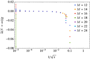
Figure 6: Saturated values of the chiral condensate, $\Sigma(N\rightarrow\infty)/g$. Notice that the naive extrapolation to the continuum limit would yield $\Sigma/g\rightarrow 0$.

The coefficient in front of $\frac{1}{N^{3}}$ was also investigated and it is shown in Fig. 6. We are taking the absolute value of the coefficient, due to the sine function being antisymmetric ($\sin x=-\sin(-x)$). The data seems to indicate that this coefficient is proportional to $\sqrt{x}$:

$$|ab|=A(M)\cdot\sqrt{x}.$$ (6)

However, on the log-log plot we can clearly see that for small $x$, this dependence is again invalid.

Fig. 6 shows saturated values of the chiral condensate obtained from fitting of the oscillations. Interestingly, for a very large $x(\sim 10^{10})$, there are very big errors present – this is due to huge amplitude of oscillations.

It would seem that the continuum limit value $\Sigma(M\rightarrow\infty,x\rightarrow\infty)/g$ is zero. However, this invalid result is obtained due to large finite volume effects: we firstly have to take the infinite volume limit which is quite problematic with our approach, if we work too close to the continuum limit. Only after taking the infinite volume limit, we can take the continuum limit by fitting the infinite volume limit data and extracting the $x\rightarrow\infty$ value.

4.3.2 Final fitting ansatz

Using relationships extracted in section 4.3.1, we can rewrite the final fitting ansatz as:

$$\Sigma(N,M,x)/g=\Sigma(N\rightarrow\infty,M,x)/g+\left(A(M)\frac{\sqrt{x}}{N^{3}}+B(M,x)e^{-\alpha(M,x)N}\right)\sin\frac{2\pi}{M}(N+1).$$ (7)

We can immediately see that for $N=kM-1$ the sine function will reach the middle point of oscillations. So, if there is any residual function that we omitted in our fitting ansatz, it will be present at those points. Therefore, we suggest to use values for $N=kM-1$ to extract the saturated value of the chiral condensate by fitting those specific plot points.

4.3.3 Connection to the number of flux loops in the system

Every time $N=kM,k\in\mathbbm{Z}$, states generated in the SCE procedure will include the next positive $(L(n)=+1,+2,+3,\ldots)$ and the next negative $(L(n)=-1,-2,-3,\ldots)$ flux loop in the system. For example, for $N=2M$, the Hamiltonian will include flux loops $L(n)=-2,-1,+1,+2$. Thus, we can see that the value for SCE order $N$ must be very close to the value for SCE order $N+M$, because both systems have very similar structure except for the number of included flux loops. We therefore conclude that the period of the oscillations being a constant $M$ is a manifestation of the flux loops in the system.

Now, we can also see that the physical interpretation of the tails in Fig. 3 is the absence of the flux loops in the Hamiltonian, which is true for $N<M$.

5 Summary and outlook

We presented updated results for the ground state energy and scalar mass gap for the massless Schwinger model. The precision of scalar mass gap calculation was increased up to almost $10^{-9}\%$, which, to our knowledge, is the most precise lattice result ever obtained. It is, however, of minor practical importance, because it can not be systematically extended to other observables or non-zero fermion mass. As such, it should be considered an interesting peculiarity of the spectrum of the massless case.

We have also shown findings for the chiral condensate for both massless and massive model. Our results indicate large finite volume effects that make it impossible to achieve lattice spacings as small as when using the MPS method. Note, however, that the lattice spacings that can be used are still much smaller than when using standard Monte Carlo methods (where typically $\beta\equiv x\leq 10$).

Finally, we have described our findings concerning chiral condensate oscillations when increasing the SCE order and we have shown that they can be directly linked to the number of flux loops in the system.

References

- [1] J. Schwinger, Phys. Rev., 128 (1962) 2425–2429.
- [2] D.P. Crewther, C.J. Hamer, Nucl. Phys. B, 170 (1980) 353–368.
- [3] C.J. Hamer, J. Kogut, D.P. Crewther, M.M. Mazzolini, Nucl. Phys. B, 208 (1982) 413–438.
- [4] T. Byrnes, P. Sriganesh, R. Bursill, C. Hamer, Phys. Rev. D, 66 (2002) 13002 [hep-lat/0202014].
- [5] K. Cichy, A. Kujawa-Cichy, M. Szyniszewski, Comput. Phys. Commun., 184 (2013) 1666–1672 [hep-lat/1211.6393].
- [6] M.C. Bañuls, K. Cichy, J.I. Cirac, K. Jansen, JHEP, 11 (2013) 158 [hep-lat/1305.3765].
- [7] M.C. Bañuls, K. Cichy, J.I. Cirac, K. Jansen, H. Saito, PoS(Lattice 2013) (2013) 332 [hep-lat/1310.4118].
- [8] E. Rico, T. Pichler, M. Dalmonte, P. Zoller and S. Montangero, Phys. Rev. Lett., 112 (2014) 201601 [cond-mat.quant-gas/1312.3127].
- [9] B. Buyens, J. Haegeman, K. Van Acoleyen, H. Verschelde and F. Verstraete, Phys. Rev. Lett., 113 (2014) 091601 [hep-lat/1312.6654].
- [10] Y. Shimizu and Y. Kuramashi, Phys. Rev. D, 90 (2014) 014508 [hep-lat/1403.0642].
- [11] H. Saito, M.C. Bañuls, K. Cichy, J.I. Cirac, K. Jansen, PoS(Lattice 2014) (2014) 302.
- [12] J. Kogut, L. Susskind, Phys. Rev. D, 11 (1975) 395.
- [13] T. Banks, L. Susskind, J. Kogut, Phys. Rev. D, 13 (1976) 1043–1053.
- [14] P. Jordan, E. Wigner, Z. Phys., 47 (1928) 631–651.
- [15] C.J. Hamer, Phys. Lett. B, 82 (1979) 75–78.