Preparation of edge states by shaking boundaries

Abstract

Preparing topological states of quantum matter, such as edge states, is one of the most important directions in condensed matter physics. In this work, we present a proposal to prepare edge states in Aubry-Andr$\acute{\textrm{e}}$-Harper (AAH) model with open boundaries, which takes advantage of Lyapunov control to design operations. We show that edge states can be obtained with almost arbitrary initial states. A numerical optimalization for the control is performed and the dependence of control process on the system size is discussed. The merit of this proposal is that the shaking exerts only on the boundaries of the model. As a by-product, a topological entangled state is achieved by elaborately designing the shaking scheme.

I introduction

Topological insulators(TIs) hasan10 ; qi11 are new states of quantum matter with profound physical features that have their origin in topology. They have a bulk insulating gap but are distinct from ordinary insulators at stable gapless edge states. The quantum Hall systemthouless82 , which is an insulator without any kind of spontaneous symmetry breaking, is the first example of topological insulators.

It is believed that there only exists topological trivial phase in 1D systems due to the lack of symmetries. Recently, it has been shown that the 1D quasiperiodic system YEK1109 shares the same topological non-trivial phase emerged in the 2D integer quantum Hall effect DRH-PRB14 . Indeed, the edge state that characterizes topological property in this system has been observed YEK1109 . Most recently, topologically protected edge state has been demonstrated in the 1D commensurate off-diagonal Aubry-Andr$\acute{\textrm{e}}$-Harper (AAH) model SA-AIPS3 , interpreted by the $\textrm{Z}_{2}$ topological index of the Kitaev model AYK-PU44 . It is worth noticing that the topology properties have been studied in optical lattices extensively hormozi12 ; degottardi13 ; satija13 ; cooper12 ; price12 ; kjall12 ; atala13 ; zhu13 ; grusdt13 ; deng13 ; NG-PRL105 ; TDS-PRA82 ; BB-PRL107 ; JK-PRL111 ; ganeshan13 , and the edge states have been observed in the photonic system TK1105 ; MH1302 .

State steering is an important task in quantum control. Many protocols DD2007 have been proposed for this purpose, including the optimal control technique, adiabatic control, the technique of stimulated Raman scattering involving adiabatic passage (STIRAP), and open loop controls based on Lyapunov functions. Among them, the Lyapunov based control has its own advantages due to the effectiveness designing for control fields. To apply the Lyapunov control, a function called Lyapunov function has to be specified first. Then the control fields can be designed by guaranteeing the decrease of Lyapunov function, and the system would evolve to the target state asymptotically. In particular, this control scheme has been studied by several researchers KB-SCL56 ; SK-A44 ; XXY-PRA80 ; XTW-PRA80 ; JMC-NJP11 ; WW-PRA82 ; XTW-IEEE55 ; SCH-PRA86 and has been applied to diverse fields in physics.

In this paper, we steer an arbitrary given initial state into the edge states in a 1D optical lattice by only shaking the on-site energy of the boundaries, which can be established via the Lyapunov control. By choosing different Lyapunov functions, we show distinct convergence behaviors for the system. In addition, we also explore a feasible way to realize boundary-boundary entangled states LCV-PRA76 ; SID-JETP85 ; LB-PRA82 .

The paper is organized as follows. In Sec. II, we present a general formalism for the Lyapunov control. In Sec. III, we first apply the general method to steer the system into edge state by shaking only the energy of boundary sites, and study the dynamical behaviors with different Lyapunov functions. Then we show how to optimize the Lyapunov function in terms of fidelity and control time. An exploration on the effect of errors on the fidelity of final state is given in Sec. IV. By use of the elaborate designing control fields, we study the behavior of boundary-boundary entangled states in Sec. V. Finally, we conclude in Sec. VI.

II Lyapunov control

Although the problem of quantum control might be formulated in different ways, the final purpose is mostly to steer a quantum system from an (arbitrary) initial state to a target state by control fields. We start with the dynamics of a quantum system governed by Schrödinger equation ($\hbar=1$)

$$|\dot{\psi}(t)\rangle = -i[H_{0}+\sum_{k}f_{k}(t)H_{k}]|\psi(t)\rangle,$$ (1)

where $H_{0}$ and $H_{k}$ denote the system Hamiltonian and control Hamiltonian, respectively. $f_{k}(t)$ represent the control fields. As mentioned in the introduction, the design of the control fields can be different from proposal to proposal. Here, we use the Lyapunov control technique to design the control fields. The essence of the Lyapunov control is to choose a Lyapunov function, which is required to be positive and reaches its minimum when the system arrives at target state. Obviously, the following form of Lyapunov function

$$V_{1}=1-|\langle\psi_{T}|\psi(t)\rangle|^{2},$$ (2)

meets the requirement. Here $|\psi_{T}\rangle$ denotes the target state which is conventionally an eigenstate of system Hamiltonian. The time derivative of $V_{1}$ yields

$$\dot{V}_{1}=-2\sum_{k}|\langle\psi(t)|\psi_{T}\rangle|f_{k}(t)\textrm{{Im}}[e^{i\arg\langle\psi(t)|\psi_{T}\rangle}\langle\psi_{T}|H_{k}|\psi(t)\rangle],$$ (3)

where $\textrm{{Im}}[\cdot]$ stands for the imaginary part of $[\cdot]$ and $\textrm{arg}\langle\psi(t)|\psi_{T}\rangle$ is the angle between states $|\psi(t)\rangle$ and $|\psi_{T}\rangle$. Thus, the condition $\dot{V}_{1}\leq 0$ can be satisfied naturally if we choose the control fields $f_{k}(t)=A_{1k}\textrm{{Im}}[e^{i\arg\langle\psi(t)|\psi_{T}\rangle}\langle\psi_{T}|H_{k}|\psi(t)\rangle]$ with $A_{1k}>0$. Especially, $A_{1k}$ can be used to adjust the amplitude of control fields and the control time.

As the Lyapunov function is not unique, it can be constructed differently even though the control problem is same. For example, we may define another Lyapunov function by

$$V_{2}=\langle\psi(t)|P|\psi(t)\rangle,$$ (4)

where the operator $P$ is hermitian and time independent. Additionally, $P$ is also assumed to be positive semidefinite operator acting on the Hilbert space spanned by the eigenvectors of the system Hamiltonian $H_{0}$. With this definition, the time derivative of $V_{2}$ becomes

$$\dot{V}_{2} = \langle\psi(t)|i[H_{0},P]|\psi(t)\rangle+\sum_{k}f_{k}(t)\langle\psi(t)|i[H_{k},P]|\psi(t)\rangle.$$ (5)

The Lyapunov control requires that the operator $P$ should be constructed properly to guarantee XXY-PRA80

$$[H_{0},P]=0.$$ (6)

Therefore a straightforward way to construct the operator $P$ is

$$P=p_{f}|\lambda_{f}\rangle\langle\lambda_{f}|+\sum_{i\neq f}p_{i}|\lambda_{i}\rangle\langle\lambda_{i}|,$$ (7)

where $|\lambda_{i}\rangle$ ($i=1,...,N$) are the eigenstates of system Hamiltonian with corresponding eigenvalues $\lambda_{i}$, and $|\lambda_{f}\rangle$ is the target state. Of course, the values of $p_{f}$ and $p_{i}$ ($i=1,...,N,i\neq f$) can be chosen arbitrarily except for the necessary condition $p_{f}<p_{i}$XXY-PRA80 . Clearly, if we select the control fields $f_{k}(t)=-A_{2k}\langle\psi(t)|i[H_{k},P]|\psi(t)\rangle$ with $A_{2k}>0$, the condition $\dot{V}_{2}\leq 0$ is satisfied naturally. Discussions on the Lyapunov function are in order. The Lyapunov function given in equation (4) with equation (7) is quite general for unitary systems. In fact, the Lyapunov function $V_{2}$ covers the Lyapunov function $V_{1}$ note2 . This suggests that the optimalization over the Lyapunov function reduces to searching a set of $\{p_{j}\}$ that maximizes the fidelity of final state or minimizes the control time, etc., depending on the optimal function. We will carry out this optimalization latter.

According to the Lyapunov control theory, the Lyapunov function $V_{k}$ will converge to its minimum while the state of system converges to a LaSalle’s invariant set given by $\mathcal{E}_{k}=\{\dot{V_{k}}=0\}$ ($k=1,2$). When the dimension of LaSalle’s invariant space is more than one, it becomes complicate to control a quantum system from an arbitrary initial state to a given target state. Nonetheless, by elaborately designing the Lyapunov function, we can still steer a quantum system to evolve into a desired state.

III Preparation of edge state in AAH model

The system of interest is the Fermi gas loaded in a 1D optical lattice, where the system Hamiltonian reads

$$H_{0}=-t\sum_{i=1}^{N-1}(c_{i}^{{\dagger}}c_{i+1}+h.c.)+V\sum_{i=1}^{N}\cos(2\pi\alpha i+\delta)c_{i}^{{\dagger}}c_{i}.$$ (8)

Here $N$ is the total number of optical lattice sites. $t$ is the hopping amplitude between the $i$-th and $(i+1)$-th site and set to be the unit of energy throughout this paper. $c_{i}$ and $c_{i}^{{\dagger}}$ are the fermionic annihilation and creation operators for the $i$-th site, respectively. $V$ denotes the strength of commensurate potential with an rational number $\alpha$. When $\alpha$ is an irrational number, $V$ represents the strength of incommensurate potential which is the well-known Aubry-Andr$\acute{\textrm{e}}$ model SA-AIPS3 , namely, all eigenstates are extended (localized) for $V<2$ ($V>2$) with a single excitation.

Under open boundary condition with proper parameters, there exist edge states $\{|\texttt{Edge}_{i}\rangle\}$ locating near boundary sites, which stems from the non-trivial properties of the system and can be envisioned by mapping to the 2D quantum Hall effects in the Hofstadter problem YEK1109 ; LJL-PRL108 . Especially, in the single excitation subspace, eigenstates localized near boundaries can be found by resolving the eigenvalue equation,

$$H_{0}|\lambda_{i}\rangle=\lambda_{i}|\lambda_{i}\rangle,i=1,...,N,$$ (9)

where the $i$-th single particle eigenstate is given by $|\lambda_{i}\rangle=\sum_{j}^{N}b_{j,i}c_{j}^{{\dagger}}|0\rangle$. $b_{j,i}$ are the superposition coefficients and satisfy the normalization condition $\sum_{j}^{N}|b_{j,i}|^{2}=1$. Figure 1 demonstrates the probability distribution of two edge states. Remarkably, the amplitude of edge states mainly locate at the boundary sites.

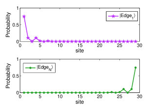
Figure 1: (a) The probability amplitude of each site in edge state $|\texttt{Edge}_{1}\rangle$. (b) The probability amplitude of each site in edge state $|\texttt{Edge}_{N}\rangle$. $|\texttt{Edge}_{1}\rangle$ ($|\texttt{Edge}_{N}\rangle$) denotes the edge state that the amplitude dominantly occupies at site $1$ ($N$). We study in the single excitation subspace and other parameters are chosen as $N$=29, $\alpha=1/3$, $V=1.5$, $\delta=2\pi/3$.

Next we explore how to use Lyapunov control to steer this system into one of two edge states. Note that one of the key points in the control process is how to choose a proper control Hamiltonian. If the structure of control Hamiltonian is much complex, even though it can be used to achieve edge states in theory, it may be difficult to manipulate in experiments. On the contrary, it may not steer the system into edge states when the control Hamiltonian is too simple. After combining with the feature of edge states, we find it is sufficient to prepare edge states by modulating the on-site energy of boundaries, which can be implemented easily. The control Hamiltonian then can be written as

$$H_{1}=c_{1}^{{\dagger}}c_{1},~{}~{}~{}H_{2}=c_{N}^{{\dagger}}c_{N},$$ (10)

and the Lyapunov function can be chosen as

$$V_{1}=1-|\langle\psi_{T}|\psi(t)\rangle|^{2},$$ (11)

which results in the control fields $f_{k}(t)=A_{1k}\textrm{{Im}}[e^{i\arg\langle\psi(t)|\psi_{T}\rangle}\langle\psi_{T}|H_{k}|\psi(t)\rangle].$ To be specific, we consider $A_{1k}=1$ in numerical calculations, and our goal is to steer an arbitrary given initial state to one of the edge states, for instance, $|\psi_{T}\rangle=|\texttt{Edge}_{N}\rangle$.

One can find from equation (2) or (4) that the Lyapunov functions are time dependent via $|\psi(t)\rangle$, which implies that the control fields would depend on the initial state at the beginning. So, to design the control fields, we have to know the initial state $|\psi_{0}\rangle$, though it might be arbitrary. As the single particle states (i.e., the single excitation occupies only at site $n$, denoted by $|n\rangle(n=1,...,N)$) are more easily to prepare, we consider these states as initial states in the following. Note that this method can also be applied for arbitrary superposition of the single particle states. Figure 2 shows the time evolution of the fidelity defined by $F_{\psi(t)\texttt{Edge}_{N}}=|\langle\psi(t)|\texttt{Edge}_{N}\rangle|$ and the control fields $f_{k}(t)$ while the initial state of system is chosen as $|\psi_{0}\rangle=|3\rangle$. We find that the control fields $f_{k}(t)$ can steer the initial state to the edge state eventually. In addition to this, it can also be observed that the control field $f_{2}(t)$ plays an important role in the evolution, since the control field $f_{1}(t)$ is comparatively small. The physics behinds this result can be understood as follow. The excitation mainly occupies at site $N$ for the target state $|\texttt{Edge}_{N}\rangle$, thus the control Hamiltonian $H_{2}$ dominates during the time evolution. As a result, the corresponding control field plays an important role.

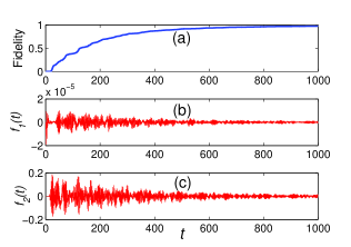
Figure 2: (a) The time evolution of fidelity $F_{\psi(t)\texttt{Edge}_{N}}$. All parameters are in units of the hopping amplitude $t$. (b) The time dependence of the control field $f_{1}(t)$. (c) The time dependence of the control field $f_{2}(t)$.

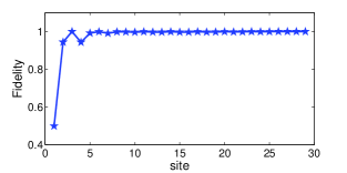
Figure 3: The fidelity $F_{\psi_{s}\texttt{Edge}_{N}}$ versus different initial states, $|\psi_{0}\rangle=|n\rangle~{}(n=1,...N)$. The other parameters are the same as in figure 2.

Next, we investigate the fidelity $F_{\psi_{s}\texttt{Edge}_{N}}$ (denotes the fidelity between the final state $|\psi_{s}\rangle$ and the target state $|\texttt{Edge}_{N}\rangle$) at different initial states $|\psi_{0}\rangle=|n\rangle(n=1,...,N)$, which are illustrated in figure 3. There is an intuitive hypothesis from figure 3 that the fidelity $F_{\psi_{s}\texttt{Edge}_{N}}$ might be related to the fidelity $F_{\psi_{0}\texttt{Edge}_{1}}$ (denotes the fidelity between the initial state $|\psi_{0}\rangle$ and the edge state $|\texttt{Edge}_{1}\rangle$). In order to confirm it, figure 4(a) demonstrates the relation between the fidelity $F_{\psi_{s}\texttt{Edge}_{N}}$ and the fidelity $F_{\psi_{0}\texttt{Edge}_{1}}$. We can see in figure 4(a) that steering the system to the target state becomes much difficult with the increasing of $F_{\psi_{0}\texttt{Edge}_{1}}$, since the edge state $|\texttt{Edge}_{1}\rangle$ is also an element of the LaSalle’s invariant set (we will demonstrate it in the following). Therefore, small value of $F_{\psi_{0}\texttt{Edge}_{1}}$ benefits the control process when we set the edge state $|\texttt{Edge}_{N}\rangle$ as the target state. This observation also holds true when the initial state is an arbitrary superposition of the single particle states, which is not shown in figure 4(a). Those results can be explained as follow. As the initial state can be rewritten as a superposition of the eigenstates of the system Hamiltonian $H_{0}$, i.e.,

$$|\psi_{0}\rangle=a(0)|\texttt{Edge}_{1}\rangle+\sum_{i=2}^{N}a_{i}(0)|\lambda_{i}\rangle.$$ (12)

Since the edge state $|\texttt{Edge}_{1}\rangle$ is an element of the largest invariant set, the amplitude of the edge state $|\texttt{Edge}_{1}\rangle$ remains almost unchanged during the control process and the other eigenstates would be steered into the target state. Consequently, it can not be steered into the target state perfectly if the initial state contains the component of the edge state $|\texttt{Edge}_{1}\rangle$. The details of proof can be found in the appendix.

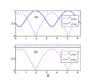
Figure 4: $F_{\psi_{s}\texttt{Edge}_{N}}$ and $F_{\psi_{0}\texttt{Edge}_{1}}$ as a function of $\theta\in[0,2\pi]$ with (a) Lyapunov function $V_{1}$ and (b) Lyapunov function $V_{2}$. The initial state is chosen as $|\psi_{0}\rangle=\cos{\theta}|1\rangle+\sin{\theta}|2\rangle$ because the amplitude of the edge state $|\texttt{Edge}_{1}\rangle$ mainly locates at site 1 and site 2.

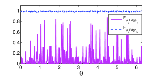
Figure 5: $F_{\psi_{s}\texttt{Edge}_{N}}$ (blue line) and $F_{\psi_{0}\texttt{Edge}_{1}}$ (pink line) as a function of parameter $\theta$ with Lyapunov function $V_{2}$ and operator $P_{1}$. The initial state is $|\psi_{0}\rangle=\cos{\theta}|n\rangle+\sin{\theta}|m\rangle$, where $n,m$ are stochastic integer created between 1 and $N$, while $\theta$ $\in[0,2\pi]$, $N=29$. The results are a collection of 500 random initial states.

As the choice of Lyapunov function is not unique, we can choose another Lyapunov function to design the control fields for the system, which we have elucidated in Sec. II. Based on several trials, we choose the operator $P$ as

$$P_{1}=p_{f}|\texttt{Edge}_{N}\rangle\langle\texttt{Edge}_{N}|+\sum_{i\neq f}p_{i}|\lambda_{i}\rangle\langle\lambda_{i}|,$$ (13)

where $p_{i}=\lambda_{i}$ and $p_{f}=-3$ guarantee $p_{f}<p_{i}$. The corresponding control fields are specified as $f_{k}(t)=-A_{2k}^{1}\langle\psi(t)|i[H_{k},P_{1}]|\psi(t)\rangle$ with $A_{2k}^{1}=5$. From figure 4(b), we observe that a high fidelity of final state can be obtained with an (almost) arbitrarily given initial state by elaborately designing the value of $p_{i}$ ($i=1,...,N$) in equation (7) note . More generally, figure 5 shows a collection of fidelity with an arbitrary given initial state in the form $|\psi_{0}\rangle=\cos{\theta}|n\rangle+\sin{\theta}|m\rangle$, and we find that it can approach 98.74% on average. Here $n$ and $m$ in the initial states are integers stochastically created from 1 to $N$. This observation argues that the value of $F_{\psi_{0}\texttt{Edge}_{1}}$ has slightly effects on the fidelity of final state when the operator $P$ is elaborately constructed.

The above numerical calculations imply that different Lyapunov functions lead to different fidelity and behaviors of convergence due to the distinct largest invariant set. To be more specific, The largest invariant set with Lyapunov function $V_{1}$ is $\mathcal{E}_{1}=\{|\psi\rangle,\ \ |\langle\psi_{T}|H_{k}|\psi\rangle=0,k=1,2\}$ while it is $\mathcal{E}_{2}=\{|\psi\rangle,\ \ |\langle\lambda_{i}|H_{k}|\lambda_{j}\rangle\langle\lambda_{j}|\psi\rangle\langle\psi|\lambda_{i}\rangle=0,k=1,2;~{}i,j=1,...,N\}$ for the Lyapunov function $V_{2}$ SK-A44 . It can be verified easily that only the state $|\texttt{Edge}_{N}\rangle$ belongs to the largest invariant set when designing by the Lyapunov function $V_{2}$ and the hermitian operator $P_{1}$. Nevertheless, this is not the case for the Lyapunov function $V_{1}$. There exists another solution $|\psi\rangle=|\texttt{Edge}_{1}\rangle$ that satisfies the condition $\langle\psi_{T}|H_{k}|\psi\rangle=0(k=1,2)$, thus the largest invariant set $\mathcal{E}_{1}$ is spanned by $\{|\texttt{Edge}_{1}\rangle,|\texttt{Edge}_{N}\rangle\}$. This enlarged invariant set caused by the Lyapunov function $V_{1}$ makes the control behaviors different from that of Lyapunov function $V_{2}$. As a consequence, the control with the Lyapunov function $V_{1}$ may not steer the system to the target state very well. From this point of view, it is important to choose a proper Lyapunov function in order to obtain a high fidelity of the target state.

Since there are many ways to choose Lyapunov functions as aforementioned, it gives rise to a question: how to optimize the Lyapunov function in order to obtain a high fidelity of final state. In the following, we analyze and answer this question. The Lyapunov function is required to be real and positive, so it can be written as an average of hermitian operator $P$. Therefore, the Lyapunov function in equation (4) is general form. By the principle of Lyapunov control, control fields must vanish and Lyapunov function should reach its minimum when the system arrives at the target state. This requires that the operator $P$ must commute with the system Hamiltonian $H_{0}$ (see equation (5)). Hence the general form of operator $P$ takes,

$$P=p_{0}\cdot\mathcal{I}+\sum_{i}^{N}p_{i}|\lambda_{i}\rangle\langle\lambda_{i}|,$$ (14)

where $|\lambda_{i}\rangle$ ($i=1,...,N$) are the eigenstates of system Hamiltonian and $p_{i}(i=0,...,N)$ are arbitrary real numbers.

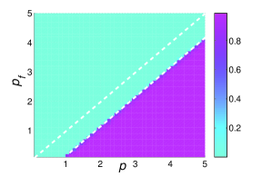
Figure 6: The fidelity of final state to the edge state $|\texttt{Edge}_{N}\rangle$ as a function of coefficients $p$ and $p_{f}$. We have chosen the initial state $|\psi_{0}\rangle=|3\rangle$, the control time $t=1000$, and the Lyapunov function $V_{2}$ with the operator $P_{1}$.

With these considerations, the optimalization over the Lyapunov function reduces to searching a set of $\{p_{i}\}$ that maximize the fidelity of final state. Note that the term with identity operator $\mathcal{I}$ is a constant when substituting $P$ into equation (4). It does not affect the designing for control fields, as a consequence, $p_{0}$ can be an arbitrary value. To simplify the optimalization scheme, we assume $p_{i}=p$ $(i\neq f)$, and the optimalization is furthermore simplified to analyze the relationship between the fidelity and the coefficients $p$ and $p_{f}$ with a fixed control time. It should be addressed that the optimalization should be taken over all $p_{i}$ ($i=1,...,N$), but it is a consuming task when $N$ is large, so here we simplify the problem and use the simple case to exemplify the optimalization scheme. Figure 6 shows the fidelity of final state as a function of $p_{f}$ and $p$. We find that it fails to prepare the edge state when $p_{f}>p$ since the final state is not the target state when the Lyapunov function $V_{2}$ reaches its minimum. We can also see that the fidelity of final state is almost unchanged with $p-p_{f}>1$ and vanishes with $p-p_{f}<1$. The reason can be found in figure 7, which shows the relation between the control time and $p_{f}$, where the control process is completed when the fidelity of final state reaches 0.97 with $p=5$. For $p-p_{f}<1$, it takes a long time to have such a fidelity. In other words, the fidelity of final state is very small if the control time stops at $t=1000$. In addition, we find from figure 7 that the control time almost stays at a fixed value for $p-p_{f}>1$, which provides us with a guidance for designing the coefficients in the Lyapunov function.

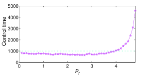
Figure 7: The control time as a function of $p_{f}$ (pink line with stars) while the fidelity reaches 0.97 and we have fixed $p=5$. The other parameters are the same as in figure 6.

IV robustness

In practise, there inevitably exist some errors during the control process. For example, it requires to know the initial state precisely, but the preparation of initial state may not be perfect. Errors may also occur in the application of control fields. In the following, we investigate the effect of these errors on the fidelity of final state, which are characterized by $\delta$. Namely, if the theoretical exact values of control fields are $f_{k}(t)$, the actual control fields applied in the control process are $f^{\prime}_{k}(t)=(1+\delta)f_{k}(t)$. As to errors in the initial state, we randomly create a state, and mix it with the initial state (e.g., $|3\rangle$) such that $\delta=1-|\langle\psi_{0}|3\rangle|$, where $|\psi_{0}\rangle$ is the actual initial state and $|3\rangle$ is the ideal initial state. With these considerations, we simulate the influence of errors on the fidelity of final state in figure 8. It can be found that the unperfect preparation of initial state $|3\rangle$ does not have a serious effect on the fidelity of final state. The control field $f_{1}(t)$ has a slight influence on the fidelity of final state, but the control field $f_{2}(t)$ does affect the fidelity of final state. The reason is that the edge state $|\texttt{Edge}_{N}\rangle$ is mainly localized at the site $N$ in the optical lattice, then the control field $f_{2}(t)$ dominates in the control process.

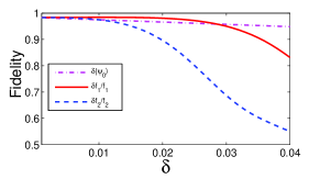
Figure 8: We have assumed that the perfect initial state is $|3\rangle$, where the errors caused by unperfect preparation is defined by $\delta=1-|\langle\psi_{0}|3\rangle|$. The red solid line and blue dash line shows the fidelity of final state versus the errors caused by mismatching control fields $f_{1}(t)$ and $f_{2}(t)$ respectively. The other parameters are the same as in figure 6.

On the other hand, it can be found in figure 9(a) that different initial states manifest distinct dynamics behaviors and convergence time in the control process since the Lyapunov functions rely on the initial state $|\psi_{0}\rangle$ through $|\psi(t)\rangle$. In addition, the total lattice sites can also affect the control time and the time for edge state preparation is approximate linearly proportional to the total lattice sites, as shown in figure 9(b).

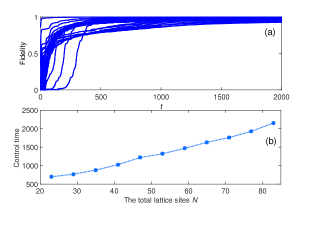
Figure 9: (a) The dynamics evolution of fidelity with different initial states $|\psi_{0}\rangle=|n\rangle,~{}~{}n=1,...,N$. The Lyapunov function is $V_{2}$ with the operator $P_{1}$. (b) The control time versus different total lattice sites $N$ when the fidelity is 0.99, where the initial state is $|3\rangle$.

V Boundary-boundary entangled states

For the system under Lyapunov control, we have shown that the LaSalle’s invariant set is spanned by $\{|\texttt{Edge}_{1}\rangle,|\texttt{Edge}_{N}\rangle\}$ for Lyapunov function $V_{1}$. As a result the state of the system would asymptotically converge to

$$|\psi(t)\rangle=\alpha|\texttt{Edge}_{1}\rangle+\beta|\texttt{Edge}_{N}\rangle.$$ (15)

Equivalently, it can be rewritten as

$$|\psi(t)\rangle=\sum_{n=1}^{N}C_{n}(t)|n\rangle,$$ (16)

where $C_{n}(t)$ represents the probability amplitude of a single particle located at the $n$-th site in the optical lattice. In order to get a high degree of boundary-boundary entangled states, we deform the Lyapunov function as

$$V_{3}=1-|\langle\texttt{Edge}_{1}|\psi(t)\rangle|^{2}-|\langle\texttt{Edge}_{N}|\psi(t)\rangle|^{2},$$ (17)

and the time derivative of $V_{3}$ yields

$$\dot{V}_{3}=-2\sum_{k=1,2}f_{k}(t)\sum_{m=1,N}|\langle\psi(t)|\texttt{Edge}_{m}\rangle|\textrm{{Im}}[e^{i\arg{\langle\psi(t)|\texttt{Edge}_{m}\rangle}}\langle\texttt{Edge}_{m}|H_{k}|\psi(t)\rangle].$$ (18)

Hence, the control field can be chosen as $f_{k}(t)=-A_{3k}\sum_{m=1,N}\textrm{{Im}}[e^{i\arg\langle\psi(t)|\texttt{Edge}_{m}\rangle}\langle\texttt{Edge}_{m}|H_{k}|\psi(t)\rangle]$ with $A_{3k}=1$.

When investigating the entanglement between site $1$ and site $N$ in the optical lattice, the remaining sites should be traced out, i.e., $\rho_{1N}(t)=\textrm{Tr}_{2...N-1}(|\psi(t)\rangle\langle\psi(t)|)$. In the Hilbert space spanned by $\{|00\rangle,|10\rangle,|01\rangle,|11\rangle\}$, we have the following expression for reduced density matrix $\rho_{1N}(t)$

$${\rho_{1N}(t)}=\left(\begin{array}[]{cccc}a&0&0&0\\ 0&b&d&0\\ 0&d^{*}&c&0\\ 0&0&0&0\\ \end{array}\right)$$ (19)

with $a=\sum_{n=2}^{n=N-1}|C_{n}|^{2}$, $b=|C_{1}|^{2}$, $c=|C_{N}|^{2}$, $d=C_{1}C_{N}^{*}$. Then we use concurrence WKW-PRL80 to measure the degree of entanglement,

$$\mathcal{C}(\rho)\equiv\max\{0,\lambda_{1}-\lambda_{2}-\lambda_{3}-\lambda_{4}\},$$ (20)

where $\lambda_{l}~{}(l=1,2,3,4)$ are the square roots of eigenvalues of the matrix $\rho(\sigma_{y}\otimes\sigma_{y})\rho^{\ast}(\sigma_{y}\otimes\sigma_{y})$ in decreasing order, and $\rho^{\ast}$ is the complex conjugate of $\rho$. According to the expression of ${\rho_{1N}}(t)$, it is straightforward to find that

$$\mathcal{C}_{1N}=\max\{0,2\sqrt{bc},2|d|\}.$$ (21)

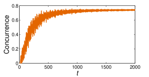
Figure 10: The concurrence $\mathcal{C}_{1N}$ as a function of time $t$, where Lyapunov function is $V_{3}$.

Figure 10 illustrates the dynamics behavior of concurrence with initial state $|\psi_{0}\rangle=|3\rangle$, which shows that the concurrence $\mathcal{C}_{1N}$ approaches to a fixed value 0.74. It should be noted that the entanglement of steady state depends on the initial state, in particular it is very closely connected to the fidelity $F_{\psi_{0}\texttt{Edge}_{1}}$ between the initial state and the edge state $|\texttt{Edge}_{1}\rangle$, which is shown in figure 11. Additionally, it is readily found that the average value of concurrence reaches about 0.71 in numerical calculations. The reason why the concurrence of steady entangled state is below 0.75 can be found as follow. As we have shown, the final state is approximate a superposition of two edge states and the probability amplitudes of edge states on the first and end site are about 0.7474 in figure 1. When $\alpha=\beta=\frac{1}{\sqrt{2}}$ in equation (15), the entanglement of edge states reaches its maximum, which helps to establish the concurrence of boundary-boundary entangled state. Although the boundary-boundary entanglement is not very high, it is symmetry protected and therefore maybe useful in quantum information processing (actually, it is almost a maximal entanglement between two edge states).

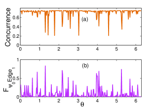
Figure 11: (a) The concurrence $\mathcal{C}_{1N}$ and (b) the fidelity $F_{\psi_{0}\texttt{Edge}_{1}}$ as a function of initial states characterized by the parameter $\theta$, where Lyapunov function is $V_{3}$, $\theta\in[0,2\pi]$. The initial state is $|\psi_{0}\rangle=\cos{\theta}|n\rangle+\sin{\theta}|m\rangle$, where $n,m$ are stochastic integer ranging from 1 to $N$. We simulate the concurrence and fidelity with 300 random initial states.

VI conclusion

In conclusion, we have proposed a scheme to prepare edge states in the optical lattice by shaking boundaries, which is motivated by the fact that the edge states exhibit interesting physical properties. The control Hamiltonian we use is restricted to the boundaries of the optical lattice and the control field is designed by Lyapunov control where the Lyapunov function lies at the heart of control design. By choosing different Lyapunov functions, we have shown that the control process would lead to different fidelity and convergence feature. It have been found that the edge state we obtain depends on the initial states with Lyapunov function $V_{1}$ while it can be obtained for almost arbitrary initial states when using Lyapunov function $V_{2}$ with operator $P_{1}$. In addition, we have discussed the influence of errors on the fidelity of edge state. By this proposal, we can also prepare boundary-boundary entangled state which is actually the maximum superposition of two edge states.

This work is supported by the National Natural Science Foundation of China (Grants No. 11534002, No. 61475033 and 11475037), and supported by the Fundamental Research Funds for the Central Universities under grant No. DUT15LK26.

APPENDIX

In this appendix, we show that the amplitude of edge state $|\texttt{Egde}_{1}\rangle$ almost remains unchanged under the control with Lyapunov function $V_{1}$. In the following, we adopt the same notions as those in the main text.

Suppose the initial state of this system is

$$|\psi_{0}\rangle = a(0)|\texttt{Edge}_{1}\rangle+\sum_{i=2}^{N}a_{i}(0)|\lambda_{i}\rangle.$$ (22)

The state at time $t$ becomes

$$|\psi(t)\rangle=a(t)|\texttt{Edge}_{1}\rangle+\sum_{i=2}^{N}a_{i}(t)|\lambda_{i}\rangle.$$ (23)

According to the Schrödinger equation, we can deduce the differential equation for the probability amplitude of edge state $|\texttt{Egde}_{1}\rangle$ ($\hbar=1$),

$$i\cdot\dot{a}(t) = \langle\texttt{Edge}_{1}|[H_{0}+\sum_{k=1}^{2}f_{k}(t)H_{k}]|\psi(t)\rangle$$ (24)

$$= \lambda_{1}\cdot a(t)+\gamma_{1}\cdot a(t)+\sum_{j=2}^{N}\gamma_{j}\cdot a_{j}(t),$$

where $\gamma_{j}=\langle\texttt{Edge}_{1}|[f_{1}(t)H_{1}+f_{2}(t)H_{2}]|\lambda_{j}\rangle,~{}j=2,...,N.$

On the other hand, since the edge state $|\texttt{Egde}_{N}\rangle$ locates near at site $N$, the probability amplitude of edge state $|\texttt{Egde}_{N}\rangle$ on the site $1$ almost vanishes, i.e., $\epsilon\ll 1$ (the magnitude order $\epsilon\sim 10^{-5}$ in the case of $N=29$). It is similar to the situation of edge state $|\texttt{Egde}_{1}\rangle$. Thus one can estimate the order of magnitude in $H_{1}|\texttt{Egde}_{N}\rangle$ and $H_{2}|\texttt{Egde}_{1}\rangle$:

$$H_{1}|\texttt{Egde}_{N}\rangle = H_{1}|\psi_{T}\rangle\sim\epsilon\cdot(1,\underbrace{0,...,0}_{N-1})^{T},$$

$$H_{2}|\texttt{Egde}_{1}\rangle \sim \epsilon\cdot(\underbrace{0,...,0}_{N-1},1)^{T},$$ (25)

where the superscript $T$ represents transposition and the order of magnitude in the function $f_{1}(t)$ can be estimated as well:

$$f_{1}(t)=\texttt{{Im}}[e^{i\textrm{arg}\langle\psi(t)|\psi_{T}\rangle}\langle\psi_{T}|H_{1}|\psi(t)\rangle]\sim\epsilon.$$ (26)

Those estimations give the order of magnitude in $\gamma_{j}$:

$$|\gamma_{j}| = |f_{1}(t)\langle\texttt{Egde}_{1}|H_{1}|\lambda_{j}\rangle+f_{2}(t)\langle\texttt{Egde}_{1}|H_{2}|\lambda_{j}\rangle|\sim\epsilon\ll|\lambda_{1}|.$$ (27)

Therefore the differential equation of $a(t)$ can be approximated as

$$i\cdot\dot{a}(t)\simeq\lambda_{1}\cdot a(t),$$ (28)

leading to

$$|a(t)|^{2}\simeq constant=|a(0)|^{2}.$$ (29)

Hence, the amplitude of edge state $|\texttt{Egde}_{1}\rangle$ almost remains unchanged during the control process with Lyapunov function $V_{1}$.

References

- (1) M. Z. Hasan and C. L. Kane, Rev. Mod. Phys. 82, 3045 (2010).
- (2) X. L. Qi and S. C. Zhang, Rev. Mod. Phys. 83, 1057 (2011).
- (3) D. J. Thouless, M. Kohmoto, M. P. Nightingale, and M. den Nijs, Phys. Rev. Lett. 49, 405 (1982).
- (4) Y. E. Kraus, Y. Lahini, Z. Ringel, M. Verbin, and O. Zilberberg, Phys. Rev. Lett. 109, 106402 (2012)
- (5) D. R. Hofstadter, Phys. Rev. B 14, 2239 (1976).
- (6) S. Aubry and G. Andr, Ann. Isr. Phys. Soc. 3, 133 (1980).
- (7) A. Y. Kitaev, Phys.-Usp. 44, 131 (2001).
- (8) S. Ganeshan, K. Sun, and S. Das Sarma, Phys. Rev. Lett. 110, 180403 (2013).
- (9) I. I. Satija and G. G. Naumis, Phys. Rev. B 88, 054204 (2013).
- (10) W. DeGottardi, D. Sen, and S. Vishveshwara, Phys. Rev. Lett. 110, 146404 (2013).
- (11) L. Hormozi, G. Möller, and S. H. Simon, Phys. Rev. Lett. 108, 256809 (2012).
- (12) N. R. Cooper and R. Moessner, Phys. Rev. Lett. 109, 215302 (2012).
- (13) H. M. Price and N. R. Cooper, Phys. Rev. A 85, 033620 (2012).
- (14) J. A. Kjäll and J. E. Moore, Phys. Rev. B 85, 235137 (2012).
- (15) M. Atala, M. Aidelsburger, J. T. Barreiro, D. Abanin, T. Kitagawa, E. Demler, and I. Bloch, Nat. Phys. 9, 795 (2013).
- (16) S. L. Zhu, Z. D.Wang, Y. H. Chan, and L. M. Duan, Phys. Rev. Lett. 110, 075303 (2013).
- (17) F. Grusdt, M. Höning, and M. Fleischhauer, Phys. Rev. Lett. 110, 260405 (2013).
- (18) X. Deng and L. Santos, Phys. Rev. A 89, 033632 (2014).
- (19) N. Goldman, I. Satija, P. Nikolic, A. Bermudez, M. A. M. Delgado, M. Lewenstein, and I. B. Spielman, Phys. Rev. Lett. 105, 255302 (2010).
- (20) T. D. Stanescu, V. Galitski, and S. Das Sarma, Phys. Rev. A 82, 013608 (2010).
- (21) B. Bri and N. R. Cooper, Phys. Rev. Lett. 107, 145301 (2011).
- (22) J. Klinovaja and D. Loss, Phys. Rev. Lett. 111, 196401 (2013).
- (23) T. Kitagawa, M. A. Broome, A. Fedrizzi, M. S. Rudner, E. Berg, I. Kassal, A. Aspuru-Guzik, E. Demler, and A. G. White, Nat. Comm. 3, 882, (2012).
- (24) M. Hafezi, J. Fan, A. Migdall, and J. M. Taylor, Nat. Photon. 7, 1001 (2013).
- (25) D. D’Alessandro, Introduction to Quantum Control and Dynamics (Taylor and Francis Group, Boca Raton, 2007).
- (26) K. Beauchard, J. M. Coron, M. Mirrahimi, and P. Rouchon, Systems and Control Letters. 56, 388 (2007).
- (27) S. Kuang and S. Cong, Automatica 44, 98 (2008).
- (28) X. X. Yi, X. L. Huang, C. F. Wu and C. H. Oh, Phys. Rev. A 80, 052316 (2009)
- (29) X. T. Wang and S. G. Schirmer, Phys. Rev. A 80, 042305 (2009).
- (30) J. M. Coron, A. Grigoriu, C. Lefter, and G. Turinici, New J. Phys. 11, 105034 (2009).
- (31) W. Wang, L. C. Wang, and X. X. Yi, Phys. Rev. A 82, 034308 (2010)
- (32) X. T. Wang and S. G. Schirmer, IEEE Transactions on Automatic Control 55, 2259 (2010).
- (33) S. C. Hou, M. A. Khan, X. X. Yi, D. Y. Dong, and I. R. Petersen, Phys. Rev. A 86, 022321 (2012).
- (34) L. C. Venuti, S. M. Giampaolo, F. Illuminati, and P. Zanardi, Phys. Rev. A 76, 052328 (2007).
- (35) S. I. Doronin, A. N. Pyrkov, and . B. Fel’dman, JETP Lett. 85, 519 (2007).
- (36) L. Banchi, T. J. G. Apollaro, A. Cuccoli, R. Vaia, and P. Verrucchi, Phys. Rev. A 82, 052321 (2010).
- (37) We get in equation (2) by taking in equation (4), where is the identity operator.
- (38) L. J. Lang, X. M. Cai, and S. Chen, Phys. Rev. Lett. 108, 220401 (2012).
- (39) The Lyapunov control can not steer a system from an initial state in the LaSalle’s invariant set to the target state.
- (40) W. K. Wootters, Phys. Rev. Lett. 80, 2245 (1998).