Quantum decoherence of an anharmonic oscillator monitored by a Bose-Einstein condensate

Abstract

The dynamics of a quantum anharmonic oscillator whose position is monitored by a Bose-Einstein condensate (BEC) trapped in a symmetric double well potential is studied. The (non-exponential) decoherence induced on the oscillator by the measuring device is analysed. A detailed quasiclassical and quantum analysis is presented. In the first case, for an arbitrary initial coherent state, two different decoherence regimes are observed: An initial Gaussian decay followed by a power law decay for longer times. The characteristic time scales of both regimes are reported. Analytical approximated expressions are obtained in the full quantum case where algebraic time decay of decoherence is observed.

I Introduction

Recent experiments Hunger et al. (2010); Treutlein et al. (2012) show that a great degree of coherent control is possible between micromechanical oscillators and a Bose-Einstein condensate (BEC) of magnetically trapped Rubidium-87 atoms Reichel et al. (2001). Chip-based magneto traps offer a high degree of control when the BEC and a micromechanical cantilever are brought close to distances of the order of the micrometer. At that level of proximity between a cantilever and a BEC, the surface forces start to play a role. Such forces allow one to couple coherently the collective dynamics of a condensate and a mechanical oscillator. Accordingly, it is possible to study the interaction between trapped atoms and on-chip-solid-state systems such as nano-micro mechanical oscillators Schwab and Roukes (2005); Kippenberg and Vahala (2008); Treutlein et al. (2007).

One of the major experimental goals is to use neutral atoms to coherently manipulate the state of the oscillator. There are several proposals aimed at achieving this by employing atoms in a cavity with a moving mirror Meiser and Meystre (2006); Genes et al. (2008); Ian et al. (2008), or by coupling atoms by means of a reflective membrane, where the lattice trapping the atoms is built by reflecting a laser beam off the membrane Camerer et al. (2011); Vogell et al. (2013).

Such opto-mechanical systems, composed by nano-mechanical oscillators and atoms interfaced via optical quantum buses, have been recently discussed in the context of quantum non-demolition Bell measurements and the ability to prepare EPR entangled states Hammerer et al. (2009). Also ions are proposed as transducers for electromechanical oscillators Hensinger et al. (2005) while other proposals involve the coupling between oscillators and dipolar molecules Singh et al. (2008). A growing interest, both theoretical and experimental, is therefore apparent in the study of nanomechanical oscillators and their interaction with other quantum systems Schwab and Roukes (2005); O’Connell et al. (2010). In these systems it is possible to achieve different levels of coherent control by incorporating them into combined (hybrid) devices, involving single electron transistors Blencowe et al. (2005); Gurvitz and Mozyrsky (2008) and point contacts (PCs) Mozyrsky and Martin (2002), microwave cavities in superconducting regime Regal et al. (2008), or superconducting qubits Armour and Blencowe (2008); Blencowe and Armour (2008). These numerous experiments and theoretical proposals indicate the feasibility of studying quantum correlations, quantum control of mechanical force sensors and decoherence in the regime where strong coherent coupling is achieved.

In particular, the experimental advances mentioned above will enhance our ability to test fundamental quantum properties, such as decoherence in a well controlled setting Hunger et al. (2010). The determination of decoherence rates to a high accuracy, and their comparison to theoretical predictions will be possible in a near future. One particularly interesting goal would be to explore the quantum-to-classical transition Zurek (1991) in the dynamics of the mechanical oscillator, and the possibly anomalous decoherence that the oscillator may exhibit when in contact with a BEC.

In Brouard et al. (2011) it was analysed the dynamics of an oscillator coupled to a BEC trapped in a symmetric double well potential, with the atomic current dependent on the oscillator coordinate. The fact that the bosons tunnel into a single state, rather than into a broad energy zone, as in the case of a point contact, gives the decoherence process unusual properties. Thus, a qubit monitored by a BEC undergoes an anomalously slow state-dependent decoherence Sokolovski and Gurvitz (2009), while its decoherence in the presence of a PC is exponential in time. Similarly, a harmonic quantum oscillator whose position is being monitored is capable of retaining some, or even all, of its coherence Brouard et al. (2011). One of the reasons for such behaviour lies in the fact that a displaced harmonic oscillator maintains its equidistant level structure, and its motion remains periodic even when coupled to a BEC via its position. This may not be true if there is even a small degree of anharmonicity in the oscillator’s motion. The effect of anharmonicity on the decoherence rate of an oscillator coupled to a BEC trapped in a double well structure is the subject of this work.

The rest of the paper is organized as follows. A brief description of the model is presented in Section II. A quasiclassical analysis of the system dynamics and its implications in the appearance of decoherence is presented in Section III A. Section III B contains results of a full quantum analysis. Our conclusions are presented in Section IV.

II The ’gatekeeper’ model

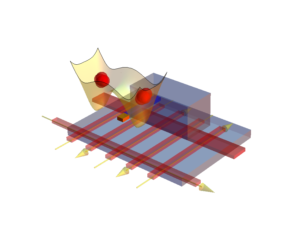
Figure 1: (Color online) Graphical representation of an atom chip that can be a realization of the model studied in this work. An array of wires is used to create two dimple traps that contain atoms (red). The traps are separated by tunable barriers. The yellow arrows indicate the currents used to create the traps. On top of the wire configuration that supports the traps, the cantilever (blue) is mounted with a tip (orange) that interacts with the atoms. The figure is inspired in the work Reichel et al. (2001).

We are interested in an anharmonic nanomechanical oscillator coupled to a BEC in such a way that its position influences the atomic current flowing between the wells of a double-well potential in which the BEC’s atoms are trapped. Thus we consider, in one dimension, a quartic anharmonic oscillator of mass $m$ and frequency $\omega_{0}$, described by the Hamiltonian

$$\hat{H}_{\hbox{\scriptsize{osc}}}=\frac{\hat{P}^{2}}{2m}+\frac{1}{2}m\omega_{0}^{2}\hat{X}^{2}+\frac{\beta}{4}\hat{X}^{4},$$ (1)

where $\beta$ controls anharmonicity of the potential. The oscillator is coupled to a BEC composed by non-interacting bosonic atoms trapped in a symmetric double well potential. Without tunnelling the atoms may occupy the left or right well

$$\hat{H}_{\hbox{\scriptsize{con}}}=E_{0}\,(\hat{c}^{\dagger}_{L}\hat{c}_{L}+\hat{c}^{\dagger}_{R}\hat{c}_{R}),$$ (2)

where the operator $\hat{c}^{\dagger}_{L}(\hat{c}^{\dagger}_{R})$ creates a boson in the ground state of the left (right) well. We choose the coupling to be linear in the the BEC’s tunnelling operator $\hat{T}=\hat{c}^{\dagger}_{L}\hat{c}_{R}+\hat{c}^{\dagger}_{R}\hat{c}_{L}$, and assuming oscillation to be small, linearise it also in the oscillator’s position $X$

$$\hat{H}_{int}=\hbar\Omega(\hat{X})\otimes\hat{T}\approx\hbar[\Omega_{0}+\Omega_{1}\hat{X}]\,(\hat{c}^{\dagger}_{L}\hat{c}_{R}+\hat{c}^{\dagger}_{R}\hat{c}_{L}).$$ (3)

Now with tunnelling switched on, the full Hamiltonian is given by Sokolovski and Gurvitz (2009)

$$\hat{H}=\hat{H}_{\hbox{\scriptsize{osc}}}+\hat{H}_{\hbox{\scriptsize{con}}}+\hat{H}_{int}.$$ (4)

Initially the system is prepared in a product state, and its density matrix has the form

$$\hat{\rho}(0)=\hat{\rho}_{\hbox{\scriptsize{osc}}}(0)\otimes\hat{\rho}_{\hbox{\scriptsize{con}}}(0),$$ (5)

where $\hat{\rho}_{\hbox{\scriptsize{con}}}(0)$ corresponds to some non-equilibrium state of the BEC. The flow of bosons across the barrier dividing the wells depends on $\hat{X}$, and may be used to extract information about the oscillator’s position. The back action provided by such a measurement on the observed oscillator is the subject of this paper. A sketch of a possible experimental setup is shown in Fig.1.

Since the trap is symmetric, the tunnelling operator commutes with the $\hat{H}_{\hbox{\scriptsize{con}}}$, $[\hat{H}_{\hbox{\scriptsize{con}}},\hat{T}]=0$. Suppose the BEC is prepared in a stationary state $|\tilde{\phi}_{n}\rangle$,

$$|\tilde{\phi}_{n}\rangle=[2^{N}(N-n)!n!]^{-1/2}\left(\hat{c}^{\dagger}_{L}+\hat{c}^{\dagger}_{R}\right)^{N-n}\left(\hat{c}^{\dagger}_{L}-\hat{c}^{\dagger}_{R}\right)^{n}|0\rangle_{\rm con}\qquad(n=0,1,..,N),$$ (6)

$$\hat{c}_{L}|0\rangle_{\rm con}=\hat{c}_{R}|0\rangle_{\rm con}=0,$$

for which we also have $\hat{H}_{\hbox{\scriptsize{con}}}|\tilde{\phi}_{n}\rangle=NE_{0}$, and $\hat{T}|\tilde{\phi}_{n}\rangle=(N-2n)|\tilde{\phi}_{n}\rangle$. It is readily seen that the BEC will continue in $|\tilde{\phi}_{n}\rangle$, while the oscillator would experience a constant energy shift of $\hbar\Omega_{0}(N-2n)$ and an additional force $\varphi_{n}\equiv\hbar\Omega_{1}(N-2n)$. Moreover, the density matrix of the oscillator at a time $t$, $\hat{\rho}_{\hbox{\scriptsize{osc}}}(t)={\rm Tr}_{\rm con}\{\rho(t)\}$, is given by a weighted sum of density matrices $\hat{\rho}_{\hbox{\scriptsize{osc}}}^{(n)}$ evolved from $\hat{\rho}_{\hbox{\scriptsize{osc}}}(0)$ under different forces $\varphi_{n}$

$$\hat{\rho}_{\hbox{\scriptsize{osc}}}(t)=\sum_{n}P(n)\,\hat{\rho}_{\hbox{\scriptsize{osc}}}^{(n)}(t),$$ (7)

where

$$\hat{\rho}_{\hbox{\scriptsize{osc}}}^{(n)}(t)\equiv e^{-i\hat{\mathcal{H}}_{\hbox{\scriptsize{osc}}}(\varphi_{n})t/\hbar}\hat{\rho}_{\hbox{\scriptsize{osc}}}(0)e^{i\hat{\mathcal{H}}_{\hbox{\scriptsize{osc}}}(\varphi_{n})t/\hbar}$$ (8)

$$\hat{\mathcal{H}}_{\hbox{\scriptsize{osc}}}(\varphi_{n})\equiv\hat{H}_{\hbox{\scriptsize{osc}}}+\varphi_{n}\hat{X},$$

and $P(n)$ is the probability to find the BEC in a state $|\tilde{\phi}_{n}\rangle$ at $t=0$,

$$P(n)={\rm Tr}_{\hbox{\scriptsize{con}}}\left[|\tilde{\phi}_{\it n}\rangle\langle\tilde{\phi}_{\it n}|\hat{\rho}_{\hbox{\scriptsize{con}}}(0)\right].$$ (9)

(We note that the constant energy shifts cancel, and do not contribute to the oscillators evolution).

Similarly, for the expectation value of an oscillator’s observable $\hat{O}$, we have

$$\langle\hat{O}\rangle=\sum_{n}P(n){\rm Tr}_{\rm osc}\left[\hat{\rho}_{\hbox{\scriptsize{osc}}}^{(n)}(t)\hat{O}\right]=\sum_{n}P(n){\rm Tr}_{\rm osc}\left[\hat{\rho}_{\hbox{\scriptsize{osc}}}(0)\hat{O}_{n}(t)\right],$$ (10)

with $\hat{O}_{n}(t)=e^{i\hat{\mathcal{H}}_{\hbox{\scriptsize{osc}}}(\varphi_{n})t/\hbar}\hat{O}e^{-i\hat{\mathcal{H}}_{\hbox{\scriptsize{osc}}}(\varphi_{n})t/\hbar}$.

We can consider a limit in which the number of bosons in the BEC increases, while the individual tunnelling probability is reduced, so that there is a finite atomic current between the two wells,

$$N\to\infty,\quad\Omega_{0,1}\to 0,\quad\Omega_{0,1}\sqrt{N}=\kappa_{0,1}.$$ (11)

Preparing all the atoms in the left well,

$$\hat{\rho}_{\hbox{\scriptsize{con}}}(0)=|\psi_{0}\rangle\langle\psi_{0}|,\quad|\psi_{0}\rangle\equiv(\hat{c}^{\dagger}_{L})^{N}|0\rangle_{{\rm{con}}}/\sqrt{N!},$$ (12)

we have a source of practically irreversible current, since the Rabi period after which the BEC returns to its initial state is now very large Sokolovski and Gurvitz (2009). Measuring after a time $t$ the number of atoms in the right well gives information about the oscillator’s past Sokolovski (2009). Also the sums in Eqs.(7) and (10) can be replaced by integrals, $\sum_{n}P(n)\to\int d\varphi P(\varphi)$. Continuous distribution of forces corresponding to the initial state (12) is Gaussian,

$$P(\varphi)=\frac{e^{-\varphi^{2}/2\Delta_{\varphi}^{2}}}{\sqrt{2\pi\Delta_{\varphi}^{2}}},$$ (13)

with $\Delta_{\varphi}^{2}\equiv 2m\hbar\omega_{0}\kappa^{2}$ Sokolovski and Gurvitz (2009).

III Monitoring position of a quartic anharmonic oscillator

The process of decoherence appears in general in the dynamics of averages of particular observables. Then, instead of analysing the density matrix (7), it is convenient to consider the oscillator’s mean position, thus choosing the operator $\hat{O}$ in Eq.(10) as the operator $\hat{X}$,

$$\langle\hat{X}(t)\rangle=\sum_{n}P(n)\langle\hat{X}_{n}(t)\rangle,$$

which reads, in the continuous limit,

$$\langle\hat{X}(t)\rangle=\int_{-\infty}^{\infty}d\varphi\,P(\varphi)\left<\hat{X}_{\varphi}(t)\right>$$ (14)

$$= \int_{-\infty}^{\infty}d\varphi\,P(\varphi)\left\{\sum_{i}\left<\psi^{\varphi}_{i}|\hat{\rho}_{\hbox{\scriptsize{osc}}}(0)|\psi^{\varphi}_{i}\right>\left<\psi^{\varphi}_{i}|\hat{X}|\psi^{\varphi}_{i}\right>+\sum_{i\neq j}e^{-i\left(E^{\varphi}_{i}-E^{\varphi}_{j}\right)t/\hbar}\left<\psi^{\varphi}_{i}|\hat{\rho}_{\hbox{\scriptsize{osc}}}(0)|\psi^{\varphi}_{j}\right>\left<\psi^{\varphi}_{j}|\hat{X}|\psi^{\varphi}_{i}\right>\right\},$$

with $\hat{\mathcal{H}}_{\hbox{\scriptsize{osc}}}(\varphi)|\psi^{\varphi}_{i}\rangle=E^{\varphi}_{i}|\psi^{\varphi}_{i}\rangle$. Indeed, it can be observed that in the case $E^{\varphi}_{i}-E_{j}^{\varphi}\neq const(\varphi)$, the exponentials in the second term of Eq.(14) are rapidly-oscillating functions and consequently such term will vanish. Therefore $\hat{\rho}_{\hbox{\scriptsize{osc}}}(t)$ [and with it the averages (10)] will tend to stationary values as $t\rightarrow\infty$. Without such a cancellation, the oscillator will not be able to reach a steady state no matter how long one waits.

Equation (14) is the starting point of the quantum calculations we shall present.

III.1 Time evolution in Wigner space

We shall first look at the time evolution of a state of the oscillator in Wigner representation when it is influenced by the condensate. In that representation, the state develops structure as time progresses. An initial state of the oscillator evolves according to a Schrödinger equation that takes into account the effect of the condensate. In one dimension the Wigner function associated to a quantum state $\hat{\rho}$ is defined as Wigner (1932)

$$W(x,p,t)=\frac{1}{2\pi\hbar}\int dq\,e^{ipq/\hbar}\Big{\langle}x-\frac{q}{2}\,\Big{|}\,\hat{\rho}\,\Big{|}\,x+\frac{q}{2}\Big{\rangle}.$$ (15)

It is convenient to write a state $\hat{\rho}$ of the oscillator for a given time $t$ in terms of the eigenstates $|\varphi_{n}\rangle$ of the harmonic oscillator as

$$\hat{\rho}(t)=\sum_{n,m}c_{nm}(t)|\varphi_{n}\rangle\langle\varphi_{m}|.$$ (16)

By inserting this expression in (15) it follows the Wigner function corresponding to the state of the oscillator as

$$W(x,p,t)=\sum_{n,m}c_{nm}(t)w_{nm}(x,p),$$ (17)

where

$$w_{nm}(x,p)=\frac{1}{2\pi\hbar}\int\,e^{ipq/\hbar}\Big{\langle}x-\frac{q}{2}\,\Big{|}\,\varphi_{n}\Big{\rangle}\Big{\langle}\varphi_{m}\Big{|}\,x+\frac{q}{2}\Big{\rangle}.$$ (18)

The integral in this expression has a representation in terms of generalized Laguerre polynomials $L_{n}^{a}$ yielding

$$w_{nm}(x,p)=\begin{cases}\frac{(-1)^{n}e^{-|z|^{2}}}{\pi\hbar}\Big{(}\frac{n!\,2^{m}}{m!\,2^{n}}\Big{)}^{1/2}(z^{*})^{m-n}L_{n}^{m-n}(2|z|^{2}),&\mbox{if}(n\leq m)\\ \\ \frac{(-1)^{m}e^{-|z|^{2}}}{\pi\hbar}\Big{(}\frac{m!\,2^{n}}{n!\,2^{m}}\Big{)}^{1/2}(z)^{n-m}L_{m}^{n-m}(2|z|^{2})&\mbox{if}(n\geq m),\end{cases}$$ (19)

with $z=x\sqrt{m\omega_{0}/\hbar}+ip\sqrt{\hbar m\omega_{0}}$. When equation (19) is combined with equation (17) it follows an analytical expression for the Wigner function of the oscillator. In Figure 2 it is plotted the Wigner function of the oscillator at different times. It can be seen that as time proceeds an initial coherent state starts to spread over phase space developing a highly oscillatory structure, that at the end is responsible for the decay of the position expectation value. It is precisely the study of such decay and of its details the subject of this work.

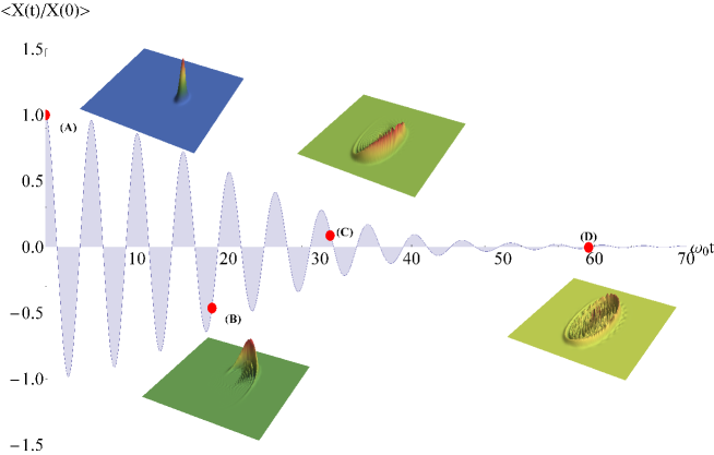
Figure 2: (Color online) Decay of the expectation value of position and some Wigner functions of the oscillator at different times.

III.2 Quasi classical approximation

We begin by evaluating the quasi classical limit of (14) which is conveniently obtained by employing the Weyl-Wigner representation Weyl (1927); Wigner (1932). For the average of an arbitrary operator describing the oscillator, $\hat{O}_{n}(t)$, we write

$$\langle\hat{O}_{n}(t)\rangle=\int_{-\infty}^{\infty}dx\,\int_{-\infty}^{\infty}dp\,W(x,p)\,O_{n}(x,p,t),$$ (20)

where $W(x,p)$ and $O_{n}(q,p,t)$ are the Weyl-Wigner transforms of the initial oscillator’s state, and of the operator $\hat{O}_{n}(t)$ in its Heisenberg representation,

$$O_{n}(x,p,t)=\int dq\,e^{ipq/\hbar}\Big{\langle}x-\frac{q}{2}\,\Big{|}\,\hat{O}_{n}(t)\,\Big{|}\,x+\frac{q}{2}\Big{\rangle}.$$ (21)

The dynamical aspects of the formalism are contained in the equation of motion for $O_{n}(x,p,t)$

$$\partial_{t}O_{n}(x,p,t)=\{\{\mathcal{H}(x,p;\varphi_{n}),O_{n}(x,p,t)\}\},$$ (22)

where $\mathcal{H}(x,p;\varphi_{n})$ is the Wigner representation of the quantum Hamiltonian operator $\hat{\mathcal{H}}_{\hbox{\scriptsize{osc}}}$, and the Moyal (Sine) bracket is defined, as usual Moyal (1949), by

$$\{\{f(x,p),g(x,p)\}\}\equiv\frac{2}{\hbar}f(x,p)\sin[\frac{\hbar}{2}(\stackrel{{\scriptstyle\leftarrow}}{{\partial_{p}}}\stackrel{{\scriptstyle\rightarrow}}{{\partial_{x}}}-\stackrel{{\scriptstyle\leftarrow}}{{\partial_{x}}}\stackrel{{\scriptstyle\rightarrow}}{{\partial_{p}}})]g(x,p)$$

with, e.g., $f(x,p)\stackrel{{\scriptstyle\leftarrow}}{{\partial_{p}}}\stackrel{{\scriptstyle\rightarrow}}{{\partial_{x}}}g(x,p)\equiv\partial_{p}f(x,p)\partial_{x}g(x,p)$. Equations (20) - (22) are a convenient starting point for our quasi classical analysis. Expanding $O_{n}(x,p,t)=X_{n}(x,p,t)$ in powers of $\hbar$, as

$$X_{n}(x,p,t)=X^{cl}_{n}(x,p,t)+\hbar^{2}X^{(2)}_{n}(x,p,t)+{\cal{O}}(\hbar^{4}),$$ (23)

and recalling that as $\hbar\to 0$ the Moyal bracket reduces to the classical Poisson bracket $\left\{*,*\right\}$ Gaspard et al. (1995), we obtain an approximate equation of motion for $X^{cl}_{n}(x,p,t)$,

$$\partial_{t}X^{cl}_{n}(x,p,t)=\Big{\{}\mathcal{H}(x,p;\varphi_{n}),X^{cl}_{n}(x,p,t)\Big{\}},$$ (24)

with the initial condition

$$X^{cl}_{n}(x,p,t=0)=x,$$ (25)

which is obtained by evaluating the integral (21) for $t=0$. A solution of the classical equation of motion (24) is any function $\mathcal{F}(x_{t}(x,p),p_{t}(x,p))$, provided $x_{t}$ and $p_{t}$ satisfy the Hamiltonian equations of motion (a dot denotes the time derivative)

$$\dot{p}_{t} =-\partial_{x_{t}}\mathcal{H}(x_{t},p_{t};\varphi_{n})= -m\omega^{2}_{0}x_{t}-\beta x^{3}_{t}-\varphi_{n}$$

$$\dot{x}_{t} =\partial_{p_{t}}\mathcal{H}(x_{t},p_{t};\varphi_{n})= p_{t}/m,$$ (26)

subject to $x_{t=0}=x$ and $p_{t=0}=p$. With the help of the initial condition (25) we identify $\mathcal{F}(x,p)$ with $x$, so that $X^{cl}_{n}(x,p,t)=x_{t}(x,p)$. Thus, $X^{cl}_{n}(x,p,t)$ is just the position, at a time $t$, of the oscillator whose initial position and momentum at $t=0$ were $x$ and $p$, respectively,

It is readily seen that in the quasi classical limit, the task of calculating the mean oscillator’s position at time $t$,

$$\langle\hat{X}(t)\rangle_{qcl}=\sum_{n}P(n)\left[\int_{-\infty}^{\infty}dx\,\int_{-\infty}^{\infty}dp\,W(x,p)\,X^{cl}_{n}(x,p,t)\right],$$ (27)

reduces to choosing initial phase space distribution $W(x,p)$, which contains all quantum effects, and evaluating classical oscillator trajectories for different values of the induced force $\varphi_{n}$. In the limit of small anharmonicity ($\frac{\beta x_{0}^{2}}{\omega_{0}^{2}}\ll 1$) the system will be shown to behave as a set of harmonic oscillators each one with a slightly shifted frequency and the semiclassical approximation described by the previous equation is very accurate for the purpose of studying the decoherence effect induced by the coupling with the BEC system. To support the accuracy of the approximations made comparisons with the results obtained by exact numerical integration of the Schrödinger equation are provided. The numerics give strong support to the semiclassical approximation in the limit we are considering.

III.3 A coherent initial state. Small anharmonicity

Next we specify our analysis to the case where the oscillator is prepared in a coherent state, whose Weyl-Wigner transform is given by

$$W(x,p)=\frac{1}{\pi\hbar}e^{-\frac{m\omega_{0}}{\hbar}(x-x_{0})^{2}-\frac{1}{m\hbar\omega_{0}}(p-p_{0})^{2}}.$$ (28)

There are no analytical solutions for a classical anharmonic oscillator. However, the decoherence effects absent for a harmonic oscillator, appear already in the limit of small anharmonicity ($\frac{\beta x_{0}^{2}}{\omega_{0}^{2}}\ll 1$). In this case approximate oscillator trajectories can be obtained, e.g., by the method of strained coordinates (Lindsted-Poincaré method) for periodic solutions Kevorkian and Cole (1981), which we will describe here briefly. We begin by considering a trajectory such that at some $t=t_{0}$ it passes through some $x^{0}$ with a zero momentum, $x_{t_{0}}=x^{0}$, $p_{t_{0}}=0$. This can be represented by a sum of harmonic functions with phases and amplitudes modified at different orders in $\beta$. An approximate solution to the first order in $\beta$ for the phase and to zero order for the amplitude is given by Kevorkian and Cole (1981); Marinca and Herisanu (2012)

$$X^{cl}_{n}({x}^{0},0,t)=-\frac{\varphi_{n}}{m\omega^{2}_{0}}+\left(\frac{\varphi_{n}}{m\omega^{2}_{0}}+{x}^{0}\right)\cos\left\{\omega_{0}\left[1+\beta\Delta({x}^{0},0;\varphi_{n})\right](t-t_{0})\right\},$$ (29)

with

$$\Delta(x,p;\varphi_{n})=\frac{3}{4(m\omega_{0}^{2})^{2}}\,{\cal{H}}_{0}(x,p;\varphi_{n})+\frac{15}{8m^{3}\omega_{0}^{6}}\,\varphi_{n}^{2}+{\cal{O}(\beta)},\qquad\qquad\qquad\qquad$$ (30)

and

$${\cal{H}}_{0}(x,p;\varphi_{n})=\frac{p^{2}}{2m}+\frac{1}{2}m\omega_{0}^{2}x^{2}+\varphi_{n}x.\qquad\qquad\qquad\qquad\qquad\qquad\qquad\qquad$$ (31)

The solution corresponding to an arbitrary choice of initial $x$ and $p$ is then obtained by choosing in Eq.(29) ${x}^{0}$ and $t_{0}$ in such a way that the trajectory specified by Eq.(29) would, at $t=0$, pass through $x$ with the desired momentum $p$. Explicitly, we have

$$X_{n}^{cl}(x,p,t)=-\frac{\varphi_{n}}{m\omega^{2}_{0}}+\left(\frac{\varphi_{n}}{m\omega^{2}_{0}}+x\right)\cos(\omega_{1}t)+\frac{p}{m\omega_{0}}\sin(\omega_{1}t),$$ (32)

which describes a harmonic motion whose frequency is modified both by the anharmonicity of the oscillator potential and the presence of the BEC, and also depends on the initial position $x$ and momentum $p$ of the oscilllator,

$$\omega_{1}=\omega_{0}\left[1+\beta\Delta(x,p;\varphi_{n})\right].$$

Higher order corrections in $\beta$ can be systematically obtained if necessary, although decoherence for small enough $\beta$ ($\frac{\beta x_{0}^{2}}{\omega_{0}^{2}}\ll 1$) is accurately described at this level of approximation. In particular a third harmonic contribution, with an amplitude which is first order in $\beta$, is negligible as compared to the decoherence/dephasing effect we will show next to be produced by the combined effect of frequency shift in the first harmonic (which is also first order in $\beta$) and the interaction with the BEC, which implies a superposition of signals with frequencies $\omega_{1}=\omega_{0}\left[1+\beta\Delta(x,p;\varphi_{n})\right]$ that contain terms $\beta\varphi_{n}$ and $\beta\varphi_{n}^{2}$, which is at the end the origin of the decoherence effect we illustrate in this work (see the details in the Appendix).

Replacing in Eq.(27) the summation over discrete levels of the BEC by integration as described in Sect. II (and changing the discrete subscript $n$ to a continuos index $\varphi$) yields

$$\langle\hat{X}(t)\rangle_{qcl}=\frac{1}{\sqrt{2\pi\Delta_{\varphi}^{2}}}\int_{-\infty}^{\infty}\int_{-\infty}^{\infty}\int_{-\infty}^{\infty}d\varphi\,dx\,dp\,\exp(-\varphi^{2}/2\Delta_{\varphi}^{2})\,W(x,p)\,X^{cl}_{\varphi}(x,p,t).$$ (33)

The integral in Eq.(33), with $W(x,p)$ and $X^{cl}_{\varphi}(x,p,t)$ given by Eqs.(28) and (32) respectively, can be evaluated analytically, e.g., by formally introducing a Gaussian generating function ${\cal Z}({\bf J})$,

$${\cal Z}({\bf J}) = e^{-C}\int\frac{d{\bf z}}{\pi\hbar\sqrt{2\pi\Delta_{\varphi}^{2}}}e^{-\frac{1}{2}{\bf z}^{T}\cdot{\mathsf{A}}\cdot{\bf z}+({\mathbf{B}}+{\bf J})^{T}\cdot{\bf z}}$$

$$= \frac{2e^{-C}}{\hbar\Delta_{\varphi}\sqrt{{\hbox{det}}{\mathsf{A}}}}\,e^{\frac{1}{2}({{\mathbf{B}}+\bf J})^{T}\cdot{\mathsf{A}}^{-1}\cdot({{\mathbf{B}}+\bf J})},$$

with ${\bf z}=(x,p,\varphi)$, ${\bf J}=(J_{1},J_{2},J_{3})$,

$${\mathsf{A}}=\left(\begin{array}[]{lll}\frac{2m\omega_{0}}{\hbar}-\frac{3it\beta}{4m\omega_{0}}&0&-\frac{3it\beta}{4m^{2}\omega_{0}^{3}}\\ 0&\frac{2}{m\hbar\omega_{0}}-\frac{3it\beta}{4m^{3}\omega_{0}^{3}}&0\\ -\frac{3it\beta}{4m^{2}\omega_{0}^{3}}&0&\frac{1}{\Delta_{\varphi}^{2}}-\frac{15it\beta}{4m^{3}\omega_{0}^{5}}\end{array}\right),\qquad\qquad\quad$$

$${\mathbf{B}}=\left(\begin{array}[]{l}\frac{2m\omega_{0}x_{0}}{\hbar}\\ \frac{2p_{0}}{m\omega_{0}\hbar}\\ 0\end{array}\right),\,{\hbox{and}}\quad C=-i\omega_{0}t+\frac{2}{\hbar\omega_{0}}\left(\frac{p_{0}^{2}}{2m}+\frac{1}{2}m\omega_{0}^{2}x_{0}^{2}\right).$$ (35)

Then defining $\overline{z_{i}}(t)\equiv\frac{\partial{\cal{Z}}}{\partial J_{i}}|_{{\bf J}=0}$, $i=1,2,3$, we have

$$\langle\hat{X}(t)\rangle_{qcl}=\frac{{\rm Re}\left[\overline{\varphi}(t)\right]}{m\omega_{0}^{2}}+{\rm Re}\left[\overline{x}(t)\right]+\frac{{\rm Im}\left[\overline{p}(t)\right]}{m\omega_{0}},$$ (36)

from which an explicit analytical expression can be derived, although we will not cite it here.

Equations (33)-(36) are the main result of this Section. In Fig. 3 we compare the analytical results in Eq. (36) with those obtained for $\langle\hat{X}(t)\rangle$ in equation (14) by numerical diagonalisation of each $\hat{\cal{H}}_{\hbox{\scriptsize{osc}}}(\varphi_{n})$. At $t=0$, the oscillator is prepared in a coherent state with $x_{0}=3\;\hbox{a.u.}$, and $p_{0}=0$, $\beta$ has been set to $0.05\;\hbox{a.u.}$ and $\omega_{0}=1.3\;\hbox{a.u.}$ which justifies the perturbative approach of Eqs.(29)-(32). The agreement between both results is good, and we proceed to use the quasi classical Eq.(36) in order to characterise the decoherence in the short and the long time limits.

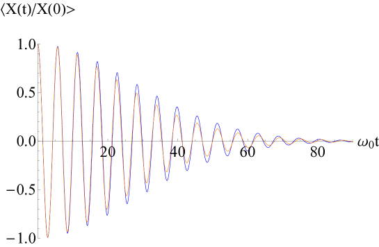
Figure 3: (Color online) Comparison between the quasiclassical solution (36) (orange line) and the exact numerical solution of the equations of motion (blue line) in the perturbative regime ($\beta x_{0}^{2}/2m\omega_{0}^{2}=0.133$) for an initial coherent state with $x_{0}=3$, $p_{0}=0$, $\omega_{0}=1.3$, $\beta=0.05$ and $\Delta_{\varphi}=0.1$ (atomic units are used).

III.4 Time scale analysis

If the oscillator is not coupled to the condensate then it will show a coherent motion in which coherences will remain in time leading to recurrences in the oscillator dynamics. The action of the condensate quenches such recurrences. We shall assume that the coupling between the condensate and the oscillator is such that recurrences in the dynamics of the oscillator have been suppressed and therefore the decoherence process occurs in a time scale much shorter than the dynamical recurrence time of the free (uncoupled) oscillator.

There are two relevant processes with regard to the time development and decay of $\langle\hat{X}(t)\rangle_{qcl}$: The non-linearity in the potential, and the interaction with the condensate. As already emphasized, when such non-linearity does not exists the coupling between the oscillator and the condensate will not lead to a decay in oscillator’s expectation values, even if variances and higher order fluctuations are affected by such coupling Brouard et al. (2011). However, the non-linear potential together with the oscillator-condensate interaction induces decoherence. A natural time scale linked to such non-linearity can be defined as $t_{\beta}=(3\beta\hbar/4m^{2}\omega_{0}^{2})^{-1}$. In addition, the interaction between the oscillator and the condensate introduces a different time scale, given by $t_{\varphi}=(3\beta\Delta_{\varphi}^{2}/4m^{3}\omega_{0}^{5})^{-1}$. Both time scales are different and they are useful to understand the time development of oscillator’s observables. We shall analyze the dynamics in two different situations, for $t$ either smaller or larger than both characteristic time scales.

III.4.1 Case 1: $t\ll t_{\beta},t_{\varphi}$

In this case the solution is accurately represented by

$$\langle\hat{X}(t)\rangle_{qcl}\simeq e^{-t^{2}/2t^{2}_{G}}\left[x_{0}\cos(\omega_{1}t)+\frac{p_{0}}{m\omega_{0}}\sin(\omega_{1}t)\right],$$ (37)

with $\omega_{1}=\omega_{0}+\frac{3\beta\hbar}{4m^{2}\omega_{0}^{2}}\frac{{\cal{H}}(x_{0},p_{0};0)}{\hbar\omega_{0}}=\omega_{0}+\Delta\omega_{0}$, and

$$t_{G}=t_{\beta}\left(\frac{\hbar\omega_{0}}{{\cal{H}}(x_{0},p_{0};0)+m\omega_{0}^{2}x_{0}^{2}t_{\beta}/t_{\varphi}}\right)^{1/2}.$$ (38)

It is apparent that $t_{G}$ is a natural time scale associated with a Gaussian decoherence process taking place for times smaller than $t_{\beta}$ and $t_{\varphi}$. Furthermore, a fully Gaussian decay, including a Gaussian tail, will develop if $t_{G}\ll t_{\beta}$, $t_{\varphi}$. That situation will appear in a fully semiclassical regime. In the quantum domain $t_{G}$ will be of the order of or smaller than $t_{\varphi}$ leading to a decay which will not be Gaussian. In the limit of harmonic potential a coherent motion as reported in Brouard et al. (2011) is recovered, emphasizing the relevance of the non-linearity to the decoherence process.

III.4.2 Case 2: $t\gg t_{\beta},t_{\varphi}$

In this case the solution can be represented by using a long time approximation by

$$\langle\hat{X}(t)\rangle_{qc}\simeq e^{{-2\frac{{\cal{H}}(x_{0},p_{0};0)}{\hbar\omega_{0}}}}\frac{m^{11/2}\omega_{0}^{13/2}}{\hbar^{2}\Delta\varphi}\frac{64}{9\sqrt{3}}(\beta t)^{-5/2}\left(x_{0}\cos\omega_{0}t+\frac{p_{0}}{m\omega_{0}}\sin\omega_{0}t\right)+{\cal{O}}\left({(\beta t)}^{-7/2}\right).$$ (39)

The agreement of this expression with the numerical exact solutions to the quantum equations has been checked for small $\beta$ ($\frac{\beta x_{0}^{2}}{\omega_{0}^{2}}\ll 1$). We observe that if time is much larger than $t_{\beta}$ and $t_{\varphi}$ the decay is algebraic. Notably the amplitude is exponentially damped as $\exp(-{\cal{H}}(x_{0},p_{0};0)/\hbar\omega_{0})$, therefore this suggests that deeply within the quasiclassical regime, in consistency with the results of the previous section, it would be difficult to observe such power law decay, indicating that such dynamics would be observable mainly within the quantum domain.

The decay of observables shows an initial Gaussian decay for short times and a power law decay for longer times. Our results are consistent with those in Braun et al. (2001); Strunz et al. (2003); Žnidarič and Prosen (2005) where Gaussian decoherence was studied.

In the next section we present numerical simulations as well as some analytical approximate expressions describing the dynamics of the system in the full quantum regime.

III.5 Quantum Analysis

For the quantum case and an arbitrary value of $\beta$ there are no analytical solutions. Numerical solutions can be obtained efficiently by diagonalizing $\hat{H}_{\hbox{\scriptsize{osc}}}+\varphi\hat{X}$ over a truncated basis of stationary states of the harmonic oscillator centered at the origin, for each value of $\varphi$. Convergence with respect to the number of basis states used for the truncated diagonalization is checked for each particular value of $\beta$ and for the initial state of the oscillator. These numerical results are used all throughout the paper to compare with the different analytical approximations described.

In the general case, for arbitrary values of $\beta$, many different time-dependent terms will contribute to the sum in (14). However, in some limiting cases and under some approximations, analytical expressions can be obtained that describe the time decay with accuracy.

We will consider here as an illustration the case of an initial state of the oscillator involving only a few lower-energy states of the oscillator with frequency $\omega_{0}$ and a value of $\hbar\beta\ll m^{2}\omega_{0}^{3}$.

Let us focus on the time-dependent part of Eq.(14),

$$\langle\hat{X}(t)\rangle-\langle\hat{X}\rangle^{st}=\frac{1}{\sqrt{2\pi\Delta_{\varphi}^{2}}}\int_{-\infty}^{\infty}d\varphi\,e^{-\varphi^{2}/2\Delta_{\varphi}^{2}}\sum_{i<j}e^{-i\left(E^{\varphi}_{i}-E^{\varphi}_{j}\right)t/\hbar}F_{i,j}(\varphi)+c.c.,$$ (40)

where the superscript “st” stands for stationary and with $F_{i,j}(\varphi)\equiv\left<\psi^{\varphi}_{i}|\hat{\rho}_{\hbox{\scriptsize{osc}}}(0)|\psi^{\varphi}_{j}\right>\left<\psi^{\varphi}_{j}|\hat{X}|\psi^{\varphi}_{i}\right>$.

Firstly, for not too large values of $\Delta_{\varphi}$, it is enough to write the energy eigenvalues as a second order expansion in $\varphi$, $E^{\varphi}_{i}(\beta)=E^{\varphi=0}_{i}(\beta)+\gamma_{i}\varphi^{2}$, (the term linear in $\varphi$ is zero because the anharmonicity is even in the $x-$coordinate). A first order approximation in $\beta$ for $E^{\varphi=0}_{i}(\beta)$ and $\gamma_{i}$,

$$E^{\varphi=0}_{i}=\hbar\omega_{0}\left(i+\frac{1}{2}\right)+\frac{3\hbar^{2}\beta\,\left(i^{2}+i+\frac{1}{2}\right)}{8m^{2}\omega_{0}^{2}},$$ (41)

$$\gamma_{i}=-\frac{1}{2m\omega_{0}^{2}}+\frac{3\hbar\beta\left(2i+1\right)}{4m^{3}\omega_{0}^{5}},$$ (42)

will be sufficient for the states that will contribute to the summation.

A valid approximation for $F_{i,j}(\varphi)$ can be obtained to zeroth order in $\beta$. Writting the initial state of the oscillator in terms of the stationary states of the harmonic oscillator, $\left|\psi_{n}\right>$, as $\hat{\rho}_{\hbox{\scriptsize{osc}}}(0)=|\psi(0)\rangle\langle\psi(0)|$, with $|\psi(0)\rangle=\sum_{n}c_{n}|\psi_{n}\rangle$, and evaluating $\left<\psi^{\varphi}_{i}|\psi_{n}\right>$ and $\left<\psi^{\varphi}_{j}|\hat{X}|\psi^{\varphi}_{i}\right>$ as integrals over $x$, one obtains

$$\left<x|\psi_{n}^{\varphi}\right>=\sqrt{\frac{1}{2^{n}\,n!}}\left(\frac{m\omega_{0}}{\pi\hbar}\right)^{1/4}\,H_{n}(y)e^{-y^{2}/2},$$ (43)

with $y=\sqrt{\frac{m\omega_{0}}{\hbar}}\left(x-\frac{\varphi}{m\omega_{0}^{2}}\right)$, for the displaced $n$th stationary state of the harmonic oscillator. Thus finally $F_{i,j}(\varphi)$ reads

$$F_{i,j}(\varphi)=G_{i,j}(\varphi)e^{-\varphi^{2}/(2m\hbar\omega_{0}^{3})},$$ (44)

where $G_{i,j}(\varphi)=g_{i,j}^{(0)}+g_{i,j}^{(2)}\varphi^{2}$ is a known polynomial of $\varphi$. The odd powers will not contribute to the integral. Furthermore, only terms up to the second order will be kept.

For an initial state being a combination of the first two lower-energy states of the harmonic oscillator, $|\psi(0)\rangle=c_{0}|\psi_{0}\rangle+c_{1}|\psi_{1}\rangle$, the mean value of position then reads,

$$\langle\hat{X}(t)\rangle=\langle\hat{X}\rangle^{st} + \sum_{n=0,1}\frac{e^{-i\omega_{n,n+1}t}}{\sqrt{2\Delta_{\varphi}^{2}}}\left(g_{n,n+1}^{(0)}\sqrt{\frac{1}{1/(2\Delta_{\varphi}^{2})+1/(2m\hbar\omega_{0}^{3})+i(\gamma_{n}-\gamma_{n+1})t}}\right.$$ (45)

$$+ \left.\frac{1}{2}g_{n,n+1}^{(2)}\left(\frac{1}{1/(2\Delta_{\varphi}^{2})+1/(2m\hbar\omega_{0}^{3})+i(\gamma_{n}-\gamma_{n+1})t}\right)^{3/2}\right)+{\rm c.c},$$

where $\omega_{n,n+1}\equiv E_{n}^{\varphi=0}-E_{n+1}^{\varphi=0}$. Fig. 4 shows exact numerical results compared to the analytical approximation given by Eq. (45). The inset presents the two curves for large time, where the analytical approximation is shown to reproduce both the frequency and the amplitude of the oscillations with great accuracy. The coefficients $g_{n,n+1}^{(0)}$ and $g_{n,n+1}^{(2)}$ depend on the coefficients in the Hermite polynomials, $H_{n}(x)$, as well as on $c_{0}$ and $c_{1}$ characterizing the state $|\psi(0)\rangle$,

$$g_{0,1}^{(0)}=\left(\frac{\hbar}{2m\omega_{0}}\right)^{1/2}\,c_{0}c_{1}^{*}$$

$$g_{0,1}^{(2)}=-\left(\frac{2m\omega_{0}}{\hbar}\right)^{1/2}\,\frac{c_{0}^{*}c_{1}+c_{0}c_{1}^{*}}{4m^{2}\omega_{0}^{4}}$$

$$g_{1,2}^{(0)}=0$$

$$g_{1,2}^{(2)}=\left(\frac{2m\omega_{0}}{\hbar}\right)^{1/2}\,\frac{c_{0}^{*}c_{1}+2c_{0}c_{1}^{*}}{4m^{2}\omega_{0}^{4}}.$$

If only the term $n=0$ is considered, a first order approximation in $\beta$ is used for the difference $\gamma_{0}-\gamma_{1}=-3\hbar\beta/(2m^{3}\omega_{0}^{5})$, and $G_{0,1}(\varphi)$ is taken as $g_{0,1}^{(0)}$. A good qualitative approximation is already obtained for this case,

$$\langle\hat{X}(t)\rangle\simeq\langle\hat{X}\rangle^{st}+g_{0,1}^{(0)}\,e^{-i\omega_{0,1}t}\sqrt{\frac{1}{1+2\Delta_{\varphi}^{2}/(2m\hbar\omega_{0}^{3})+3i\Delta_{\varphi}^{2}\frac{\hbar\beta}{m^{3}\omega_{0}^{5}}t}}+c.c.$$ (46)

The envelope of $\langle\hat{X}(t)\rangle$ in Eq. (46) is also shown for comparison in Fig 4.

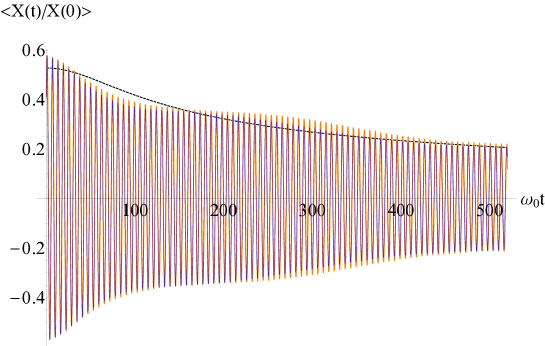
Figure 4: (Color online) Mean value of position as a function of $\omega_{0}t$ (normalized to its initial value) for an initial state of the oscillator $|\psi(0)\rangle=\left(1+i\right)|\psi_{0}\rangle/\sqrt{3}+i|\psi_{1}\rangle/\sqrt{3}$. Numerical result (solid line) and the analytical approximation given by Eq. (45) (dashed line) are almost indistinguishable in the figure. Frequency and amplitude of the signal are described with great accuracy by the analytical expression. The envelope of the analytical approximation in Eq. (46) is shown for reference (dotted line). The inset shows the details of the evolution for the expectation value of position in the large time region. $\beta=0.05$, $\omega_{0}=1.3$, $\Delta_{\varphi}=0.7$ (a.u.)

Power law decay for the amplitude of the oscillations is observed, the different powers that contribute to the result depending on the initial state, being of the general form $t^{-k/2}$, with $k$ being an integer.

IV Conclusions

A detailed study of decoherence of an anharmonic oscillator in contact with a BEC trapped in a double well potential is performed. The oscillator is coupled to the BEC through its position. In contrast with the harmonic oscillator case, for which coherent behaviour has been reported, the anharmonic oscillator presents anomalous decoherence (non-exponential). In the quasiclassical domain there are two clearly distinguishable regimes. For short times, decoherence appears to be Gaussian with a well defined time scale. Such time scale depends on the degree of anharmonicity of the oscillator as well as on the energy distribution of the initial state of the whole system. The higher the anharmonicity of the oscillator and/or the energy distribution of the initial state, the faster is the decay of coherence in short time scales. All that in consistency with a quantum-to-classical transition. On the other hand, at long times coherence decays algebraically. The particular power of the decay is characteristic of the initial states considered. The observation of both time regimes requires a very fine tuning of the initial state of the system, in particular of its initial energy distribution as measured by the energy variance. In the full quantum domain decoherence manifests itself in a combination of pure algebraic decay processes for all times of the form $t^{-k/2}$ ($k$ an integer) according to the decomposition of the initial state of the oscillator in the harmonic oscillator number basis. This would allow to observe coherent motion for longer times that what it would be possible with an exponential decay. Our results show that a slight anharmonicity in the confining potential of the oscillator is sufficient to observe anomalous decoherence.

*

Appendix A Third harmonic contribution

It is known that the contribution of higher harmonics to the dynamics of the anharmonic oscillator may be relevant Marinca and Herisanu (2012). In fact, one can explicitly compute the solution $x(t)$ of $\ddot{x}=-\omega_{0}^{2}x-\beta x^{3}$ with $x(0)=x_{0}$ and $\dot{x}(0)=0$, which includes those higher harmonics i.e.

$$x(t) =x_{0}\cos\omega t+\frac{\beta x_{0}^{3}}{32\omega^{2}}\left(\cos 3\omega t-\cos\omega t\right)+\frac{\beta^{2}x_{0}^{5}}{1024\omega^{4}}\left(\cos 5\omega t-\cos\omega t\right)+...,$$ (47)

$$\hbox{with}\quad\omega^{2} =\frac{1}{16}\left[6\beta x_{0}^{2}+8\omega_{0}^{2}+\sqrt{30\beta^{2}x_{0}^{4}+96\beta x_{0}^{2}\omega_{0}^{2}+64\omega_{0}^{4}}\right].$$

Such solution is rather accurate even for a non moderate anharmonic contribution. However, in this work we restrict ourselves to the analysis of small anharmonicity for which $\frac{\beta x_{0}^{2}}{\omega_{0}^{2}}\ll 1$ and hence $\omega\approx\omega_{0}+\frac{3\beta x_{0}^{2}}{8\omega_{0}}$. In such limit the phases are slightly corrected and the amplitudes of higher harmonics are negligible with respect to the first harmonic amplitude because $\frac{\beta x_{0}^{2}}{\omega_{0}^{2}}\ll 1$ implies $\frac{\beta x_{0}^{2}}{\omega^{2}}\ll 1$ and $\frac{\beta^{2}x_{0}^{4}}{\omega^{4}}\ll 1$. So, in the limit we are considering, the main contribution to $x(t)$ comes from the first harmonic. Let us remark that as soon as the anharmonicity starts to be important higher harmonics should be considered but this is out of our aim in the present work.

At this stage a second aspect becomes relevant. The whole quantum signal (or its semiclassical approximation) is a superposition of individual $x(t;x_{0},p_{0},\varphi)$ that are averaged over initial conditions $x_{0},p_{0}$ and over the parameter $\varphi$ that measures the action of the condensate on the oscillator, see equations (29)-(31). The phase correction depends on the initial condition and $\varphi$. Therefore, when averaging, the net result of such superposition will be a dephased signal, that eventually decays. It happens that the decay will be shown to be fast enough so that along the decay time, $x(t;x_{0},p_{0},\varphi)$, described by its first harmonic approximation, will be in fact an accurate description of the oscillators dynamics. The conclusion is that to characterize the decay in the parameter domain we are studying ($\frac{\beta x_{0}^{2}}{\omega_{0}^{2}}\ll 1$), it is enough to take into account the first correction in the phase and the first harmonic approximation.

References

- Hunger et al. (2010) D. Hunger, S. Camerer, T. W. Hänsch, D. König, J. P. Kotthaus, J. Reichel, and P. Treutlein, Phys. Rev. Lett. 104, 143002 (2010).
- Treutlein et al. (2012) P. Treutlein, C. Genes, K. Hammerer, M. Poggio, and P. Rabl, (2012), 1210.4151 .
- Reichel et al. (2001) J. Reichel, W. Hänsel, P. Hommelhoff, and T. Hänsch, Applied Physics B: Lasers and Optics 72, 81 (2001).
- Schwab and Roukes (2005) K. C. Schwab and M. L. Roukes, Physics Today 58, 36 (2005).
- Kippenberg and Vahala (2008) T. J. Kippenberg and K. J. Vahala, Science 321, 1172 (2008), http://www.sciencemag.org/content/321/5893/1172.full.pdf .
- Treutlein et al. (2007) P. Treutlein, D. Hunger, S. Camerer, T. W. Hänsch, and J. Reichel, Phys. Rev. Lett. 99, 140403 (2007).
- Meiser and Meystre (2006) D. Meiser and P. Meystre, Phys. Rev. A 73, 033417 (2006).
- Genes et al. (2008) C. Genes, D. Vitali, and P. Tombesi, Phys. Rev. A 77, 050307 (2008).
- Ian et al. (2008) H. Ian, Z. R. Gong, Y.-x. Liu, C. P. Sun, and F. Nori, Phys. Rev. A 78, 013824 (2008).
- Camerer et al. (2011) S. Camerer, M. Korppi, A. Jöckel, D. Hunger, T. W. Hänsch, and P. Treutlein, Phys. Rev. Lett. 107, 223001 (2011).
- Vogell et al. (2013) B. Vogell, K. Stannigel, P. Zoller, K. Hammerer, M. T. Rakher, M. Korppi, A. Jöckel, and P. Treutlein, Phys. Rev. A 87, 023816 (2013).
- Hammerer et al. (2009) K. Hammerer, M. Aspelmeyer, E. S. Polzik, and P. Zoller, Phys. Rev. Lett. 102, 020501 (2009).
- Hensinger et al. (2005) W. K. Hensinger, D. W. Utami, H.-S. Goan, K. Schwab, C. Monroe, and G. J. Milburn, Phys. Rev. A 72, 041405 (2005).
- Singh et al. (2008) S. Singh, M. Bhattacharya, O. Dutta, and P. Meystre, Phys. Rev. Lett. 101, 263603 (2008).
- O’Connell et al. (2010) A. D. O’Connell, M. Hofheinz, M. Ansmann, R. C. Bialczak, M. Lenander, E. Lucero, M. Neeley, D. Sank, H. Wang, M. Weides, J. Wenner, J. M. Martinis, and A. N. Cleland, Nature 464, 697 (2010).
- Blencowe et al. (2005) M. P. Blencowe, J. Imbers, and A. D. Armour, New Journal of Physics 7, 236 (2005).
- Gurvitz and Mozyrsky (2008) S. A. Gurvitz and D. Mozyrsky, Phys. Rev. B 77, 075325 (2008).
- Mozyrsky and Martin (2002) D. Mozyrsky and I. Martin, Phys. Rev. Lett. 89, 018301 (2002).
- Regal et al. (2008) C. A. Regal, J. D. Teufel, and K. W. Lehnert, Nature Physics 4,, 555 (2008), 0801.1827 .
- Armour and Blencowe (2008) A. D. Armour and M. P. Blencowe, New Journal of Physics 10, 095004 (25pp) (2008).
- Blencowe and Armour (2008) M. P. Blencowe and A. D. Armour, New Journal of Physics 10, 095005 (23pp) (2008).
- Zurek (1991) W. H. Zurek, Physics Today 44, 36 (1991).
- Brouard et al. (2011) S. Brouard, D. Alonso, and D. Sokolovski, Phys. Rev. A 84, 012114 (2011).
- Sokolovski and Gurvitz (2009) D. Sokolovski and S. A. Gurvitz, Phys. Rev. A 79, 032106 (2009).
- Sokolovski (2009) D. Sokolovski, Phys. Rev. Lett. 102, 230405 (2009).
- Wigner (1932) E. Wigner, Phys. Rev. 40, 749 (1932).
- Weyl (1927) H. Weyl, Z. Phys 46, 1 (1927).
- Moyal (1949) J. E. Moyal, Mathematical Proceedings of the Cambridge Philosophical Society 45, 99 (1949).
- Gaspard et al. (1995) P. Gaspard, D. Alonso, and I. Burghardt, Advances in Chemical Physics 90, 105 (1995).
- Kevorkian and Cole (1981) J. Kevorkian and J. Cole, Perturbation methods in applied mathematics (Springer-Verlag New York, 1981).
- Marinca and Herisanu (2012) V. Marinca and N. Herisanu, Nonlinear Dynamical Systems in Engineering: Some Approximate Approaches (Springer, 2012).
- Braun et al. (2001) D. Braun, F. Haake, and W. T. Strunz, Phys. Rev. Lett. 86, 2913 (2001).
- Strunz et al. (2003) W. T. Strunz, F. Haake, and D. Braun, Phys. Rev. A 67, 022101 (2003), 115.
- Žnidarič and Prosen (2005) M. Žnidarič and T. Prosen, Journal of Optics B: Quantum and Semiclassical Optics 7, 306 (2005).