Optical Multi-Channel Intensity Interferometry – or:
How To Resolve O-Stars in the Magellanic Clouds

1 Introduction

Non est ad astra mollis e terris via.
There is no easy way from the Earth to the stars.

— Seneca the Younger (c. 54), Hercules Furens

The demand for ever higher angular resolution in astronomy has driven the development of interferometric techniques since the mid of the 19th century (e.g., Fizeau 1868; Stéphan 1874; Michelson 1891). Almost all astronomical interferometers ever constructed are amplitude interferometers, based on the coherent superposition of electromagnetic waves. A second, less well known, approach is provided by intensity interferometry, based on correlations of fluctuations in the intensities of radiation: the Hanbury Brown–Twiss effect.

The history of Hanbury Brown–Twiss intensity interferometry (HBTII) may well be regarded as a “perfect science story”:

$\bullet$ from the discovery of a phenomenon: correlated intensity fluctuations in the light received from an astronomical source of radiation (Hanbury Brown, Jennison & Das Gupta, 1952; Hanbury Brown & Twiss, 1954);

$\bullet$ to the development of the corresponding theory: photon-photon correlation in coherent beams of radiation (Hanbury Brown & Twiss, 1957a);

$\bullet$ to the experimental validation of the theory (Hanbury Brown & Twiss, 1957b; Twiss & Little, 1959);

$\bullet$ and, eventually, toward an astronomical application: optical stellar interferometry (Hanbury Brown & Twiss, 1958a, b).

The discoveries of the 1950s evolved into the construction of a dedicated observatory, the Narrabri Stellar Intensity Interferometer (NSII) in Narrabri, Australia (Hanbury Brown et al., 1964; Hanbury Brown, Davis & Allen, 1967). The instrument was composed of two movable 6.7-meter diameter light collectors, spanning a maximum baseline of $b=188$ meters length. As the instrument worked at a wavelength $\lambda=440$ nm, its best angular resolution was $\theta\approx 1.2\lambda/b\approx 0.6$ milliseconds of arc (mas). This resolving power was used for measuring directly the angular diameters of a sample of 32 bright stars (Hanbury Brown et al., 1967; Hanbury Brown, 1968; Hanbury Brown, Davis & Allen, 1974) – the NSII was the first astronomical instrument ever able to do so. However, despite the large collecting areas of $\approx$30 m² for each light collector, photon statistics limited the NSII to targets with apparent $B$ band magnitudes $m_{B}<2.5$. Accordingly, the instrument was shut down in 1972, after having completed its survey of stellar diameters. A successor was proposed around this time but not built eventually; this decision was based on the – incorrect – assumption that amplitude interferometry would be available for astronomy soon. A detailed review of intensity interferometry and the NSII is provided by Hanbury Brown (1974). Today, stellar intensity interferometry is standard content of optics textbooks (cf., e.g., Fowles 1975; Goodman 1985; Mandel & Wolf 1995; Born & Wolf 1999; Loudon 2000; Kitchin 2009)

In this article, we review and discuss the theory, concepts, and limitations of optical intensity interferometry. Building upon recent technical developments we argue that the sensitivity of an NSII-type interferometer can be improved by a factor of approximately 100, corresponding to 5 photometric magnitudes. This is possible by using (i) avalanche photodiodes (APD) as light detectors, and (ii) distributing the light received from the source over multiple spectral channels. When deploying interferometer arrays with multiple large light collectors equivalent to modern long-baseline radio interferometers, it is possible to achieve limiting $R$-band magnitudes up to $m_{R}\approx 14$, corresponding to an improvement in sensitivity by a factor $\approx$25 000 relative to the Narrabri interferometer. Such multi-channel intensity interferometers would provide new opportunities for observational astronomy in a variety of science cases ranging from stellar physics to the physics of supermassive black holes.

2 Amplitude Interferometry

2.1 Interference and Coherence

The concept of amplitude interferometry is based on the superposition of electromagnetic waves. (The following discussion is based on: Born & Wolf 1999; Loudon 2000; Labeyrie, Lipson & Nisenson 2006; Glindemann 2011.) If this superposition is coherent, the waves interfere; the interference pattern can be analyzed to obtain the properties of the source of radiation. The degree of coherence of two electric field waves $E$ observed at times $t_{i}$ and positions ${{\bf x}}_{i}$ (located in a plane perpendicular to the direction of light propagation), with $i=1,2$, is quantified by the complex first-order coherence function

$$\gamma({{\bf x}}_{1},t_{1},{{\bf x}}_{2},t_{2})=\frac{{\langle}E^{*}({{\bf x}}_{1},t_{1})E({{\bf x}}_{2},t_{2}){\rangle}}{\sqrt{{\langle}|E({{\bf x}}_{1},t_{1})|^{2}{\rangle}{\langle}|E({{\bf x}}_{2},t_{2})|^{2}{\rangle}}}$$ (1)

where ^∗ marks a complex conjugate, and $|...|$ and ${\langle}...{\rangle}$ denote the absolute value and the time average of the enclosed expressions, respectively. By construction, $|\gamma|\in[0,1]$, where a value of 1 denotes coherent light, a value of 0 denotes incoherent light, and intermediate values denote partial coherence. Being a complex function, $\gamma$ can be expressed as $\gamma=|\gamma|\exp(i\phi)$, with $\phi$ denoting the phase. As $\gamma$ is a function of time and position, coherence is referred to as temporal coherence or spatial coherence depending on context. For convenience, $\gamma$ is usually expressed as function of differential positions and times, i.e., $\gamma({{\bf x}}_{1},t_{1},{{\bf x}}_{2},t_{2})\rightarrow\gamma({{\bf d}},\tau)$, with ${{\bf d}}={{\bf x}}_{1}-{{\bf x}}_{2}$ and $\tau=t_{1}-t_{2}$.

The necessity of temporal coherence demands that the time delay $\tau$ between two light beams has to be much smaller than their coherence time $\tau_{c}$ – i.e., $\tau\ll\tau_{c}$ – to warrant $|\gamma|\approx 1$. For $\tau\gg\tau_{c}$, $|\gamma|=0$, and interference is not possible. For light with an optical bandwidth $\Delta\nu$, with $\nu$ being the frequency of radiation, the coherence time is given by

$$\tau_{c}\approx\frac{1}{\Delta\nu}~{}.$$ (2)

The coherence time can be expressed in terms of the coherence length $w_{c}=c\tau_{c}$, with $c$ denoting the speed of light. Evidently, any path difference $w$ between the light beams has to fulfill $w\ll w_{c}$ in order to preserve coherence.

The conditions for spatial coherence are expressed by the van Cittert–Zernicke theorem. The theorem states that the intensity distribution of an incoherent, quasi-monochromatic source and the coherence function are a Fourier transform pair. For a two-dimensional astronomical source with angular coordinates $\theta_{1},\theta_{2}$ and sky intensity distribution $I(\theta_{1},\theta_{2})$, this may be written like

$$\gamma({{\bf d}})\stackrel{{\scriptstyle\mathcal{F}}}{{\rightleftharpoons}}I(\theta_{1},\theta_{2})$$ (3)

where $\mathcal{F}$ denotes a Fourier transform. Accordingly, the image of a source can be derived by measuring the complex coherence function and applying a Fourier transform to it. An example important in astronomy is the case of a circular source with angular diameter $\theta$, for which

$$|\gamma(d)|=\left|\frac{2J_{1}(\zeta)}{\zeta}\right|$$ (4)

where $J_{1}$ is the Bessel function of first order and first kind, $\zeta=\pi d\theta/\lambda$, and $d=|{{\bf d}}|$. This $|\gamma(d)|$ reaches zero value for the first time at $\zeta=3.83$, corresponding to $\theta=1.22\,\lambda/d$, leading to the well-known resolution criterion of Rayleigh. The distribution of intensity, $|\gamma(d)|^{2}$, then corresponds to the well-known Airy intensity profile.

The general coherence function $\gamma({{\bf d}},\tau)$ is conveniently expressed as function of the $uv$ coordinates ${\bf u}=(u,v,w)$. Any astronomical interferometer is an array of two or more telescopes. For each pair of telescopes, their spatial separation is given by a physical baseline vector ${\bf b}=(b_{x},b_{y},b_{z})$ which is defined relative to the local Earth tangential plane. By convention, $b_{x}$ is the telescope distance in north-south direction, $b_{y}$ is the distance in east-west direction, and $b_{z}$ is the distance in vertical direction, i.e., a height difference. By construction, $d\leq b$ with $b=|{\bf b}|$. The vector u, in units of observation wavelength $\lambda$, is derived by projection of ${\bf b}$ onto the plane of the sky at the position of the target. For the projection formula, see, e.g., Ségransan (2007).

For one given time and wavelength, each pair of telescopes provides a measurement of $\gamma$ in the plane spanned by $u$ and $v$, $\gamma(u,v)$. The van Cittert–Zernicke theorem relates $\gamma(u,v)$ and $I(\theta_{1},\theta_{2})$ like

$$\gamma(u,v)\stackrel{{\scriptstyle\mathcal{F}}}{{\rightleftharpoons}}I(\theta_{1},\theta_{2})~{}.$$ (5)

Accordingly, we may define a uv radius $\rho$ via $\rho^{2}=u^{2}+v^{2}=(d/\lambda)^{2}$. In this notation, the angular resolution of a baseline is then $\theta\approx 1/\rho$. The coordinate $w$ corresponds to the path difference, and thus the delay, between the light rays arriving at the two telescopes. This delay needs to be controlled carefully to ensure $w\ll w_{c}$. By symmetry (because the selection of the origin of ${\bf b}$ is arbitrary), each measurement actually provides two values, $\gamma(u,v)$ and $\gamma(-u,-v)=\gamma^{*}(u,v)$.

2.2 Radio Astronomy

Radio interferometry (Thompson, Moran & Swenson, 2004; Wilson, Rohlfs & Hüttemeister, 2010) is based on preserving the full wave (amplitude and phase) information of the infalling radiation while recording it. This is achieved by heterodyne receivers that shift the signal frequency to lower values by mixing the astronomical signal with a stable reference wave provided by a local oscillator. The output electric voltage can be transmitted and processed almost arbitrarily by use of dedicated electronics. Especially, it is straightforward to correlate the signals from different antennas and to calculate $\gamma({\bf u})$ according to Equation (1).

The technical simplicity of radio interferometry made it a standard technique in observational astronomy. Traditionally, radio interferometers are classified according to their physical extensions: long-baseline interferometry (LBI) denotes interferometry with arrays composed of several, physically separate telescopes. Signals from different antennas are usually correlated and processed in real time. Very long baseline interferometry (VLBI) refers to arrays that are too extended – potentially extending across the entire Earth – to combine the signals from individual telescopes in real time. In VLBI arrays, the signal of any antenna is stored locally by powerful (magnetic tape or hard disk) recorders, together with an accurate time reference signal usually provided by an atomic clock. The amplitudes from individual antennas are then correlated off-line.

2.3 Optical Astronomy

At wavelengths shorter than a few micrometers, fundamental quantum noise limits prevent the use of heterodyne receiving techniques. In order to achieve interference, the light from two (or more) apertures has to be combined directly by superposition (Labeyrie, Lipson & Nisenson, 2006; Glindemann, 2011). Physical information is obtained by recording and analysis of the resulting interference pattern. The fringe contrast, or visibility, obeys $V\propto|\gamma({\bf u})|$. The missing information on the phase $\phi$ is obtained from the intensity at the center position ($\rho=0$) of the fringe pattern. This results in a complex visibility ${\mathcal{V}}\equiv V\exp(i\phi)\propto\gamma({\bf u})$.

The direct combination of light rays imposes severe constraints on the stability and mechanical tolerances of an optical interferometer. As stated by Equation (2), a wide optical bandpass leads to very short coherence times. Assuming observations at $\lambda=500$ nm through a narrow band filter with bandpass $\Delta\lambda=10$ nm, we find $\Delta\nu=1.2\times 10^{13}$ Hz. From this one finds a correlation time of $\tau_{c}\approx 10^{-13}$ s, corresponding to a correlation length $w_{c}\approx 30\,\mu$m. As interference requires $w\ll w_{c}$, we need to control the geometry of our interferometer within accuracies on the order of few micrometers. This may be compared to the case of radio interferometry with typical $\Delta\nu\approx 1$ GHz, resulting in $w_{c}\approx 0.3$ m.

A further complication arises from atmospheric turbulence. Fluctuations of the atmosphere lead to random variations of the phase of the fringe pattern on time scales of few milliseconds. For exposure times longer than this atmospheric coherence time, the fringe pattern, and thus the visibility, is averaged out. Additionally, radiation propagating through the atmosphere remains coherent only on spatial scales on the order of 10 cm. The use of telescope apertures substantially larger than the atmospheric coherence scale further weakens the interference pattern.

3 Intensity Interferometry

3.1 Intensity Correlations

Figure 1: The second-order coherence function $\gamma^{(2)}$, as function of time delay $\tau$ in units of coherence time $\tau_{c}$. The continuous curve indicates the case of chaotic light with Gaussian frequency profile. The dotted line with a constant value of unity corresponds to the behavior of monochromatic coherent light (laser, maser).

Optical intensity interferometry exploits correlated fluctuations in the intensity of the radiation received from a source. Else than for optical amplitude interferometry, the radiation arriving at any antenna (telescope) is converted into an electronic signal by a detector immediately upon reception at the antenna. Only the electronic signals – not the light rays – are transmitted to a correlator and combined; accordingly, an intensity interferometer may be regarded as a cross of optical and radio interferometers, with an optical frontend – light collectors, optics, photodetectors – and a radio backend – signal transmission, electronics, correlators. The electronic signal from each antenna carries information on the intensity $I(t)$ of the recorded light.

Intensity interferometry exploits the fact that intensities received at different antennas show correlated fluctuations. This can be understood (Hanbury Brown & Twiss, 1957a; Hanbury Brown, 1974) by regarding the electromagnetic waves emitted by a pair of point sources P_a,b with amplitudes $E_{a,b}$, angular frequencies $\omega_{a,b}$, and phases $\phi_{a,b}$ (see also Figure 2a). The intensities recorded at two antennas A_1,2 are then

$$I_{1} = \big{[}E_{a}\sin(\omega_{a}t+\phi_{a})+E_{b}\sin(\omega_{b}t+\phi_{b})\big{]}^{2}$$

$$I_{2} = \big{[}E_{a}\sin(\omega_{a}(t+\tau_{a})+\phi_{a})$$ (6)

$$+\,E_{b}\sin(\omega_{b}(t+\tau_{b})+\phi_{b})\big{]}^{2}$$

where $\tau_{a,b}$ are delays due to optical path differences between the two antennas. Each of the two expressions results in a sum of a constant direct current component plus oscillating terms that correspond to harmonics, sums, and differences of the two frequencies. By application of appropriate high-pass and low-pass filters, it is possible to suppress all terms except the one corresponding to the difference of $\omega_{a}$ and $\omega_{b}$, eventually leaving us with two beat terms

$$\Delta I_{1} = E_{a}E_{b}\cos\big{[}(\omega_{a}-\omega_{b})t+(\phi_{a}-\phi_{b})\big{]}$$

$$\Delta I_{2} = E_{a}E_{b}\cos\big{[}(\omega_{a}-\omega_{b})t+(\phi_{a}-\phi_{b})$$ (7)

$$+\,\omega_{a}\tau_{a}-\omega_{b}\tau_{b}\big{]}$$

Evidently, $\Delta I_{1}$ and $\Delta I_{2}$ are identical except of a phase term $\omega_{a}\tau_{a}-\omega_{b}\tau_{b}$. Correlating, i.e., multiplying the two intensities, and assuming $\omega_{a}\approx\omega_{b}\equiv\omega$, results in

$$\Delta I_{1}\Delta I_{2}=E_{a}^{2}E_{b}^{2}\cos\left[\omega(\tau_{a}-\tau_{b})\right]$$ (8)

or, assuming the points $P_{a,b}$ have angular distance $\theta$,

$$\Delta I_{1}\Delta I_{2}=E_{a}^{2}E_{b}^{2}\cos\left[2\pi b\theta/\lambda\right]~{}.$$ (9)

Integrating Equation (9) over all possible pairs of points P_a,b, all frequencies $\omega_{a,b}$, and all frequency differences $\omega_{a}-\omega_{b}$ for a given target source leads to the conclusion (Hanbury Brown & Twiss, 1957a) that the product $\Delta I_{1}\Delta I_{2}$ is proportional to $|\gamma|^{2}$. Accordingly, the correlation of fluctuations of intensities observed at antennas A_1,2 provides information on the source structure.

Figure 2: Basic concepts of intensity interferometry. a: Observation layout. Two antennas A_1,2 located at a distance $b$ observe a target. Each antenna observes an intensity given by a superposition of electric waves emitted by pairs of point sources P_a,b. At each antenna, the intensity is recorded and converted into an electronic signal. The signals are combined by a correlator C. Optical path differences are compensated by an electronic delay $\tau$ in one of the interferometer arms. b: Signal processing scheme. Two detectors D_1,2 located in antennas A_1,2 record voltages with intensities $I_{1,2}(t)$. Each signal is passed through a high-pass filter HP that suppresses the constant direct current component, leaving the fluctuating components $\Delta I_{1,2}(t)$. The fluctuation signals are multiplied (device $\times$) and averaged in time (device ${\langle}\cdot{\rangle}$), resulting in the averaged product ${\langle}\Delta I_{1}\Delta I_{2}{\rangle}$ at the output. Separately, the time averaged intensities ${\langle}I_{1,2}{\rangle}$ are computed and stored.

3.2 Second-Order Coherence

In analogy to Equation (1) for electromagnetic waves, the degree of correlation among intensities $I$ is quantified (Loudon, 2000; Labeyrie, Lipson & Nisenson, 2006) by the second-order coherence function

$$\gamma^{(2)}({{\bf d}},\tau)=\frac{{\langle}I({{\bf x}},t)I({{\bf x}}+{{\bf d}},t+\tau){\rangle}}{{\langle}I({{\bf x}},t){\rangle}{\langle}I({{\bf x}}+{{\bf d}},t+\tau){\rangle}}$$ (10)

where the superscript ^(m) denotes coherence of $m$-th order ($m>1$); ${{\bf d}}$ and $\tau$ are the parameters already used in Section 2.1. The temporal second-order coherence, $\gamma^{(2)}\equiv\gamma^{(2)}(\tau)$ (i.e., ${{\bf d}}=0$), is a function of the photon statistics of the radiation to be analyzed (Loudon, 2000; Bachor & Ralph, 2004). For monochromatic coherent light with Poissonian photon statistics, as provided by lasers or masers, $\gamma^{(2)}(\tau)=1$ for all $\tau$. This is distinct from the case of chaotic light, referring to radiation composed of electric waves with random amplitudes that follow a Gaussian distribution; this includes especially thermal black-body radiation. Chaotic light obeys super-Poissonian statistics, commonly referred to as photon bunching, resulting in characteristic $\gamma^{(2)}(\tau)$ profiles. In general, $\gamma^{(2)}(0)=2$ and $\gamma^{(2)}(\tau\gg\tau_{c})=1$, with $\tau_{c}$ being the coherence time according to Equation (2). The exact shape of the $\gamma^{(2)}(\tau)$ curve depends on the frequency profile of the light (see, e.g., Chapter 3.7 of Loudon 2000 for details). In Figure 1, we show the $\gamma^{(2)}(\tau)$ profile of chaotic light with Gaussian frequency profile (Gaussian–Gaussian light) alongside the trivial case of coherent light.

For the case of chaotic light, a generalization of the analysis introduced in Section 3.1 finds a general relation between the first-order coherence function $\gamma({{\bf d}},\tau)$ and the second-order coherence function $\gamma^{(2)}({{\bf d}},\tau)$ given by

$$\gamma^{(2)}({{\bf d}},\tau)=1+|\gamma({{\bf d}},\tau)|^{2}$$ (11)

(Loudon, 2000; Labeyrie, Lipson & Nisenson, 2006). Accordingly, an analysis of the second-order coherence function provides the squared modulus of the first-order coherence function. Notably, this statement holds for both, temporal and spatial coherence. This means that an intensity interferometer provides information on the spatial structure of the target source similar to an amplitude interferometer. The most important difference is the loss of phase information as only the modulus of $\gamma$ is preserved. As a consequence, it is not possible to reconstruct the complete source image by Fourier transformation of the $uv$ plane data, as this requires the complex function $\gamma(\bf u)$.

In general, each pair of antennas A_1,2 of an astronomical intensity interferometer records intensities $I_{1,2}(t)$. By subtraction of the time averages of the intensities ${\langle}I(t){\rangle}$, we obtain the intensity fluctuations around the averages, $\Delta I_{1,2}(t)=I_{1,2}(t)-{\langle}I_{1,2}(t){\rangle}$. Here time averages are taken over periods much longer than the resolving time $\tau_{d}$ of the light detectors, and shorter than the time scales of any variability of the source brightness. By comparison of Equation (10) and Equation (11), one finds the convenient relation

$$|\gamma({{\bf d}},\tau)|^{2}=\frac{{\langle}\Delta I_{1}\Delta I_{2}{\rangle}}{{\langle}I_{1}{\rangle}{\langle}I_{2}{\rangle}}$$ (12)

which provides $|\gamma({{\bf d}},\tau)|^{2}$ from correlation of the intensity fluctuations. In Figure 2b, we present the corresponding signal processing scheme of an intensity interferometer (see also, e.g., Chapter 6.3.1 of Goodman 1985). Two detectors D_1,2 record voltages with intensities $I_{1,2}$. Each intensity is averaged in time, providing ${\langle}I_{1,2}{\rangle}$ at the corresponding outputs. The intensity fluctuations $\Delta I_{1,2}$ are obtained by passing the signals through electronic high-pass filters that suppress (subtract) the direct current components ${\langle}I_{1,2}{\rangle}$. The intensity fluctuations are multiplied and the product is averaged in time, eventually providing ${\langle}\Delta I_{1}\Delta I_{2}{\rangle}$. From the various output parameters it is straightforward to compute the normalized correlation

$$c(u,v)=\frac{{\langle}\Delta I_{1}\Delta I_{2}{\rangle}}{{\langle}I_{1}{\rangle}{\langle}I_{2}{\rangle}}$$ (13)

Obviously, Equation (12) and Equation (13) are equivalent; our correlation analysis simply provides the squared modulus of the first-order coherence function as function of $uv$ plane location (the delay $w$ will be discussed in Section 3.3).

At this point, we encounter a difficulty which arises from the properties of photo detectors. As already discussed in Section 2.3, we have to deal with coherence times $\tau_{c}\lesssim 10^{-13}$ s in optical interferometry. The shortest resolving times $\tau_{d}$ are provided by photomultiplier tubes (PMT) and avalanche photodiodes (APD) which are known from various applications in astronomy (Renker, 2007; Kitchin, 2009); modern, commercially available, versions of these detectors provide $\tau_{d}\gtrsim 5\times 10^{-10}$ s. Comparison with Figure 1 shows that for $\tau\geq\tau_{d}\gg\tau_{c}$, observed correlations $c(u,v)$ will be much smaller than unity, and only slightly larger than zero, for all $u,v$. Accordingly, a more practical parameter is the normalized correlation factor

$$\Gamma(u,v)=\frac{c(u,v)}{c(0,0)}$$ (14)

which expresses the correlation $c(u,v)$ in units of the correlation obtained at the origin of the $uv$ plane.

As $\Gamma(u,v)\propto|\gamma(u,v)|^{2}$ by construction, the normalized correlation factor encodes the spatial source structure on a convenient scale. Accordingly, the relation between $\Gamma(u,v)$ and the spatial intensity distribution of an astronomical source are given by the van Cittert–Zernicke theorem, however with the limitation that phase information is not preserved. The source structure is found by fitting an appropriate parametric model to the $\Gamma(u,v)$ data, with the model being the normalized square modulus of the Fourier transform of the theoretical source structure (Hanbury Brown & Twiss, 1958a, b). The arguably most important example is the measurement of stellar diameters with the NSII (Hanbury Brown, 1974): when approximating a star as a uniform circular disk, the corresponding model for $\Gamma$ is an Airy profile as obtained by taking the square of Equation (4); the angular diameter of the stellar disk is then derived from measurements of $\Gamma(\rho)$, with $\rho=d/\lambda$ being the $uv$ radius. The first zero point of the Airy profile – marking the point where a source is resolved entirely, according to the Rayleigh criterion – corresponds to an angular disk diameter of $\theta=1.22\lambda/d$; for example: at $\lambda=700$ nm, a star with angular diameter $\theta=1$ mas is resolved entirely by a projected baseline of $d=176$ m. For the Narrabri interferometer, $\lambda=440$ nm, $d=188$ m at most, and accordingly the resolution limit was $\theta=0.59$ mas (Hanbury Brown, Davis & Allen, 1967). We present the profile of $\Gamma(\rho)$ for the case of a uniform circular disk source in Figure 3. In Figure 4 we show examples for the $\Gamma(u,v)$ distributions of (a) a disk-like, circular star; (b) a rotation-flattened, elliptical star; (c) a close binary system; and (d) a close triple star system, respectively.

Figure 3: Correlation factor $\Gamma$ as function of $\zeta=\pi\theta\rho=\pi\theta d/\lambda$, if the target source is a uniform circular disk. The first zero point, where the source is resolved entirely, is located at $\zeta=3.83$, corresponding to $\theta=1.22\lambda/d$. For example: at $\lambda=700$ nm, a star with angular diameter $\theta=1$ mas is resolved entirely by a projected baseline of $d=176$ m.

The phase information, which is lost by correlating the intensities recorded at two antennas, may be retrieved by means of a triple correlation (Gamo, 1963; Sato et al., 1978). This approach makes use of third-order coherence which relates the signals from three antennas like

$$\Gamma^{(3)}\equiv\frac{{\langle}\Delta I_{1}\Delta I_{2}\Delta I_{3}{\rangle}}{{\langle}I_{1}{\rangle}{\langle}I_{2}{\rangle}{\langle}I_{3}{\rangle}}~{}.$$ (15)

For a given triple of antennas $(1,2,3)$, the parameter $\Gamma^{(3)}$ is related to the first-order coherence function $\gamma$ like

$$\Gamma^{(3)}=a|\gamma_{12}||\gamma_{13}||\gamma_{23}|\cos(\psi)$$ (16)

where $a$ is a constant, $\gamma_{ij}$ is the first-order coherence function derived for the antenna pair $ij$, and $\psi$ is given by

$$\psi=\phi_{12}-\phi_{13}+\phi_{23}$$ (17)

where $\phi_{ij}\equiv-\phi_{ji}$ denotes the phase of $\gamma_{ij}$. The relations given in Equations (16) and (17) are equivalent to the closure phase relations known from amplitude interferometry (Jennison, 1958). For an array of $M$ antennas, the number of unknown phases equals the number of baselines $N_{\Join}=M(M-1)/2$, whereas the number of independent triangles of antennas, and thus values of $\Gamma^{(3)}$, is $N_{\bigtriangleup}=(M-1)(M-2)/2$. As $N_{\Join}-N_{\bigtriangleup}=M-1$, the number of unknowns always exceeds the number of closure phases; a reliable determination of the $\phi_{ij}$ requires either large $M$ or the presence of $M-3$ redundant baselines (Labeyrie, Lipson & Nisenson, 2006). As noted by Holmes & Belen’kii (2004); Nuñez et al. (2012a, b), the phase information can also be recovered by application of the Cauchy–Riemann equations to the $uv$ data, sufficient sampling of the $uv$ plane provided.

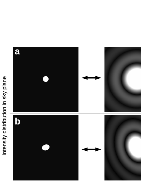
Figure 4: Sky plane vs. uv plane intensity distributions for various target source geometries. All scales are arbitrary. a: A disk-like circular star; the profile shown in Figure 3 corresponds to a 2-dimensional cut through the $uv$ plane distribution shown here. b: An elliptical, rotation-flattened star, with axis ratio $4:3$. c: A binary system of two disk-like circular stars of equal brightness and size, separated by 3.2 times the stellar diameter. d: A triple star system with relative brightnesses (stars from bottom to top) $3:2:1$.

3.3 Coherence Times and Tolerances

The coherence time, and thus the coherence length, relevant for intensity interferometers derive from the properties of the photodetectors and the signal processing system. The maximum frequency of an excitation that can be recorded by photodetectors is found from the Nyquist theorem:

$$f_{\rm max}=\frac{1}{2\tau_{d}}$$ (18)

with $\tau_{d}$ denoting the time resolution of the detector. From comparison to Equation (7) it is evident that $f_{\rm max}$ corresponds to the highest beat frequency $(\omega_{a}-\omega_{b})$ observable by a detector. For a realistic signal processing system (see Section 3.1 and Figure 2b), only signals with frequencies above a certain minimum frequency $f_{\rm min}$ will be processed by the system; frequencies lower than $f_{\rm min}\lesssim 1$ MHz will be suppressed by high-pass filters. Eventually, we obtain the electronic bandwidth

$$\Delta f=f_{\rm max}-f_{\rm min}$$ (19)

which is simply the difference of maximum and minimum signal frequencies. For practical instruments, $f_{\rm max}\gg f_{\rm min}$, and, accordingly, $\Delta f\approx f_{\rm max}$.

The electronic bandwidth $\Delta f$, rather than the optical bandwidth $\Delta\nu$, defines the coherence time of an intensity interferometer

$$\tau^{\prime}_{c}\approx\frac{1}{\Delta f}$$ (20)

and, accordingly, the coherence length $w^{\prime}_{c}=c\tau^{\prime}_{c}$. This expression may be compared to Equation (2). As noted in Section 3.2, realistic photodetectors have $\tau_{d}\gtrsim 5\times 10^{-10}$ s, meaning $\Delta f\approx f_{max}\lesssim 1$ GHz. Accordingly, $\tau^{\prime}_{c}\gtrsim 10^{-9}$ s and $w^{\prime}_{c}\gtrsim 0.3$ m; evidently, optical intensity interferometers are highly insensitive to deviations from a perfect array geometry. Mechanical tolerances of several centimeters are very easy to meet technically; notably, the tolerances derived here for optical intensity interferometers are very similar to the tolerances of radio amplitude interferometers (see Sections 2.2 and 2.3) – which represent a technology well-known since the 1950s. This may be compared to the tolerances of optical amplitude interferometers which are on the order of micrometers (see Section 2.3). Likewise, optical path differences $w$ occurring during an observation need to be controlled down to levels of few centimeters (and not micrometers); this is achieved by introducing an electronic delay into one arm of the interferometer that compensates the time delay $\tau$. A comparison with Equation (8) shows that the treatment of delays does not influence the results obtained, as for any realistic astronomical observation $\tau\approx\tau_{a}\approx\tau_{b}$ and $\tau_{a}-\tau_{b}\ll\tau^{\prime}_{c}$.

The implementation of a minimum frequency $f_{\min}$ by means of electronic high-pass filters is usually the technically easiest method to separate $\Delta I$ from ${\langle}I{\rangle}$, as illustrated in Figure 2b; a reasonable (though somewhat arbitrary) value is $f_{\min}\approx 1$ MHz. Using those values introduces an additional major advantage of optical intensity interferometers over optical amplitude interferometers. Optical amplitude interferometers are severely limited by atmospheric fluctuations (see also Section 2.3) that occur on frequency scales $\lesssim$1 kHz. Accordingly, any $f_{\min}\gg 1$ kHz filters out atmospheric fluctuations of phases and amplitudes – meaning that optical intensity interferometers are insensitive to atmospheric turbulence (Hanbury Brown, 1974; Labeyrie, Lipson & Nisenson, 2006).

3.4 Signal-to-Noise Limits

3.4.1 Statistical Limit

Intensity interferometry is based on the correlation of signals obtained by photoelectric detection of light. Accordingly, we may conduct a semi-classical statistical analysis of the photoelectron counts (Goodman, 1985; Loudon, 2000; Labeyrie, Lipson & Nisenson, 2006). Assuming the generation of $n$ photoelectrons within one detector resolution time $\tau_{d}\gg\tau_{c}$, one obtains the variance of the photoelectron count

$$\sigma_{n}^{2}=n\left[1+n\left(\frac{\tau_{c}}{\tau_{d}}\right)\right]$$ (21)

where $\tau_{c}$ is the coherence time of the light. The first summand, of order $n$, corresponds to Poisson noise. The second summand, of order $n^{2}$, represents super-Poissonian or wave noise, corresponding to macroscopic fluctuations of the light intensity; these intensity fluctuations form the signal of an intensity interferometer. Accordingly, a signal-to-noise ratio ($S/N$) of unity corresponds to the case where both summands are equal, meaning

$$n\left(\frac{\tau_{c}}{\tau_{d}}\right)=1~{}.$$ (22)

To obtain a statistical $S/N$ for an arbitrary observing time $t$, Poisson statistics tells us that we need to scale Equation (22) by a factor $\sqrt{t/\tau_{d}}$, resulting in

$$\left(\frac{S}{N}\right)_{\rm s}=n\left(\frac{1}{\tau_{d}\,\Delta\nu}\right)\left(\frac{t}{\tau_{d}}\right)^{1/2}$$ (23)

where we used $\tau_{c}=1/\Delta\nu$ (Equation (2)). The number of photoelectrons, $n$, collected by a telescope within the time $\tau_{d}$ can be expressed as

$$n=\alpha\,A\,n_{\nu}\,\Delta\nu\,\eta\,\tau_{d}$$ (24)

where $\alpha\in[0,1]$ is the quantum efficiency of the photodetectors, $A$ is the collecting area of the light collector, $n_{\nu}$ is the number of photons per time, per unit area, and per unit bandwidth, $\Delta\nu$ is the bandwidth, and $\eta\in[0,1]$ is the efficiency of the instrument (except detector quantum efficiency). Using also $\tau_{d}=1/(2\Delta f)$ (for $f_{\rm min}\ll f_{\rm max}$; Equations (18) and (19)), we obtain

$$\left(\frac{S}{N}\right)_{\rm s}=\alpha\,A\,n_{\nu}\,\eta\,\left(2\,t\,\Delta f\right)^{1/2}~{}.$$ (25)

At this point, we have to consider two additional effects. Firstly, we need to multiply Equation (25) with the normalized correlation factor $\Gamma(u,v)$ to take into account spatial coherence. Secondly, Equation (25) is strictly correct only for fully polarized light; for unpolarized light – as usual in astronomy – the observed correlation signal is reduced by a factor of two because orthogonal polarizations are uncorrelated (Hanbury Brown, 1974; Goodman, 1985). Eventually, we obtain the signal-to-noise ratio of an intensity interferometer:

$$\left(\frac{S}{N}\right)_{\rm s}=\alpha\,A\,n_{\nu}\,\eta\,\Gamma(u,v)\,\left(\frac{t\,\Delta f}{2}\right)^{1/2}~{}.$$ (26)

Scaling Equation (26) to practical values, one obtains the intuitive expression

$$\left(\frac{S}{N}\right)_{\rm s} = 46\left(\frac{\alpha}{0.2}\right)\left(\frac{A}{30\,{\rm m}^{2}}\right)\left(\frac{\eta}{0.2}\right)$$

$$\times \left(\frac{n_{\nu}}{9\times 10^{-5}\,{\rm m}^{-2}\,{\rm s}^{-1}\,{\rm Hz}^{-1}}\right)$$

$$\times \left(\frac{t}{1\,{\rm h}}\right)^{1/2}\left(\frac{\Delta f}{100\,{\rm MHz}}\right)^{1/2}\Gamma(u,v)~{}.$$

The reference values for $\alpha$, $A$, $\eta$, and $\Delta f$ correspond to values typical for the Narrabri intensity interferometer (Hanbury Brown, 1974). A photon flux of $n_{\nu}=9\times 10^{-5}\,{\rm m}^{-2}\,{\rm s}^{-1}\,{\rm Hz}^{-1}$ corresponds to the photon flux from a star observed at $\lambda\approx 500-800$ nm ($V,R,I$ bands) with an apparent photometric magnitude of zero (Bessell, 1979), attenuated by $\approx$10% due to atmospheric extinction (e.g., Lim et al. 2009). Assuming that realistic observations require $S/N\gtrsim 5$ for $\Gamma(u,v)=1$ and observing times $t=1$ h, we may conclude that the limiting photometric magnitude for an intensity interferometer with the technical parameters of the NSII is $m_{X}\approx 2.5$, $X=V,R,I$.

3.4.2 Photon Degeneracy Limit

An additional sensitivity constraint is imposed by the properties of the source of radiation. The maximum signal-to-noise ratio is limited by the number of correlated photons actually emitted by the target. Accordingly, it is possible to derive (Goodman 1985, their Chapter 9.5) the photon degeneracy limited signal-to-noise ratio

$$\left(\frac{S}{N}\right)_{\rm p}=\alpha\,\eta\,\Gamma(u,v)\,\left(\frac{t\,\Delta f}{2}\right)^{1/2}\,\chi$$ (28)

where $\chi$ is the degeneracy parameter, i.e., the average number of photons occurring in a single coherence interval of the incident radiation. For the well-known case of blackbody radiation, Bose-Einstein statistics leads to

$$\chi=\left[\exp\left(\frac{h\nu}{kT}\right)-1\right]^{-1}$$ (29)

where $h$ is Planck’s constant, $k$ is Boltzmann’s constant, and $T$ is the thermodynamic temperature of the emitter. Provided that the optical bandpass $\Delta\nu$ is sufficiently small, Equation (29) can also be applied to non-thermal radiation with an effective temperature. The effective temperature is defined as the temperature of blackbody radiation with the same intensity, at the given wavelength, as the non-thermal radiation (Gamo, 1966).

Table 1: Photon degeneracy limited source temperatures

Filter	$\lambda$ [nm]	$T^{\rm a}$ [K]	$T^{\rm b}$ [K]
$U$	360	5380	3420
$B$	440	4400	2800
$V$	550	3520	2240
$R$	640	3030	1930
$I$	790	2450	1560

Temperatures $T$ are the minimum source temperatures required for achieving $(S/N)_{\rm p}=10$, as function of observing wavelength $\lambda$ (Equations (28) and (29)). For each wavelength, we quote two limiting temperatures for two sets of parameters.
^a For $\Gamma(u,v)=1$, $t=1$ h, $\alpha=0.2$, $\eta=0.2$, $\Delta f=100$ MHz.
^b For $\Gamma(u,v)=1$, $t=1$ h, $\alpha=0.8$, $\eta=0.2$, $\Delta f=32$ GHz.

From Equations (28) and (29) it is evident that $(S/N)_{\rm p}$ is a strong function of source temperature and observing wavelength. Assuming that a practical astronomical observation requires $(S/N)_{\rm p}\gtrsim 10$ at $\Gamma(u,v)=1$ within one hour of observing time, the necessary effective temperatures are on the order of several thousand Kelvin throughout the optical spectrum. In Table 1, we present the temperatures required for $(S/N)_{\rm p}=10$ for various optical wavelengths. Both sets of temperatures assume $\Gamma(u,v)=1$ and one hour of observing time, but different instrumental parameters – the first one (case a) corresponding to the NSII, the second one (case b) to an improved instrument. The resulting values provide two conclusions: firstly, even vast technical improvements ease the temperature limits by factors less than two. Secondly, optical intensity interferometry is limited to hot astronomical targets – mostly stars. With limiting temperatures $\gtrsim$2 000 K, all stellar spectral types, as well as all stellar luminosity classes, are observable (Drilling & Landolt, 2000).

3.5 Applications

The overview provided in the previous sections leaves us with an ambivalent picture of optical intensity interferometry.

On the one hand, intensity interferometry is a very simple and robust technique. As it processes electronic signals instead of combining light rays directly, intensity interferometers can, essentially, be assembled from technology well-known for radio interferometers, at compatible cost and effort. For realistic electronic bandwidths, coherence lengths are on the order of tens of centimeters; accordingly, intensity interferometers are very tolerant with respect to mechanical aberrations and uncertainties in the coordinates $u,v,$ and $w$. As a side effect, intensity interferometers do not require high-quality telescopes as light collectors but rather simple “light buckets”, meaning coarse (with tolerances on the order of centimeters) parabolic reflectors, in analogy to atmospheric Cherenkov telescope arrays which have aperture diameters of tens of meters (Hanbury Brown, 1974; Lorenz, 2004; Aharonian et al., 2006; Lacki, 2011). The insensitivity with respect to atmospheric turbulence provides an additional advantage over optical amplitude interferometry. Furthermore, optical intensity interferometers are very powerful scientific instruments: they are the only optical interferometers that can achieve baseline lengths on scales of kilometers; as intensity interferometers do not need to combine light rays directly, their baselines are not limited in length. Accordingly, the angular resolution $\theta$ of optical intensity interferometers, in practical units, can be written as

$$\frac{\theta}{\mu\rm as}=176\left(\frac{\lambda}{700\,\rm nm}\right)\left(\frac{d}{1\,\rm km}\right)^{-1}$$ (30)

when using the Rayleigh criterion (cf. Equation (4)). A hypothetical global intensity interferometer array with $d\approx 10\,000$ km could achieve angular resolutions on the order of tens of nanoseconds of arc – a sufficiently bright and spatially concentrated science target provided.

On the other hand, optical intensity interferometry is severely handicapped by its limitations in sensitivity. The photon degeneracy limit restricts the technique to hot astronomical targets, especially stars. The statistical sensitivity limit restricts intensity interferometry to bright astronomical targets. Observatories of the type of the Narrabri interferometer are limited to apparent magnitudes $\lesssim$2.5; accordingly, the NSII was eventually restricted to observations of 32 stars (Hanbury Brown, 1974).

In summary, we see that optical intensity interferometry bears the potential of being a very important and powerful astronomical technique if its statistical sensitivity (Equations (26) and (3.4.1)) can be improved substantially at acceptable cost and effort. In recent years, multiple studies have noted this possibility and have explored possible applications for modern optical intensity interferometers (LeBohec & Holder, 2006; Ofir & Ribak, 2006a, b; Klein, Guelman & Lipson, 2007; Solomos, 2008; Foellmi, 2009; Barbieri et al., 2009; Dravins, 2010; Dravins et al., 2010; LeBohec et al., 2010; Nuñez et al., 2012a, b; Dravins et al., 2012, 2013; Rou et al., 2013), including the implementation of a working group within the International Astronomical Union (Barbieri et al., 2009) and of the dedicated Star Base Utah test facility near Salt Lake City, USA (LeBohec et al., 2010). These studies largely exploit the remarkable technical similarities between optical intensity interferometers and Cherenkov air shower telescopes with respect to light collection, photo-detection, and electronic signal processing. Current and future Cherenkov telescopes (are expected to) have collecting areas on the order of several hundred to several thousand square meters (Lorenz, 2004; Aharonian et al., 2006; Nuñez et al., 2012a; Dravins et al., 2013); using these telescopes in a – secondary – intensity interferometry mode permits sensitivities higher by factors of several hundred compared to the NSII (which had collecting areas of $\approx$30 m²; see Equation (3.4.1)). In addition, the sensitivity of astronomical interferometers – regardless of type – scales with the number of baselines, $N_{\Join}$, like $(S/N)_{\rm s}\propto\sqrt{N_{\Join}}$ due to improved sampling of the $uv$ plane (cf. Section 2.1); accordingly, adding additional light collectors to an array improves the sensitivity further.

4 Multi-Channel Intensity Interferometry

Complementary to the studies mentioned in Section 3.5 which largely concentrate on collecting areas and numbers of baselines, we now focus on the factor

$$\aleph\equiv\left(\frac{\alpha}{0.2}\right)\left(\frac{\Delta f}{100\,{\rm MHz}}\right)^{1/2}$$ (31)

taken from Equation (3.4.1). The reference values for the quantum efficiency, $\alpha=0.2$, and the electronic bandwidth, $\Delta f=100$ MHz, correspond to the case of the NSII (Hanbury Brown, 1974). These values originate from the use of photomultiplier tubes and represent the state of the art of the 1970s. Modern, commercially available PMT show values up to $\alpha\approx 0.25$ and $\Delta f\approx 1$ GHz (e.g., Renker 2007), meaning $\aleph\approx 4$ – a noteworthy, albeit not substantial improvement.

Evidently, we need to apply more sophisticated methods of photo-detection in order to increase $\aleph$ substantially. Especially promising for our purpose are semiconductor, specifically silicon, avalanche photodiodes (Si-APDs – e.g., Renker 2007; Kitchin 2009). With $\alpha\approx 85$%, they outperform PMTs by factors $\approx$4 with respect to quantum efficiency. The quantum efficiency of Si-APDs is a strong function of wavelength and peaks around 700 nm; accordingly, any astronomical instrument making use of Si-APDs is sensitive mostly in $R$ band.

Even more important than the high quantum efficiency of APDs is their electronic bandwidth. Firstly, APDs provide maximum sampling rates similar to modern PMTs, meaning electronic bandwidths up to $\Delta f\approx 1$ GHz. Secondly, APDs are sufficiently small – few millimeters – to be operated in detector arrays, with each array pixel corresponding to one APD (e.g., Anderhub et al. 2011). As already noted by Hanbury Brown (1974), this can be used to increase the instrumental sensitivity by observing spectrally dispersed light from the source with multiple photodetectors simultaneously at different wavelengths – i.e., in multiple spectral channels.

The basic idea of multi-channel intensity interferometry follows from Equation (26) in a straightforward manner. The sensitivity of an intensity interferometer is proportional to the number of photons per unit bandwidth and independent of the total number of photons. We assume that the light from the source is spectrally dispersed at two light collectors before reaching the photodetectors. For simplicity, we further assume that observations are limited to a sufficiently small part of the source spectrum such that both $n_{\nu}$ and $\alpha$ may be regarded as approximately constant – usually meaning few tens of nanometers in wavelength, avoiding known spectral lines. At both light collectors “1” and “2” we divide the spectral band into $N_{\diamond}$ channels of equal width which are monitored by detectors $i=1,2,...,N_{\diamond}$; accordingly, we record intensities $I_{1,i}$ and $I_{2,i}$. We now apply the signal processing scheme outlined in Figure 2b to each of the $N_{\diamond}$ spectral channels separately. For each $i$, we compute correlation factors $\Gamma_{i}(u,v)$ according to Equation (14). Eventually, we obtain a combined correlation factor from averaging over all spectral channels, meaning $\Gamma(u,v)={\langle}\Gamma_{i}(u,v){\rangle}_{i}$. As we average over $N_{\diamond}$ independent measurements, the statistical signal-to-noise ratio of $\Gamma(u,v)$ is higher than that of any $\Gamma_{i}(u,v)$ by a factor $\sqrt{N_{\diamond}}$. Following Hanbury Brown (1974), we express this relation in terms of an effective electronic bandwidth

$$\Delta f\longrightarrow\Delta f^{\prime}\equiv N_{\diamond}\,\Delta f$$ (32)

which enters into Equations (26), (3.4.1), (28), and (31) accordingly.

Avalanche photodiodes can be combined into detector arrays similar to early charge-coupled device (CCD) detector arrays; the largest APD arrays in use comprise about 1 000 pixels (e.g., Anderhub et al. 2011, 2013). Those APD arrays can be placed inside a spectrometer and record the dispersed source light; each detector pixel along the direction of dispersion then corresponds to one spectral channel. Else than for the case of CCDs, which have electronic bandwidths of few kHz at best, each pixel of an APD array provides a bandwidth on the order of few hundred MHz up to about one GHz. Accordingly, even small APD arrays are able to improve $\Delta f^{\prime}$, and thus $\aleph$, substantially.

In order to achieve a realistic estimate of $\aleph$, we have to regard the quantum efficiency as well as the effective electronic bandwidth. For Si-APDs, maximum quantum efficiencies are $\alpha\approx 85$% (at $\lambda\approx 700$ nm); this value is set by solid-state physics and, evidently, is already close to optimum. The effective electronic bandwidth is – a priori – only limited by the size of APD arrays and the abilities of the signal processing electronics. Signal processing systems of current long baseline radio interferometers are able to handle signal bandwidths up to 32 GHz (e.g., Schuster et al. 2008; Boissier et al. 2009). In case of an optical intensity interferometer equipped with Si-APD arrays, this value may be achieved by using, e.g., 64 spectral channels of 500 MHz each. Assuming thus, conservatively, $\alpha=0.8$ and $\Delta f^{\prime}=32$ GHz (as we did for Table 1), we find $\aleph=72$. We note that the bandwidth of 32 GHz for radio interferometers is largely dictated by heterodyne receiver technology and not by the backends. Therefore, a careful extrapolation of the effective electronic bandwidth from 32 GHz to 64 GHz (e.g., 128 channels $\times$ 500 MHz) provides a realistic estimate for the capabilities of a modern optical intensity interferometer, leading to $\aleph=101$ (again, for $\alpha=0.8$). We therefore argue that it is possible to increase the sensitivity of an NSII type optical intensity interferometer by a factor of approximately 100 by employment of existing photodetector and electronic signal processing technologies.

An improvement of instrumental sensitivity by a factor of 100 corresponds to five astronomical magnitudes. Accordingly, the limiting magnitude of an NSII-like intensity interferometer improves to $m_{R}\approx 7.5$ (cf. the discussion following Equation (3.4.1)). Due to the well-known inverse-square-of-distance law of radiation flux, such an improved interferometer is able to observe targets ten times further away than the targets of the NSII, accordingly surveying a volume 1 000 times larger than the survey volume of the NSII. Even when assuming that, as with the NSII, only main sequence and giant stars are observable, the number of potential astronomical targets increases from few tens to tens of thousands. Of course, increasing the area of the light collectors and/or adding additional light collectors improves the instrumental sensitivity further.

5 Generic Instrument Layout

The basic design of a practical science-grade optical multi-channel intensity interferometer (MCII) follows from an appropriate combination of techniques from optical and radio observatories. The key optical component is a spectrograph fitted with an APD array for dispersion and recording of the infalling light, respectively. In the following, we assume that such a device is located either in the prime focus or in the Cassegrain focus of a reflecting parabolic light collector (or parabolic antenna in radio astronomical terminology). The key component contributed by radio astronomy is the design of radio interferometric arrays plus signal processing electronics, especially correlators. As already noted in Section 4, we can safely assume that the necessary electronics is available “off the shelf”; accordingly, we focus on the layout of antennas and arrays. In the following, we are going to provide the figures of merit for realistic MCIIs.

5.1 Detectors

Commercially available Si-APDs with electronic bandwidths of $\Delta f\approx 500$ MHz as required for an MCII have photo-sensitive areas with diameters of around one millimeter. Individual detectors can be combined into arrays. Arguably the most sophisticated APD array design for astronomical applications is employed by the First APD Cherenkov Telescope (FACT; Anderhub et al. 2011, 2013) on La Palma (Canary Islands, Spain). The FACT camera uses an array composed of 1440 individual APDs – a number one order of magnitude larger than the one required for an MCII; accordingly, FACT has already demonstrated the feasibility of large APD detector arrays in astronomical instruments. In case of an MCII camera, APDs are to be arranged in a linear array along the direction of dispersion. Assuming an array with 128 detectors of 1 mm diameter each, and permitting for an additional margin of 50% for gaps between detectors, implies detector arrays spanning up to approximately 20 cm in length.

In order to prevent a serious degradation of the overall instrument efficiency (to be discussed in Section 5.5), it is probably necessary to cool the APDs to temperatures below $-30{{}^{\circ}}$C to limit their dark count rate to about 10 000 electrons per second and per square millimeter of detector surface.

5.2 Spectrographs

The spectral resolution required for an MCII is governed by the width $\Delta\lambda$ of the spectral band to be examined and by the number of spectral channels. Assuming observations at a wavelength $\lambda=700$ nm through a narrow-band filter with a bandpass of $\Delta\lambda=20$ nm implies a spectral resolution of $\lambda/\Delta\lambda=35$ by the narrow-band filter alone. This number needs to be multiplied by the number of spectral channels. Assuming an APD array with 128 detectors leads to a required spectral resolution of $\lambda/\Delta\lambda\geq 4500$; this is a value readily provided by simple spectrometers.

A much stronger constraint is imposed by the necessary (reciprocal) linear dispersion ${\rm d}\lambda/{\rm d}s$, with $s$ denoting the physical distance along the spectrum in the detector plane (using the definitions provided by Equation (4.28) of Kitchin 2009). Dispersing a band of 20 nm along a detector spanning 20 cm in size corresponds to a linear dispersion of 0.1 nm mm^-1; this is actually the lower end of the interval covered by practical astronomical spectrometers. Accordingly, MCII spectrometer designs need to balance (i) the width of the spectral band $\Delta\lambda$, (ii) the number of spectral channels, (iii) the size of individual APDs, and (iv) the overall size and complexity of the instrument.

5.3 Light Collectors

To first order, a practical MCII light collector can be designed like a parabolic radio antenna with a surface cover – like aluminum or silver – that reflects visible light efficiently. The mechanical tolerance limits to be obeyed follow from (i) the electronic bandwidth $\Delta f$ and (ii) the instrumental point spread function (PSF).

According to Equation (20), the coherence length of an intensity interferometer with electronic bandwidth $\Delta f$ is $w^{\prime}\approx c/\Delta f$. In order to prevent a substantial reduction of the degree of correlation, the error on the total optical path length must not exceed $\approx$10% of this value (cf. Figure 1); for $\Delta f=500$ MHz, this implies an overall tolerance of about 6 cm including, especially, the maximum deviation of the antenna surface from a mathematical paraboloid.

The light collected by the reflector needs to be focused onto the entrance pupil (or slit) of the spectrometer. In order to ensure that neighboring APDs in the detector array are indeed independent spectral channels, monochromatic images of the entrance pupil must not exceed individual APDs in size. Calculating conservatively, this limits the diameter of the entrance pupil, and thus the size of the image of the instrumental point spread function in the focal plane, to about one millimeter. By geometry, pupil diameter $p$, focal length $F$, and angular diameter $\beta$ of the PSF (which equals the field of view of the pupil in our calculation) are related like $\beta=p/F$ (in small–angle approximation). For $p=1$ mm, this implies values for $\beta$ of $206^{\prime\prime}$, $41^{\prime\prime}$, $21^{\prime\prime}$, and $10^{\prime\prime}$ for focal lengths of 1 m, 5 m, 10 m, and 20 m, respectively; these limits might be relaxed by factors up to about three by use of dedicated focal reducers (e.g., Lim et al. 2013). For telescopes with focal ratios around unity (as common in radio and TeV/Cherenkov astronomy) this implies that 10-meter class light collectors need to limit the size of their instrumental PSFs, as well as pointing/tracking uncertainties, to tens of arcseconds – which is achieved regularly by modern radio telescopes (e.g., Wilson, Rohlfs & Hüttemeister 2010).

5.4 Interferometer Arrays

The design of a science-grade MCII array is mainly governed by two boundary conditions. Firstly, the observatory should provide for a sufficient signal-to-noise ratio (referring here to the statistical limit as given by Equations (26) and (3.4.1)). Secondly, the observatory should comprise multiple baselines in order to permit for an analysis of the, potentially complicated, 2-dimensional structure of a given target source.

The sensitivity (statistical signal-to-noise ratio) of an array of $M$ antennas follows from Equations (26) and (3.4.1) via

$$\left(\frac{S}{N}\right)_{\rm array}=N_{\Join}^{1/2}\left(\frac{S}{N}\right)_{\rm s}$$ (33)

where $N_{\Join}=M(M-1)/2$ is the number of baselines (Equation (33) is equivalent to the radiometric formula for radio interferometers; e.g., Equation (6.62) of Wilson, Rohlfs & Hüttemeister 2010). We note that we always use the effective electronic bandwidth for calculating signal-to-noise ratios via Equation (33) (cf. Equation (32)). In order to provide realistic examples, we explore four, increasingly complex, interferometer designs in the following; all limiting $R$-band magnitudes quoted below assume $S/N=5$, observing time $t=1$ h, $\alpha=0.8$, $\eta=0.2$, and $\Gamma(u,v)=1$. The different designs are summarized in Table 2.

Table 2: Parameters of practical optical MCII arrays

Layout	$M$	$D$ [m]	$\Delta f^{\prime}$ [MHz]	$m_{R}$
portable	3	2	8$\times$500	4.0
miniII	3	10	32$\times$500	8.3
oNOEMA	12	15	128$\times$500	11.6
oVLA	27	25	128$\times$500	13.6

Parameters: $M$: number of light collectors; $D$: light collector diameter; $\Delta f^{\prime}$: effective electronic band width (number of channels $\times$ bandwidth per channel); $m_{R}$: limiting $R$–band magnitude (assuming $S/N=5$, $\Gamma(u,v)=1$, $\alpha=0.8$, $\eta=0.2$, $t=1$ h).

5.4.1 Portable

The insensitivity of intensity interferometers with respect to mechanical aberrations permits for portable MCIIs that can be transported to different locations (“portable” here means that the entire observatory can, in principle, be stored in a standard $2.4\times 2.4\times 12$ m³ freight container). Such an array should comprise three light collectors – the minimum number needed to span a plane, providing three baselines – with diameters $D=2$ m (collecting area $A=3$ m²) each. Improved $uv$ coverage may be achieved by repeated observations of the same target with different arrangements of the light collectors. In order to keep the spectrometer reasonably small and simple, we assume the use of eight 500-MHz channels, corresponding to an effective electronic bandwidth of 4 GHz. From Equation (33) we find a limiting $R$-band magnitude $m_{R}=4.0$. We note that already this simple interferometer layout comes with a sensitivity limit better than the one of the Narrabri Stellar Intensity Interferometer by more than one photometric magnitude.

5.4.2 miniII

A minimalist intensity interferometer (miniII) layed out for a substantial science program should employ three light collectors (providing three baselines) with diameters of about ten meters (collecting areas of about 75 m²) each. The light collectors could be made movable by placing them on tracks, thus permitting for improved $uv$ coverages by repeated observation of the same target with different array configurations. In order to balance instrumental sensitivity and complexity, we assume the use of 32 channels of 500 MHz electronic bandwidth each, i.e., an effective electronic bandwidth of 16 GHz. Collecting area, number of baselines, and electronic bandwidth imply (via Equation (33)) a limiting magnitude $m_{R}=8.3$.

5.4.3 oNOEMA

Modern long-baseline radio interferometers provide good templates for designs of MCII arrays. An example for an array of intermediate size is provided by the Northern Extended Millimeter Array (NOEMA; Schuster et al. 2008) currently under construction on the Plateau de Bure (Hautes-Alpes, France). A corresponding “optical NOEMA” (oNOEMA) would comprise 12 light collectors of 15 meters diameter each, meaning a collecting area of 170 m² per collector and 66 baselines in total. We assume a sophisticated detector system with 128 spectral channels of 500 MHz bandwidth each, providing an effective electronic bandwidth of 64 GHz. Accordingly, the limiting magnitude is $m_{R}=11.6$.

5.4.4 oVLA

The Karl G. Jansky Very Large Array (VLA) near Socorro (New Mexico, USA) is one of the largest long-baseline radio interferometers in operation, equipped with 27 antennas and spanning 36 km in size. A corresponding “optical VLA” (oVLA) would comprise 27 light collectors of 25 m diameter each, meaning a collecting area of 470 m² per collector and 351 baselines in total. When assuming 128 spectral channels of 500 MHz bandwidth each (i.e., an effective electronic bandwidth of 64 GHz), one finds a limiting magnitude $m_{R}=13.6$.

5.4.5 oVLBI

The interferometer array layouts described in the previous paragraphs implicitly assume long-baseline interferometry with all light collectors being placed at the same observatory site. As noted in Section 2.2, existing very long baseline array (VLBI) techniques overcome this limitation. State-of-the-art VLBI recorders are able to store data at a speed corresponding to an electronic bandwidth of 4 GHz (Whitney et al., 2013); accordingly, this value is a practical limit for the electronic bandwidth (of a single spectral channel) of an MCII. Optical VLBI (“oVLBI”) arrays could achieve larger effective electronic bandwidths by using more than one recorder per light collector, with each recorder storing the output of one or more spectral channels.

5.5 Instrument Efficiencies

Throughout this paper we assume a generic instrument efficiency (excluding the quantum efficiency $\alpha$ of the detectors) $\eta=0.2$ which we can motivate as follows. We approximate the instrument efficiency as the product of the efficiencies resulting from three dominating effects. Firstly, the optical efficiency of astronomical spectrometers is about $\eta_{\rm spec}\approx 0.7$ (Kitchin 2009, their Chapter 4.2.1). Secondly, the fraction of the light that is actually collimated onto the spectrometer pupil and makes it into the spectrometer, i.e., the collimation efficiency (or aperture efficiency) of the light collector, can be estimated from modern radio (e.g., Kim et al. 2011; Lee et al. 2014) and Cherenkov telescopes (e.g., Aharonian et al. 2006) and is located in the range $\eta_{\rm coll}\approx 0.5-0.7$. Thirdly, the dark count rate of the APDs, which contributes to the total count rate. Assuming a photon flux of $n_{\nu}=9\times 10^{-5}\,{\rm m}^{-2}\,{\rm s}^{-1}\,{\rm Hz}^{-1}$ for an $m_{R}=0$ star (cf. Section 3.4.1), a bandpass of $\Delta\lambda=0.1$ nm for any given APD (cf. Section 5.2), a dark count rate of 10 000 electrons per seconds for each 1-mm² sized APD (cf. Section 5.1) corresponds to $\approx$3% (for a portable MCII) to $\approx$100% (for the oVLA design) of the photon rate from a source at the limiting magnitude given in Table 2. This translates into an efficiency factor contributed by the dark count rate varying from $\eta_{\rm dark}\approx 0.97$ to $\eta_{\rm dark}\approx 0.5$. In summary, we may expect instrument efficiencies $\eta=\eta_{\rm spec}\,\eta_{\rm coll}\,\eta_{\rm dark}\approx 0.2-0.5$.

5.6 Observatory Sites

Compared to the needs of optical observatories, the conditions to be fulfilled by the site for an MCII are less demanding in general. As already pointed out in Section 3.3, intensity interferometers are insensitive to atmospheric fluctuations, meaning that atmospheric seeing is essentially irrelevant for choosing a location. The most important limitation for an MCII is the night sky brightness. High-quality astronomy sites (referring here specifically to Cerro Paranal, Chile; Patat 2004) show a sky brightness of approximately 12 magnitudes per square arcminute in $R$-band. As noted in Section 5.3, practical MCIIs may be expected to have effective fields of view between few hundred and few thousand square arcseconds; accordingly, even at a very dark site, the sky contributes light, and thus photon noise, corresponding to a source with $12\lesssim m_{R}\lesssim 15$. For MCIIs aiming at sources with $m_{R}\gtrsim 12$, like the oNOEMA or oVLA layouts of Section 5.4, this is about the same as the photon count rate due to the actual science target. Accordingly, the night sky brightness might effectively double the noise and thus decrease the sensitivity by a factor on the order of two, corresponding to 0.8 photometric magnitudes. Consequently, MCIIs aimed at faint targets require a careful site selection, possibly accompanied by an optical design which minimizes the field of view of the spectrometer pupil.

6 Science Cases

6.1 Stellar Diameters

The direct measurement of the angular diameters of stars has been the most important driver for optical interferometry since the pioneering work by Michelson & Pease (1921), and especially, of course, for the development of optical intensity interferometry (Hanbury Brown et al., 1964, 1967). Precise measurements of stellar angular diameters are crucial for accurate (to better than few per cent) determinations of linear radii, effective temperatures, and luminosities of stars (cf. Boyajian et al. 2012a, b, 2013). Even though angular diameters have been derived for over 8 000 stars to date (Richichi, Percheron & Khristoforova, 2005; Boyajian et al., 2012a), only few hundred measurements with accuracies better than 5% are available. In addition, only about 10% of all stars probed are main-sequence stars covering the spectral classes A to M; only a handful of O and B type main-sequence stars have been measured (by the Narrabri intensity interferometer; Hanbury Brown 1974).

As already hinted at in Section 4, multi-channel intensity interferometers with limiting magnitudes $m_{R}\gtrsim 8$ have tens of thousands of potential targets. Evidently, the distance up to which a star can be observed is a function of limiting apparent magnitude $m_{R}$ as well as absolute magnitude $M_{R}$; accordingly, the range $r$ of a given intensity interferometer is a function of stellar type. In addition, the angular diameter $\theta$ of a star at a given distance $r$ depends on its linear radius $R_{\star}$; accordingly, the required angular resolution of the interferometer – here assumed to be given by the Rayleigh criterion, $\theta=1.2\lambda/b$, with $b$ being the maximum baseline length, and $\lambda=700$ nm – likewise depends on the stellar type.

In Table 3, we summarize the ranges and angular resolutions of interferometers aimed at main-sequence stars of types O to M, assuming two different limiting magnitudes $m_{R}=8$ and $m_{R}=12$, respectively. We note that the actual values for $r$ can be reduced substantially by interstellar extinction (which in turn can be compensated partially by longer observing times). The baseline lengths required for fully resolving a given star are on the order of kilometers typically, in agreement with the sizes of modern long-baseline radio interferometers. Observational ranges vary from the immediate solar neighborhood (tens of parsecs) for M stars to substantial fractions of the Milky Way (thousands of parsecs) for O and B stars; indeed, sensitive ($m_{R}\gtrsim 12$) interferometers are able to analyze O stars throughout the Milky Way. Simple upscaling of the values provided in Table 3 tells us that interferometers with a limiting magnitude $m_{R}>13$ and baselines on the order of tens of kilometers, along the lines of the oVLA concept (cf. Table 2), are able to resolve O-type main sequence stars in the Magellanic Clouds.

Table 3: Interferometer observation ranges for main sequence stars

Type	$M_{R}$	$R_{\star}$	$m_{R}$	$r$	$\theta$	$b$
		$[R_{\odot}]$		[pc]	[$\mu$as]	[km]
O5V	$-$5.5	12	8	5 000	22	7.8
			12	31 600	4	49.0
B0V	$-$3.9	7.4	8	2 400	29	6.0
			12	15 000	5	38.0
A0V	0.6	2.4	8	300	74	2.4
			12	1 900	12	15.0
F0V	2.4	1.5	8	130	110	1.6
			12	830	17	10.0
G2V	4.2	1	8	58	160	1.1
			12	360	26	6.7
K0V	5.3	0.9	8	35	240	0.7
			12	220	38	4.5
M2V	8.4	0.5	8	8	580	0.3
			12	52	89	1.9

Parameters: “Type”: spectral type of target star; $M_{R}$: absolute $R$-band magnitude; $m_{R}$: maximum apparent $R$-band magnitude; $R_{\star}$: stellar radius in units of solar radius $R_{\odot}$; $r$: maximum distance to target star; $\theta$: angular diameter of the star at distance $r$; $b=1.2\lambda/\theta$, for $\lambda=700$ nm. Star data are from Drilling & Landolt (2000).

6.2 White Dwarfs

Direct measurements of the radii of white dwarfs provide independent tests of theoretical mass–radius relationships of compact stellar remnants (see, e.g., Holberg et al. 1998; Barstow et al. 2005 for the case of Sirius B). A census of the solar neighborhood finds six white dwarfs with $m_{V}<12.5$ within 5.5 pc from the sun, the nearest and brightest one being Sirius B with $m_{V}=8.4$ located at a distance of 2.6 pc.

At a distance of 5.5 pc, a white dwarf with a diameter of 10 000 km has an angular diameter of 12 $\mu$as. This corresponds to the angular resolution of an MCII array with a maximum baseline length of 14 kilometers (for $\lambda=700$ nm).

6.3 Stellar Sub-Structure

In general, the measurement of stellar diameters (Section 6.1) assumes simple distributions of the stellar light on sky, usually uniform circular disks with limb darkening. If (i) sufficient two-dimensional $uv$ coverages and (ii) sufficient sensitivities are provided, MCIIs can be used to probe deviations – like rotation flattening or starspots – from those simple first-order models. The required sensitivities can be estimated from Equations (26) or (3.4.1) by replacing the correlation factor $\Gamma(u,v)$ with the difference in correlation relative to a reference model (e.g., the uniform disk model illustrated in Figure 3), $\Delta\Gamma(u,v)<1$. When probing structure causing small deviations with $\Delta\Gamma(u,v)=0.01$, the required brightness of the target star increases by a factor 100, corresponding to five photometric magnitudes, compared to simple size measurements. Naturally, details strongly depend on the structure probed, as well as the $uv$ coverage achieved by a given interferometer; a detailed, quantitative description of an analysis of stellar surface structure by means of intensity interferometry is provided by Nuñez et al. (2012b). Several specific science cases are discussed in the following Sections 6.4, 6.5, and 6.6.

6.4 Stellar Rotation

Rapid stellar rotation (with rotation speeds in excess of 100 km s^-1) leads to (i) apparent elongation of a star due to rotational flattening and (ii) surface gravity darkening, caused by changes of the surface temperature by up to 1 000 K. Theoretically, rotation is supposed to play a key role for the structure and evolution of stars, but details are still poorly understood. Systematic studies of surface gravity darkening are important for accurate calibrations of various stellar parameters (cf., e.g., Zhao et al. 2009; Deupree et al. 2012). Both the shape (elongation) and the gravity darkening of stellar surfaces may depend on the angular velocity profiles inside stars. Accordingly, interferometric mapping of stellar surfaces could unveil the physical processes responsible responsible for the transport of angular momentum and chemical species inside stars. Specifically, existing observational evidence for differential rotation of fast rotating stars (see, e.g., Monnier et al. 2007 for the case of Altair) is in conflict with dynamical models predicting rigid-body rotation (Spruit, 2002; Eggenberger, Maeder & Meynet, 2005; Heger, Woosley & Spruit, 2005) – thus making obvious the need for further and more detailed interferometric studies.

6.5 Starspots

Starspots arise from interactions of stellar photospheres with magnetic fields. In case of cool stars with convective outer layers (roughly, spectral types F–M), the emergence of magnetic field elements in the photosphere reduces convection locally, thus reducing the local temperature and causing the appearance of dark starspots. Probably all stars with convective outer layers have dark starspots; observationally, those spots are found to be up to about 20% cooler than the photospheres and to cover up to approximately 20% of a stellar surface (Strassmeier, 2009). Due to the limited angular resolutions of optical amplitude interferometers, interferometric studies of dark starspots are sparse and have been limited to red supergiant stars so far (Haubois et al., 2009; Baron et al., 2014).

Recent studies (Cantiello et al., 2009; Cantiello & Braithwaite, 2011) indicate that sub-surface convection plays a key role also for the surface activity of hot stars with radiative outer layers (roughly, spectral types O–A). Here, magnetically driven bubbles ascending from the convection zones increase the transparency of the photosphere, causing magnetic bright starspots. Such bright starspots might be the cause for the observed flux variations of about 0.1% on timescales of days in O stars (Cantiello & Braithwaite, 2011). Accordingly, interferometric identification of such hot spots would provide a clue on the nature of photometric variability, wind clumping, and X-ray variability of massive stars.

6.6 Multiple Star Systems

Multiple star systems are a classic target of interferometric observations (see, e.g., McAlister 1985 for a review), resulting in the discovery of interferometric binaries (Hanbury Brown, 1974) and shedding light on the dynamics of, and the interactions between, the member stars (cf., e.g., Baron et al. 2012 for the case of the Algol system). Dedicated MCII surveys could unveil binary systems consisting of relatively low-mass helium stars of about 2–6 solar masses and OB type stars which are considered typical progenitors of Type Ib/c supernovae (Podsiadlowski, Joss & Hsu, 1992; Yoon, Woosley & Langer, 2010) but have not been observed yet. Mass-accretion onto the mass gainer of an interacting binary system during the mass exchange phase is one of the most important, but poorly understood, physical processes that occur during the evolution of binary stars. Interferometric mapping of the accretion disk in an mass-exchanging binary system may therefore give useful insight on the accretion physics in binary systems: mass-accretion efficiency (i.e., the ratio of the transferred matter to the accreted matter), tidal interactions between the disk and the orbit and the interactions between the transferred matter and the stellar winds from a massive stellar component, et cetera (cf., e.g., Zhao et al. 2008). This may go as far as to direct observations of the “accretion belts” around accreting white dwarfs in binary systems predicted by Kippenhahn & Thomas (1978).

6.7 Interstellar Distance Measurements

Multi-channel intensity interferometry permits measurements of interstellar distances via several paths. Firstly, and evidently, the distance $r$ to a star with linear radius $R_{\star}$ follows from the angular diameter $\theta$ (Section 6.1) via the relation $r=2R_{\star}/\theta$; accordingly, this approach can be applied to all stars for which the linear radius is known better than the distance – indeed, sufficiently sensitive MCIIs (cf. Table 3) are, in principle, able to map parts of the Milky Way with accuracies (of about 5%) currently reserved for radio interferometric astrometry (e.g., Honma et al. 2012). Secondly, the distance to expanding or pulsating stars can be obtained via the interferometric Baade–Wesselink method (e.g., Chapter 3.5.1 of de Grijs 2011) which relates the (spectroscopically measured) radial velocity to (interferometrically measured) modulations of the angular size. Example science targets are Cepheid stars and, possibly, bright nearby supernovae.

6.8 Active Galactic Nuclei

Active galactic nuclei (AGN) are luminous (up to $10^{15}$ solar luminosities) emitters of light powered by accretion of gas onto supermassive ($10^{7}\lesssim M\lesssim 10^{10}\,M_{\odot}$) black holes (e.g., Beckmann & Shrader 2012). Quasars and BL Lacertae objects are AGN for which the relative orientation of source and observer permits a direct view along luminous jets into the central engines. The central accretion zone around a black hole crudely spans a few hundred Schwarzschild radii (e.g., Narayan & Quataert 2005), corresponding to a few hundred astronomical units or about a thousandth of a parsec for a $10^{8}$ solar mass black hole; accordingly, these regions have eluded direct observations so far. Interferometric mapping of the central engines of AGN would provide new insights into the physics of black hole accretion, specifically the structure and formation of, and interaction between, accretion disks and relativistic jets, as well as the rotation of massive black holes (e.g., McKinney, Tchekhovskoy & Blandford 2013).

Systematic AGN surveys have found a handful of quasars and BL Lac objects with magnitudes $m_{V}<14$ at any given time (e.g., Hewitt & Burbidge 1993) which are, in principle, observable with sensitive MCII arrays. The brightest of these, with $m_{V}=12.8$ in 2009, is the quasar 3C 273 located at a redshift $z=0.16$. This redshift translates into an image scale of 3 pc mas^-1; accordingly, a region with a diameter of one milliparsec, corresponding to $\theta=0.3\,\mu$as, is resolved by a very-long baseline interferometer with a maximum baseline length of about 550 km (for $\lambda=700$ nm; cf. Equation (30)).

We note that the number of potential target AGN is a function of time. Quasars and BL Lac objects show strong, non-periodic flux variability obeying red-noise statistics (cf., e.g., Park & Trippe 2012, 2014; Kim & Trippe 2013 for detailed technical discussions) resulting in brightness variations by up to three photometric magnitudes within about two years (cf., e.g., Schramm et al. 1993 for $R$-band photometry of 3C 345).

6.9 Amplitude Interferometry

Intensity interferometry complements, rather than replaces, amplitude interferometry: intensity interferometry is suited best for observations of bright, hot, and small objects that require long baselines, whereas amplitude interferometry is most useful for observations of large objects where short ($<$1 km) baselines suffice. Recent results demonstrate the power of amplitude interferometry for constraining the physics of stars and imaging of stellar systems (e.g., Baron et al. 2012; Boyajian et al. 2012a, b, 2013) and resolving the structure of nearby AGN (e.g., Raban et al. 2009).

Amplitude interferometry is, essentially, based on the measurement of fringe visibilities as function of $uv$ coordinates, $V(u,v)\in[0,1]$. Those measurements are highly sensitive to mechanical instabilities of the instrument as well as atmospheric turbulence occurring on timescales of milliseconds (cf. Section 2.3). Accordingly, visibility measurements require estimates of the system visibility

$$V_{\rm sys}=\frac{V_{\rm cal}^{\rm obs}}{V^{\rm theo}_{\rm cal}}$$ (34)

where $V_{\rm cal}^{\rm obs}$ and $V^{\rm theo}_{\rm cal}$ denote the observed and theoretical visibility of a calibrator star, respectively. As soon as the system visibility is known, it can be used to derive the physical visibility of the science target like

$$V^{\rm phys}_{\rm target}=\frac{V_{\rm target}^{\rm obs}}{V_{\rm sys}}$$ (35)

where $V_{\rm target}^{\rm obs}$ denotes the observed target visibility before calibration (van Belle & van Belle, 2005).

Remarkably, this calibration scheme implies that interferometric measurements require observations of calibration stars with angular diameters known in advance. The calibrator star diameters have to be obtained from observations of other observatories and/or from theoretical models. Even more remarkably, it appears that, under certain circumstances, those calibration schemes bear the potential for circular conclusions. A recent example is provided by Boyajian et al. (2012a) who obtained diameters of main sequence stars with the Mt. Wilson CHARA array. Firstly, they estimated the angular size of their calibration stars by fitting theoretical spectral energy distributions to photometric data. Secondly, they used these calibrator diameters to calibrate the visibility data for the target stars. Thirdly, they compared the observed target star diameters with those expected from theoretical spectral energy distributions.

Intensity interferometers are highly insensitive with respect to mechanical instabilities or atmospheric turbulence. A dedicated calibration of the normalized correlation factors $\Gamma(u,v)$ is not required. Accordingly, it is possible to derive diameters and geometries of a large sample of stars in an unbiased and model-independent way. From this sample, calibrators for amplitude interferometry can be drawn whose diameters are known to be free from the systematic errors that affect the currently applied calibration schemes.

7 Summary and Conclusions

At the present time this proposed instrument is no more than some drawings and a model. Nevertheless, the scientific rewards of carrying on the work of the Narrabri stellar interferometer would be great; one can only hope that in due course the opportunity to do so will arise.

— Hanbury Brown (1974), p. 172

We summarized and discussed the theoretical background and concepts of optical Hanbury Brown–Twiss intensity interferometry. This technique is based on the correlation of electronic signals output by photodetectors recording the light received by two (or more) light collectors. Intensity interferometry probes the square modulus of the first-order coherence function of the source light, thus mapping the spatial structure of the target. Due to fundamental quantum limits, intensity interferometry is restricted to observations of hot targets with blackbody temperatures in excess of about 2 000 K. We arrive at the following principal conclusions:

1. A priori, optical intensity interferometry is a very powerful astronomical technique. Being highly insensitive with respect to mechanical distortions, imperfections of light collectors, and atmospheric turbulence, it is much easier and more economic to operate than optical amplitude interferometry. As intensity interferometers correlate electronic signals (instead of combining light directly as in amplitude interferometers), arbitrary baseline lengths – up to intercontinental distances – are possible. Accordingly, it is possible to build and operate large optical interferometers at the cost of radio interferometers.

2. Optical intensity interferometry is severely limited by its low sensitivity. The sensitivity can be improved substantially by using arrays of avalanche photodiodes, instead of the historically used single photomultiplier tubes, for light detection. When spectrally dispersing the source light and observing this spectrum with an array of detectors, the sensitivity increases proportional to the square root of the number of independent spectral channels, thus suggesting multi-channel intensity interferometry. Additionally, APDs outperform PMTs by a factor of $\approx$4 in terms of quantum efficiency, improving the sensitivity accordingly. As the sensitivity of APDs peaks around $\lambda=700$ nm, MCIIs are sensitive mostly in $R$-band.

3. Using conservative estimates based on currently available technology, the sensitivity of multi-channel intensity interferometers with multiple large light collectors – very similar to modern radio interferometer arrays – increases by factors up to approximately 25 000, corresponding to 11 photometric magnitudes, compared to the pioneering Narrabri Stellar Intensity Interferometer. This implies limiting $R$-band magnitudes up to $m_{R}\approx 14$, which is sufficient to observe and resolve main sequence O-type stars located in the Magellanic Clouds.

4. Sensitive multi-channel intensity interferometry is able to address (i) linear radii, effective temperatures, and luminosities of stars, via direct measurements of stellar angular sizes; (ii) mass–radius relationships of compact stellar remnants, via direct measurements of the angular sizes of white dwarfs; (iii) stellar rotation, via observations of rotation flattening and surface gravity darkening; (iv) stellar convection and the interaction of stellar photospheres and magnetic fields, via observations of dark and bright starspots; (v) the structure and evolution of multiple stars, via mapping of the companion stars and of accretion flows in interacting binaries; (vi) direct measurements of interstellar distances, derived from angular diameters of stars or via the interferometric Baade–Wesselink method; (vii) the physics of gas accretion onto supermassive black holes, via resolved observations of the central engines of luminous active galactic nuclei; and (viii) calibration of amplitude interferometers by providing a sample of calibrator stars.

If implemented eventually, multi-channel intensity interferometry will open a new window for observational astronomy – and provide an “easier way to the stars”.