Higher-order MRFs based image super resolution: why not MAP?

Abstract

A trainable filter-based higher-order Markov Random Fields (MRFs) model - the so called Fields of Experts (FoE), has proved a highly effective image prior model for many classic image restoration problems. Generally, two options are available to incorporate the learned FoE prior in the inference procedure: (1) sampling-based minimum mean square error (MMSE) estimate, and (2) energy minimization-based maximum a posteriori (MAP) estimate. This paper is devoted to the FoE prior based single image super resolution (SR) problem, and we suggest to make use of the MAP estimate for inference based on two facts: (I) It is well-known that the MAP inference has a remarkable advantage of high computational efficiency, while the sampling-based MMSE estimate is very time consuming. (II) Practical SR experiment results demonstrate that the MAP estimate works equally well compared to the MMSE estimate with exactly the same FoE prior model. Moreover, it can lead to even further improvements by incorporating our discriminatively trained FoE prior model. In summary, we hold that for higher-order natural image prior based SR problem, it is better to employ the MAP estimate for inference.

I Introduction

Markov Random Fields (MRFs) based models have a long history in low-level computer vision problems, which treat the image (can be also seen as a label field) as a random field [7]. It is well-known that MRFs are particularly effective for image/label prior modeling in image processing. In a MRF-based prior model, the probability of a whole field is defined based on the potential (or energy) of the local cliques. MRF-based prior models, especially higher-order potentials for enforcing label consistency have demonstrated great successes in the community of multi-label image segmentation [9, 6]. The exploited higher-order potentials are constructed on sets of pixels (i.e., super-pixels) in contrast to conventional pair-wise cliques defined on a 4 or 8 neighborhood.

Recently, an elegant MRF-based prior model specialized for natural image, called Fields of Experts (FoE) was proposed by Roth and Black [11]. The proposed FoE model is defined by (1) a heavy-tailed potential function, which is derived from the observation that the filter response of natural images exhibit heavy-tailed distribution when applying derivative filters onto them, (2) a set of linear filters, which are trained from image samples. The FoE model has a larger clique structure that is capable of capturing higher order interactions around each image pixel than models based on pairwise interactions. The FoE model differs from those MRF models, such as [9, 6] in three aspects: (a) it is a continuously-valued MRF model in contrast to a discrete field with finite labels; (b) its local potentials are built on the filter response of certain linear filters; (c) its connections related to neighborhood labels are directly based on image pixels, not super-pixels.

Due to its effectiveness of the FoE image prior model for many image restoration problems, many works have been devoted to the FoE-based image restoration problems, such as image denoising, inpainting, deblurring, etc [11, 12, 1]. Usually, there are two ways to investigate the learned FoE prior model for specific image restoration problems, the sampling-based MMSE estimation, such as [13, 4, 19, 20], and the energy minimization based MAP estimation, such as [11, 12, 1, 2].

It is [13] that for the first time claimed that the MMSE estimation can lead to better performance compared to the MAP estimation for the image denoising task with their learned FoE image prior model. After that, many works follow their suggestion to make use of the MMSE estimation for FoE related models, such as image deblurring [14, 21], image denoising [4], depth estimation [16, 5], image separation [19] and single image super resolution [20].

In a recent paper [20], the FoE prior model was exploited in the context of image super resolution. The authors also proposed to employ the MMSE estimate in the inference procedure instead of the MAP estimate. With the MMSE estimate, the FoE-based SR model demonstrates a state-of-the-art SR algorithm. However, it is well known that the sampling based approach is very time consuming, alluding to the fact that the FoE-based SR model is not appealing for practical applications.

It is generally true that the MMSE estimate is a better alternative than MAP, as it can exploit the uncertainty of the model, especially in the case of multimodal distribution with multiple peaks. However, in practice it is usually intractable to find an accurate solution for the MMSE estimate due to the difficulty of taking the expectations over entire images. Therefore, approximate approaches, such as the commonly used sampling based algorithm is considered. This gives the MAP inference, which seeks the maximum peak, a chance to work equally well.

In this paper, we evaluate the performance of the MAP inference for the FoE based SR problem. Our experimental results demonstrate that the MAP inference of the FoE-based SR model has been underestimated in the previous work [20]. Numerical results show that with exactly the same image prior model exploited in the MMSE estimation, the MAP inference can achieve equivalent performance in terms of both quantitative measurements (PSNR and SSIM values) and visual perception quality. In addition, the MAP inference can obtain further improvements with the discriminatively trained FoE image prior of the same model capacity. It is clear that the MAP inference has a significant advantage of efficiency, and this advantage is even more remarkable with our recently proposed non-convex optimization algorithm - iPiano [10].

To sum up, our experimental findings suggest us to exploit the MAP inference for solving the FoE prior-based image super resolution problem, because (1) there is no performance loss by using this simpler inference criterion, and (2) the MAP inference has an apparent advantage of high efficiency.

II MAP inference of FoE image prior based SR

In a typical image super resolution task, the low-resolution (LR) image is generated from a high-resolution (HR) image using the following formulation

$$y=DBx+\varepsilon\,,$$

where $x\in\mathbb{R}^{n}$ and $y\in\mathbb{R}^{m}$ is the HR and LR image, respectively. $B\in\mathbb{R}^{n\times n}$ is the matrix corresponding to the blurring operation and $D\in\mathbb{R}^{m\times n}$ ($m<n$) signifies the down-sampling operation. $\varepsilon\in\mathbb{R}^{m}$ is the noise (typically assumed to be Gaussian white noise with level $\sigma$).

The FoE image prior based SR model is formulated by the following Bayesian probabilistic model

$$p(x|y)\propto\text{exp}(-\frac{\|y-DBx\|_{2}^{2}}{\sigma^{2}})p(x)\,,$$ (II.1)

where $p(x)$ is the probability density of an image $x$ under the FoE framework, written as

$$p(x)=\frac{1}{Z}\prod\limits_{c\in\mathcal{C}}\prod\limits_{i=1}^{N}\phi((k_{i}*x)_{c};\alpha_{i})$$

where $\mathcal{C}$ is the maximal cliques, $N$ is the number of the filters, $(k_{i}*x)_{c}$ refers to the $c$-th pixel in the filtered image by $k_{i}$, $\phi$ is the potential function with associated weights $\alpha$. In [20], the potential function is given by the Gaussian scale mixtures (GSMs) as

$$\phi(z;\alpha_{i})=\sum\limits_{j=1}^{J}\alpha_{i,j}\mathcal{N}(z;0,\eta_{i}^{2}/s_{j})\,,$$ (II.2)

where $\alpha_{i,j}$ are the normalized weights of the Gaussian component with scale $s_{j}$ and base variance $\eta_{i}^{2}$.

According to the posterior (II.1), [20] used the sampling-based MMSE estimation to recover the underlying HR image $x$. The MMSE estimate is given by the following problem

$$\hat{x}=\arg\min\limits_{x}\int\|x-\hat{x}\|_{2}^{2}p(x|y)dx=E[x|y]\,.$$ (II.3)

MMSE is equal to the mean of the posterior distribution and generally differs from the maximum (i.e, MAP) in case of non- Gaussian posteriors, as exploited in this paper. As shown in [20, 13], it is typically intractable to solve (II.3), due to the difficulty of taking expectations over entire images. Usually, an approximate approach based on samples drawn from the posterior distribution is used.

In this paper, we consider the MAP estimate. With the MAP estimation, the FoE-based SR task is formulated as the following energy minimization problem

$$\hat{x}=\arg\min\limits_{x}E(x)=\sum\limits_{i=1}^{N}\rho(k_{i}*x)+\frac{\lambda}{2}\|DBx-y\|_{2}^{2}\,,$$ (II.4)

where $\rho(k_{i}*x)=\sum\nolimits_{c\in\mathcal{C}}\rho((k_{i}*x)_{c})$ with penalty function $\rho=-\text{log}\phi$ defined in (II.2). Note that the penalty function $\rho$ is a non-convex function, as the potential function $\phi$ is heavy-tailed.

In our work, we consider a newly developed non-convex optimization - iPiano [10] to solve the above minimization problem, instead of the commonly used conjugate gradient (CG) algorithm. We find that the iPiano algorithm is significantly faster than CG. We refer the interested readers to [10] for more details about the iPiano algorithm.

III Experimental results

We mainly conducted two types of experiments. The first type is to perform a direct comparison between the MAP estimate and the MMSE estimate for the FoE based SR task. The second type is to compare the MAP based SR model to very recent state-of-the-art SR approaches. The corresponding implementations are all from publicly available codes provided by the authors, and are used as is.

III-A Solving the corresponding non-convex optimization problems via iPiano

As mentioned before, we make use of the iPiano algorithm to solve the non-convex problem (II.4). The iPiano algorithm is designed for solving an optimization problem which is composed of a smooth (possibly non-convex) function $F$ and a convex (possibly non-smooth) function $H$:

$$\arg\min\limits_{x}F(x)+H(x)\,.$$ (III.1)

It is based on a forward-backward splitting scheme with an inertial force term. Its basic update rule is given as

$$x^{n+1}=\left(I+\tau\partial H\right)^{-1}\left(x^{n}-\tau\nabla F\left(x^{n}\right)+\gamma\left(x^{n}-x^{n-1}\right)\right),$$ (III.2)

where $\tau$ and $\gamma$ are the step size parameters. The term $\left(I+\tau\partial H\right)^{-1}$ signifies the standard proximal mapping [8], which is the backward step. $x^{n}-\tau\nabla F\left(x^{n}\right)$ is the forward gradient descent step, and $\gamma\left(x^{n}-x^{n-1}\right)$ is the inertial term.

Casting (II.4) in the form of (III.1), we set $F(x)=\sum\limits_{i=1}^{N}\rho(k_{i}*x)+\frac{\lambda}{2}\|DBx-y\|_{2}^{2}$ and $H(x)=0$. It is easy to check that gradient $\nabla_{x}F$ is given as

$$\nabla_{x}F=\sum\limits_{i=1}^{N}K_{i}^{\top}\rho^{\prime}(K_{i}x)+\lambda(DB)^{\top}(DBx-y)\,,$$ (III.3)

where $K_{i}\in\mathbb{R}^{n\times n}$ a highly sparse matrix, implemented as 2D convolution of the image $x$ with filter kernel $k_{i}$, i.e., $K_{i}x\Leftrightarrow k_{i}*x$, $\rho^{\prime}(K_{i}x)=(\rho^{\prime}((K_{i}x)_{1}),\cdots,\rho^{\prime}((K_{i}x)_{n}))^{\top}\in\mathbb{R}^{n}$, with $\rho^{\prime}(z)=\frac{z}{\phi(z)}\sum\limits_{j=1}^{J}\frac{s_{j}\alpha_{i,j}}{\eta_{i}^{2}}\mathcal{N}(z;0,\eta_{i}^{2}/s_{j})$. The proximal mapping operation with respect to $H$ is given as

$$\left(I+\tau\partial H\right)^{-1}(\hat{x})=\hat{x}\,.$$ (III.4)

Note that we can also consider the setting that $F(x)=\sum\limits_{i=1}^{N}\rho(k_{i}*x)$ and $H(x)=\frac{\lambda}{2}\|DBx-y\|_{2}^{2}$. Then, the proximal mapping operation with respect to $H$ is given as

$$\left(I+\tau\partial H\right)^{-1}(\hat{x})=\min\limits_{x}\frac{\|x-\hat{x}\|_{2}^{2}}{2}+\frac{\tau\lambda}{2}\|DBx-y\|_{2}^{2}=\left(I+\tau\lambda(DB)^{\top}DB\right)^{-1}\left(\hat{x}+\tau\lambda(DB)^{\top}y\right)\,.$$ (III.5)

As this sub-problem involves an inverse matrix computation, which is time consuming in practice, we prefer the former setting. Therefore, the overall process for MAP based SR by using the iPiano algorithm is summarized in Algorithm 1.

Algorithm 1 The overall MAP-based SR process using the iPiano algorithm

Input: The observed LR image $y$
Initialization:set Iter$>0$, Choose $\gamma=0.8$, $l_{-1}=1$, $\eta=1.2$, and initialize $x^{0}$ using bi-cubic interpolation and set $x^{-1}=x^{0}$, For $n$ = 0:$(\textbf{Iter}-1)$

• Conduct a line search to find the smallest nonnegative integer $i$ such that with $l_{n}=\eta^{i}l_{n-1}$,

  $$F(x^{n+1})\leq F\left(x^{n}\right)+\langle\nabla F\left(x^{n}\right),x^{n+1}-x^{n}\rangle+\frac{l_{n}}{2}\|x^{n+1}-x^{n}\|^{2}_{2}.$$

  is satisfied;

• Set $l_{n}=\eta^{i}l_{n-1}$, $\tau_{n}=1.99\left(1-\gamma\right)/l_{n}$;

• Compute $\nabla_{x}F\left(x^{n}\right)$ according to (III.3);

• Compute $x^{n+1}$ according to (III.2) and (III.5);
  end For
  $\hat{x}={x^{\mathbf{Iter}}}$;

Solution: Estimated underlying HR image $\hat{x}$.

III-B Comparison between the MAP and MMSE estimate

In order to conduct a fair comparison with the MMSE estimation, we first considered the MAP estimation with exactly the same image prior model exploited in [20] (8 filters of size $3\times 3$ with GSMs potential). We repeated the experiments presented in the TABLE I of [20], where eight noise-free images were upsampled with a zooming factor of 3. The results of the MMSE and MAP estimates are shown in Table I. One can see that the MAP estimate using the same image prior model performs equally well compared to the MMSE estimate, in terms of PSNR and SSIM index.

	House	Peppers	Cameraman	Barbara	Lena	Boat	Hill	Couple
MMSE with prior (II.2)	31.73/88.85	25.94/90.94	26.26/83.43	25.55/74.44	32.93/90.34	29.32/83.32	30.28/81.83	28.47/80.34
MAP with prior (II.2)	32.25/89.03	25.86/89.50	25.91/82.20	25.65/75.41	33.16/90.97	29.10/83.53	30.71/82.59	28.41/80.55
MAP with prior (III.6)		32.72/89.61	26.62/91.43	26.69/84.66	25.71/75.71	33.52/91.44	29.48/84.47	31.14/83.77	28.77/81.91

TABLE I: SR ($\times 3$) result comparison between the MMSE and MAP estimate (PSNR/$100\times$SSIM). Better results of the first two rows (with the same FoE prior) are colored with blue. The best results are highlighted in bold.

We then exploited a discriminatively trained FoE prior for the MAP-based SR model to further investigate its performance. The discriminatively trained FoE prior has the same model capacity, and is directly optimized based on the MAP estimate in the context of Gaussian denoising. We employed the Student-t based FoE model trained in our previous work [2], which is defined as

$$E_{FoE_{st}}(x)=\sum\limits_{i=1}^{N}\theta_{i}\rho(k_{i}*x)\,,$$ (III.6)

where the penalty function is given as the Lorentzian function $\rho(z)=\text{log}(1+z^{2})$ shown in Figure 1(b), and $\theta_{i}$ is the weight of the corresponding filter $k_{i}$. The corresponding filters are shown in Figure 1(a).

The results of the MAP-based SR model with this discriminatively trained FoE prior (III.6) are also shown in Table I. One can see that the MAP inference with our discriminatively trained FoE model improves the PSNR and SSIM results. An illustrative example is presented in Figure 2.

It is not surprising that the discriminatively trained FoE model is able to improve the results of the generative FoE model exploited in [20], by using the MAP inference. The reason reads as follows: if our intent is to use MAP estimate and evaluate the estimator by some criteria, such as PSNR, a better strategy is to train the parameters (i.e., the FoE prior model) such that the performance of MAP estimate is directly optimized (i.e., the so called discriminative training), in contrast to training in a maximum-likelihood fashion and then conducting inference with MAP.

$\sigma$	Methods	House	Peppers	Cameraman
1	MMSE with prior (II.2)	31.26/87.74	25.69/88.83	26.13/82.40
	MAP with prior (II.2)	31.66/87.30	25.87/87.93	25.72/80.91
	MAP with prior (III.6)	32.03/87.55	26.23/89.24	26.17/81.96
2		MMSE with prior (II.2)	30.47/85.80	25.23/86.00	25.67/80.20
	MAP with prior (II.2)	30.84/85.62	25.38/85.75	25.24/78.82
	MAP with prior (III.6)	31.25/85.87	25.49/86.97	25.69/79.68
3		MMSE with prior (II.2)	29.33/83.21	24.54/82.32	24.94/77.04
	MAP with prior (II.2)	30.30/84.55	24.88/83.80	24.65/76.53
	MAP with prior (III.6)	30.59/84.63	25.10/85.19	25.26/77.97

TABLE II: Noisy image SR ($\times 3$) result comparison between the MMSE and MAP estimate (PSNR/$100\times$SSIM). Better results of the first two rows (with the same FoE prior) are colored with blue. The best results are highlighted in bold.

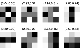
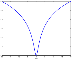
Figure 1: Discriminatively trained FoE prior with the Lorentzian penalty function. (a) the learned filters. The first number in the bracket is weight $\theta_{i}$ and the second one is the norm of the filter $k_{i}$. (b) the corresponding Lorentzian penalty function derived from the Student-t distribution.

(a) Original ($510\times 510$)

(b) Low resolution input ($170\times 170$)

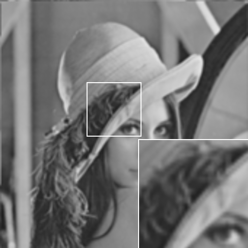
(c) bicubic interpolation (26.62/80.20)

(d) MMSE with (II.2) (32.93/90.34)

(e) MAP with (II.2) (33.16/90.97)

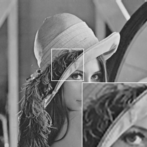
(f) MAP with (III.6) (33.52/91.44)

Figure 2: Single image super resolution results for the noise-free “Lena” image ($\times 3$) with different algorithms. The results are evaluated in terms of PSNR and SSIM ($\times 100$) index.

We also evaluated the performance of the MAP inference in the presence of noise. For the cases of mild Gaussian noise, the results of the MAP inference with two different FoE image prior models are shown in Table II, together with the results of the MMSE based model. Note that this is a direct comparison to TABLE III of [20]. Again, one can see that the MAP estimate with the same FoE model (i.e., (II.2)) works equally well, and it leads to better results with our discriminatively trained FoE prior (III.6).

For the MAP estimate based SR model (II.4), we need to search an optimal $\lambda$ for each case. For the noise-free image SR task, we use a relative large $\lambda=200$, and for the SR tasks with Gaussian noise, we find the following empirical choice (1) $\lambda=3,\text{if}~{}\sigma=1$, (2) $\lambda=1,\text{if}~{}\sigma=2$, and (3) $\lambda=0.5,\text{if}~{}\sigma=3$, generally works well.

Run time: We run the inference algorithms on a server with Inter(R) Xeon(R) CPU E5-2680 v2 @ 2.80GHz. For the SR task of upsampling an image of size $85\times 85$ to the size of $255\times 255$, the average computation time per iteration of the MMSE-based algorithm is 87s. Typically, the MMSE estimate takes 100 iterations, and therefore for this SR task, it requires about $\sim$2.4h, making this approach hardly appealing for practical application.

In contrast, the MAP inference is much faster. The average computation time per iteration of the MAP inference is 0.039s in the case of the Student-t based FoE prior (III.6). Typically, it takes 150$\sim$200 iterations to solve the resulting non-convex minimization problem. As a consequence, the MAP inference with the Student-t based FoE prior is able to accomplish the same SR task in 7s, which is dramatically faster than the MMSE inference ($\sim$2.4h). Implementation will be publicly available at the author’s homepage (http://www.icg.tugraz.at/Members/Chenyunjin).

Moreover, as demonstrated in our previous works [1, 2], the MAP inference of the FoE prior based models can be easily implemented on GPU for parallel computation, which can generally obtain an approximate speedup factor of $40\times$.

III-C Comparison to state-of-the-art SR approaches

In order to conduct a comprehensive evaluation for the MAP based SR model, we further compared it with current state-of-the-art SR approaches: the sparse coding (SC) based approach [17], the K-SVD based method [18], the ANR (Anchored Neighborhood Regression) based method [15] and deep convolutional network based method - SR-CNN [3]. In order to perform a fair comparison with these methods, we strictly obey the same test protocols as in [15]. We download the source codes from the authors’ websites, and use the recommended parameters by the authors. We used the same test sets - Set14 and Set5 to evaluate the upscaling factor of 3.

For the MAP based SR model, we incorporated a FoE prior model with larger filter size and more filters (shown in Figure 3, 48 filters of size $7\times 7$), which is trained in [2]. Replacing the FoE prior model shown in Figure 1 with this new FoE model having increased model capacity can improve the performance of the MAP based SR model.

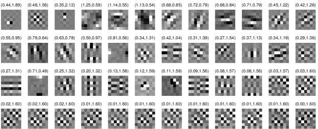
Figure 3: 48 learned filters of size $7\times 7$ exploited in our MAP based SR model.

Set14 images	Bicubic	SC	K-SVD	ANR	SR-CNN	$\text{MAP}_{7\times 7}$
baboon	23.21/54.39	23.47/58.78	23.52/58.99	23.56/59.90	23.60/60.35	23.58/61.50
barbara	26.25/75.31	26.39/76.33	26.76/78.16	26.69/78.11	26.66/78.10	26.43/78.30
bridge	24.40/64.83	24.82/69.21	25.02/69.64	25.01/70.12	25.07/70.50	25.13/71.91
coastguard	26.55/61.49	27.02/63.93	27.15/65.40	27.08/65.77	27.20/65.88	27.25/67.04
comic	23.12/69.88	23.90/75.57	23.96/75.48	24.04/76.06	24.39/77.78	24.26/78.36
face	32.82/79.84	33.11/80.11	33.53/81.95	33.62/82.32	33.58/82.14	33.70/82.91
flowers	27.23/80.13	28.25/82.97	28.43/83.75	28.49/84.03	28.97/84.75	28.84/85.58
foreman	31.18/90.58	32.04/91.32	33.19/92.92	33.23/93.01	33.35/93.21	33.83/93.91
lenna	31.68/85.82	32.64/86.48	33.00/87.82	33.08/88.04	33.39/88.27	33.31/88.64
man	27.01/74.95	27.76/77.49	27.90/78.62	27.92/78.90	28.18/79.40	28.15/80.27
monarch	29.43/91.98	30.71/92.90	31.10/93.82	31.09/93.77	32.39/94.50	31.88/94.77
pepper	32.39/86.98	33.32/86.69	34.07/88.63	33.82/88.51	34.35/88.76	34.30/89.15
ppt3	23.71/87.46	24.98/89.18	25.23/91.17	25.03/90.25	26.02/91.94	26.42/93.52
zebra	26.63/79.42	27.95/82.59	28.49/84.09	28.43/84.24	28.87/84.70	26.81/85.42
average	27.54/77.36	28.31/79.54	28.67/80.75	28.65/80.93	29.00/81.45	28.99/82.23
Set5 images	Bicubic	SC	K-SVD	ANR	SR-CNN	$\text{MAP}_{7\times 7}$
baby	33.91/90.39	34.29/90.42	35.08/92.11	35.13/92.25	35.01/92.10	35.10/92.61
bird	32.58/92.56	34.11/93.91	34.57/94.77	34.60/94.88	34.91/94.94	35.07/95.56
butterfly	24.04/82.16	25.58/86.11	25.94/87.70	25.90/87.17	27.58/90.12	26.79/90.31
head	32.88/80.03	33.17/80.24	33.56/82.04	33.63/82.39	33.55/82.15	33.72/82.99
woman	28.56/88.96	29.94/90.37	30.37/91.76	30.33/91.69	30.92/92.36	30.79/92.80
average	30.39/86.82	31.42/88.21	31.90/89.68	31.92/89.68	32.39/90.33	32.29/90.85

TABLE III: Scale $\times 3$ performance in terms of PSNR and SSIM ($\times 100$) index on the Set14 and Set5 datasets. We compare the results of MAP based SR model (48 filters of size $7\times 7$) to representative state-of-the-art SR methods: SC [17], ANR [15], K-SVD [18] and SR-CNN [3].

(a) Original/PSNR (-)

(b) Bicubic/23.71dB/87.46 (-)

(c) SC/24.98dB/89.18 (89.2s)

(d) ANR/25.03dB/90.25 (1.1s)

(e) K-SVD/25.23dB/91.17 (4.5s)

(f) SR-CNN/26.02dB/91.94 (4.7s)

(g) $\text{MAP}_{7\times 7}$/26.42dB/93.52 (45.3s)

Figure 4: Visual qualitative assessment and quantitative results for “ppt3” image from Set14 with magnification $\times 3$ (best viewed on screen). Note the difference in the highlighted region. The corresponding run time is given in the bracket.

The SR results on Set14 and Set5 are summarized in Table III. We can see that the FoE based SR model with filters of size $7\times 7$ achieves similar average PSNR as the SR-CNN method, and outperforms other competing algorithms. A visual example is shown in Figure 4. In the highlighted region, one can see that our SR method achieve more clear edges than other approaches. In summary our $\text{MAP}_{7\times 7}$ model obtains strongly competitive quality performance to current state-of-the-art SR methods. Furthermore, we also provide the run time of the exploited SR algorithms. Note that all the algorithms are run in Matlab, and therefore, the SR-CNN algorithm is slower than its C++ implementation shown in [3].

In order to illustrate the convergence properties of the iPiano algorithm used to solve the MAP-based SR problem, in Figure 5 we present the energy curve associated with the SR task for the “ppt3”image shown in Figure 4.

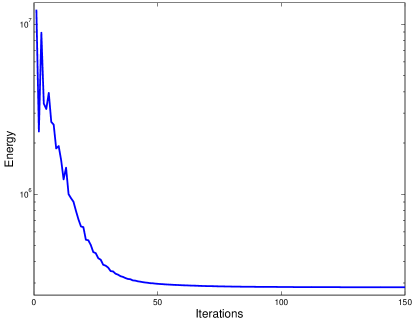
Figure 5: Energy curve of the iPiano algorithm used to solve the SR problem for the image “ppt3” shown in Figure 4.

IV Discussion and Conclusion

In the context of higher-order MRF based models, it is generally true that the MAP estimate, which only seeks for the posterior mode, could not generally exploit the full potential offered by the probabilistic modeling, while the MMSE estimate, which directly draw samples from the probability model, should be more powerful. On the other hand, it is well-known that the sampling based MMSE estimation is very slow, making the corresponding methods hardly appealing for practical applications if one has to stick to the MMSE inference.

In this paper, we have concentrated on the higher-order MRFs based SR problem, and evaluated the performance of the MAP estimate in inference. We found that the MAP estimate can work equally well compared to MMSE in the presence of the same FoE prior, despite of the non-convexity of the resulting optimization problem. We believe the reason is two-folds: first, the exploited iPiano algorithm which is an effective non-convex optimization algorithm, helps us reach the MAP mode in a short time; secondly, in practice one is not able to obtain an accurate solution for the MMSE estimate. In addition, we found that the performance of MAP estimate can be further boosted by using discriminatively trained FoE prior models. As a consequence, the resulting $\text{MAP}_{7\times 7}$ model, which involves 48 filters of size $7\times 7$ can lead to strongly competitive results to very recent state-of-the-art SR methods. Therefore, concerning the higher-order MRFs based SR task, we suggest to exploit the MAP estimate for inference because there is no performance loss by using this simpler inference criterion while it has an obvious advantage of high efficiency.

Furthermore, it is notable to point out that the findings about the MAP estimate presented in this paper strengthen our arguments drawn based on the Gaussian denoising problem in our previous works [1, 2]. We have show in [1, 2] that the MAP-based denoising model with our discriminatively trained FoE prior leads to the best results among the MRF-based systems, including MMSE based models. Therefore, we believe that MAP-based denoising model does not perform well in previous works, e.g., [13, 12] just because they have not obtained a good FoE prior well-suited for the MAP inference.

In summary, we believe that in the context of higher-order MRF image prior based modeling for image restoration problems, it is a better choice to make use of the MAP estimate, together with the discriminatively trained FoE prior.

References

- [1] Y. Chen, T. Pock, R. Ranftl, and H. Bischof. Revisiting loss-specific training of filter-based mrfs for image restoration. In GCPR, pages 271–281, 2013.
- [2] Y. Chen, R. Ranftl, and T. Pock. Insights into analysis operator learning: From patch-based sparse models to higher order MRFs. IEEE Transactions on Image Processing, 23(3):1060–1072, 2014.
- [3] C. Dong, C. C. Loy, K. He, and X. Tang. Learning a deep convolutional network for image super-resolution. In Computer Vision–ECCV 2014, pages 184–199. Springer, 2014.
- [4] Q. Gao and S. Roth. How well do filter-based MRFs model natural images? In DAGM/OAGM Symposium, pages 62–72, 2012.
- [5] C. D. Herrera, J. Kannala, P. Sturm, and J. Heikkila. A learned joint depth and intensity prior using markov random fields. In 3DTV-Conference, 2013 International Conference on, pages 17–24. IEEE, 2013.
- [6] P. Kohli, P. H. Torr, et al. Robust higher order potentials for enforcing label consistency. International Journal of Computer Vision, 82(3):302–324, 2009.
- [7] S. Z. Li. Markov random field modeling in computer vision. Springer-Verlag New York, Inc., 1995.
- [8] Y. Nesterov. Introductory lectures on convex optimization: A basic course, volume 87. Springer, 2004.
- [9] T.-V. Nguyen, N. Pham, T. Tran, and B. Le. Higher order conditional random field for multi-label interactive image segmentation. In Computing and Communication Technologies, Research, Innovation, and Vision for the Future (RIVF), 2012 IEEE RIVF International Conference on, pages 1–4. IEEE, 2012.
- [10] P. Ochs, Y. Chen, T. Brox, and T. Pock. iPiano: Inertial Proximal Algorithm for Nonconvex Optimization. SIAM Journal on Imaging Sciences, 7(2):1388–1419, 2014.
- [11] S. Roth and M. J. Black. Fields of experts. International Journal of Computer Vision, 82(2):205–229, 2009.
- [12] K. G. G. Samuel and M. Tappen. Learning optimized map estimates in continuously-valued MRF models. In CVPR, 2009.
- [13] U. Schmidt, Q. Gao, and S. Roth. A generative perspective on MRFs in low-level vision. In CVPR, pages 1751–1758, 2010.
- [14] U. Schmidt, K. Schelten, and S. Roth. Bayesian deblurring with integrated noise estimation. In Computer Vision and Pattern Recognition (CVPR), 2011 IEEE Conference on, pages 2625–2632. IEEE, 2011.
- [15] R. Timofte, V. De, and L. V. Gool. Anchored neighborhood regression for fast example-based super-resolution. In Computer Vision (ICCV), 2013 IEEE International Conference on, pages 1920–1927. IEEE, 2013.
- [16] X. Wang, C. Hou, L. Pu, and Y. Hou. A depth estimating method from a single image using FoE CRF. Multimedia Tools and Applications, pages 1–16, 2014.
- [17] J. Yang, J. Wright, T. S. Huang, and Y. Ma. Image super-resolution via sparse representation. Image Processing, IEEE Transactions on, 19(11):2861–2873, 2010.
- [18] R. Zeyde, M. Elad, and M. Protter. On single image scale-up using sparse-representations. In Curves and Surfaces, pages 711–730. Springer, 2012.
- [19] H. Zhang and Y. Zhang. Bayesian image separation with natural image prior. In Image Processing (ICIP), 2012 19th IEEE International Conference on, pages 2097–2100. IEEE, 2012.
- [20] H. Zhang, Y. Zhang, H. Li, and T. S. Huang. Generative bayesian image super resolution with natural image prior. Image Processing, IEEE Transactions on, 21(9):4054–4067, 2012.
- [21] B. Zhao, W. Zhang, H. Ding, and H. Wang. Non-blind image deblurring from a single image. Cognitive Computation, 5(1):3–12, 2013.