Quantum Limit in a Magnetic Field for Triplet Superconductivity in a Quasi-One-Dimensional Conductor

Abstract

We theoretically consider the upper critical magnetic field, perpendicular to a conducting axis in a triplet quasi-one-dimensional superconductor. In particular, we demonstrate that, at high magnetic fields, the orbital effects against superconductivity in a magnetic field are reversible and, therefore, superconductivity can restore. It is important that the above mentioned quantum limit can be achieved in presumably triplet quasi-one-dimensional superconductor Li_0.9Mo₆O₁₇ [J.-F. Mercure et al., Phys. Rev. Lett. 108, 187003 (2012)] at laboratory available pulsed magnetic fields of the order of $H=500-700\ T$.

High magnetic field properties of quasi-one-dimensional (Q1D) conductors and superconductors have been intensively studied since the discovery of the Field-Induced Spin-Density-Wave (FISDW) cascade of phase transitions [1-4]. Note that the FISDW phenomenon, experimentally discovered in the (TMTSF)₂X compounds [1,2], where X=ClO₄ and X=PF₆, was historically the first one which was successfully explained in terms of quasi-classical $3D\rightarrow 2D$ dimensional crossover in high magnetic fields [3,5-7]. At present, it has been established that different kinds of quasi-classical dimensional crossovers in a magnetic field are responsible for such unusual phenomena in layered Q1D conductors as the Field-Induced Charge-Density-Wave (FICDW) phase transitions [3,5,8,9], Danner-Kang-Chaikin oscillations [3,10], Lebed Magic Angles [3,11,12], and Lee-Naughton-Lebed oscillations [3,13-16]. Note that a characteristic property of the quasi-classical dimensional crossovers is that the typical ”sizes” of electron trajectories in a magnetic field are much lager than the inter-plane or inter-chain distances in layered Q1D conductors.

On the other hand, a different type of dimensional crossovers in a magnetic field - the so-called quantum dimensional crossover [3] - was suggested in Ref.[17] to describe magnetic properties of a superconducting phase. More specifically, it was shown [17-22] that, at high enough magnetic fields, the typical ”sizes” of electron trajectories become of the order of inter-plane distances and superconductivity can restore as a pure 2D phase. Note that the above mentioned conclusion is valid only for some triplet superconducting phases which are not sensitive to the Pauli paramagnetic effects in a magnetic field. Due to this reason, Q1D superconductors (TMTSF)₂X were considered for many years to be the best candidates for this Reentrant Superconductivity (RS) phenomenon, since triplet superconducting pairing was suggested [23,24] to exist in these materials. Recently, it has been shown [25,22,26] that d-wave singlet superconducting phase is more likely to exist in the (TMTSF)₂ClO₄, therefore, the RS phenomenon experimentally reveals itself in this compound only as the hidden RS phase [22]. As to the superconductor (TMTSF)₂PF₆, the existing experimental data about nature of superconducting pairing in this compound are still controversial [3]. In this difficult situation, it is important that a new strong candidate for triplet superconducting pairing - the Q1D superconductor Li_0.9Mo₆O₁₇ - has been recently proposed [27-29]. In particular, it has been shown in Refs.[28,29] that a quantitative description by triplet scenario of superconductivity, with a magnetic field applied along the conducting axis, can account for the experimental field that exceeds the so-called Clogston-Chandrasekhar paramagnetic limit [30] by five times [27].

The goal of our Letter is to show theoretically that triplet superconductivity scenario can be tested in the Li_0.9Mo₆O₁₇ superconductor in ultra-high magnetic fields of the order of $H\simeq 500-700\ T$, where triplet superconductivity is shown to restore with transition temperature $T^{*}_{c}\simeq 0.75\ T_{c}\simeq 1.4-1.7\ K$. Note that the suggested effect is different from the RS phenomenon [17-22] since we consider a magnetic field, which has non-zero out-off conducting plane component. Therefore, at high magnetic fields, $3D\rightarrow 2D$ crossover [17,3] does not happen. Instead, quantum $3D\rightarrow 1D$ dimensional crossover happens which, to the best of our knowledge, has not been considered and studied so far. We call such crossover $Q1D\rightarrow 1D$ quantum limit (QL) [31]. [Note that below we apply the Fermi liquid approach to the Q1D transition-metal oxide Li_0.9Mo₆O₁₇. Validity of the Fermi liquid picture as well as Q1D nature of electron spectrum in this conductor have been firmly established in Refs.[27-29].]

First, let us demonstrate the suggested in the Letter QL superconductivity phenomenon using qualitative arguments. Below, we consider electron spectrum of a Q1D conductor in a tight-binding approximation,

$$\epsilon({\bf p})=-2t_{x}\cos(p_{x}a_{x})-2t_{y}\cos(p_{y}a_{y})-2t_{z}\cos(p_{z}a_{z}),$$ (1)

where $t_{x}\gg t_{y}>t_{z}$ are overlap integrals of the electron wave functions along ${\bf x}$, ${\bf y}$, and ${\bf z}$ crystallographic axes, respectively. Since $t_{x}\gg t_{y},t_{z}$, the electron spectrum (1) corresponds to two slightly deformed pieces of the Fermi surface (FS) and can be linearized near $p_{x}\simeq\pm p_{F}$,

$$\epsilon({\bf p})=\pm v_{F}(p_{x}\mp p_{F})-2t_{y}\cos(p_{y}a_{y})-2t_{z}\cos(p_{z}a_{z}),$$ (2)

(see Fig.1) where $p_{F}$ and $v_{F}$ are the Fermi momentum and Fermi velocity, respectively. In a magnetic field, perpendicular to the conducting axis,

$${\bf H}=(0,\cos\alpha,\sin\alpha)H,\ {\bf A}=(0,-\sin\alpha,\cos\alpha)Hx,$$ (3)

(see Fig.2) it is possible to write quasi-classical equations of electron motion,

$$\frac{d{\bf p}}{dt}=\bigl{(}\frac{e}{c}\bigl{)}[{\bf v({\bf p})}\times{\bf H}],$$ (4)

in the following way:

$$\frac{d(p_{z}a_{z})}{dt}=\omega_{z}(\alpha)t,\ \ \frac{d(p_{y}a_{y})}{dt}=-\omega_{y}(\alpha)t,$$ (5)

where

$$\omega_{y}(\alpha)=ev_{F}a_{y}H\sin\alpha/c,\ \ \omega_{z}(\alpha)=ev_{F}a_{z}H\cos\alpha/c.$$ (6)

Since electron velocity components can be expressed as functions of time,

$$v_{y}(p_{y})=\partial\epsilon({\bf p})/\partial p_{y}=-2t_{y}a_{y}\sin[\omega_{y}(\alpha)t]\ ,$$

$$v_{z}(p_{z})=\partial\epsilon({\bf p})/\partial p_{z}=2t_{z}a_{z}\sin[\omega_{z}(\alpha)t]\ ,$$ (7)

their trajectories in a real space are described by the following equations:

$$y=l_{y}(\alpha)a_{y}\cos[\omega_{y}(\alpha)t],\ l_{y}(\alpha)=2t_{y}/\omega_{y}(\alpha),$$

$$z=-l_{z}(\alpha)a_{z}\cos[\omega_{z}(\alpha)t],\ l_{z}(\alpha)=2t_{z}/\omega_{z}(\alpha)\ .$$ (8)

As directly follows from Eq.(8), electron motion in a real space in the magnetic field (3) is free along the conducting axes and periodic and restricted perpendicular to the axes. If the magnetic field is strong enough,

$$H\gg H^{*}=\max\biggl{\{}\frac{2t_{y}c}{ev_{F}a_{y}\sin\alpha}\ ,\frac{2t_{z}c}{ev_{F}a_{z}\cos\alpha}\biggl{\}}\ ,$$ (9)

then electron motion in perpendicular directions becomes localized on the conducting axes. This fact is directly seen from Eqs.(8),(9) since the characteristic ”sizes” of electron trajectories, $l_{y}(\alpha)\ a_{y}$ and $l_{z}(\alpha)\ a_{z}$, become less than the corresponding inter-chain distances, $a_{y}$ and $a_{z}$. In this case, electron motion is ”one-dimentionalized” and, as we show below, the Cooper instability restores superconducting phase. [Note that the suggested above localization of the Q1D electrons (2) on conducting chains is completely different from another possible phenomenon - electron localization in unreasonable high magnetic fields, which correspond to a flux quantum per unit cell.]

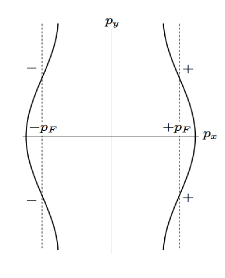
Figure 1: Q1D Fermi surface consists of two slightly corrugated sheets extending in the $z$-direction. The triplet superconducting order parameter changes its sign on the two sheets of the Q1D Fermi surface.

Below, we study the QL superconductivity phenomenon by means of quantitative quantum mechanical methods appropriate for the problem under consideration. In a particular, in the magnetic field (3), we use the Peierls substitution method [5], based on the Fermi liquid description of Q1D electrons (2):

$$p_{x}\mp p_{F}\rightarrow\mp i(d/dx),\ p_{y}a_{y}\rightarrow p_{y}a_{y}-\omega_{y}(\alpha)/v_{F},$$

$$p_{z}a_{z}\rightarrow p_{z}a_{z}+\omega_{z}(\alpha)/v_{F}.$$ (10)

As a result, the Schrödinger-like equation for electron wave functions in the mixed $(p_{y},p_{z},x)$-representation can be written as:

$$\biggl{\{}\mp iv_{F}\frac{d}{dx}-2t_{y}\cos\biggl{[}p_{y}a_{y}-\frac{\omega_{y}(\alpha)}{v_{F}}x\biggl{]}-2t_{z}\cos\biggl{[}p_{z}a_{z}$$

$$+\frac{\omega_{z}(\alpha)}{v_{F}}x\biggl{]}\biggl{\}}\psi_{\epsilon}^{\pm}(p_{y},p_{z},x)=\delta\epsilon\ \psi_{\epsilon}^{\pm}(p_{y},p_{z},x),$$ (11)

where electron energy is counted from the Fermi energy, $\delta\epsilon=\epsilon-\epsilon_{F}$, $\epsilon_{F}=p_{F}v_{F}$. Note that in Eq.(11) we disregard electron spin since we consider below such triplet superconducting phase where the Pauli paramagnetic effects do not reveal themselves. It is important that Eq.(11) can be solved analytically:

$$\psi_{\epsilon}^{\pm}(p_{y},p_{z},x)=\exp\biggl{(}\frac{\pm i\delta\epsilon x}{v_{F}}\bigg{)}\exp\biggl{\{}\pm 2il_{y}(\alpha)\biggl{(}\sin\biggl{[}p_{y}a_{y}$$

$$-\frac{\omega_{y}(\alpha)}{v_{F}}x\biggl{]}-\sin[p_{y}a_{y}]\biggl{)}\biggl{\}}\exp\biggl{\{}\mp 2il_{z}(\alpha)\biggl{(}\sin\biggl{[}p_{z}a_{z}$$

$$-\frac{\omega_{z}(\alpha)}{v_{F}}x\biggl{]}-\sin[p_{z}a_{z}]\biggl{)}\biggl{\}}.$$ (12)

Since electron wave functions are known (12), we can define the finite temperatures Green’s functions by means of the standard procedure [32]:

$$g_{i\omega_{n}}^{\pm}(p_{y},p_{z};x,x_{1})=\int^{+\infty}_{-\infty}d(\delta\epsilon)[\psi^{\pm}_{\epsilon}(p_{y},p_{z};x)]^{*}$$

$$\times\psi^{\pm}_{\epsilon}(p_{y},p_{z};x_{1})/(i\omega_{n}-\delta\epsilon),$$ (13)

where $\omega_{n}$ is the so-called Matsubara frequency.

In the Letter, we consider the following gapless triplet superconducting order parameter in the Li_0.9Mo₆O₁₇, which, as shown in Refs.[28,29], well satisfies the experimental data [27]:

$$\hat{\Delta}(p_{x},x)=\hat{I}\ sgn(p_{x})\ \Delta(x),$$ (14)

where $\hat{I}$ is a unit matrix in spin-space, $sgn(p_{x})$ changes sign of the triplet superconducting order parameter on two slightly corrugated sheets of the Q1D FS (2) (see Fig.1).

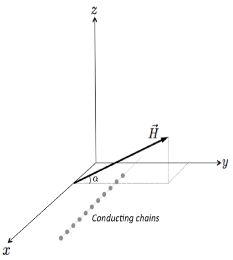
Figure 2: The magnetic field makes an angle $\alpha$ with respect to the $y$ axis, perpendicular to the conducting chains.

We use the Gor’kov’s equations for unconventional superconductivity [33,34] to obtain the so-called gap equation for superconducting order parameter $\Delta(x)$. As a result, we derive the following equation:

$$\Delta(x)=\frac{g}{2}\int_{|x-x_{1}|>d}\frac{2\pi Tdx_{1}}{v_{F}\sinh\bigl{[}\frac{2\pi T|x-x_{1}|}{v_{F}}\bigl{]}}\ \Delta(x_{1})$$

$$\times J_{0}\biggl{\{}4l_{y}(\alpha)\sin\biggl{[}\frac{\omega_{y}(\alpha)(x-x_{1})}{2v_{F}}\bigg{]}\sin\biggl{[}\frac{\omega_{y}(\alpha)(x+x_{1})}{2v_{F}}\bigg{]}\biggl{\}}$$

$$\times J_{0}\biggl{\{}4l_{z}(\alpha)\sin\biggl{[}\frac{\omega_{z}(\alpha)(x-x_{1})}{2v_{F}}\bigg{]}\sin\biggl{[}\frac{\omega_{z}(\alpha)(x+x_{1})}{2v_{F}}\bigg{]}\biggl{\}},$$ (15)

where $g$ is the electron coupling constant, and $d$ is the cutoff distance.

Note that the QL superconductivity phenomenon is directly seen from Eq.(15). Indeed, at high enough magnetic fields (9), the parameters $l_{y}(\alpha)$ and $l_{z}(\alpha)$ become less than 1. Under this condition, arguments of the Bessel functions in Eq.(15) go to zero and superconducting transition temperature goes to its value in the absence of magnetic field, $T_{c}$:

$$\lim_{H\rightarrow\infty}T^{*}_{c}(H)\rightarrow T_{c}.$$ (16)

It is also important that Eq.(15) predicts that superconductivity in a triplet Q1D superconductor without impurities can survive at any magnetic fields, including magnetic fields lower than that in Eq.(9). Nevertheless, we point out that for magnetic fields less than (9) superconducting transition temperatures are very low and an account of small amount of impurities would presumably kill the superconducting phase.

For experimental applications of our results, it is important to calculate how quickly superconductivity tends to $T_{c}(0)$ in Eq.(16). For this purpose, we expand each Bessel function in Eq.(15) to the second order with respect to the small parameters $l_{y}(\alpha),l_{z}(\alpha)\ll 1$:

$$J_{0}\{...\}\ J_{0}\{...\}\simeq 1$$

$$-4l^{2}_{y}(\alpha)\sin^{2}\biggl{[}\frac{\omega_{y}(\alpha)(x-x_{1})}{2v_{F}}\bigg{]}\sin\biggl{[}\frac{\omega_{y}(\alpha)(x+x_{1})}{2v_{F}}\bigg{]}$$

$$-4l^{2}_{z}(\alpha)\sin^{2}\biggl{[}\frac{\omega_{z}(\alpha)(x-x_{1})}{2v_{F}}\bigg{]}\sin\biggl{[}\frac{\omega_{z}(\alpha)(x+x_{1})}{2v_{F}}\bigg{]}\ .$$ (17)

In the second approximation with respect to the small parameters $l_{y}(\alpha)$ and $l_{z}(\alpha)$ it is possible to use in the integral gap equation (15),(17) the following trial function:

$$\Delta(x)=\Delta(y)=const.$$ (18)

In this approximation, we can also average Eq.(15),(17) over variable $x+x_{1}$ and after using the following formula,

$$\frac{1}{g}=\int_{d}^{+\infty}\frac{2\pi T_{c}dz}{\sinh\biggl{(}\frac{2\pi T_{c}z}{v_{F}}\biggl{)}},$$ (19)

we obtain:

$$T_{c}^{*}(H)=T_{c}\biggl{\{}1-l^{2}_{y}(\alpha)\ln\biggl{[}\frac{\gamma\omega_{y}(\alpha)}{\pi T_{c}}\biggl{]}-l^{2}_{z}(\alpha)\ln\biggl{[}\frac{\gamma\omega_{z}(\alpha)}{\pi T_{c}}\biggl{]}\biggl{\}},$$ (20)

where $\gamma$ is the Euler constant. From Eq.(20) it is directly seen that, at high enough magnetic fields (9), Eq.(16) is valid.

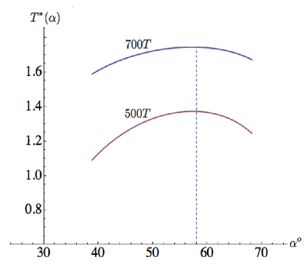
Figure 3: The QL superconducting transition temperature dependence of the angle, $\alpha$, for magnetic fields of $500T$ and $700T$. Both maximums occur at an angle of $\alpha\approx 58^{o}$. The maximum temperature at $700T$ is approximately $1.7K$.

For experimental applications of our results it is important to estimate the value of $T_{c}^{*}(H)$ in Eq.(20) for the presumably triplet [27-29] Q1D superconductor Li_0.9Mo₆O₁₇ in experimental range of magnetic fields. Using known values of the parameters $a_{y}$, $a_{z}$, $v_{F}$, $t_{y}$, and $t_{z}$ (see Table 1 in Ref.[28]), it is possible to find that

$$\omega_{y}(H=1\ T,\alpha=\pi/2)=0.76\ K,$$

$$\omega_{z}(H=1\ T,\alpha=0)=0.57\ K,$$

$$l_{y}(H=1\ T,\alpha=\pi/2)=116,$$

$$l_{z}(H=1\ T,\alpha=0)=49\ .$$ (21)

Our next step is to input these parameters into Eq.(20) and to plot $T_{c}^{*}(\alpha)$ as a function of $\alpha$ at given $H$. [We recall that superconducting transition temperature in the absence of a magnetic field is equal to $T_{c}=2.2\ K$.] In Fig.3, we plot angular dependence of the QL superconducting phase transition temperature for two values of a magnetic field, $H=500\ T$ and $H=700\ T$. As seen from Fig.3, the maximum values of $T^{*}_{c}(H)$ corresponds to angle $\alpha^{*}\simeq 58^{0}$ in both cases with highest $T^{*}_{c}(H=700\ T)\simeq 1.7\ K$. Note that region of validity of Eq.(20) corresponds to the condition $|T^{*}_{c}(H)-T_{c}|\ll T_{c}$, therefore, we conclude that Fig.3 correctly represents calculated transition temperature near its maximums for both values of the magnetic field. Note that magnetic fields of the order of $H=500,\ 700\ T$ are currently experimentally available as distructive pulsed magnetic fields.

In the Letter, we have demonstrated that superconductivity can be restored in a triplet Q1D superconductor in a magnetic field, perpendicular to its conducting axis, as the Quantum Limit (QL) superconducting phase. It happens if a magnetic field is high enough [see Eq.(9)] to localize electrons on conducting chains of a Q1D conductor. Note that such ”one-dimensionalization” of Q1D electron spectrum promotes also the FISDW instability [5-7] and non-Fermi-liquid properties [3]. Therefore, we suggest that superconducting instability is a leading one and that electron wave function delocalizations between adjacent chains are high enough for the Fermi-liquid picture to survive. Note that the FICDW instability [8,9] is not expected in high magnetic fields since the Pauli paramagnetic effects significantly decrease the FICDW transition temperature [35]. We suggest to carry out the corresponding experiment on the presumably triplet superconductor Li_0.9Mo₆O₁₇ in feasibly available pulsed magnetic fields of the order of $H=500-700\ T$ and temperatures less than $T^{*}_{c}\simeq 1.4-1.7\ K$. We have also determined the most convenient geometry of the experiment which, as shown, corresponds to inclination angle of $\alpha=58^{0}$ [see Eq.(3) and Fig.2]. It is important that the QL superconductivity phenomenon is not very sensitive to possible deviations of geometry from the most convenient one, as seen from Eq.(20) and Fig.3. If the result of the suggested experiment is positive it will confirm triplet superconductivity scenario [27-29] in the above mentioned compound and for the first time establish surviving of superconductivity in ultra-high magnetic fields.

One of us (A.G.L.) is thankful to N.N. Bagmet and N.E. Hussey for useful discussions. This work was supported by the NSF under Grant No DMR-1104512.

^∗Also at: L.D. Landau Institute for Theoretical Physics, RAS, 2 Kosygina Street, Moscow 117334, Russia.

References

- (1) P.M. Chaikin, Mu-Yong Choi, J.F. Kwak, J.S. Brooks, K.P. Martin, M.J. Naughton, E.M. Engler, and R.L. Greene, Phys. Rev. Lett. 51, 2333 (1983).
- (2) M. Ribault, D. Jerome, J. Tuchendler, C. Weyl, and K. Bechgaard, J. Phys. (Paris) Lett, 44, L-953 (1983).
- (3) The Physics of Organic Superconductors and Conductors, edited by A.G. Lebed (Springer, Berlin, 2008).
- (4) T. Ishiguro, K. Yamaji, and G. Saito, Organic Superconductors, (Springer, Berlin, 1998).
- (5) L.P. Gor’kov and A.G. Lebed, J. Phys. (Paris), Lett. 45, L-433 (1984).
- (6) M. Heritier, G. Montambaux, and P. Lederer, J. Phys. (Paris), Lett. 45, L-943 (1984).
- (7) A.G. Lebed, Sov. Phys. JETP, 62, 595 (1985).
- (8) D. Zanchi, A. Bjelis, and G. Montambaux, Phys. Rev. B 53, 1240 (1996).
- (9) A.G. Lebed, Phys. Rev. Lett. 103, 046401 (2009).
- (10) M. Danner, W. Kang, and P. M. Chaikin, Phys. Rev. Lett. 72, 3714 (1994).
- (11) A.G. Lebed, JETP Lett. 43, 174 (1986).
- (12) A.G. Lebed and P. Bak, Phys. Rev. Lett. 63, 1315 (1989).
- (13) M.J. Naughton, I.J. Lee, P.M. Chaikin, and G.M. Danner, Synth. Met. 85, 1481 (1997).
- (14) H. Yoshino, K. Saito, H. Nishikawa, K. Kikuchi, K. Kobayashi, and I. Ikemoto, J. Phys. Soc. Jpn. 66, 2248 (1997).
- (15) I.J. Lee and M.J. Naughton, Phys. Rev. B 57, 7423 (1998).
- (16) A.G. Lebed and M.J. Naughton, Phys. Rev. Lett. 91, 187003 (2003).
- (17) A.G. Lebed, JETP Lett. 44, 114 (1986).
- (18) N. Dupuis, G. Montambaux, and C.A.R. Sa de Melo, Phys. Rev. Lett. 70, 2613 (1993).
- (19) I.J. Lee, M.J. Naughton, G.M. Danner, and P.M. Chaikin, Phys. Rev. Lett. 78, 3555 (1997).
- (20) V.P. Mineev, J. Phys. Soc. Jpn. 69, 3371 (2000).
- (21) N. Belmechri, G. Abramovici and M. Heritier, Europhys. Lett. 82, 47009 (2008).
- (22) A.G. Lebed, Phys. Rev. Lett. 107, 087004 (2011); Physica B 407, 1803 (2012); JETP Lett. 94, 382 (2011).
- (23) A.A. Abrikosov, J. Low Temp. Phys., 53, 359 (1983).
- (24) I.J. Lee, S.E. Brown, W.G. Clark et al., Phys. Rev. Lett. 88, 017004 (2002).
- (25) J. Shinagawa, Y. Kurosaki, F. Zhang et al., Phys. Rev. Lett. 98, 147002 (2007).
- (26) C. Bourbonnais and A. Sedeki, Phys. Rev. B 80, 085105 (2009).
- (27) J.-F. Mercure, A.F. Bangura, Xiaofeng Xu, N. Wakeham, A. Carrington, P. Walmsley, M. Greenblatt, and N.E. Hussey, Phys. Rev. Lett., 108, 187003 (2012).
- (28) A.G. Lebed and O. Sepper, Phys. Rev. B 87, 100511(R) (2013).
- (29) O. Sepper and A.G. Lebed, Phys. Rev. B 88, 094520 (2013).
- (30) A.M. Clogston, Phys. Rev. Lett. 9, 266 (1962); B.S. Chandrasekhar, Appl. Phys. Lett. 1, 7 (1962).
- (31) We also stress that the suggested in this Letter QL is qualitatively different from QL for isotropic 3D electrons, suggested in M. Razolt and Z. Tesanovic, Rev. Mod. Phys. 64, 709 (1992).
- (32) A.A. Abrikosov, L.P. Gor’kov, and I.E. Dzyaloshinski, Methods of Quantum Field Theory in Statistical Physics (Dover, New York, 1975).
- (33) M. Sigrist and K. Ueda, Rev. Mod. Phys. 63, 239 (1991).
- (34) A.G. Lebed and K. Yamaji, Phys. Rev. Lett. 80, 2697 (1998).
- (35) X. Xu, A.F. Bangura, J.G. Analytis, J.D. Fletcher, M.M.J. French, N. Shannon, J. He, S. Zhang, D. Mandrus, R. Jin, and N.E. Hussey, Phys. Rev. Lett. 102, 206602 (2009).