The definition of environment and its relation to the quenching of galaxies at z=1-2 in a hierarchical Universe.

Abstract

A well calibrated method to describe the environment of galaxies at all redshifts is essential for the study of structure formation. Such a calibration should include well understood correlations with halo mass, and the possibility to identify galaxies which dominate their potential well (centrals), and their satellites. Focusing on z$\sim 1$ and $2$ we propose a method of environmental calibration which can be applied to the next generation of low to medium resolution spectroscopic surveys. Using an up-to-date semi-analytic model of galaxy formation, we measure the local density of galaxies in fixed apertures on different scales. There is a clear correlation of density with halo mass for satellite galaxies, while a significant population of low mass centrals is found at high densities in the neighbourhood of massive haloes. In this case the density simply traces the mass of the most massive halo within the aperture. To identify central and satellite galaxies, we apply an observationally motivated stellar mass rank method which is both highly pure and complete, especially in the more massive haloes where such a division is most meaningful. Finally we examine a test case for the recovery of environmental trends: the passive fraction of galaxies and its dependence on stellar and halo mass for centrals and satellites. With careful calibration, observationally defined quantities do a good job of recovering known trends in the model. This result stands even with reduced redshift accuracy, provided the sample is deep enough to preserve a wide dynamic range of density.

1 Introduction

In the widely accepted Lambda-Cold Dark Matter ($\rm\Lambda CDM$) scenario (White & Rees, 1978; Perlmutter et al., 1999) of structure formation, primordial density fluctuations collapse into virialized haloes. Baryons follow the gravitational field of the dark matter giving birth to galaxies which then interact and merge. As a result, galaxies can live in a great variety of different environments possibly impacting their evolution and fate. Indeed, the fraction of passive galaxies, and the fraction of morphologically early-type galaxies, show strong, positive correlations with the local (projected) density of neighbouring galaxies (Dressler 1980; Balogh et al. 1997, 2004; Poggianti et al. 1999; Kauffmann et al. 2004; see also Blanton & Moustakas 2009 for a review). A variety of stripping effects can and do act on galaxies in dense environments (see Boselli & Gavazzi 2006 for a review), for example ram pressure stripping (Gunn & Gott, 1972; Abadi et al., 1999), strangulation (Larson et al., 1980), and tidal stripping (Keel et al., 1985; Dekel et al., 2003; Diemand et al., 2007; Villalobos et al., 2013). However, the correlation of galaxy properties with environment can also reflect differences in the merger and growth history of (particularly massive) galaxies, driving correlations with halo, stellar and bulge mass but also (indirectly) with density (e.g. Woo et al., 2013; Wetzel et al., 2013; Wilman et al., 2013; Hirschmann et al., 2014).

At $z\sim 1-2.5$, galaxies are in a stage of maximum growth via star formation (Madau et al., 1996; Elbaz et al., 2007; Rodighiero et al., 2011) and mergers. To first order, this happens because gas and galaxies track the accretion of dark matter (see e.g. Lilly et al., 2013; Saintonge et al., 2013) and thus is a consequence of rapid early structure growth. Thus most satellites at this epoch are experiencing a dense surrounding medium for the first time, and gas stripping can have a dramatic impact on the suppression of active star formation.

However, even at low redshift, where a wealth of multi-wavelength data is available, it is non trivial to disentangle the relative contribution of different physical processes as a function of stellar mass, environment and the hierarchy of a galaxy in its own halo (e.g. being a central or a satellite). It is therefore clear that witnessing the rise and decline of the cosmic star formation activity and its dependencies on environment in the early stages of the life of the Universe is even more challenging. Significant effort has been invested in testing measurements of density in the face of difficult selection and redshift errors at $z\sim 1$ – including survey edge effects, magnitude selection, incompleteness and limited redshift accuracy (Cooper et al., 2005; Kovač et al., 2010). These efforts, and the interpretation of resulting correlations of environment with galaxy properties, are hampered by the inhomogeneity of methods used for different surveys and by the lack of calibration to theoretically important parameters such as halo mass.

In the past couple of decades, efforts to model the evolution of galaxies by pasting simple recipes describing baryonic physics onto the hierarchical merger trees of dark matter (DM) haloes in a $\Lambda$CDM Universe (semi-analytical models of galaxy formation, SAMs) have gained momentum and had some success in reproducing the properties of the galaxy population, especially at $z\sim 0$ (see e.g. White & Frenk, 1991; Kauffmann et al., 1993; Cole et al., 1994, 2000; Somerville & Primack, 1999; Bower et al., 2006; Croton et al., 2006; De Lucia & Blaizot, 2007; Monaco et al., 2007; Guo et al., 2011, 2013). Although the predictions of this class of model are still in tension with some observational properties – such as the evolution of low-mass galaxies (Fontanot et al., 2009; Weinmann et al., 2012; Henriques et al., 2013), the properties of satellite galaxies (Weinmann et al., 2009; Boylan-Kolchin et al., 2012; Hirschmann et al., 2014); the baryon fraction on galaxy clusters (McCarthy et al., 2007) – SAMs can be useful to calibrate and test methods to define environment at different redshift.

Our goal is twofold: First, we aim at defining a self-consistent and purely observational parameter space within which the detailed dependence of galaxy properties on their surrounding structure can be evaluated without prejudice. We will thus use mock galaxy catalogues to construct a projected density field evaluated in redshift space, in order to test the impact of different definitions of density and at different redshift accuracy. We also compute a stellar mass rank within an aperture, which provides a purely observational parameter relating to the local gravitational dominance of a particular galaxy. These simple parameters contrast with complementary methods such as the construction of a group catalogue which forces each galaxy into a single halo, using an algorithm with idealized parameters derived from models.

Second, once such trends are established, it is equally important to examine how this contrasts with physical predictions and understand those trends in the context of theoretically important parameters such as halo mass and whether a galaxy is a central or satellite of its halo. We calibrate our observational parameters by examining how they correlate with those accessible in a semi-analytic model.

This two-step process is Bayesian in nature (galaxies have a well defined observational parameter set, while the theoretical parameter calibrations are probabilistic) which is well suited to statistical studies, as well as to the application of selection functions and measurement errors when simulating a real survey. Our definition for what we call “environment” can be equally applied at high or low redshift, although in this paper we focus on high redshift where new opportunities are beginning to open up with low resolution spectroscopic surveys conducted in the NIR (e.g. Brammer et al., 2012). We also concentrate this paper exclusively on the calibration of environment using models and testing our recovery of known trends in the model using our methods. These methods will be applied to observational data in future papers.

There are many ways to describe the density field, e.g. number of neighbours within an adaptive or fixed cylindrical aperture, adaptive smoothing (Park et al., 2007), Voronoi tessellation (Scoville et al., 2013) and shape statistics (Dave et al., 1997).

We focus on a set of simple density measurements using neighbouring galaxies. This is straightforward to correct for incompleteness and calibrate for survey selection and for redshift errors. There are typically two flavours of this method. The first, based on the Nth nearest neighbour (Dressler, 1980; Baldry et al., 2006; Cooper et al., 2006; Poggianti et al., 2008; Brough et al., 2011) correlates only weakly with halo mass (Haas et al., 2012; Muldrew et al., 2012). The second, more sensitive to high-mass over densities, and possibly easier to interpret, is based on the number of galaxies within a fixed aperture (Hogg et al., 2003; Kauffmann et al., 2004; Croton et al., 2005; Gavazzi et al., 2010; Wilman et al., 2010). Recently, Shattow et al. (2013) have demonstrated that the fixed apertures method is more robust across cosmic time, is less sensitive to the viewing angle, and closer to the real over density measured in 3D space than the Nth nearest neighbour. For those reasons, we use this method to quantify the environment.

The paper is structured as follows. In Section 2 we introduce the semi-analytical models used and we discuss the sample selection and the corrections needed to obtain a sample comparable to observations. In Section 3 we present our method describing how to compute the local galaxy density. In Section 4 we present a detailed analysis of correlations between density defined on different scales and halo masses, with a focus on the different behaviour of centrals and satellites. In Section 5 we present an observationally motivated method to identify centrals and satellites and we carefully assess the performances of this method using the models. In Section 6 we test to what extent the tools we have developed are effective in recovering environmental trends on physical properties for model galaxies. We focus on a single property: the fraction of passive galaxies because of its strong environmental dependence in the models. Finally in Section 7 we discuss and summarise the main results of this work.

Throughout the paper we assume a $\rm\Lambda CDM$ cosmology with the following values derived from WMAP7 (Komatsu et al., 2011) observations: $\Omega_{m}=0.272,~{}\Omega_{b}=0.045,~{}\Omega_{\Lambda}=0.728,~{}n=0.961,~{}\sigma_{8}=0.807$ and $h=0.704$.

2 Models

In this study we make use of the latest release of the Munich model as introduced by Guo et al. (2011, hereafter G11) and later updated to WMAP7 cosmology by Guo et al. (2013, hereafter G13). This model takes advantage of a new run of the Millennium N-body simulation (Thomas et al. in prep.) which includes $N=2160^{3}$ particles within a comoving box of size $500h^{-1}$ Mpc on a side and cosmological initial conditions consistent with WMAP7 observational constraints. These are in reasonable agreement with the most recent result from both the WMAP9 (Hinshaw et al., 2013) and the Planck (The Planck Collaboration , 2013) missions. The particle mass resolution is $9.31\times 10^{8}h^{-1}M\odot$, and simulation data are stored at 62 output times. The most significant difference between the assumed cosmological parameters and those used in the original Millennium run (which assumes WMAP1 cosmology) is a lower value of $\sigma_{8}$. This implies a lower amplitude for primordial fluctuations which is partially compensated by a higher value of $\Omega_{m}$. G13 performed a detailed comparison of several statistical properties of the galaxy population in WMAP1 and WMAP7 cosmologies. The impact of a lower $\sigma_{8}$ on the galaxy population was also studied in detail in Wang et al. (2008, using WMAP3 cosmology), and we refer the reader to these papers for the details. G13 model is therefore optimally suited for our purposes due to the combination of the correct cosmology and the large volume.

In order to evaluate the local density around each galaxy, accurate positions of each sub-halo (the main unit hosting a galaxy) are crucial. In G13 main haloes are detected using a standard friends-of-friends (FOF) algorithm. Then each group is decomposed into sub-haloes running the algorithm SUBFIND (Springel et al., 2001), which determines the self-bound structures within an FOF group. Each sub-halo hosts a galaxy. As time goes by, the model follows dark matter haloes after they are accreted onto larger structures. When two haloes merge, the galaxy hosted in the more massive halo is considered the central, and the other becomes a satellite. After infall the haloes experience tidal truncation and stripping (De Lucia et al., 2004; Gao et al., 2004) and their mass is reduced until they fall below the resolution limit of the simulation (20 bound particles, i.e. $2.64\times 10^{10}M_{\odot}$). When this happens the sub-halo is no longer present in the simulation catalog but the galaxy still lives in the main halo (those objects are called orphan galaxies). Its lifetime is set by the dynamical friction formula (see De Lucia et al., 2010) and its position is assigned to the position of the most-bound particle in the sub-halo (this particle being defined at the last time the sub-halo was detected). Once this time has elapsed the galaxy is assumed to merge with the central galaxy of the main halo. Although crude, this assumption reproduces well some observational results like the radial density profile of galaxy clusters (which are dominated by orphan galaxies in the central regions, Gao et al. 2004), and the clustering amplitude on small scales (Wang et al., 2006).

The G13 model is based on earlier versions of the Munich model, e.g. Croton et al. (2006) and De Lucia & Blaizot (2007). It includes prescriptions for gas cooling, star formation, size evolution, stellar and AGN feedback, and metal enrichment. G13 assumes a new and more realistic implementation (compared to the simple model by Mo et al. 1998) for the sizes of gas discs. Both supernovae (SN) and active galactic nuclei (AGN) feedback are implemented. The first implies that massive stars explode as supernovae and the energy released converts a fraction of the cold gas into the hot phase or even expels it from the halo. AGN feedback is implemented following the model by Croton et al. (2006). It is assumed to be caused by ‘radio mode’ outflows from a central black hole that reduces and can completely suppress the cooling of hot gas onto the galaxy. For more details on these prescriptions we refer the reader to G11, G13 and De Lucia & Blaizot (2007).

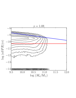
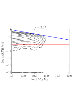
Figure 1: Specific star formation rate ($sSFR$) as a function of $M_{*}$ at redshifts of $1.08$ (left panel) and $2.07$(right panel). The blue line is the main sequence fit from observational data (NMBS, Whitaker et al. 2012). The red line marks the limit we set to define the passive galaxies in the models. The contour levels are log-spaced with the outermost contour at 25 objects and the innermost at $10^{4}$ per bin. We set all galaxies with $\log sSFR<-14$ equal to that value.

It is worth mentioning that current SAMs suffer from an overproduction of low-mass galaxies at high-redshift. Recently, Henriques et al. (2013) presented a new model in which the reincorporation timescales of galactic wind ejecta are a function of halo mass. As a result they obtain a better fit of observed stellar mass functions out to $z\sim 3$. However, because this new prescriptions are not implemented in G13 we perform a statistical correction to the number densities as presented in Sect. 2.1.

In most SAMs the satellite population has been quenched too quickly due to instantaneous stripping of the hot gas (e.g. Weinmann et al., 2006, 2010). G11 proposed a more gentle action of strangulation and ram pressure stripping which are active only when a galaxy falls into the virial radius of a more massive halo. Although this improves the treatment of environmental effects, the fraction of passive galaxies is still significantly overestimated compared to observational results at $z=0$ as shown by Hirschmann et al. (2014). While this discrepancy is reduced in G13, the passive fraction is still too large.

2.1 The model galaxy sample

From the 62 outputs of the simulation, we make use of those at $z=1.08$ and $z=2.07$. We select galaxies above a fixed stellar mass limit of $10^{9.5}M_{\odot}$ in both the redshift snapshots. This limit is high enough to protect us against resolution bias in the models and on the other hand is as deep as the current spectroscopic observations at these redshift can realistically reach. Setting the same mass limit at different redshifts allows us to witness the number density increase as the Universe evolves and we get $\log(n/\rm{Mpc^{3}})=-2.08,-2.28$ at $z=1.08,2.07$ respectively. Those values are higher than the number densities recently obtained by Muzzin et al. (2013) integrating the stellar mass functions (SMFs) from the COSMOS/ULTRAVista observational data ($\log(n/\rm{Mpc^{3}})=-2.19,-2.68$ at $z=1.08,2.07$). Indeed the models fail to match the observed SMFs at $z>1$ by over-predicting the number of galaxies below the characteristic mass ($M_{*}$) of the SMF (Fontanot et al., 2009; Hirschmann et al., 2012; Wang et al., 2012). This discrepancy, which gets worse at higher redshifts, arises in the central galaxy population of intermediate mass haloes, but affects also satellites (as centrals become satellites in a hierarchical Universe). We statistically correct this problem by assigning to each galaxy a weight ($w$) which is the ratio between the predicted and the observed SMFs (i.e. number densities) at the stellar mass of the galaxy. For this correction, the model stellar masses are convolved with a gaussian error distribution with sigma 0.25 dex in order to match the uncertainties on the observed stellar masses. We use the the observed SMFs from Muzzin et al. (2013) because the mass limit of their dataset is well below $M_{*}$ at the redshifts of our interest allowing a robust determination of the faint end slope. Moreover the data are deep enough that the SMFs are not extrapolated to the stellar mass limit we use at $z=1.08$, and extrapolated by only 0.5 dex at $z=2.07$. The weight is then used when computing the local density around each galaxy as presented in Section 3 and when statistical properties of galaxies or of their parent haloes are computed, unless otherwise stated.

To define passive galaxies we make use of the specific star formation rate ($sSFR$), i.e. the star formation rate per unit mass. We set the $sSFR$ limit as follows:

$$sSFR<b/t_{z}$$ (1)

where $b$ is the birthrate parameter $b=SFR/<SFR>$ as defined by Sandage (1986) and $t_{z}$ is the age of the universe at redshift $z$. Inspection of the sSFR distribution in our models revealed there is little, if any, dependence on stellar mass, thus we use the value proposed by Franx et al. (2008): $b=0.3$ (see Figure 1). The $sSFR$ limits are $\sim 5.5\times 10^{-11},~{}{\rm and}~{}9.1\times 10^{-11}~{}\rm yr^{-1}$ at $z=1.08$ and $2.07$ respectively. The quantitative results presented in this paper would slightly change if a different limit is set. None the less the qualitative trends are unchanged.

3 Quantification of environment

For the following analysis, we use model galaxies to reproduce and test different possible measurements of the density on scales ranging from intra-halo to super-halo. First of all we convert one of the comoving axes of the simulation box into a physically motivated redshift. The centre of the box is taken to be at the exact redshift of the snapshot under investigation. We compute the positional offset of each galaxy from the centre and convert this into a redshift offset using a cosmology calculator (Wright, 2006). Then, the effect of peculiar velocities is included to produce redshift distortions. This produces redshifts with a quality similar to high spectral resolution observations (hires-z hereafter). We also create two sets of less accurate redshifts. The first one is obtained by convolving the hires-z with a gaussian error distribution with $\sigma=1000km/s$. This roughly corresponds to the redshift accuracy of low spectral resolution (lowres-z) surveys such as those obtained using slitless spectroscopy on HST (Brammer et al., 2012). Those surveys have the huge advantage of obtaining a redshift for every object in the observed field, reducing the selection bias of pointed spectroscopic surveys and increasing the sampling rate close to $100\%$. The second set is a photometric redshift (photo-z) sample obtained by convolving the hires-z with a gaussian error distribution with $\sigma=5000km/s$. When the redshifts accuracy is decreased, galaxies can be scattered outside the redshift interval (which is set by the size of the simulation box). In those cases we assume a periodic box such that galaxies scattered beyond the maximum redshift are included in the front of the box and viceversa. We make use of those three samples to test the performances of our methods in different scenarios.

In order to obtain measurements of density we apply a method similar to the one described in Wilman et al. (2010). We consider all the galaxies more massive than the limit set in Section 2 and we calculate the projected density of weighted neighbouring galaxies $\Sigma_{r_{i},r_{o}}$ in a combination of annuli centered on these galaxies with inner radii $r_{i}$ and outer radii $r_{o}$. Our set of apertures ranges from 0.25 Mpc to 1.5 Mpc. This allows us enough flexibility to use either a single circular annulus ($r_{i}=0$) or a combination of a circular annulus ($r_{i_{1}}=0$) and an outer annulus that does not overlap with the previous one ($r_{i_{2}}=r_{o_{1}}$). As shown by Wilman et al. (2010) this method allows us to test the correlation between galaxy properties and the density on different scales. For an annulus described by $r_{i}$ and $r_{o}$, the projected density is computed as follows:

$$\Sigma_{r_{i},r_{o}}=\frac{w_{r_{i},r_{o}}}{\pi(r_{o}^{2}-r_{i}^{2})}$$ (2)

where $w_{r_{i},r_{o}}$ is the sum of the weights of neighbouring galaxies living at a physical projected distance $r_{i}\leq r<r_{o}$ from the primary galaxy, and within a rest-frame relative velocity range $\pm dv$. Hereafter, the density in a circle will simply be labelled as $\Sigma_{r_{o}}$. The primary galaxy is not included in the sum, thus isolated galaxies have $\Sigma_{r_{o}}=0$.

The use of weights effectively changes the number of galaxies per halo or aperture in order to match the stellar mass function, without altering the clustering properties of haloes from the simulation. At intermediate to high densities this approach is sufficient to mimic the real universe, while at lower densities there is little dependence of the quantities we study (median halo mass, passive fraction) with density. In the end, the qualitative trends presented in this work are not different if the weights are not applied.

We use the velocity cut at $dv=1500km/s$ for the hires and lowres-z samples. This is indeed adequate for a sample with complete spectroscopic redshift coverage (Muldrew et al., 2012; Shattow et al., 2013), which will be the case for deep field surveys in the near future. Because the photometric redshifts are less accurate, we increase the velocity cut at $dv=7000km/s$, when we use this sample. This keeps the ratio between $dv$ and the redshift accuracy roughly constant across the three samples.

We remove from the analysis the galaxies living near the edges of the box. In spatial coordinates this affects objects closer to the edges than $r_{o}$. In redshift space we remove all objects in the first and the last $70/h$ Mpc to ensure that the cylindrical apertures are always within the redshift limits of the sample. The final impact on the overall statistics is negligible.

In addition, we record the stellar mass rank of each galaxy with respect to its neighbours in the same set of cylinders. For each primary galaxy we record its rank in stellar mass with respect to the neighbouring galaxies in the volume defined by a cylindrical aperture. If the primary galaxy is the most massive it scores rank 1, if it is the second most massive it has rank 2 and so on. Then the cylinder is put on the following primary galaxy and the procedure is repeated. Because the rank in a cylindrical annulus is of little physical interest, we use regular cylinders ($r_{i}=0$). We show in Section 5 how the mass rank can be used to discriminate between the central and satellite populations.

4 The correlation of density with halo mass

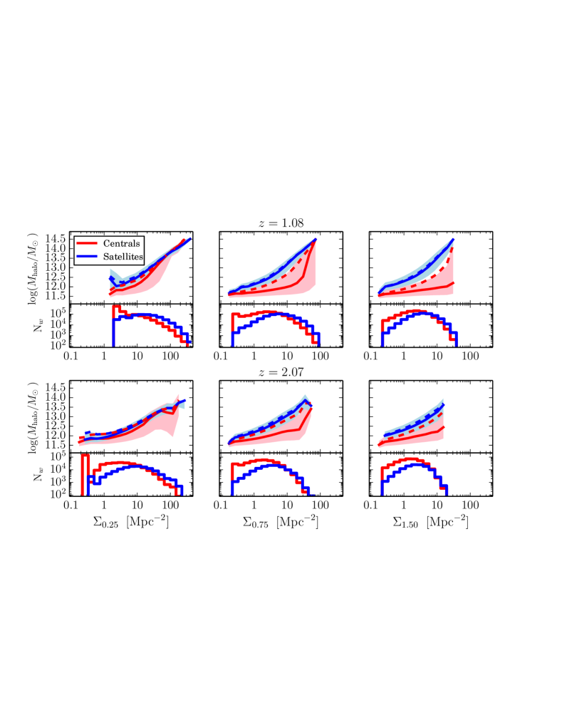
Figure 2: Median mass of the parent halo of each galaxy as a function of density measured on three scales $\Sigma_{0.25}$ (left panels), $\Sigma_{0.75}$ (central panels), and $\Sigma_{1.50}$ (right panels) for central galaxies (red solid lines) and satellites (blue solid lines) at $z=1.08$ (top panels), and $z=2.07$ (bottom panels). The shaded areas are bounded by the 25th and 75th percentiles of the distributions. Dashed lines correspond to the mass of the most massive halo within 1 Mpc ($M_{\rm{h,1Mpc}}$, see text). The distribution of densities for centrals and satellites are shown in the lower part of each panel.

In this section we examine correlations of density measured on different scales with halo mass for both central and satellite galaxies at $z=1.08$ and $z=2.07$. This compliments recent work in the local Universe by Muldrew et al. (2012), Haas et al. (2012), and Hirschmann et al. (2014).

Figure 2 shows the correlation of median (and 25^th and 75^th percentile) halo mass with density on three scales: $\Sigma_{0.25}$ (left panels), $\Sigma_{0.75}$ (central panels), and $\Sigma_{1.50}$ (right panels) for central galaxies (red solid lines) and satellites (blue solid lines). In each panel, the histograms at bottom show the weighted distribution of density for centrals and satellites on the same scales . The top and bottom rows refer to $z=1.08$ and $z=2.07$, respectively. The binning is logarithmic in density and galaxies with no neighbours within the aperture ($\Sigma_{r_{o}}=0$) are included in the first bin that is populated with objects at each scale. From a first look at the distributions it is clear that the three different scales probe different ranges of density. The bigger the aperture the lower is the density that can be measured.

For satellite galaxies the correlation is remarkably good at all scales and all redshift: in this redshift range even the smallest aperture we use (0.25 Mpc) is big enough to recover a density dependence for the satellites.

The halo mass dependence on density for centrals is a strong function of the aperture size. The typical virial radius of a $10^{13}M_{\odot}$ (resp. $10^{14}M_{\odot}$) halo is 0.30 (resp. 0.63) Mpc. As a result the 0.25 Mpc aperture probes intra-halo scales for all reasonably massive haloes, and a good correlation with density (which is almost indistinguishable from that of satellites) arises. Despite the low number counts in this small aperture, the correlation we find is not unexpected. It follows from a power law dependence of median halo mass on group size (defined as the number of galaxies above the stellar mass limit which live in the same dark matter halo). This correlation extends to small group sizes ($2-3$ members per group) and holds for centrals as well as for satellites. This happens whenever the aperture size does not extend well beyond the halo virial radius. Taking a look at the distribution of density on 0.25 Mpc scale it is clear that, while a population of isolated centrals exists at ($\Sigma_{0.25}<5{\rm Mpc^{-2}}$), the higher densities are also well populated by central galaxies It is indeed at those high densities that we find a good correlation with the group size.

Looking at the 25^th and 75^th percentiles of the halo mass distribution at fixed density (shaded region in Figure 2) we notice that the trend is much tighter (smaller scatter) for satellite galaxies than for centrals. Indeed the 75^th percentile for centrals tracks, albeit with some changes, the halo mass of satellites at fixed density on all scales, while the median and to a greater extent the 25^th percentile drops to much lower halo mass as the scale and density increases (almost erasing any correlation with halo mass). In other words: there exists a significant population of central galaxies at high density which inhabit low mass haloes, and the size and relevance of this population increases to larger scales.

We quantify this statement in Figure 3 which shows the halo mass distributions in a fixed bin of density (15-20 Mpc^-2) on scales 0.25 Mpc (top panel), 0.75 Mpc (middle panel), and 1.50 Mpc (bottom panel) at $z=1.08$. This bin is chosen to probe a fairly high density with good statistics on the three scales although it is a more unusually large density when measured on larger scales. Satellites at this density occupy a peak of relatively high halo mass, demonstrating the tight correlation between halo mass and density seen in Figure 2. A significant fraction of central galaxies live in the same peak, illustrating the relative insensitivity of a “density within an aperture” statistic to whether a galaxy is the central or a satellite galaxy of a massive halo. However there is also a second significant population of central galaxies at low halo mass: 52% (61%, 65%). These galaxies live in small haloes (which is why they are usually centrals) but have a high number of neighbouring galaxies which live within the cylindrical aperture used to measure density – a number which can only increase with the aperture size. This phenomenon is important when a significant fraction of the neighbouring galaxies used to trace density live outside the galaxy’s own host halo – i.e. when the aperture scale is larger than the virial radius of the halo. This explains why the scatter becomes small when densities are measured on a 0.25 Mpc scale, while on the 0.75 Mpc scale (at $z=1.08$) the median shoots up at the very highest densities – such densities are most often obtained at the centres of massive haloes which have virial radii close to 0.75 Mpc. However, in all other regimes, the low halo mass population is the dominant one for central galaxies at intermediate to high density.

Our goal is to calibrate the environment of galaxies using measurements of density: Figure 3 shows that this is a degenerate problem where we have only a single measurement of density within an aperture. In Appendix A we examine how the combination of two scales can break this degeneracy, while in Section 6 we ignore the second peak by excluding low (stellar) mass galaxies at high density. Trends driven by the population of low halo (or stellar) mass centrals at high density are difficult to interpret because they can have actual physical association with the nearby massive halo to which they have (at the current snapshot) not been assigned. Using an N-body simulation and accurately tracing the trajectories of ejected satellites, Wetzel et al. (2013) have shown that infalling galaxies can pass through a massive halo on radial orbits and emerge out the other side, where they extend out to 2.5 times the virial radius of the halo they crossed. They compose 40% of all central galaxies out to this radius and their evolution is likely to have been influenced by satellite-specific processes. This “backsplash” population has also been investigated by Mamon et al. (2004); Balogh et al. (2000); Ludlow et al. (2009) and Bahé et al. (2013), as well as Hirschmann et al. (2014) who also find that such additional processing of low mass, high density galaxies is necessary to explain the density dependence of the passive fraction of central galaxies at low redshift. Thus an accurate accounting for this population is essential.

To examine the actual real-space proximity of galaxies to massive haloes, we consider the most massive halo within a sphere of 1 Mpc ($M_{\rm{h,1Mpc}}$). In Figure 3 we show the distribution of $M_{\rm{h,1Mpc}}$ (black, dashed line). This does not completely exclude the low halo mass population, but reduces it substantially. The fraction of centrals with $M_{\rm{h,1Mpc}}<10^{12.5}M_{\odot}$ is 37% (32%, 30%), far fewer than where the host halo mass is used. Most remaining such galaxies are in this high-density bin due to redshift space projection. However this tells us that almost half of low halo mass central galaxies at this density are within 1 Mpc of a massive halo and many may have already passed through that halo. Thus for a clean selection of central galaxies which have not suffered such effects, it seems sensible to exclude those at high density. In Figure 2 we overplot the median relation of density with $M_{\rm{h,1Mpc}}$ (dashed line). The reduced peak at low mass means that this more closely follows the 75^th percentile of halo mass, and approaches that of satellites (for which the low halo mass peak is negligible).

In order to test the effect of redshift accuracy, we repeat the analysis on the lowres-z sample. Our results show that none of the trends presented in this section notably change, the main effect being a smoothing of the highest density peaks, slightly reducing the median halo mass. Conversely, when photometric redshifts are used we notice two effects. First, the median halo mass at fixed density is reduced both for centrals and satellites on all scales. The 0.75 and 1.50 Mpc scales are the most affected. The median halo mass for centrals is constant with density at $10^{12}M_{\odot}$. For satellites this is 0.5 dex higher and increases with density only at $\Sigma>10{\rm Mpc^{-2}}$. On the 0.25 Mpc scale a good correlation of median halo mass with density still exists, but with a larger scatter both for centrals and satellites. The second effect we find is in the distributions of density, which are narrower than in the hires-z case, reducing the density dynamic range. In Figure 4 we compare the density in the hires-z sample to those in the photo-z sample for the 0.75 Mpc aperture. The black dashed line marks the 1:1 relation. We show two velocity cuts for the photo-z sample: $dv=1500km/s$ (red) and $dv=7000km/s$ (blue). In the upper panel the distribution of densities is plotted for the hires-z sample and in the right panel we show the density distributions for the two apertures used for the photo-z sample. Both from the contours and the histograms it is evident that $dv=1500km/s$ misses many objects in the most dense regions, while with a larger depth $dv=7000km/s$ we re-incorporate those galaxies obtaining a good correlation with the hires-z measurements. Moreover, using photo-z, the low densities are devoid of galaxies which end up at intermediate densities. Also this effect is less severe for the 0.25 Mpc aperture. Thanks to the large statistics, we can probe a wide range of density in the models, however this is reduced when considering the number of objects in a real survey.

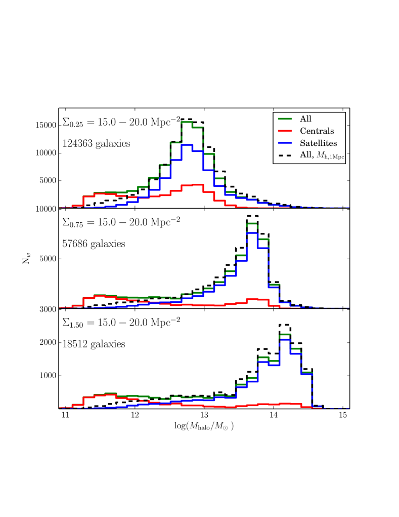
Figure 3: Weighted distributions of parent halo mass for each galaxy in a fixed bin of density (15-20 Mpc^-2) on scales $\Sigma_{0.25}$ (top panel), $\Sigma_{0.75}$ (middle panel), and $\Sigma_{1.50}$ (bottom panel) at $z=1.08$. The dashed line shows the weighted distribution of the most massive halo mass within 1 Mpc of each galaxy (see text).

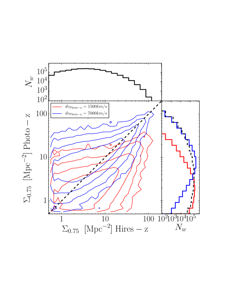
Figure 4: Main panel: Density on the 0.75 Mpc scale for the photo-z sample and different velocity cuts ($dv=1500km/s$ red and $dv=7000km/s$ blue) as a function of density in the same aperture (and $dv=1500km/s$) for the hires-z sample. The contours are logarithmically spaced with the outermost contours at 25 objects per bin and the innermost at $10^{4}$ objects per bin. Upper panel: weighted distribution of density for the hires-z sample. Right panel: weighted distributions of density for the photo-z sample with the same velocity cuts as above. The distribution of density for the hires-z sample (dashed black) is repeated here for comparison.

Finally we test if the distributions shown in figure 3 would change at the low halo-mass end due to the resolution of the N-body simulation. The history of galaxies whose parent haloes are below $10^{12}M_{\odot}$ cannot be traced accurately along the halo merger trees, thus their physical properties might be inaccurate. We perform the same exercise using the G13 model applied to the Millennium-II simulation scaled to WMAP7 parameters following Angulo & White (2010). This simulation has a smaller cosmological volume but a particle resolution about 100 times better. The distribution of halo masses for centrals and satellites below $10^{12}M_{\odot}$ is unchanged, probably thanks to our conservative limit in stellar mass.

5 Mass rank as a method to disentangle centrals and satellites

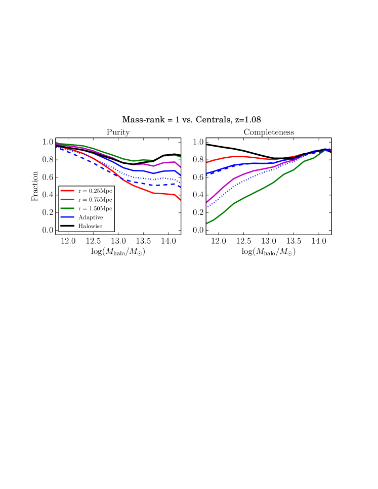
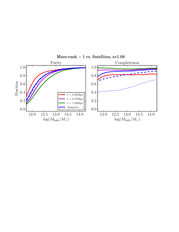
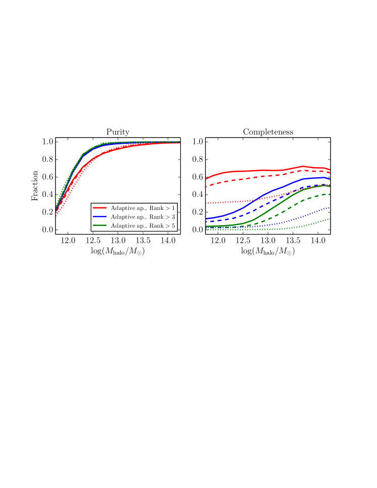
Figure 5: Top panels: purity and completeness for the selection of central galaxies based on stellar mass rank = 1 as a function of the halo mass. The rank is computed in various apertures ranging from 0.25 to 1.50 Mpc for the $z=1.08$ bin. Solid lines refer to the hires-z, dashed lines to the lowres-z and dotted lines to the photo-z samples. Middle panels: same as before but for satellite galaxies selected by having stellar mass rank $>1$. Bottom panels: comparison between different rank criteria for the selection of satellite galaxies using the adaptive aperture.

It is also critical to describe whether a galaxy dominates its halo (and the local gravitational field) or if it is instead orbiting within a deeper potential well. This can be modelled (and is in SAMs) assuming a dichotomy between central and satellite galaxies. Central galaxies accrete gas by cooling, and merge with their satellites. In contrast, satellite galaxies orbit within the gravitational field, and move with respect to the intra-halo gas, thus experiencing tidal interaction and stripping effects. This has been both directly observed in nearby clusters (see e.g. Boselli et al., 2008; Yagi et al., 2010; Fossati et al., 2012) and indirectly witnessed from statistical studies (Balogh et al., 2004). Moreover, it has been claimed that, while the properties of galaxies are shaped by intrinsic parameters, (e.g. stellar mass Peng et al. 2010; Kovač et al. 2013, see however De Lucia et al. 2012), satellites’ properties are also influenced by their environment (Peng et al., 2012; Woo et al., 2013). A reliable method to separate centrals from satellites in observations is therefore crucial.

5.1 Identification of central galaxies

Central galaxies are usually the most massive galaxy in their halo (but not always, see Skibba et al. 2011). This follows from the fact that the other – satellite – galaxies in the halo were formed at the centre of less massive progenitor haloes. Therefore a sample of central galaxies can be identified by assuming that the most massive galaxy in a halo is also its central galaxy (e.g. Yang et al., 2008).

We compute the rank in stellar mass of each galaxy in several circular apertures. We examine both fixed radius apertures, and a radius that depends on stellar mass (accessible from observations). This approach resembles the Counts-in-Cylinders method (Reid & Spergel 2009, see also Trinh et al. 2013). However, it is worth stressing that previous applications of this method were focused on different science goals (e.g. the identification of 2 member groups in a specific survey). We present here a detailed analysis of how much a population of galaxies whose stellar mass rank is 1 compares to galaxies identified as centrals by the algorithms used in the models (see sec. 2).

We define two parameters to quantify the overlap between the two populations. The purity ($P$) is the number of centrals which are correctly identified over the number of selected galaxies; and the completeness ($C$) is the number of identified centrals over the total number of central galaxies.

In this section (and in Sections 5.2 and 5.3) the use of the weights for each galaxy has a negligible impact on both the qualitative and the quantitative results. The method is insensitive to the overestimation of the number of low mass galaxies because the galaxies which compete to be the most massive in an aperture have similar stellar masses, thus the same weight. Therefore we do not use the weights in this Section.

In the top panels of Figure 5 the purity and the completeness of identified centrals are plotted as a function of halo mass. Solid coloured lines correspond different apertures for the hires-z sample ranging from 0.25 Mpc to 1.5 Mpc. Ideally one would like to maximise both $P$ and $C$ but a trade-off must be found. In table 1 the performances of different methods are given. Purity and completeness are given for haloes above and below $10^{13}M_{\odot}$ and for the complete sample.

We start by identifying the “halo-wise” mass rank of each galaxy by ranking in stellar mass all the galaxies belonging to the same halo. We obtain the black solid line in the top panels of figure 5. The purity and completeness of this sample describes the ideal overlap between mass rank 1 and central galaxies. The completeness is limited by the fact that the most massive galaxy is not always the central of its host halo. This is true especially at halo masses around $10^{13}M_{\odot}$ where this incompleteness reaches 20%. Due to the scatter in the stellar-mass halo-mass relation for central galaxies, haloes of masses $\sim 10^{12-13}M_{\odot}$ can all host galaxies of equivalent stellar mass which means that even in minor halo mergers (down to a mass ratio of $\sim 1:10$) a more massive galaxy can be supplied by the less massive halo. It will then become a satellite more massive than the central of the final halo. The purity and completeness estimates are always computed relative to the population of “true” central galaxies in the model – as such the halo-wise values provide an upper limit on completeness, and an“optimal” purity based on the assumption that we perfectly know the content of each halo. However the most massive galaxy in any halo corresponds to a significant local potential, and as such one could also define a purity and completeness relative to this population. Such estimates of purity and completeness would clearly be significantly higher than those defined here (relative to the central population).

Looking at Figure 5, it is clear that fixed apertures (red, magenta, and green solid lines) struggle to balance the requirements for both high purity and completeness. The general trend is for an increasing purity and decreasing completeness as the aperture size is increased. However, for small apertures (0.25 Mpc) $P$ goes down at the high halo mass end because the aperture covers only a fraction of the halo; if they are too large then $C$ goes down in smaller haloes because one aperture covers multiple haloes.

From this evidence and based on the idea that a good correlation exists between stellar mass and halo virial radius (which is an analytic function of halo mass) for centrals, we define an “adaptive” aperture as follows:

$$r=\rm{min}(0.75,n\times 10^{(\alpha\log M_{*}+\beta)})~{}\rm{[Mpc]}$$ (3)

where $M_{*}$ is the stellar mass of the galaxy, $n$ is a multiplicative factor, and $\alpha$ and $\beta$ are the parameters which describe the dependence of virial radius on stellar mass for centrals in the models . From the models we get $\alpha=0.25$, $\beta=-3.40$ at all redshifts and after extensive testing we define $n=3$ in order to avoid very small apertures that would decrease the purity. In order to limit the size of the aperture to a scale that entirely covers the most massive haloes without extending beyond, we limit the aperture to a radius of 0.75 Mpc. From Figure 5 and from the values in table 1 it is evident that this is a great improvement for $C$ at low halo masses relative to the fixed 0.75 Mpc aperture, while we lose 8% in purity at high halo masses. This is because we are using a small aperture for low mass galaxies (0.2 Mpc for $M_{*}=10^{9.5}M_{\odot}$). Since some of them are satellites living in massive haloes, the apertures we use are too small to encompass the entire halo and those satellites can get high mass rankings reducing $P$.

	$\log M_{\rm h}\leq 13$		$\log M_{\rm h}>13$		All
Aperture	$P$	$C$	$P$	$C$	$P$	$C$
	$z=1.08$
0.25 Mpc	0.92	0.82	0.52	0.87	0.88	0.82
0.75 Mpc	0.94	0.40	0.75	0.78	0.92	0.42
1.50 Mpc	0.94	0.17	0.80	0.64	0.91	0.19
Adaptive	0.94	0.68	0.75	0.78	0.92	0.69
	$z=2.07$
0.25 Mpc	0.93	0.79	0.76	0.91	0.92	0.79
0.75 Mpc	0.95	0.38	0.86	0.83	0.94	0.40
1.50 Mpc	0.95	0.18	0.88	0.71	0.94	0.20
Adaptive	0.94	0.64	0.84	0.86	0.94	0.65

Table 1: Purity and completeness for the identification of central galaxies using stellar mass rank = 1 in four different apertures for haloes below and above $M_{\rm halo}=10^{13}M_{\odot}$, and for the full hires-z sample at $z=1.08$ and $z=2.07$.

5.2 Identification of satellite galaxies

	$\log M_{\rm h}\leq 13$		$\log M_{\rm h}>13$		All
Aperture	$P$	$C$	$P$	$C$	$P$	$C$
	$z=1.08$
0.25 Mpc	0.58	0.78	0.97	0.79	0.70	0.78
0.75 Mpc	0.33	0.92	0.96	0.93	0.45	0.93
1.50 Mpc	0.27	0.97	0.91	0.96	0.38	0.96
Adaptive	0.46	0.86	0.95	0.91	0.59	0.88
	$z=2.07$
0.25 Mpc	0.49	0.79	0.93	0.83	0.56	0.80
0.75 Mpc	0.28	0.92	0.90	0.92	0.33	0.93
1.50 Mpc	0.24	0.96	0.85	0.94	0.29	0.95
Adaptive	0.37	0.84	0.92	0.91	0.44	0.84

Table 2: Purity and completeness for the identification of satellite galaxies using stellar mass rank $>1$ in four different apertures for haloes below and above $M_{\rm halo}=10^{13}M_{\odot}$, and for the full hires-z sample at $z=1.08$ and $z=2.07$.

The mass rank method can also be used to identify satellite galaxies, under the assumption that satellites are less massive than the central galaxy of their own halo, i.e. mass rank $>1$. In the middle panels of Figure 5 are plotted the purity and completeness (defined as in Section 5.1) of our identified satellite galaxies as a function of halo mass. The purity is limited - but only by  5% - by satellites that are more massive than the central galaxy of their host halo. The purity quickly drops at halo masses below $10^{12.5}M_{\odot}$, with little dependence on the aperture size. In Table 2 we present the values of $P$ and $C$ for satellite galaxies living in haloes less and more massive than $10^{13}M_{\odot}$, and for the complete sample. It is clear that the overlap between mass rank $>1$ and satellites is strong among massive haloes, while in less massive haloes about half of the galaxies with mass rank $>1$ are centrals which by chance have one (or more) more massive neighbours within the aperture but not within the same halo. It is hard to define a satellite in this halo mass regime, especially where the stellar mass of central galaxies approaches the mass limit: the mass of any satellites included in the sample must therefore be close to that of their central. This halo mass regime consists primarily of isolated galaxies and loose proto-groups (namely pairs or triplets). Completeness in contrast is remarkably high over the full range of halo masses, illustrating that our method is effective in picking up a complete population of satellites.

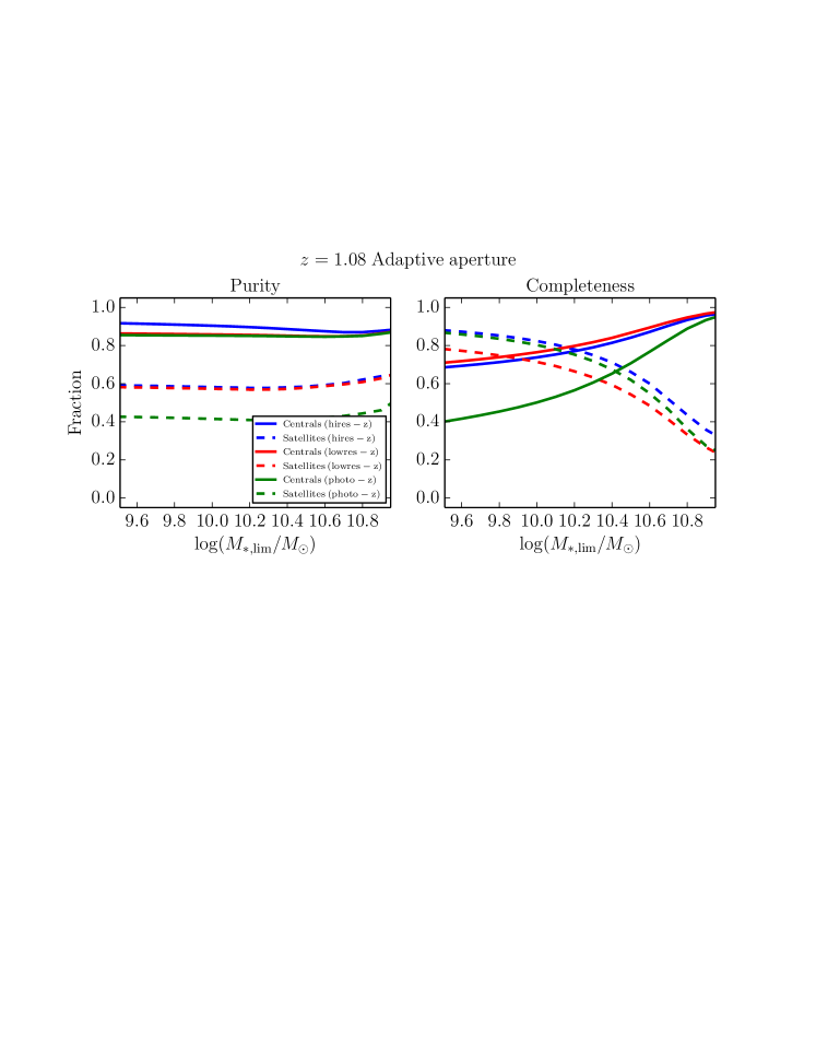
Figure 6: Purity and completeness for the identification of central (solid lines) and satellite (dashed lines) galaxies using stellar mass rank = 1 ($>1$) in the adaptive aperture at $z=1.08$ for the hires-z sample (blue lines), for the lowres-z sample (red lines) and for the photo-z sample (green lines).

In the bottom panels of Figure 5 we explore the dependence of $P$ and $C$ on the stellar mass rank we required to identify a satellite within the adaptive aperture. Setting two more conservative limits (rank $>3$ blue solid and $>5$ green solid) we achieve a small improvement in the purity at low halo masses but with a dramatic degradation of the completeness. It is clear that with rank to be $>5$ ($>3$) we are implicitly selecting only galaxies that have at least five (three) companions within the aperture, all of them more massive. Moreover, especially at low/intermediate halo masses, the number of galaxies within a halo is often smaller than five (three). Thus many real satellites are missed.

Based all this evidence our preferred method to identify central (satellite) galaxies is to require a stellar mass rank $=1$ ($>1$) in the adaptive aperture. The purity and completeness values for this aperture are $P=0.93$ and $C=0.67$ for centrals and $P=0.60$ $C=0.90$ for satellites in the hires-z sample at $z=1.08$. The use of the same aperture for both types has the advantage of making the two selections mutually exclusive. If two different apertures are used for selecting centrals and satellites, the fraction of interlopers has to be taken into account as one galaxy might be the most massive in one aperture but not in the other one. Finally it is worth stressing that both the purity and the completeness of the full samples of centrals and satellites are completely independent of the measured density and any effort to calibrate halo mass. The key parameters are the scale over which the rank is computed and the assumption that central galaxies are typically more massive than nearby satellites. This assumption holds well in the G13 models and is typically assumed to be true in group reconstruction using observational data (e.g. Yang et al., 2007).

5.3 Dependence of Purity and Completeness on the stellar mass selection limit

To avoid model resolution biases in our definition of the environment, we probe down to a constant mass limit of $M_{*}=10^{9.5}M_{\odot}$. This is deeper than most observational surveys at these redshifts. To examine more realistic survey depths, we now test how our selection methods perform as a function of the stellar mass limit $M_{*,\rm{lim}}$. In Figure 6 we show $P$ and $C$ for the identification of both centrals and satellites as a function of $M_{*,\rm{lim}}$ using the adaptive aperture. The purity is almost unaffected by the selection limit while, as expected, completeness is. Regarding the centrals, the overall purity is about $90\%$ and does not depend on the aperture nor on the mass limit. Conversely $C$ is a strong function of the minimum stellar mass. When low mass galaxies are removed, the sample of centrals with mass rank 1 becomes more and more complete. The completeness never reaches unity because, as discussed before, there are satellites which are more massive than the centrals of their own haloes.

As already discussed, the purity for the satellites is about 60% for all stellar mass limits. This happens because, close to the stellar mass limit and within 0.75 Mpc, two-halo pairs containing similar mass centrals are just as common as pairs of similar mass galaxies within one halo. For this reason there is an improvement using the adaptive aperture as it is smaller than 0.75 Mpc at low stellar masses and this helps in limiting the contamination from centrals. The completeness shows a well defined decreasing trend at increasing mass limits because the higher $M_{*,\rm{lim}}$, the higher the chance that a satellite is more massive than the central of its halo. This, combined with the low number of massive satellites, makes the fraction drop below 40% at $M_{*,\rm{lim}}>10^{10.8}M_{\odot}$.

These results stand even when the stellar masses are convolved with a gaussian random error to mimic observational uncertainties. We tested the effect of errors up to a relatively large value of 0.5dex. The purity for centrals and the completeness in the identification of satellites decrease by less than 5%, while the purity for satellites and the completeness of centrals decrease by 10%. Moreover, the trends as a function of the mass uncertainty are smooth and the values given here are to be considered upper limits.

5.4 Dependence on Redshift Accuracy

The trends discussed so far have been drawn using the hires-z sample. In this section we analyse how they change using less accurate redshifts. Dashed lines in Figure 5 are for the lowres-z sample and dotted lines are for the photo-z sample using only the adaptive aperture. The general trends apply to the fixed apertures as well.

Concerning central galaxies, the purity is decreased by $\sim 10-15\%$, due to the smoothing of the density field introduced by lowres-z and photo-z. This happens because massive centrals are projected outside the cylinder of less massive satellites (the latters then scoring a mass rank 1, thus reducing the purity of the selection ). The completeness on the other hand is not affected in the lowres-z sample because massive centrals are still identified as the most massive galaxies in their cylinders. The larger velocity cut we use for the photo-z sample has a positive effect on the purity but decreases the completeness. This is not unexpected because the larger velocity cut increases the volume of the cylinder where we compute the mass rank, therefore the final effect is similar to increasing the size of the aperture.

In the case of satellites the purity is not affected by the smoothing in the redshift direction because the population of rank $>1$ galaxies is still mainly composed of satellites. Conversely the completeness is decreased by $\sim 10\%$, and $\sim 40\%$ for the lowres-z and photo-z respectively. As photo-z are much less accurate than spectroscopic redshifts it is worth noting why the performance of the method is still reasonably good. When the mass rank based method identifies a galaxy as a satellite, it does not mean we know it to be a satellite of a specific halo. Therefore the use of photo-z can project both the “true” central and one (or more) satellites outside their original halo. When this happens, the central/satellite status is preserved and a satellite galaxy is now identified as central in the original halo. If, as it is more likely, only satellites are projected outside the halo, the most massive is identified as a central, thus reducing the satellites’ completeness.

When the less accurate redshifts are used, we find no major impact on the trends of $P$ and $C$ on the stellar mass limit. The strongest effect is found on the completeness of the identification of satellites which follows the same trend described above.

5.4.1 Dependence of Purity and Completeness on the spectroscopic sampling rate

Here we examine the performances of our method in the case of variable sampling rate. Our approach is to progressively reduce the spectroscopic sampling rate from $100\%$ to $0$ in steps of $10\%$ by randomly replacing the hires-z (or lowres-z) with photo-z. Figure 7 shows the purity and completeness in the adaptive aperture at each sampling rate. The main conclusions have been discussed above using pure spectroscopic (hi- and low-res) redshifts and photo-z. Here we only note that the decline in purity is roughly linear as a function of the sampling rate for both centrals and satellites and that the completeness for satellites decreases more significantly from full sampling rate to $50\%$ rather than from this value to pure photo-z.

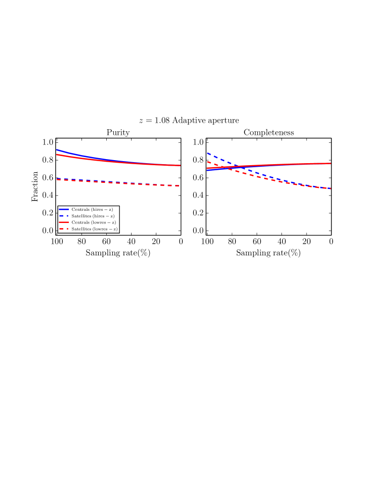
Figure 7: Purity and completeness for the identification of central (solid lines) and satellite (dashed lines) galaxies using stellar mass rank = 1 ($>1$) in the adaptive aperture for incomplete hires-z (blue lines) and lowres-z (red lines) sampling at $z=1.08$.

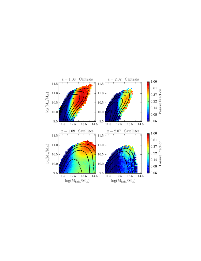
Figure 8: Fraction of passive galaxies (as defined in Section 2.1) as a function of halo mass and stellar mass for centrals (top panels) and satellites (bottom panels). Redshift increases from $z=1.08$ (left panels) to $z=2.07$ (right panels). The contours are drawn from the density of galaxies in the parameters space and are log-spaced with the outermost contour at 25 objects per bin and the innermost at $10^{4}$ objects for centrals and $10^{3.4}$ for satellites.

Several other works have attempted a selection of central and satellite galaxies in real spectroscopic surveys. Among them Knobel et al. (2012) used a probability based method to assign a binary central/satellite classification to the I-band flux limited sample in the zCOSMOS survey. The spectroscopic sampling rate is about $50\%$ in the redshift range $0.1-0.8$. Despite the different identification method and the broad redshift range (which hampers the definition of a fixed stellar mass limit), their final results ($P=0.81~{}C=0.89$ and $P=0.62~{}C=0.45$ for centrals and satellites respectively) agree with our results at the same sampling rate within $\sim 5\%$ for the purity and $\sim 15\%$ for the completeness.

In conclusion, it is remarkable how the purity and the completeness both centrals and satellites are not strongly affected by low spectroscopic sampling rates nor by the survey detection threshold, this proving the robustness of the method and its usefulness in surveys with different designs.

6 Relation between environment and passive fraction

In this section, we examine if and how well the environmental trends predicted by the models can be recovered using quantities accessible from observations, e.g. density and mass rank. We focus our attention on a single physical quantity: the fraction of passive galaxies. Peng et al. (2010, 2012) and Woo et al. (2013) have shown that the passive fraction of satellite galaxies correlates strongly with a measurement of local density, labelled “environment”, while for centrals it is a function of their stellar mass (Peng et al., 2010, 2012) and halo mass (Woo et al., 2013).

6.1 The growth of a passive population in the models

First of all we investigate how the fraction of passive galaxies depends on stellar mass, halo mass and central/satellite status. The former basically describes the integrated star formation and merger history of a galaxy, while the latter two are strongly correlated to the regulation of its star formation in the models. Figure 8 shows the passive fraction in the $M_{*}-M_{\rm halo}$ space for centrals (top panels) and satellites (bottom panels), at redshifts 1.08 (left) and 2.07 (right). The contours are drawn from the density of galaxies in the parameters space and are logarithmically spaced with the outermost contour at 25 objects per bin and the innermost at $10^{4}$ objects for centrals and $10^{3.4}$ for satellites. Each bin has to contain at least 10 objects for the passive fraction to be computed, and the color coding is scaled logarithmically.

A common feature across the redshift bins is that centrals and satellites populate different regions of the parameters space. The centrals populate a sequence where the stellar mass linearly increases with halo mass (in log-log space). In contrast the satellites form a cloud that spans all halo masses such that $M_{\rm halo}^{\rm sat}(M_{*})\geq M_{\rm halo}^{\rm cen}(M_{*})$.

At halo masses above $10^{12.5}M_{\odot}$ a passive population of centrals starts to appear at $z\sim 2$, becoming dominant as the redshift decreases to 1. Those passive centrals move to higher halo masses without increasing their stellar mass enough to stay on the relation defined by the star forming centrals. The passive fraction increases to about $80\%$ for centrals in haloes more massive than $10^{13}M_{\odot}$. Wilman et al. (2013), using Wang et al. (2008) models (an early version of G13) at $z=0$, showed that a strong correlation between bulge growth and passive fraction exists for massive centrals in SAMs. The physical reason is that for those galaxies the cold gas reservoir is exhausted by a merger induced starburst and further cooling of the gas is prevented by the strong radio-mode AGN feedback. Although these trends do not perfectly reflect the observed data, they are qualitatively similar to those shown by Kimm et al. (2009) at $z=0$ for different published SAMs. In their work the model by De Lucia & Blaizot (2007, another early version of G13) appears to be the closest to the observational constraints.

Also the passive fraction of satellite galaxies shows significant evolution. As time goes by (and redshift decreases) the satellite cloud extends to higher halo masses, and a population of passive satellites appears at high stellar masses. Most of the passive satellites are likely to be turned passive by the stripping mechanisms acting in massive haloes. However, the highest passive fractions are found at both high halo mass and stellar mass. These galaxies were probably already passive when they were centrals and then merged with a more massive halo becoming passive satellites.

6.2 Recovering predicted trends with observational proxies

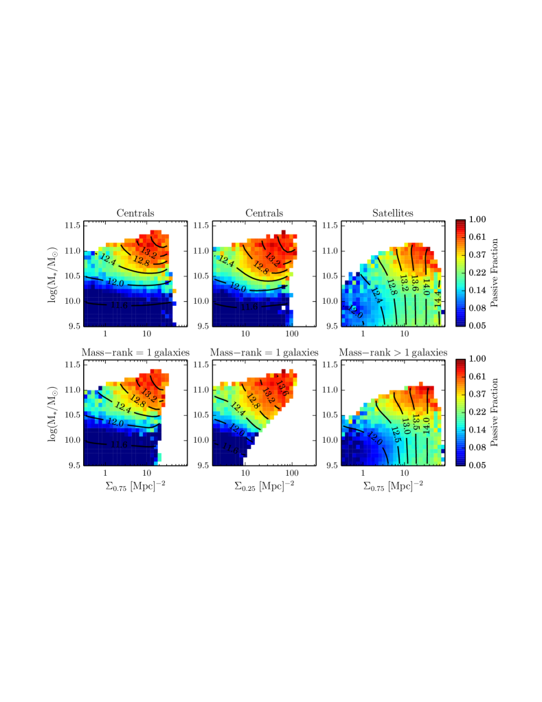
Figure 9: Fraction of passive galaxies as a function of density on the scale $\Sigma_{0.75}$ and stellar mass for central galaxies (left panels), on the scale $\Sigma_{0.25}$ for centrals (central panels) and on the scale $\Sigma_{0.75}$ for satellite galaxies (right panels), at $z=1.08$. The central/satellite definition is the one provided by the SAMs in the top panels and the one defined by the mass rank in the adaptive aperture in the bottom panels. The contours are drawn from the median halo mass in the same bins.

In this section we investigate if, and how well, the predicted trends of passive fraction as a function of halo mass and stellar mass can be recovered using only observable quantities. We make use of the density of galaxies in fixed apertures and the choice of centrals and satellites is performed both using the model definition and the observational mass rank method presented in Section 5. We recall that the densities, number density contours and the median halo mass values presented in this section are obtained after application of the statistical weights described in Sections 2.1, and 3.

In Figure 9 we show the fraction of passive galaxies (at $z=1.08$) as a function of density and stellar mass for centrals (left and middle panels) and satellites (right panels). The top row makes use of the separation between these two types as coded in the models, while the bottom row uses the mass rank in the adaptive aperture in order to divide the two types. The contours describe the median halo mass in the same bins of stellar mass and density. Again, each bin has to contain at least 10 objects for the passive fraction to be computed. A close examination of the direction of change for passive fraction relative to both the axes and to the direction of change for median halo mass, allows us to evaluate how well we can use the parameters to track the trends seen in the pure model space (see Figure 8).

Let us start with the centrals. We know from Figure 8 that the passive fraction increases primarily with halo mass, and that at fixed halo mass there is if anything a slight anti-correlation with stellar mass. Can we see this in the observational parameter space?

In the left panels in Figure 9 the density has been computed on scales of 0.75 Mpc, which covers a super-halo scale for all the haloes of mass below $10^{14}M_{\odot}$. To examine mostly intra-halo scales, we also examine the density computed on the smallest scale (0.25 Mpc, middle panels).

From the top panels, and without the halo mass contours, it would appear that the stellar mass is the main driver of the correlation with passive fraction. Indeed this confusion is caused by the wide range of density seen at low stellar mass: densities are reached which are just as large as those for the centrals of high mass haloes (even on 0.25 Mpc scales). as discussed in Section 4. However, when the halo mass contours are compared to the direction of increase of the passive fraction, it is evident that the halo mass is the main driver of the trend.

In the models, the low mass galaxies at high density show a passive fraction that is very similar to those at low density and comparable mass. However in the real Universe those galaxies may have already experienced physical processes driven by massive haloes, even if they are currently outside the virial radius – i.e. the “backsplash” population discussed by Mamon et al. (2004); Balogh et al. (2000); Ludlow et al. (2009); Bahé et al. (2013); Wetzel et al. (2013); Hirschmann et al. (2014). Indeed, observational data suggests they behave more like satellites (Wetzel et al., 2013; Hirschmann et al., 2014). This implies that when the method is applied to an observational dataset, it is useful to “clean” the sample of these high density, low mass objects. Fortunately, this happens as a direct consequence of making a mass rank 1 selection as in the bottom panels. The adoption of the adaptive aperture means that our mass rank 1 galaxies are the most massive within an aperture not larger than 0.75 Mpc but not smaller than 0.28 Mpc for galaxies in our stellar mass range. Galaxies at low mass and high 0.25 Mpc density are inevitably not the most massive within this aperture, and are excluded. However this correlation depends on both density and stellar mass because the halo mass for central galaxies depends on both these parameters.

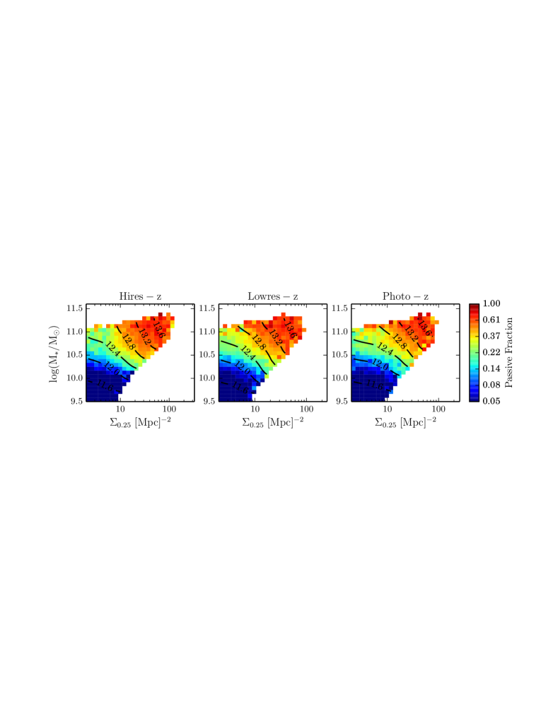
Figure 10: Fraction of passive galaxies as a function of density on the scale $\Sigma_{0.25}$ and stellar mass for mass rank 1 galaxies (in the adaptive aperture) using hires-z (left panel), lowres-z (central panel), and photo-z (right panel) at $z=1.08$. The contours are drawn from the median halo mass in the same bins.

For satellites (which dominate in mass and number within the rich haloes), the correlation between halo mass and density is very good irrespective of the aperture used (the contours in the right panels of Figure 9 are essentially vertical). Therefore the passive fraction trends as a function of halo mass and stellar mass are easy to qualitatively recover using the density and either the satellite definition in the SAMs or the one coming from the mass rank. The low mass - high density central population removed by the mass rank method ends up in the cloud of satellites. While those galaxies dominate the low mass centrals at high density, they do not contribute much to the satellites at the same stellar mass and density. Density computed on either 0.25 or 0.75 Mpc work well in this regard.

A general conclusion is that a well calibrated halo mass dependence on the observed properties (stellar mass, density) is crucial in understanding which physical properties are shaping the trends (in this case the passive fraction) we observe. While the results can be already be achieved with the SAM definition of centrals and satellites, it is important to stress that the use of the observationally motivated mass rank method provides the same result.

Finally, Figure 10 shows how the passive fraction trends change if less accurate redshifts are used, as in our lowres-z and photo-z samples. We restrict ourselves to central galaxies defined with the mass rank method in the adaptive aperture and density computed on the 0.25 Mpc scale. Decreasing the quality of the redshift survey, the density - stellar mass correlation is less tight and the number of galaxies at the highest densities is reduced. The conclusions that can be drawn in this parameter space are unchanged. However, we stress that this conclusion comes with a number of caveats. First, the density dynamic range is reduced when photo-z are used on all scales, but less so for 0.25 Mpc. This small scale can only be used if the galaxy sampling is good enough, e.g. the stellar mass limit is low as in this work. Second, the use of the mass rank method “cleans” the sample of low mass centrals which are projected in high density regions due to the less accurate photo-z, allowing us to obtain a trend similar to that for hires-z. Moreover, the density field is well reconstructed only with very good photometric redshifts. The photo-z accuracy typically depends on the number of photometric data points and their distribution across the rest-frame galaxy spectral energy distribution, generally being worse for fainter objects. Therefore, we warn the reader that the performance of photo-z in recovering the true density field should be carefully assessed for each individual sample, along with the significance of any particular result based on this approach.

7 Conclusions

In this work we have characterised the definition of “galaxy environment” by means of the projected density within fixed apertures at $z\sim$ 1-2. We have tested our methods by applying them to the semi analytic models of galaxy formation presented by Guo et al. (2013) and based on a new run of the Millennium simulation. We have focused on the correlation between observables (density, stellar mass rank) and properties provided only by the models (halo mass, central/satellite status). Then we have studied to what extent our tools can recover the environmental trends imprinted in the models in the context of the quenching of centrals and satellites, extending to higher redshift the results of Hirschmann et al. (2014). Our results can be summarised as follows:

1. The correlation between density and halo mass is not trivial and a variety of effects are on stage at the same time. We find that density poorly correlates with halo mass for centrals. This effect is caused by the well defined boundaries of haloes in the SAMs at high density: galaxies within those boundaries are satellites hosted by a high-mass halo, while those outside are central galaxies of low-mass haloes. It has been shown by Hirschmann et al. (2014) that density correlates with halo mass only for massive centrals. For all centrals at fixed density, the distribution of halo mass broadens so much that the density-halo mass correlation is lost. This is consistent with similar results by Woo et al. (2013). On the other hand density correlates well with halo mass for satellites, irrespective of the aperture used.

2. Central galaxies in the accretion regions of massive haloes can be highlighted with a simple but effective method. We replaced the nominal halo mass with that of the most massive halo within a physical (3D) distance of 1 Mpc. This traces the dominant DM mass nearby and we recover a correlation between density and this halo-mass for centrals which is similar to that for the satellites.

3. The stellar mass rank is an effective method to identify centrals and satellites. We have parameterized the performance of this method in terms of purity and completeness of the mass rank identification with respect to the SAM definition. We have tested various apertures where the rank is computed. For central galaxies we find that the larger the aperture, the higher is the purity but the lower is the completeness. In order to improve both the completeness at low halo masses and the purity in massive haloes we have defined an adaptive aperture that depends on the stellar mass of the galaxy. This method is as good as a fixed 0.75 Mpc aperture in terms of purity but with an improvement of $\sim 30\%$ in completeness at halo masses below $10^{13}M_{\odot}$. The method is not strongly sensitive to the stellar mass limit or the spectroscopic sampling rate, though less so for the completeness of satellites. Our results for purity and completeness are remarkably consistent with Knobel et al. (2012), despite the different method and sample selection.

4. A strong $M_{*}$-$M_{\rm halo}$ correlation is predicted by the models for central galaxies. Passive centrals dominate above $M_{\rm halo}=10^{12.5}M_{\odot}$ due to strong AGN feedback, correlated to bulge growth (Wilman et al., 2013). However, the density-halo mass correlation for central galaxies is far from being linear or independent of stellar mass. Therefore the recovered trends do not only depend on density but also on stellar-mass. Within a purely observational parameter space, we are able to recover these trends. This requires three steps:

   • A careful identification of central (mass rank 1) and satellite (mass rank $>1$) galaxies. To achieve high completeness of central galaxy identification, we have applied an adaptive aperture. For the interpretation of observations, we would ideally exclude centrals living close to massive haloes as backsplash galaxies can complicate the physical interpretation of central galaxies.

   • A calibration showing how the halo mass depends on density and stellar mass, for a population of mock galaxies selected in exactly the same way as in observations.

   • Ideally (if the sampling and depth are suitable), density should be computed on scales comparable to the aperture used to identify central galaxies. This ensures a cleaner correlation between density and halo mass for central galaxies.

   The redshift accuracy does not negatively impact on this result. However, such a conclusion requires a combination of good photometric redshifts, deep survey limits, and the mass rank method to identify centrals and satellites.

Finally we describe a possible way of using these results to understand the environmental trends in observational data. First of all the sample selection in the models should be as close as possible to that in the data. The model galaxies need to be weighted to match the mass (and possibly also the magnitude and colour) distributions. Then the quantification of densities needs to take into account the redshift accuracy of the survey under investigation. At this point the density distributions of real and model data can be compared. The models then provide calibrations of properties such as halo mass which can be contrasted with observed properties such as passive fraction (see Figure 9). This will help identifying the physical processes driving the trends.

Appendix A A multi-scale approach

As we already discussed in Sect. 4, the super-halo scale imprints a complex dependence on the halo mass vs density correlation for central galaxies. Here we show how the combination of two scales of density can be used to identify low mass galaxies at high density. In Figure 11 (top panels) the median halo mass dependence on density is shown for a pair of independent scales: $\Sigma_{0.00,0.75}$ and $\Sigma_{0.75,1.50}$. The smaller scale is chosen to cover $\sim 2-3$ times the virial radius of haloes more massive than $10^{13}M_{\odot}$, while the larger aperture highlights the second order effects on super-halo scales. The left hand panels include all galaxies while those in the middle and on the right include only centrals and satellites respectively. Over-plotted contours, where they exist, are computed from a smoothed map of the data using a Gaussian filter with $\sigma=1.5$ pixels. Smoothing is required to wash out the local features while keeping the overall direction of change of the halo mass with density. Indeed, contours in the top left panel are typically aligned with the vertical axis. Indeed halo mass correlates more strongly with smaller scale densities than with the larger ones.

A closer look shows that the contours are not fully aligned with the large scale-axis. There is a clear anti-correlation with large-scale density at fixed small-scale density, i.e. the median halo mass decreases when increasing the large scale density at fixed small scale density. The top middle panel shows that the median halo mass is not dependent on density for central galaxies except for the extremely high small-scale densities. Finally, the top right panel shows that the median halo mass for satellite galaxies depends almost entirely on the small-scale density, as seen in Figure 2.

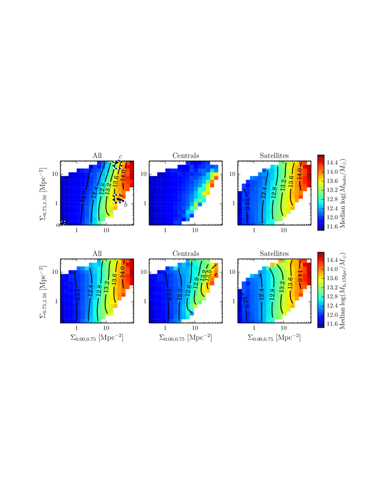
Figure 11: Top panels: halo mass dependence with density on scales $\Sigma_{0.00,0.75}$ and $\Sigma_{0.75,1.50}$ for all galaxies (left panels), central galaxies only (central panels) and satellite galaxies only (right panels) at $z=1.08$. Bottom panels: as before but the nominal halo mass has been replaced with that of the most massive halo within a 3D physical sphere of 1Mpc radius ($M_{\rm{h,1Mpc}}$). The labels $a$, $b$, and $c$ in the top left panel highlight three bins (black and white squares) whose halo mass distributions are shown in Figure 12.

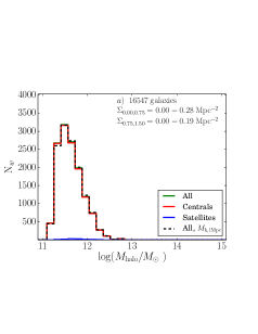
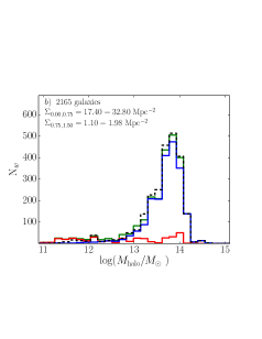
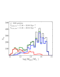
Figure 12: Halo mass distribution in three bins indicated using black and white squares and labelled $a$, $b$, and $c$ in the top left panel of Figure 11.

In order to understand these patterns it is important to roughly sketch the densities experienced by galaxies living in the core or in the outskirts of their own halo. A galaxy living in the centre of its own halo has high densities within annuli up to the size of the halo and low densities beyond. A galaxy living just beyond the halo virial radius has an intermediate density on small scales (as the aperture encompasses a fraction of the halo) and a high density on the larger scale, since the nearby halo core is located in this annulus. If we consider that those galaxies beyond the halo boundary are considered centrals, we fully understand why the density does not correlate positively with halo mass on large scales.

For the bottom panels of Figure 11 we show instead the mass of the most massive halo within 1 Mpc of each galaxy, $M_{\rm{h,1Mpc}}$. In contrast to the median mass of the parent halo, the mass of the most massive nearby halo correlates strongly with density for centrals (middle bottom panel). As already stressed in the text, the satellite galaxies are almost unaffected. The bottom left panel shows how the complete population behaves. The contours are now essentially vertical and the anti-correlation of halo mass with large-scale density at fixed small-scale density disappears.

We select three representative regions ($a$, $b$, $c$) in the upper left panel in Figure 11 and we study the distributions of halo mass in these regions in Figure 12).

The left-hand panel ($a$) shows the distribution of halo masses in the lowest density bin on both scales. Almost all the galaxies are centrals (red solid) living in low mass haloes and the halo mass replacement has little effect on the overall distribution (blue solid) as the majority of them have no neighbours within 1 Mpc. With the Millennium-II simulation we get the same result and so this is robust against resolution effects. The centre and right-hand panels ($b$ and $c$) are chosen to have the same high density on the inner 0.75 Mpc scale but very different densities in the outer annulus, highlighting the importance of the large-scale density. The galaxies whose large-scale density is low (panel b) live near the centre of their host halo, thus the sample is made almost entirely of satellites (blue solid) and the effect of centrals on the overall distribution is negligible. On the other hand, when $\Sigma_{0.75,1.50}$ is high (panel c), the contribution from centrals having halo masses smaller than $10^{12.5}M_{\odot}$ is 24%, causing a decrease in the median halo mass. This population of low halo mass centrals at high density can contain a significant population of “backsplash” galaxies, as discussed in Section 4. We see that the use of multiple scales can help identify such populations. Figure 11 also shows the distribution of $M_{\rm{h,1Mpc}}$ (black dashed lines) for our three bins: in panel c, the fraction of centrals with halo masses smaller than $10^{12.5}M_{\odot}$ is reduced to 10%. In this case the halo mass distribution is skewed to higher halo mass becoming similar to that in panel $b$.

References

- Abadi et al. (1999) Abadi, M. G., Moore, B., & Bower, R. G. 1999, MNRAS, 308, 947
- Angulo & White (2010) Angulo, R. E., & White, S. D. M. 2010, MNRAS, 405, 143
- Bahé et al. (2013) Bahé, Y. M., McCarthy, I. G., Balogh, M. L., & Font, A. S. 2013, MNRAS, 430, 3017
- Baldry et al. (2006) Baldry, I. K., Balogh, M. L., Bower, R. G., et al. 2006, MNRAS, 373, 469
- Balogh et al. (1997) Balogh, M. L., Morris, S. L., Yee, H. K. C., Carlberg, R. G., & Ellingson, E. 1997, ApJ, 488, L75
- Balogh et al. (2000) Balogh, M. L., Navarro, J. F., & Morris, S. L. 2000, ApJ, 540, 113
- Balogh et al. (2004) Balogh, M. L., Baldry, I. K., Nichol, R., et al. 2004, ApJ, 615, L101
- Blanton & Moustakas (2009) Blanton, M. R., & Moustakas, J. 2009, ARA&A, 47, 159
- Boselli & Gavazzi (2006) Boselli, A., & Gavazzi, G. 2006, PASP, 118, 517
- Boselli et al. (2008) Boselli, A., Boissier, S., Cortese, L., & Gavazzi, G. 2008, ApJ, 674, 742
- Boylan-Kolchin et al. (2012) Boylan-Kolchin, M., Bullock, J. S., & Kaplinghat, M. 2012, MNRAS, 422, 1203
- Bower et al. (2006) Bower, R. G., Benson, A. J., Malbon, R., et al. 2006, MNRAS, 370, 645
- Brammer et al. (2012) Brammer, G. B., van Dokkum, P. G., Franx, M., et al. 2012, ApJS, 200, 13
- Brough et al. (2011) Brough, S., Hopkins, A. M., Sharp, R. G., et al. 2011, MNRAS, 413, 1236
- Cole et al. (1994) Cole, S., Aragon-Salamanca, A., Frenk, C. S., Navarro, J. F., & Zepf, S. E. 1994, MNRAS, 271, 781
- Cole et al. (2000) Cole, S., Lacey, C. G., Baugh, C. M., & Frenk, C. S. 2000, MNRAS, 319, 168
- Cooper et al. (2005) Cooper, M. C., Newman, J. A., Madgwick, D. S., et al. 2005, ApJ, 634, 833
- Cooper et al. (2006) Cooper, M. C., Newman, J. A., Croton, D. J., et al. 2006, MNRAS, 370, 198
- Croton et al. (2005) Croton, D. J., Farrar, G. R., Norberg, P., et al. 2005, MNRAS, 356, 1155
- Croton et al. (2006) Croton, D. J., Springel, V., White, S. D. M., et al. 2006, MNRAS, 365, 11
- De Lucia & Blaizot (2007) De Lucia, G., & Blaizot, J. 2007, MNRAS, 375, 2
- De Lucia et al. (2004) De Lucia, G., Kauffmann, G., Springel, V., et al. 2004, MNRAS, 348, 333
- De Lucia et al. (2010) De Lucia, G., Boylan-Kolchin, M., Benson, A. J., Fontanot, F., & Monaco, P. 2010, MNRAS, 406, 1533
- De Lucia et al. (2012) De Lucia, G., Weinmann, S., Poggianti, B. M., Aragón-Salamanca, A., & Zaritsky, D. 2012, MNRAS, 423, 1277
- Dave et al. (1997) Dave, R., Hellinger, D., Primack, J., Nolthenius, R., & Klypin, A. 1997, MNRAS, 284, 607
- Dekel et al. (2003) Dekel, A., Devor, J., & Hetzroni, G. 2003, MNRAS, 341, 326
- Diemand et al. (2007) Diemand, J., Kuhlen, M., & Madau, P. 2007, ApJ, 667, 859
- Dressler (1980) Dressler, A. 1980, ApJ, 236, 351
- Elbaz et al. (2007) Elbaz, D., Daddi, E., Le Borgne, D., et al. 2007, A&A, 468, 33
- Fontanot et al. (2009) Fontanot, F., De Lucia, G., Monaco, P., Somerville, R. S., & Santini, P. 2009, MNRAS, 397, 1776
- Fossati et al. (2012) Fossati, M., Gavazzi, G., Boselli, A., & Fumagalli, M. 2012, A&A, 544, A128
- Franx et al. (2008) Franx, M., van Dokkum, P. G., Schreiber, N. M. F., et al. 2008, ApJ, 688, 770
- Gao et al. (2004) Gao, L., White, S. D. M.,Jenkins, A., Stoehr, F., & Springel, V. 2004, MNRAS, 355, 819
- Gavazzi et al. (2010) Gavazzi, G., Fumagalli, M., Cucciati, O., & Boselli, A. 2010, A&A, 517, A73
- Guo et al. (2011) Guo, Q., White, S., Boylan-Kolchin, M., et al. 2011, MNRAS, 413, 101
- Guo et al. (2013) Guo, Q., White, S., Angulo, R. E., et al. 2013, MNRAS, 428, 1351
- Gunn & Gott (1972) Gunn, J. E., & Gott, J. R., III 1972, ApJ, 176, 1
- Haas et al. (2012) Haas, M. R., Schaye, J., & Jeeson-Daniel, A. 2012, MNRAS, 419, 2133
- Henriques et al. (2013) Henriques, B. M. B., White, S. D. M., Thomas, P. A., et al. 2013, MNRAS, 431, 3373
- Hinshaw et al. (2013) Hinshaw, G., Larson, D., Komatsu, E., et al. 2013, ApJS, 208, 19
- Hirschmann et al. (2012) Hirschmann, M., Somerville, R. S., Naab, T., & Burkert, A. 2012, MNRAS, 426, 237
- Hirschmann et al. (2014) Hirschmann, M., De Lucia, G., Wilman, D., et al. 2014, arXiv:1407.5621
- Hogg et al. (2003) Hogg, D. W., Blanton, M. R., Eisenstein, D. J., et al. 2003, ApJ, 585, L5
- Kauffmann et al. (1993) Kauffmann, G., White, S. D. M., & Guiderdoni, B. 1993, MNRAS, 264, 201
- Kauffmann et al. (2004) Kauffmann, G., White, S. D. M., Heckman, T. M., et al. 2004, MNRAS, 353, 713
- Keel et al. (1985) Keel, W. C., Kennicutt, R. C., Jr., Hummel, E., & van der Hulst, J. M. 1985, AJ, 90, 708
- Kimm et al. (2009) Kimm, T., Somerville, R. S., Yi, S. K., et al. 2009, MNRAS, 394, 1131
- Knobel et al. (2012) Knobel, C., Lilly, S. J., Iovino, A., et al. 2012, ApJ, 753, 121
- Komatsu et al. (2011) Komatsu, E., Smith, K. M., Dunkley, J., et al. 2011, ApJS, 192, 18
- Kovač et al. (2010) Kovač, K., Lilly, S. J., Cucciati, O., et al. 2010, ApJ, 708, 505
- Kovač et al. (2013) Kovač, K., Lilly, S. J., Knobel, C., et al. 2013, arXiv:1307.4402
- Ilbert et al. (2009) Ilbert, O., Capak, P., Salvato, M., et al. 2009, ApJ, 690, 1236
- Lilly et al. (2013) Lilly, S. J., Carollo, C. M., Pipino, A., Renzini, A., & Peng, Y. 2013, ApJ, 772, 119
- Larson et al. (1980) Larson, R. B., Tinsley, B. M., & Caldwell, C. N. 1980, ApJ, 237, 692
- Ludlow et al. (2009) Ludlow, A. D., Navarro, J. F., Springel, V., et al. 2009, ApJ, 692, 931
- Madau et al. (1996) Madau, P., Ferguson, H. C., Dickinson, M. E., et al. 1996, MNRAS, 283, 1388
- Mamon et al. (2004) Mamon, G. A., Sanchis, T., Salvador-Solé, E., & Solanes, J. M. 2004, A&A, 414, 445
- McCarthy et al. (2007) McCarthy, I. G., Bower, R. G., & Balogh, M. L. 2007, MNRAS, 377, 1457
- Mo et al. (1998) Mo, H. J., Mao, S., & White, S. D. M. 1998, MNRAS, 295, 319
- Monaco et al. (2007) Monaco, P., Fontanot, F., & Taffoni, G. 2007, MNRAS, 375, 1189
- Muldrew et al. (2012) Muldrew, S. I., Croton, D. J., Skibba, R. A., et al. 2012, MNRAS, 419, 2670
- Muzzin et al. (2013) Muzzin, A., Marchesini, D., Stefanon, M., et al. 2013, ApJ, 777, 18
- Park et al. (2007) Park, C., Choi, Y.-Y., Vogeley, M. S., et al. 2007, ApJ, 658, 898
- Peng et al. (2010) Peng, Y.-j., Lilly, S. J., Kovač, K., et al. 2010, ApJ, 721, 193
- Peng et al. (2012) Peng, Y.-j., Lilly, S. J., Renzini, A., & Carollo, M. 2012, ApJ, 757, 4
- Perlmutter et al. (1999) Perlmutter, S., Aldering, G., Goldhaber, G., et al. 1999, ApJ, 517, 565
- The Planck Collaboration (2013) Planck Collaboration, Ade, P. A. R., Aghanim, N., et al. 2013, arXiv:1303.5076
- Poggianti et al. (1999) Poggianti, B. M., Smail, I., Dressler, A., et al. 1999, ApJ, 518, 576
- Poggianti et al. (2008) Poggianti, B. M., Desai, V., Finn, R., et al. 2008, ApJ, 684, 888
- Reid & Spergel (2009) Reid, B. A., & Spergel, D. N. 2009, ApJ, 698, 143
- Rodighiero et al. (2011) Rodighiero, G., Daddi, E., Baronchelli, I., et al. 2011, ApJ, 739, L40
- Saintonge et al. (2013) Saintonge, A., Lutz, D., Genzel, R., et al. 2013, ApJ, 778, 2
- Sandage (1986) Sandage, A. 1986, A&A, 161, 89
- Schechter (1976) Schechter, P. 1976, ApJ, 203, 297
- Scoville et al. (2013) Scoville, N., Arnouts, S., Aussel, H., et al. 2013, ApJS, 206, 3
- Shattow et al. (2013) Shattow, G. M., Croton, D. J., Skibba, R. A., et al. 2013, MNRAS, 433, 3314 .
- Skibba et al. (2011) Skibba, R. A., van den Bosch, F. C., Yang, X., et al. 2011, MNRAS, 410, 417
- Somerville & Primack (1999) Somerville, R. S., & Primack, J. R. 1999, MNRAS, 310, 1087
- Springel et al. (2001) Springel, V., White, S. D. M., Tormen, G., & Kauffmann, G. 2001, MNRAS, 328, 726
- Trinh et al. (2013) Trinh, C. Q., Barton, E. J., Bullock, J. S., et al. 2013, MNRAS, 436, 635
- Villalobos et al. (2013) Villalobos, Á., De Lucia, G., Weinmann, S. M., Borgani, S., & Murante, G. 2013, MNRAS, 433, L49
- Wang et al. (2006) Wang, L., Li, C., Kauffmann, G., & De Lucia, G. 2006, MNRAS, 371, 537
- Wang et al. (2008) Wang, J., De Lucia, G., Kitzbichler, M. G., & White, S. D. M. 2008, MNRAS, 384, 1301
- Wang et al. (2012) Wang, L., Weinmann, S. M., & Neistein, E. 2012, MNRAS, 421, 3450
- Weinmann et al. (2006) Weinmann, S. M., van den Bosch, F. C., Yang, X., & Mo, H. J. 2006, MNRAS, 366, 2
- Weinmann et al. (2009) Weinmann, S. M., Kauffmann, G., van den Bosch, F. C., et al. 2009, MNRAS, 394, 1213
- Weinmann et al. (2010) Weinmann, S. M., Kauffmann, G., von der Linden, A., & De Lucia, G. 2010, MNRAS, 406, 2249
- Weinmann et al. (2012) Weinmann, S. M., Pasquali, A., Oppenheimer, B. D., et al. 2012, MNRAS, 426, 2797
- Wetzel et al. (2013) Wetzel, A. R., Tinker, J. L., Conroy, C., & van den Bosch, F. C. 2013, arXiv:1303.7231
- Wilman et al. (2010) Wilman, D. J., Zibetti, S., & Budavári, T. 2010, MNRAS, 406, 1701
- Wilman et al. (2013) Wilman, D. J., Fontanot, F., De Lucia, G., Erwin, P., & Monaco, P. 2013, MNRAS, 433, 2986
- Whitaker et al. (2011) Whitaker, K. E., Labbé, I., van Dokkum, P. G., et al. 2011, ApJ, 735, 86
- Whitaker et al. (2012) Whitaker, K. E., van Dokkum, P. G., Brammer, G., & Franx, M. 2012, ApJ, 754, L29
- White & Rees (1978) White, S. D. M., & Rees, M. J. 1978, MNRAS, 183, 341
- White & Frenk (1991) White, S. D. M., & Frenk, C. S. 1991, ApJ, 379, 52
- Woo et al. (2013) Woo, J., Dekel, A., Faber, S. M., et al. 2013, MNRAS, 428, 3306
- Wright (2006) Wright, E. L. 2006, PASP, 118, 1711
- Yagi et al. (2010) Yagi, M., Yoshida, M., Komiyama, Y., et al. 2010, AJ, 140, 1814
- Yang et al. (2007) Yang, X., Mo, H. J., van den Bosch, F. C., et al. 2007, ApJ, 671, 153
- Yang et al. (2008) Yang, X., Mo, H. J., & van den Bosch, F. C. 2008, ApJ, 676, 248