CERN-OPEN-2014-050
Interpolation between multi-dimensional histograms using a new non-linear moment morphing method
M. Baaka, S. Gadatschb, R. Harringtonc, W. Verkerkeb
aCERN, Geneva, Switzerland
bNikhef, Amsterdam, The Netherlands
cUniversity of Edinburgh, Edinburgh, Scotland
-
Abstract
A prescription is presented for the interpolation between multi-dimensional distribution templates based on one or multiple model parameters. The technique uses a linear combination of templates, each created using fixed values of the model’s parameters and transformed according to a specific procedure, to model a non-linear dependency on model parameters and the dependency between them. By construction the technique scales well with the number of input templates used, which is a useful feature in modern day particle physics, where a large number of templates is often required to model the impact of systematic uncertainties.
1 Introduction
In particle physics experiments, data analyses generally use shapes of kinematical distributions of reconstructed particles to interpret the observed data. These shapes are simulated using Standard Model or other theoretical predictions, and are determined separately for signal and background processes. Simulations of known fundamental physics processes are run through a detailed detector simulation, and are subsequently reconstructed with the same algorithms as the observed data. These simulated samples may depend on one or multiple model parameters, for example the simulated Higgs particle mass, and a set of such samples may be required to scan over the various parameter values. Since Monte Carlo simulation can be time-consuming, there is often a need to interpolate between the limited number of available Monte Carlo simulation templates.
In particular, the statistical tests widely used in particle physics, e.g. for the construction of confidence intervals on model parameters or the discovery of new phenomena, rely strongly on continuous and smooth parametric models that describe the signal and background processes in the data111Typically, a statistical test involves the maximization of a likelihood function, which has been built from both the parametric model and the observed data. The maximization procedure relies on the derivatives of the likelihood with respect to the model’s parameters.. These parametric models describe parameters of interest, such as a shifting mass parameter or the rate of a signal process, and so-called nuisance parameters that parametrize the impact of systematic uncertainties. As such, the models are often constructed in terms of those parameters by interpolating between simulated Monte Carlo templates, thereby ensuring continuity in those parameters.
Several algorithms exist that can be used to interpolate between Monte Carlo sample distributions [1, 2]. Interpolation techniques have been used on multiple occasions in particle physics, for example to predict kinematic distributions for intermediate values of a model parameter, e.g. the simulated Higgs boson, boson or top quark mass, or to describe the impact of systematic uncertainties, which are often modeled as shape or rate variations about a nominal template of a kinematic distribution.
This work describes a new morphing technique, moment morphing, which has the advantage over existing methods in that it is fast, numerically stable, allows for both binned histogram and continuous templates, has proper vertical as well as horizontal morphing (explained in Section 2), and is not restricted in the number of input templates, the number of model parameters or the number of input observables. In particular, the latter feature allows the moment morphing technique to model the impact of a non-factorizable response between different model parameters, where varying one model parameter at a time is insufficient to capture the full response function.
The paper is organized as follows: Section 2 describes in detail how the moment morphing function, used to interpolate between histograms, is constructed using one or more morphing parameters. Section 3 describes how the moment morphing technique can be used to properly take into account systematic uncertainties in a high energy physics analysis, giving an example of a typical application. A comparison in terms of accuracy of moment morphing with alternative morphing algorithms is provided in Section 4. Section 5 describes the implementation of the moment morphing algorithm in publicly available C++ code, including benchmarking of its performance.
2 Construction of the morphing p.d.f.
This section details the construction of the moment morphing probability density function (p.d.f.). The method proposed here is based on the linear combination of input templates. The dependency on the morphing parameter(s) can be non-linear, and is captured in multiplicative coefficients and a transformation of the template observables. Interpolation using a single morphing parameter is described in Section 2.1. Section 2.2 describes interpolation using multiple morphing parameters and shows that dependencies between morphing parameters can be readily modeled. Other choices of basis functions for the construction of the morphing p.d.f. are considered in Section 2.3.
2.1 Interpolation with a single morphing parameter
Consider an arbitrary p.d.f. , where depends on the single morphing parameter and describes the observables . The true dependency on is not known or difficult to obtain. Instead, the p.d.f. has been sampled at different values of , with each representing a known input template shape for a single value of the morphing parameter, labeled . In the following the goal is to construct a parametric approximation of for arbitrary , which is continuous and smooth in the model parameter, as required for example by the statistical tests used in particle physics alluded to in Section 1. There are two steps to this.
First, given the sampling points, can be expanded in a Taylor series up to order around reference value ,
| (1) |
where the second equality defines . For the given values of follows the vector equation:
| (2) |
where defines a transformation matrix. Inverting Eqn. 2 gives
| (3) |
which allows to determine the values . Substituting this in Eqn. 1, reads
| (4) |
which can be used to predict the template shape at any new value of the morphing parameter given by ,
| (5) |
which is a linear combination of the input templates , each multiplied by a coefficient ,
| (6) |
which themselves are non-linear and depend only on the distance to the reference points. This approach of weighting the input templates is also known as vertical morphing. Note that the coefficients are independent of the derivatives of with respect to morphing parameters or to the observable set , making their computation easy.
The coefficient for a point included in the set of input templates is one, i.e.
| (7) |
and by construction the sum of all coefficients equals one:
| (8) |
This turns out to be a useful normalization, as will be seen below.
To illustrate, one can consider a morphed p.d.f. using only input templates at two values of the morphing parameter, and . The coefficients become linear in and reduce to the simple fractions:
| (9) | |||||
| (10) |
where , and sum up to one, and all other coefficients are zero.
Second, it may be that the sampled input p.d.f.s describe distributions in that vary strongly as a function of in shape and location. This is equivalent to the first and second moments (i.e. the means and variances) of the input distributions having a dependence on the morphing parameter .
Since the input p.d.f.s in Eqn. 5 are summed linearly, it is imperative to translate all input distributions in the sum before combining in the morphed p.d.f. such that their locations match up. The process of translating the input observables (but not scaling; see below) is also called horizontal morphing. In addition it is necessary to take in account the change in the width of the input distributions as a function of the morphing parameter.
To achieve this, the mean and width of each input distribution and observable are shifted to the common values of and . These are obtained by multiplying the underlying means and widths with the coefficients of Eqn. 6
| (11) | ||||
| (12) |
In order to shift the input p.d.f.s a linear transformation of each observable is applied. For each p.d.f. and observable define
| (13) |
with slope
| (14) |
and offset
| (15) |
to replace the original observables in the input p.d.f.s
| (16) |
Since only a linear transformation is applied to each observable, i.e. only the first two moments of the input p.d.f.s are modified, the normalization of the scaled input template is analytically related to the normalization of the original template as
| (17) |
with the slope , where refers to the observable . The construction of the complete morphed p.d.f. as the sum of the transformed input p.d.f.s then gives
| (18) |
As the coefficients add up to by construction, the morphed p.d.f. of Eqn. 18 is unit-normalized as well for normalized input templates.
This leads to an important computational advantage and novelty: for models where the input templates are constant, such as histogram-based templates, no normalization integrals need to be recalculated during the minimization of the likelihood function, which is often a bottle-neck when using morphed p.d.f.s. As a result, the number of input templates is generally increasable without significant performance loss.
Note that the self-normalization of Eqn. 17 remains valid when applying a rotation to the set of (multiple) observables, which would introduce covariance moments to the modified input p.d.f.s. Though technically possible, such rotations are avoided here as they obscure the physical interpretation of the observable set. A consequence of this on the accuracy of the morphed p.d.f. to model changing correlations between observables is discussed in Section 4.2.
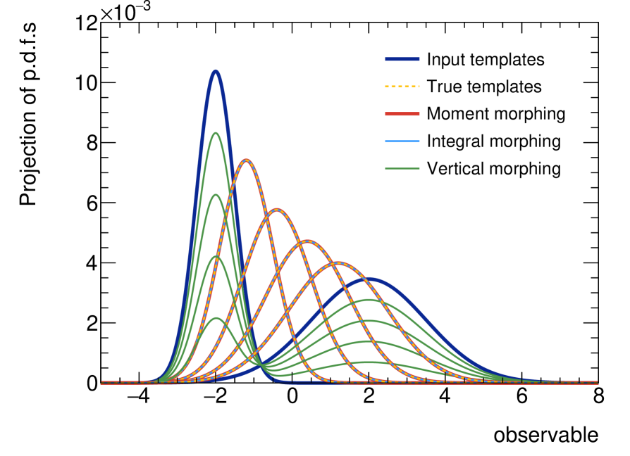
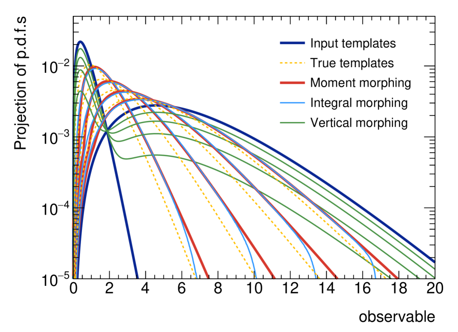
The processes of vertical and horizontal morphing (i.e. summing and translating) and of scaling the input morphed p.d.f.s are illustrated in Fig. 1, which morphs between two normal distributions. The technique proposed also accurately models the evolution of rapidly changing distributions as illustrated in Fig. 1. In the sample, the application of moment morphing is used to describe the non-linear transition of a Cauchy distribution via a Crystal Ball line shape into a normal distribution. The parameters of the used p.d.f.s are chosen such that the positions of their means as well as their shapes vary substantially as a function of the morphing parameter , in particular in the tails of the distributions which change dynamically along the morphing path.
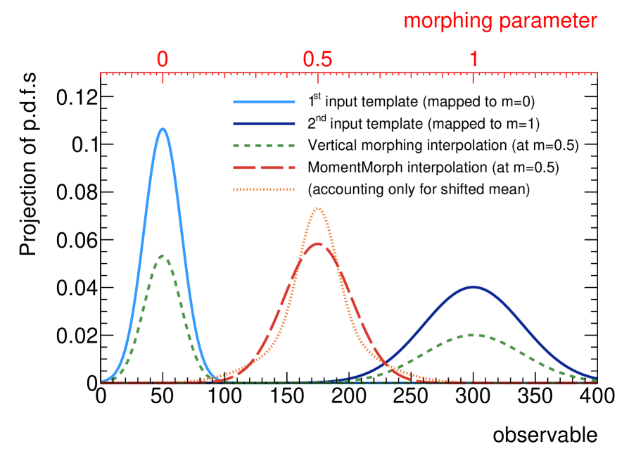
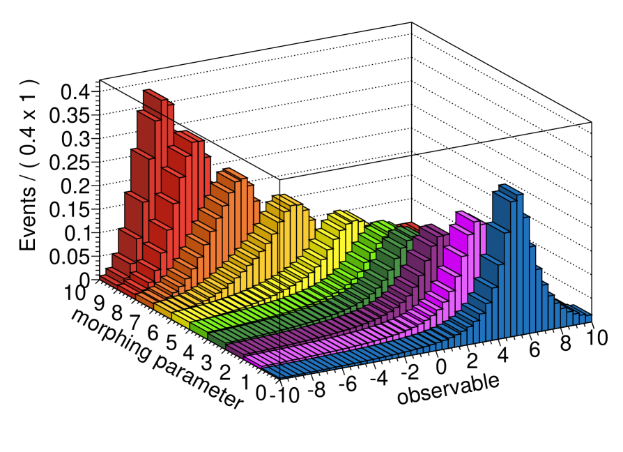
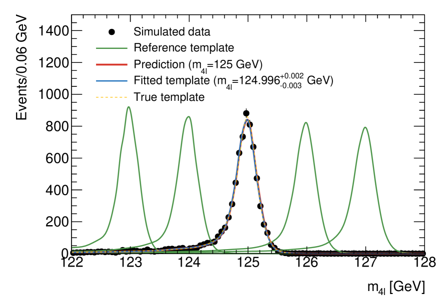
Fig. 2 shows an application of the technique described in this article to a complex physics and detector simulation. The reconstructed invariant mass distribution for a Standard Model Higgs boson with mass decaying to four leptons is described by non-linearly interpolating between a series of templates corresponding to simulation response estimates for four assumed Higgs boson masses, at , , and . As reference templates kernel estimation p.d.f.s modeling events simulated with MadGraph [3] and an ATLAS-type PGS [4] simulation are used. Despite rapidly evolving features, the template predicted by the morphing technique reproduces the true template at . The resulting morphed p.d.f. is parametrized in terms of the “true” Higgs boson mass, as opposed to the reconstructed invariant mass, and a fit of the morphed p.d.f. to a dataset with an assumed true Higgs boson of directly and accurately measures that true Higgs boson mass.
2.2 Interpolation with multiple morphing parameters
The non-linear implementation of multiple morphing parameters is analogous to the single parameter case of Section 2.1. We illustrate here the expansion to two parameters, including correlated effects in the template distribution caused by changing of two or more morphing parameters simultaneously, before generalizing the approach to an arbitrary number of parameters.
The general Taylor series expansion of , depending on parameters and , around reads:
| (19) |
which, for a square grid with reference points surrounding , is approximated by:
| (20) |
Here the middle two terms are the linear expansions along and , and the last term represents the expansion along both and simultaneously. The addition of the fourth “corner” point allows one to model functions that cannot be factorized into functions depending only on or .
Repeating the Taylor series expansion for a grid of reference points, and again writing the truncated series as a vectorial equation, leads to Eqn. 2 with additional mixed terms in the transformation matrix and the derivatives . The transformation matrix now reads
| (21) |
where is a short notation for the distance between reference point and reference point in the dimension of the parameter space. The distance vector is in multiple dimensions defined as
| (22) |
Following Eqn. 5, the coefficients for a new point are now given by
| (23) |
The construction of the morphed p.d.f. using these coefficients is as in Eqn. 18.
The extension to an arbitrary number of morphing parameters, , is a matter of using an -dimensional grid of input p.d.f.s, with grid points, and consistently expanding the transformation matrix with the additional higher order terms.
Returning to the square grid of input p.d.f.s with reference values surrounding , the coefficients in reduce to
| (24) | |||||
| (25) | |||||
| (26) | |||||
| (27) |
with and . Note that the coefficients are all positive when staying within the boundaries of the grid, and add up to . Towards the corner point , the nominal coefficient and linear-expansion coefficients and are turned off, and the quadratic term in is turned on in full, describing the change caused by changing and simultaneously.
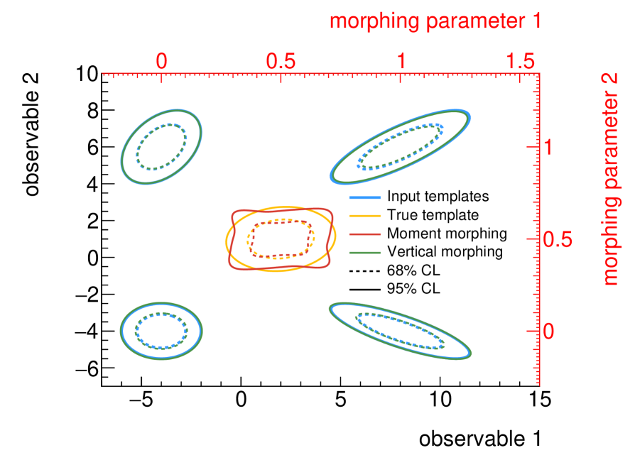
Shown in Fig. 3 is an illustration of a multivariate normal distribution modeling the dependency between two observables. The covariance matrix as well as the mean change as a function of two parameters and . In the given example the distributions are known for grid points fulfilling . The information is used to linearly interpolate the p.d.f. to any desired point in the two-dimensional parameter space. The yellow contours in the center of the grid, i.e. at , represent the true template, which is compared with the prediction by the moment morphed p.d.f. (red) and the prediction by vertical morphing only (green). Similar to the example presented in Fig. 1, vertical morphing only does not yield a central template with shifted mean. The difference between the moment morphed template and the true template is induced by the change of the correlation between the two observables with varying morphing parameter values. In case of constant correlation between the observables of the input templates, the prediction of the moment morphed p.d.f. is exact. More discussion on this follows in Section 4.2.
2.3 Other choices of basis functions
Finally, having derived the morphed p.d.f. using a Taylor series expansion, the dependency on a morphing parameter can be easily re-expressed in any orthonormal basis . The choice of the basis functions can simplify the studied problem and thus lead to a better approximation, even to an exact description. For example, if the dependency on model parameters is expected to be periodic, it can be expressed in Fourier space as a linear combination of the eigenvectors :
| (28) |
where the coefficients read
| (29) |
Thus, the dependency of the morphed p.d.f. on the observables enters through the coefficients only, while the basis functions are independent of .
Note that the number of sampling points limits the number of utilizable basis functions . Analogously to Eqn. 5, can then be predicted at any new point ,
| (30) |
with the modified transformation matrix .
3 A p.d.f. for modeling systematic uncertainties
In a typical analysis performed in a particle physics experiment, the impact of systematic uncertainties is typically quantified by varying one-by-one the model parameters relating to detector modeling and physics models (e.g. energy calibrations, factorization scales) and to record the template distribution with these modified settings. The resulting pairs of alternate templates, corresponding to “up” and “down” variations of the uncertain model parameters, must then be incorporated in the likelihood model of the physics analysis, in the form of a model nuisance parameter that causes the template distribution to deform as prescribed by the pair of “alternate” templates.
For the most widely-used statistical test at the LHC, the profile likelihood ratio, it is required that the modeling of the systematic uncertainty in terms of a nuisance parameters is done in a continuous way. In particular, the maximization of the likelihood function, as needed (twice) in the profile likelihood ratio, requires continuous and smooth parametric models to describe the signal and background processes present in the data222Specifically, the likelihood for a physics measurement, , where is the physics parameter of interest and are the nuisance parameters that parametrize the impact of systematic uncertainties on the signal and background predictions, must be defined for all values of and . The profile likelihood ratio is given by (31) where and represent the unconditional maximum likelihood estimates of and , and represents the conditional maximum likelihood estimate for the chosen value of . Therefore is a function of . (Note that the data is omitted in the short hand notation of .) For a more detailed discussion on the profile likelihood ratio test statistic, see Ref. [5]..
This section builds a parametrized p.d.f. describing a set of systematic variations about the nominal prediction for a signal or background process, using the morphing technique of Section 2. Each systematic uncertainty is described with a nuisance parameter, , that continuously morphs between the variation and nominal templates such that corresponds to the ( = 1 standard deviation) variations, and corresponds to the nominal template333 A Gaussian constraint is applied separately for each systematic uncertainty to account for uncertainty in the external measurement. This constraint preferably centers each systematic variation around the nominal prediction, with a reduced likelihood for potential shifts; however, a combined fit to the observed data may of course prefer shifts in the nuisance parameters.. Additional variation templates may be added for different values of .
The response of the likelihood function to changes in the nuisance parameters is here assumed to be factorized, i.e. it is assumed that the effect of a simultaneous changes in two or more nuisance parameters can be described as a superposition of the effects of changing each nuisance parameter individually. (Unfactorizable uncertainties are not discussed here; their treatment is handled following the recipe of Section 2.2.) Where unfactorizable uncertainties would require a full -dimensional grid of input templates, this assumption reduces the number of required inputs to a set of one-dimensional variations, with only the nominal template in common – a “star” shape in the nuisance parameter space.
The construction of the morphed p.d.f. as the sum of the input templates becomes
| (32) |
where the double-sum runs over the implemented systematic uncertainties and their available variations. The morphed p.d.f. is self-normalized, as by construction all coefficients add up to one.
In the publicly available implementation, detailed in Section 5.1, the coefficients are linear, and depend only the two closest input points surrounding , as in Eqn. 9. Also, the linear transformation of the observables , responsible for scaling and horizontal morphing, can be turned on or off. (By default it is off.) Henceforth this p.d.f. is called the star-morphed p.d.f.
This type of star-morphed p.d.f. has been used in the analysis of Higgs decay to 4 leptons () by the ATLAS experiment [6] to describe the various background components contributing the mass spectrum, each including the variations of all relevant systematic uncertainties.
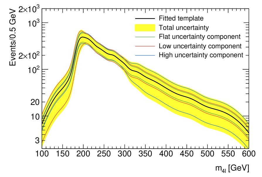
Fig. 4 shows an example application of the star-morphed p.d.f., used to describe the dominant background process for a typical analysis, labeled . As in Section 2.1, this background prediction has been obtained from events simulated with MadGraph [3] and PGS [4]. For illustration, three non-physical systematic uncertainties have been added to the star-morphed p.d.f. One is a shape variation in the low mass region, the second is a shape variation in the high mass region, and the third is an overall normalization uncertainty that affects the entire mass region. The effects of these systematic uncertainties on the template distribution are shown in Fig. 4.
4 Accuracy of moment morphing and comparison to alternative morphing algorithms
The accuracy of a moment morphing function is assessed here using a series of benchmark models for which the true distribution is defined.
A priori one can demonstrate that moment morphing provides an exact solution for any set of true distributions in which the first and second moment (i.e. the mean and width) of change linearly with the morphing parameter and all other moments are constant (i.e. the shape of the distribution does not change other than through its first and second moment). The simplest example of such a distribution is a Gaussian distribution with a linearly changing mean and width. However, the class of true distributions that are exactly reproduced by moment morphing is not restricted to this example: any distribution with linearly changing first and second moments and fixed higher-order moments is exactly described. In particular, when considering use cases in particle physics, the physics parameters of interest (particle masses, resonance widths, etc.) are often related to the first and second moments; hence a correct description of these is most critical.
Deviations from the exact solution can occur in two ways: a) the dependence of the first and second moment of become non-linear in , or b) higher moments of the shape of the distribution depend on , either linearly or non-linearly. The magnitude of both types of deviations are under explicit control of the user, as the moment morphing algorithm allows templates to be specified at any number of freely choosable values of .
Deviations of the first type are generally unproblematic as it is always possible to construct a configuration of templates in which: a) the dependence of the first and second moments between any pair of adjacent templates is sufficiently close to linear (when choosing the piece-wise linear interpolation option), or b) where the dependence of the moments over the entire domain of is well approximated by a -order polynomial for templates (when choosing the non-linear interpolation option). For this reason, no attempt is made here to quantify the accuracy of moment morphing due to (local) non-linearity of the first and second moment of .
Deviations of the second type, introduced by changing higher-order moments, may be more limiting in cases where higher-order moments of the true distribution change rapidly as a function of . It should be noted that changes in the truth distribution related to higher-order moments are empirically accounted for in the morphing algorithm, by gradually changing the weight of moment-adjusted input templates as a function of . However, the morphed distribution does not guarantee a linear change in these higher-order moments as a function of , as is done for the first and second moments.
The impact of this empirical modelling of changes in higher-order moments is quantified in the following sub-sections.
4.1 Performance on benchmark models
The accuracy of moment morphing is evaluated here on nine analytical benchmark models that are similar to various particle physics use cases, and the accuracy is compared to two other morphing algorithms that have historically been used in particle physics: vertical morphing and “integral morphing”.
In the vertical morphing approach444Note that the moment morphing algorithm reduces to vertical morphing strategy if the adjustment step of the first and second moments of the input templates is omitted. templates are interpolated with a simple weighting strategy:
where are the left and right template models corresponding to . The vertical morphing approach is widely used in LHC physics analyses, notably in the modeling of distributions in the discovery analysis of the Higgs boson. In contrast, in the integral morphing approach [1] interpolation occurs between the cumulative distribution functions of the templates . The integral morphing approach is more suited to models with rapidly shifting means, like moment morphing and unlike vertical morphing, but is computationally intensive due to (numeric) integration and root-finding steps, and is restricted to the description of one-dimensional distributions. The integral morphing approach has been used, among others, in physics analyses published by the D0 and CDF collaborations.
| Name | Model description | Dependence on morphing parameters | |
|---|---|---|---|
The nine analytical benchmark models tested here are detailed in Table 1. For the first three benchmark models and , based on the normal distribution, moment morphing provides an exact solution, and these models are included in the benchmark to facilitate accuracy performance comparisons with the other morphing approaches. The second set of benchmark models is based on the Gamma distribution:
and are included as an example of a distribution where also higher-order moments of the true distribution changes as a function of the morphing parameter. The last set of three benchmark models is based on the -order Chebychev polynomials:
as a distribution that is representative of typical background distributions.
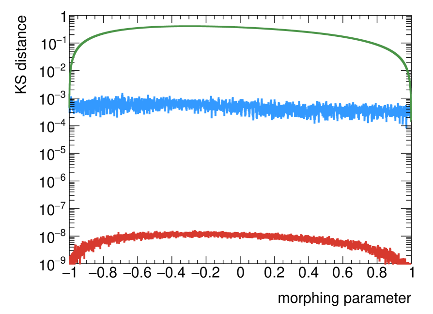
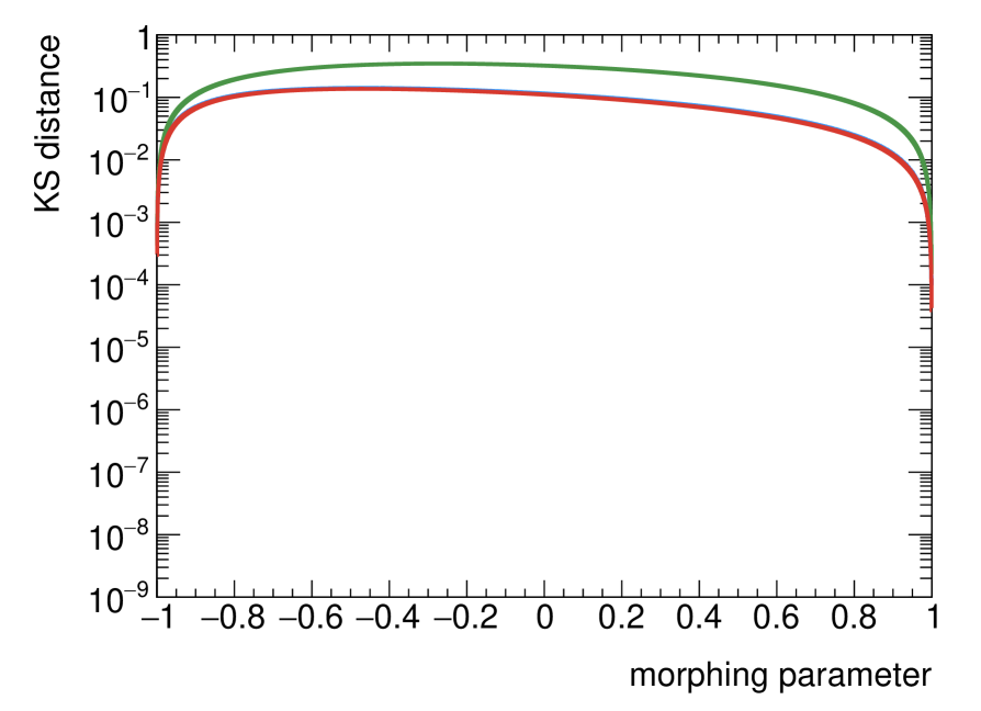
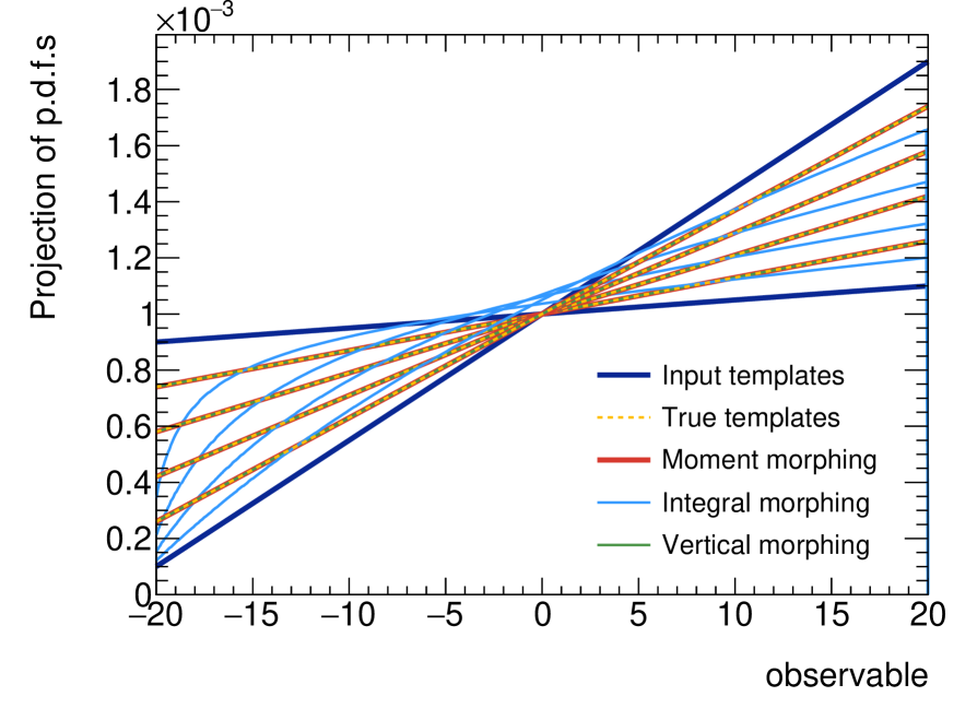
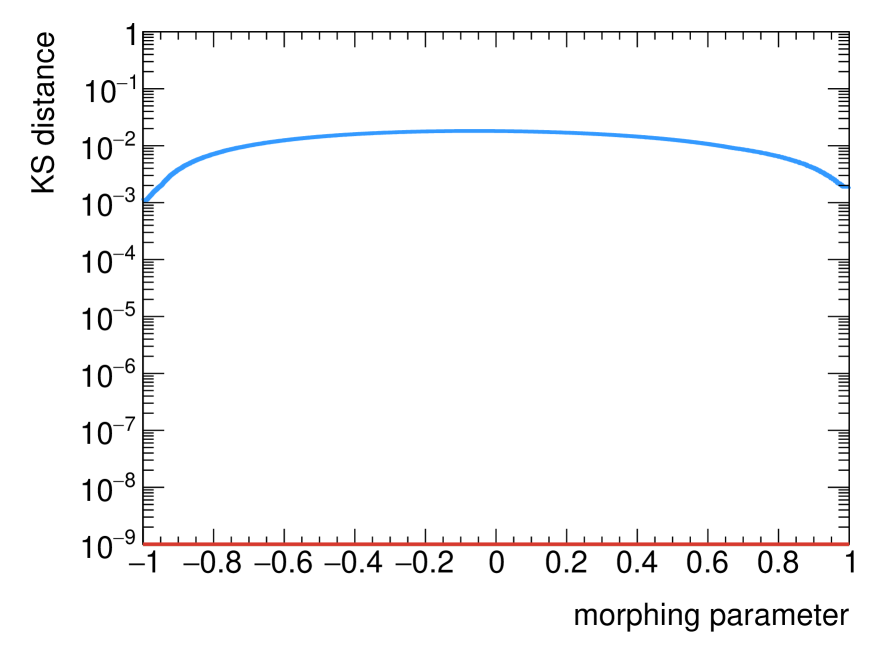
Given a pair of input templates positioned at , the accuracy of the morphing methods is quantified using the Kolmogorov-Smirnov (KS) distance. This is the largest distance between the cumulative distribution functions of the truth model and the cumulative distribution function of the morphing interpolation model for any value of , as a function of the morphing parameter . The KS distance values range between zero (perfect agreement between the two distributions) and one (complete spatial separation of the distributions in ).
| Moment morphing | Vertical morphing | Integral morphing | ||||
|---|---|---|---|---|---|---|
| Name | ||||||
| 0.018 | ||||||
Fig. 5 illustrates the accuracy of the three morphing approaches on the and models, along with the KS statistic as a function of for all morphing approaches. Accuracy metrics for all nine benchmark models are given in Table 2, which summarizes for each benchmark model and each morphing strategy the KS distance at (the morphing mid-point), and the worst KS distance that occurs in the morphing range .
As expected, the moment morphing approach exactly replicates the benchmark model, unlike the vertical morphing approach. The integral morphing algorithm can also exactly replicate the model, but is limited to an accuracy of about 0.001 due to numerical precision limitations, related to integration and root-finding in the algorithm’s implementation. For the benchmark model, no morphing algorithm can exactly reproduce the truth model due to changing higher-order moments, but the moment and integral morphing algorithms perform about equally, and significantly better than the vertical morphing algorithm. For the benchmark model both the moment morphing and vertical morphing perform identically, as the first and second moment of the true distribution do not depend on , hence both approaches reduce to the same algorithm, which happens to describe the model perfectly555This perfect performance is specific to the benchmark that changes the first Chebychev coefficient only. Truth models that change high-order coefficients are imperfectly described my all morphing algorithms, as detailed in Table 2..
In summary, in these tests the moment morphing approach is as good as and usually better than the two alternative morphing methods.
4.2 Accuracy for multi-dimensional distributions and multi-parameter morphing
For morphing models with multiple morphing parameters, and/or with input distributions with multiple observables, it is challenging to capture the accuracy with a limited set of benchmark models as KS tests have no simple equivalent for multidimensional distributions, and the number of benchmark permutations to test becomes large with multiple morphing parameters.
Nevertheless, one can illustrate the challenges of morphing and the performance of moment morphing with a single simple yet challenging 2-parameter benchmark model for 2-dimensional distributions: a multivariate normal distribution:
for which all five degrees of freedom, and depend linearly on two morphing parameters .
In the case where the correlation coefficient is independent of , moment morphing provides the exact solution for this multi-variate Gaussian model, similar to the one-dimensional case, even if the dependence of is strong, as long as it is linear. Conversely, vertical morphing will perform poorly, especially if or depend strongly on , while integral morphing is not available for multi-dimensional distributions.
The more challenge scenario where also depends on is visualized in Fig. 3. Moment morphing will not provide an exact solution for this class of models as the covariance moments are not explicitly corrected for, nevertheless the covariance of the interpolated shape at reasonably matches the covariance of the true model, although the shape is no longer perfectly Gaussian.
5 Implementation
This section discusses the publicly available morph classes, and is followed by details of the chosen extrapolation approach of a morph parameter beyond the provided input range.
5.1 Available morph classes
Moment morphing has been implemented in C++ for the RooFit toolkit [7]. As of ROOT release 5.34.22, the morphing features described in this document are available in the RooFit models library. Common to all classes is the ability to handle one or multiple observables, as well as the implementation of a cache that stores pre-calculated expensive components such as numerically computed moments, e.g. the means and widths of each input template, required for the translation of the corresponding observables.
The following moment morph classes are available in RooFit.
-
•
The RooMomentMorph p.d.f. can be used to interpolate between an arbitrary number of reference distributions using a single morphing parameter. The algorithms settings described in this paper, e.g. linear or truly non-linear, can be used.
Furthermore, a sine-linear variant transforms to before calculating the coefficients, thus ensuring a continuous and differentiable transition when crossing between two adjacent sets of enclosing grid points. In addition, non-linear coefficients for adjusting the moments of the p.d.f.s can be mixed with linear coefficients when constructing the morph p.d.f., and an option is available to select positive non-linear coefficients only.
-
•
RooStarMomentMorph is the natural extension for combining multiple one-dimensional RooMomentMorph p.d.f.s with one common sampling point. The class supports linear and sine-linear interpolation. The transformation of the template observables can be turned on or off.
-
•
RooMomentMorphND allows the parametrization of a -dimensional parameter space, interpolating linearly or sine-linearly between reference points sitting on a hyper-cube or arbitrary size.
-
•
Roo1DMomentMorphFunction and Roo2DMomentMorphFunction are similar to the top moment morph p.d.f., but can be used to interpolate between functions, not p.d.f.s. Available for one or two morph parameters.
Example code of how to use the moment morph p.d.f. is given below.
5.2 Extrapolation beyond input boundaries
By construction, the validity of the morph p.d.f. of Eqn. 18 is highest when interpolating its morph parameter(s) within the provided range(s) of input values. Beyond these the predictive power is a priori unknown, but of course can be interesting to investigate. Some ad hoc choices need to be made for extrapolation cases, which were not covered by the description of the algorithm so far.
As apparent from Eqn. 6, when extrapolating beyond the input boundary values and , the coefficients increase in size and may become highly negative. In this situation the morph p.d.f. can become smaller than zero, and as such ill-defined. To prevent this, the following extrapolation approach is implemented.
-
•
Whenever one of the morph parameters extends beyond the input range, i.e. or , the coefficient multiplied with the nearest input p.d.f. is forced to one, and all other coefficients are set to zero.
-
•
The same is done for the transformed width of Eqn. 11, which is to remain greater than zero.
- •
5.3 Computational performance of moment morphing
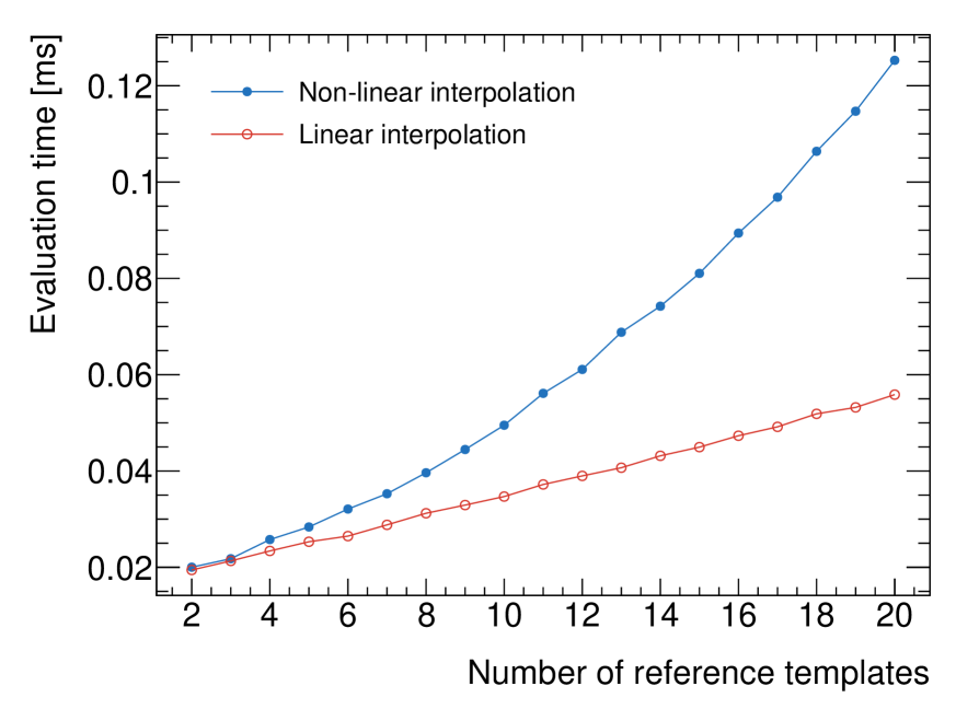
Template morphing is one of the computationally limiting factors in current HEP analyses, which makes understanding the performance of the algorithm at hand crucial. Fig. 6 compares the performance of the linear and non-linear algorithms settings in terms of average CPU time needed for the evaluation of the morph p.d.f. as a function of the used reference templates. The benchmark makes use of the caching described in section 5.1. It excludes the computation time needed for the calculation of the moment integrals over the input templates, which is a one-time calculation, the result of which can be cached in the RooFit workspace file along with the model if desired by the user. Details of the setup are described in the caption of the figure.
For the interpretation of performance numbers it should be noted that the evaluation time for non-linear morphing models depends quadratically on the number of reference templates , as for every template the associated coefficient is a product of distances. In the linear case, the evaluation time is driven by the efficiency of the algorithm finding the two closest reference points surrounding the point at which the p.d.f. is evaluated. For () reference templates, the ratio of non-linear over linear evaluation time is ().
6 Conclusion
We have described a new algorithm to interpolate between Monte Carlo sample distributions, called moment morphing. The proposed technique is based on a linear combination of the input templates, has a non-linear dependence on the parameters that control the morphing interpolation, and can be constructed in any orthogonal basis.
Compared with existing methods, it allows for both binned histogram and continuous templates, has both horizontal and vertical morphing, and is not restricted in the number of input templates, observables, or model parameters. In particular, the latter feature allows the moment morphing technique to model the impact of a non-factorizable response between different model parameters. The moment-morphed p.d.f. is self-normalized, and therefore, in terms of speed and stability, scales well with the number of input templates used. This is a useful feature in modern day particle physics where large numbers of templates are often required to model the variations by systematic uncertainties.
In a suite of comparison tests the moment morphing method proofs to be as accurate as, or better than, two commonly used alternative techniques.
Various implementations of the moment morphing technique are publicly available through the RooFit toolkit.
Acknowledgments
This work was supported by CERN, Switzerland; FOM and NWO, the Netherlands; and STFC, United Kingdom.
References
- [1] A. L. Read, “Linear interpolation of histograms”, Nucl.Instrum.Meth. A425 (1999) 357–360.
- [2] K. Cranmer, G. Lewis, L. Moneta, A. Shibata, W. Verkerke, “HistFactory: A tool for creating statistical models for use with RooFit and RooStats”, CERN-OPEN-2012-016.
- [3] J. Alwall, R. Frederix, S. Frixione, V. Hirschi, F. Maltoni, et al., “The automated computation of tree-level and next-to-leading order differential cross sections, and their matching to parton shower simulations”, arXiv:1405.0301.
- [4] J. Conway, et al., http://www.physics.ucdavis.edu/conway/research/software/pgs/pgs4-general.htm.
- [5] G. Cowan, K. Cranmer, E. Gross, O. Vitells, “Asymptotic formulae for likelihood-based tests of new physics”, Eur.Phys.J. C71 (2011) 1554. arXiv:1007.1727.
- [6] G. Aad, et al., “Measurements of Higgs boson production and couplings in the four-lepton channel in pp collisions at center-of-mass energies of 7 and 8 TeV with the ATLAS detector”, arXiv:1408.5191.
- [7] W. Verkerke, D. P. Kirkby, “The RooFit toolkit for data modeling”, eConf C0303241 (2003) MOLT007. arXiv:physics/0306116.