Flexible Modeling of Epidemics
with an Empirical Bayes Framework

Logan C. Brooks¹ David C. Farrow¹ Sangwon Hyun² Ryan J. Tibshirani² Roni Rosenfeld¹ Roni.Rosenfeld@cs.cmu.edu

( ¹School of Computer Science, Carnegie Mellon University,
Pittsburgh, Pennsylvania, United States of America
²Department of Statistics, Carnegie Mellon University,
Pittsburgh, Pennsylvania, United States of America )

1 Abstract

Seasonal influenza epidemics cause consistent, considerable, widespread loss annually in terms of economic burden, morbidity, and mortality. With access to accurate and reliable forecasts of a current or upcoming influenza epidemic’s behavior, policy makers can design and implement more effective countermeasures. This past year, the Centers for Disease Control and Prevention hosted the “Predict the Influenza Season Challenge”, with the task of predicting key epidemiological measures for the 2013–2014 U.S. influenza season with the help of digital surveillance data. We developed a framework for in-season forecasts of epidemics using a semiparametric Empirical Bayes framework, and applied it to predict the weekly percentage of outpatient doctors visits for influenza-like illness, as well as the season onset, duration, peak time, and peak height, with and without additional data from Google Flu Trends. Previous work on epidemic modeling has focused on developing mechanistic models of disease behavior and applying time series tools to explain historical data. However, these models may not accurately capture the range of possible behaviors that we may see in the future. Our approach instead produces possibilities for the epidemic curve of the season of interest using modified versions of data from previous seasons, allowing for reasonable variations in the timing, pace, and intensity of the seasonal epidemics, as well as noise in observations. Since the framework does not make strict domain-specific assumptions, it can easily be applied to other diseases as well. Another important advantage of this method is that it produces a complete posterior distribution for any desired forecasting target, rather than mere point predictions. We report prospective influenza-like-illness forecasts that were made for the 2013–2014 U.S. influenza season, and compare the framework’s cross-validated prediction error on historical data to that of a variety of simpler baseline predictors.

2 Author Summary

Influenza epidemics occur annually, and incur significant losses in terms of lost productivity, sickness, and death. Policy makers employ countermeasures, such as vaccination campaigns, to combat the occurrence and spread of infectious diseases, but epidemics exhibit a wide range of behavior, which makes designing and planning these efforts difficult. Accurate and reliable numerical forecasts of how an epidemic will behave, as well as advance notice of key events, could enable policy makers to further specialize countermeasures for a particular season. While a large amount of work already exists on modeling epidemics in past seasons, work on forecasting is relatively sparse. Specially tailored models for historical data may be overly strict and fail to produce behavior similar to the current season. We designed a framework for predicting epidemics without making strong assumptions about how the disease propagates by relying on slightly modified versions of past epidemics to form possibilities for the current season. We report forecasts generated for the 2013–2014 influenza season, and assess its accuracy retrospectively.

3 Introduction

Seasonal influenza epidemics occur each year and incur significant economic burden, morbidity, and mortality. The annual impact in the United States has been estimated at $611{\mathrm{K}}$ lost undiscounted life-years, $3.1{\mathrm{M}}$ hospitalized days, $31.4{\mathrm{M}}$ outpatient visits, and $\$87.1{\mathrm{B}}$ in economic burden [1]. Accurate and reliable forecasts offer many opportunities to improve preparedness and response to influenza epidemics. Long-term predictions could be used to help select a vaccine for the next season. Forecasts within a season can help policy makers to tailor vaccination campaigns and advisories, hospitals to prepare staff and beds, and individuals and organizations to plan for vaccination and potential sickness. Despite the notable impacts of the disease, though, many weaknesses of influenza surveillance and prediction systems in the past [2] remain today. Capabilities to observe and forecast the prevalence of influenza and similar diseases lag considerably, e.g., behind analogues in meteorology. During the 2013–2014 flu season, the CDC hosted the “Predict the Influenza Season Challenge”, which encouraged teams to forecast features of the current epidemic progression that would be useful to policy makers, and to take advantage of digital surveillance such as search engine and social network data. The competition established a closer relationship between forecasters and policy makers, and provided valuable assessment of the performance of true (prospective) within-season forecasts.

Existing work on modeling influenza epidemic curves generally falls into one of three categories:

Compartmental models: estimate the number of people in various states related to a disease [3]. For example, the SIR model approximates dynamics between the proportions of the population susceptible to influenza, infected with the virus, and recovered from infection. Common assumptions include that any pair of individuals in a population are equally likely to interact, and that different strains of influenza behave identically.
Agent-based models: generate synthetic populations based on census data and build complex schemes of interaction and disease behavior in synthetic humans [4, 5, 6, 7, 8]. It is common for these systems to be applied to the special case of a single, novel strain of influenza.
Parametric statistical models: are tools from time series modeling that are less closely tied with mechanistic assumptions of how flu is transmitted. Simple approaches include linear autoregression, which estimates flu activity at some time with a linear function of the flu activity in the recent past. More complex alternatives include Box-Jenkins analysis, generalized linear models (GLM), and generalized autoregressive moving-average models [9].

Past forecasting efforts [10, 11] usually take a compartmental model [12, 13], agent-based model, or parametric statistical model [14, 15, 16], and condition on partial data to predict flu activity levels one to ten weeks in the future. Other methods include prediction markets [17], which combine expert predictions using a stock market-like system, and the method of analogues ( $k$ nearest neighbors) [18], which makes predictions of future flu activity levels using similar patterns from the past, without assuming a strict model.

We take a nonmechanistic approach, generating possibilities for the current season’s epidemic curve using modified versions of past seasons’ curves, incorporating reasonable adjustments in the timing, pace, and intensity of the epidemic, as well as accommodating noise in observations. Our method differs from the mechanistic and parametric statistical model approaches in that it models the process generating the data nonparametrically, rather than using a model that may significantly misrepresent the data. While the method of analogues is similar in this regard as a nonparametric method, our framework considers the entire season as a unit, which differs from the traditional perspective in nearest neighbor modeling. Our framework also models the error in observations, and outputs a distribution rather than point predictions, while existing applications of the method of analogues generate single point predictions one at a time.

4 Materials and Methods

4.1 Surveillance data

4.1.1 U.S. Outpatient Influenza-like Illness Surveillance Network (ILINet)

The Centers for Disease Control and Prevention (CDC) release several forms of surveillance data regarding the prevalence, type, and impact of influenza-like illness (ILI) in the United States [19, 20]. These data (as well as GFT and our predictions) are in terms of ILI, because doctors do not generally diagnose influenza specifically, but rather as part of a broader syndromic category of ILI. Since ILI is generally not notifiable, its activity is measured not with case counts, but with the percentage of doctor’s visits that are ILI-related during a given epidemiological week. The U.S. Outpatient Influenza-like Illness Surveillance Network (ILINet) is a group of over $2,900$ outpatient healthcare providers that voluntarily provide information about the number of total visits and ILI-related visits that they receive. The CDC compiles ILINet reports, adjusts for effects of changes in participation, and weights data based on state population. The result, called percent weighted ILI (wILI), is released on a weekly basis, with about a weekly delay for reporting and processing, at a national level and for each of the ten Health & Human Services (HHS) regions, broken down by age group; data may be revised in later weeks. This data is available for every season since the 1997–1998 season.¹¹1The CDC did not report wILI data for weeks 21–39 in the first six seasons of ILINet surveillance. Beginning with the 2003–2004 season, wILI data is reported for every week.

Figure 1: Generation process for ILINet and GFT data. We are interested in influenza and other ILI incidence, but cannot observe them directly. Instead, we rely on wILI as a measure of flu prevalence, and sometimes use GFT to approximate wILI. Shaded nodes, unobserved quantities; shaded dashed nodes, proprietary data; unshaded nodes, publicly available data; thin arrows, dependencies; thick arrows, deterministic dependencies.

4.1.2 Google Flu Trends (GFT)

Google Flu Trends (GFT) is a system designed to estimate (“nowcast”) CDC ILINet data up to and including the current week using Google query data. GFT results are available in near real-time, with final estimates of ILI activity in a given week available soon after that week ends. Estimates are available for the nation as whole and the ten HHS regions, as well as smaller geographical units such as states. The original algorithm [21], launched in 2008, was updated in 2009 [22] and 2013 [23] to improve performance by regenerating its selection of queries using additional data, and by revising the method itself. Despite these modifications, GFT has recently drawn criticism [24, 25] on a number of issues, including its performance versus some simple alternatives. However, existing work at the start of the competition indicated that GFT was the most accurate of existing digital surveillance systems [26], and is helpful when used in combination with CDC ILINet data [9]. We used GFT results as a proxy for CDC ILINet data for a few weeks before our predictions were made, when CDC data was not yet released, or could be revised significantly later. Figure 1 illustrates the relationship between ILINet data, GFT data, and underlying phenomena.

4.2 Empirical Bayes framework

The forecasting framework is composed of five major procedures:

1.

Model past seasons’ epidemic curves as smoothed versions plus noise.
2.

Construct prior for the current season’s epidemic curve by considering reasonable sets of transformations of past seasons’ curves.
3.

Estimate what the wILI values in recent past will be after their final revisions, using non-final wILI and GFT.
4.

Weight possibilities for current season’s epidemic curve using estimates of final revised wILI.
5.

Calculate forecasting targets for each possibility, and report results.

The first two steps only need to be executed once, at the beginning of the current season. As additional data becomes available throughout the season, we generate forecasts using steps 3–5.

We perform predictions for each geographical unit — the U.S. as a whole or individual HHS regions — separately. Historically, surveillance has focused on influenza activity between epidemiological weeks $40$ and $20$ , inclusive. We define seasons as epidemic weeks $21$ to $39$ , the “preseason”, together with weeks $40$ to $20$ . During the competition, data was available for $15$ historical seasonal influenza epidemics. We excluded the 2009–2010 season from the data since it included nonseasonal behavior from the 2008–2009 pandemic in the preseason. Additionally, there was partial data available for the 2013–2014 season.

4.2.1 Data model

We view wILI trajectories as the sum of some underlying ILI curve and plus noise:

{y^{s}}(i)={f^{s}}(i)+\epsilon_{i}^{s},\qquad\epsilon_{i}^{s}\sim\mathcal{N}(0,{\tau^{s}}),\qquad\text{for each week }i,

(1)

where ${y^{s}}(i)$ is the wILI value for the $i$ th week of season $s$ , ${f^{s}}$ is the underlying curve, and $\epsilon_{i}^{s}$ is normally distributed noise. We estimate the underlying ILI curve ${{\hat{f}}^{s}}$ from the wILI curve ${y^{s}}$ with quadratic trend filtering [27] for each historical season $s$ . This method smooths out fluctuations in the wILI data, producing a new set of points that lie on a piecewise quadratic curve.²²2 The quadratic trend filtering procedure produces one point for each available wILI observation, i.e., 33 or 34 for the first six seasons, and 52 or 53 for the rest. We fill in the curve on the rest of the real line by copying the first available wILI value at earlier times, copying the last measurement at later times, and using linear interpolation at non-integer values. These filled-in values are later used by the peak week and pacing transformations. We estimate the level of noise using the one-standard-deviation rule:

({{\hat{\tau}}^{s}})^{2}=\operatorname*{avg}_{i}[{y^{s}}(i)-{{\hat{f}}^{s}}(i)]^{2}.

4.2.2 Prior

The key assumption of the framework is that the current season will resemble one of the past seasons, perhaps with a few changes.

Shape:: The general shape $f$ of the underlying curve is taken from one of the past seasons. We select each of the historical shapes with equal probability: $f\sim\mathop{\mathsf{Unif}}\{{{\hat{f}}^{s}}:\text{historical season }s\}$ .
Noise:: The standard deviation of the normally distributed noise at each week is assumed to take on values from the past years’ candidates with equal probability: $\sigma\sim\mathop{\mathsf{Unif}}\{{{\hat{\tau}}^{s}}:\text{historical season }s\}$ .
Peak height:: The distribution of underlying peak heights is drawn from a continuous uniform distribution: $\theta\sim U[\theta_{m},\theta_{M}]$ . We use an unbiased estimator for $\theta_{m}$ and $\theta_{M}$ based on past seasons’ trend filtered curves.
Peak week:: The distribution of underlying peak weeks is formed in a similar manner to the peak height distribution; we find unbiased estimators $\mu_{m}$ , $\mu_{M}$ for uniform distribution bounds, but restrict the distribution to integral output: $\mu\sim\mathop{\mathsf{Unif}}\{i\in\{1..53\}:\mu_{m}\leq i\leq\mu_{M}\}$ .
Pacing:: We allow for variations in the “pace” of an epidemic by incorporating a time scale that stretches the curve about the peak week; the distribution of time scale factors is $\nu\sim U[0.75,1.25]$ .

To generate a possible curve for the current season, i.e., to sample from the prior, we independently sample a shape, noise level, peak height, peak week, and pacing parameter from the above distributions, then generate the corresponding wILI curve.³³3We have also developed and are investigating an alternative “local” transformation prior that does not use information from other historical curves when transforming a particular historical curve $f$ , but instead reuses the noise level for $f$ and makes smaller changes to the peak week and height of $f$ , which are restricted to a smaller, predefined range.

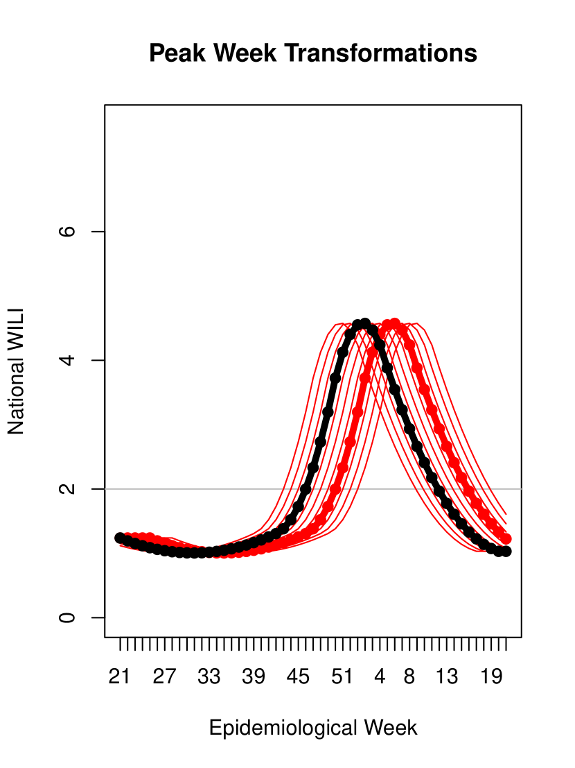
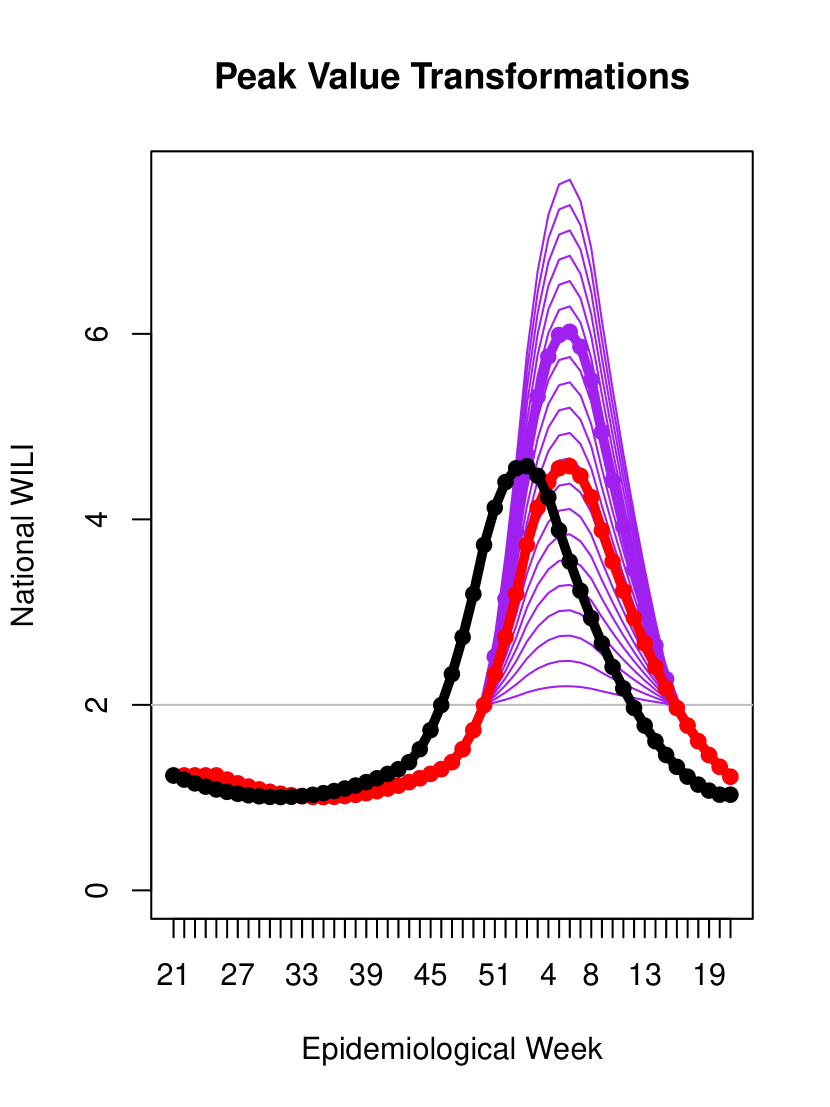
We model the underlying curve ${f^{{s_{\mathrm{curr}}}}}$ for the current season as the curve generated by a randomly sampled parameter configuration $\left\langle f,\sigma,\nu,\theta,\mu\right\rangle$ , using the following equation:

{f^{{s_{\mathrm{curr}}}}}(i)=b+\frac{\theta-b}{\max_{j}f(j)-b}\left[f\left(\frac{i-\mu}{\nu}+\operatorname*{arg\,max}_{j}f(j)\right)-b\right],

where $b$ is the current year’s baseline wILI level (i.e., the onset threshold) for the selected geographical region, e.g., $2\%$ for the U.S. as a nation for the 2013–2014 flu season. Figure 2 illustrates the peak week and peak height transformations.

The data model for the current season’s wILI values ${y^{{s_{\mathrm{curr}}}}}$ is the same as that for historical seasons, shown in Equation 1.

4.2.3 Sampling from the posterior

We use importance sampling [28] to obtain a large set of curves from the posterior weighted by how closely they match the epidemic curve so far, beginning with week 40. More concretely, we obtain a single weighted sample from the posterior by (i) sampling a historical smoothed curve $f$ , noise level $\sigma$ , and transformation parameters $\nu$ , $\theta$ , and $\mu$ from the prior; (ii) applying the peak height, peak week, and pacing transformations; (iii) assigning the curve an “importance weight” or “likelihood” based on how well it matches existing observations for the current seasons; and (iv) drawing noisy wILI observations around the curve for the rest of the season. We apply this procedure many times to obtain a collection of possible wILI trajectories and associated weights, forming a probability distribution over possible futures for the current season.

4.2.4 Forecasting targets

For the CDC challenge, we were interested in four forecasting targets of interest to policy makers: the epidemic’s onset, peak week, peak, and duration.

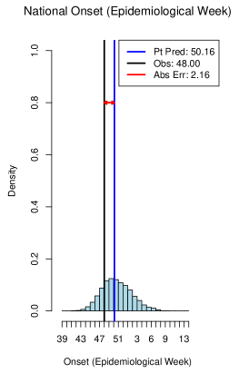
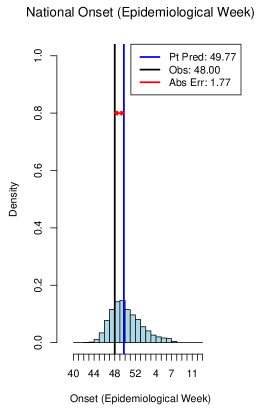
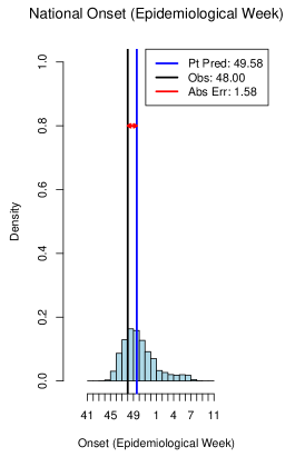
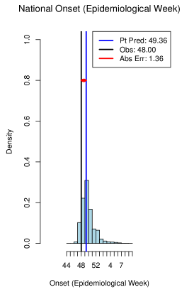
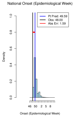
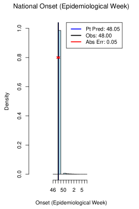
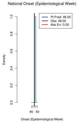
Onset:: The first week that the wILI curve is above a specified CDC baseline wILI level, and remains there for at least the next two weeks. For example, the 2013–2014 national baseline wILI level was $2\%$ , so the onset was the first in at least three consecutive weeks with wILI levels above $2\%$ .
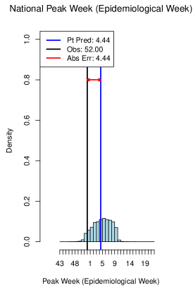
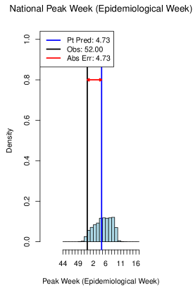
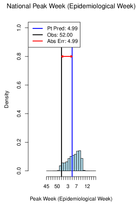
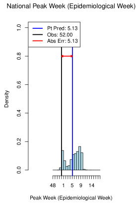
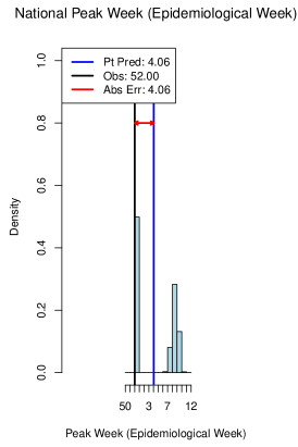
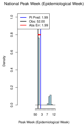
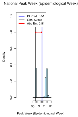
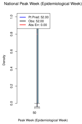
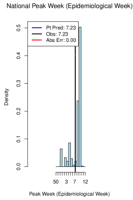
Peak Week:: The week in which the wILI curve attains its maximum value.
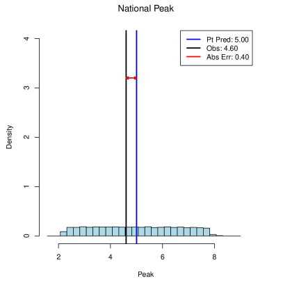
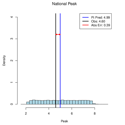
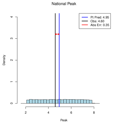
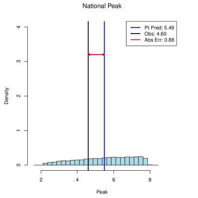
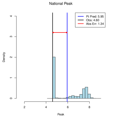
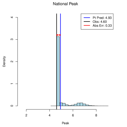
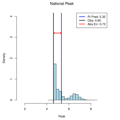
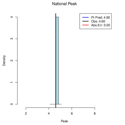
Peak:: The maximum observed wILI value in a season.
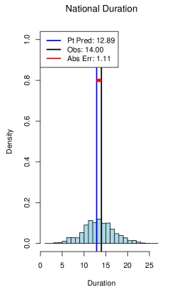
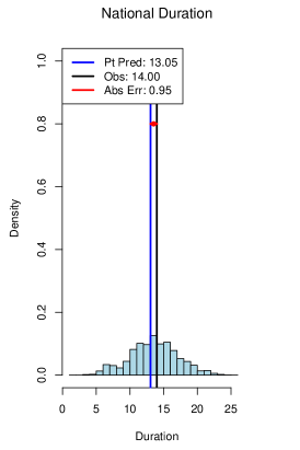
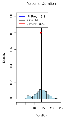
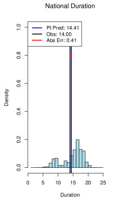
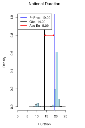
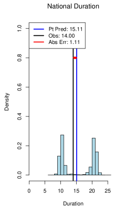
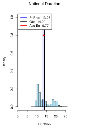
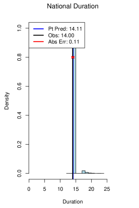
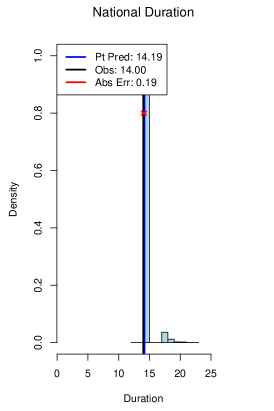
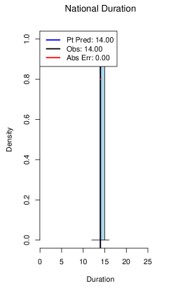
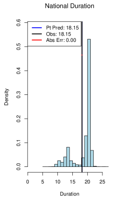
Duration:: Roughly, how many weeks the wILI level remained above the CDC baseline since the onset. We defined this more rigorously as the sum of the lengths of all periods of three or more consecutive weeks with wILI levels above the CDC baseline.

We generate distributions for each of these targets by repeatedly (i) sampling a possible wILI trajectory and associated weight from the posterior, (ii) calculating the four forecasting targets for that trajectory,⁴⁴4 When calculating the forecasting targets for a particular wILI trajectory, we use the observed wILI values when they are available. This ensures that the framework will not consider target values that seem impossible with the currently available data, e.g., peak height values lower than the currently observed maximum. Future data revisions may make some of these previously “impossible” values valid again, though. and (iii) storing these four values along with the trajectory’s weight. We represent these forecasting target posterior distributions with histograms, and generate point estimates by taking the posterior mean for each target. Figure 3 illustrates the links between the elements of the framework.

Figure 3: Diagram of the prior and posterior model. Shaded nodes, unobserved quantities; shaded dashed nodes, proprietary data; unshaded nodes, publicly available data; thin arrows, dependencies; thick arrows, deterministic dependencies; textual annotations, descriptions of how we incorporate dependencies.

4.2.5 Incorporating non-final and digital data

At the time that forecasts were generated, GFT estimates were available for the current week and previous week, while ILINet wILI measurements were available only for times further in the past. We produced one set of forecasts using the latest ILINet data by itself, and another that incorporated GFT data. We considered two methods of including GFT data: (i) using GFT estimates only for the two weeks in which ILINet data was not yet available, and (ii) also using GFT estimates in place of recent ILINet values which may be revised significantly in the future. Since GFT attempts to minimize RMSE on the logit scale [21], we performed linear regression to reduce the RMSE on the non-logit scale that our framework works with.

5 Results

5.1 Predictions for the 2013–2014 season

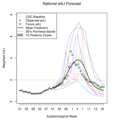
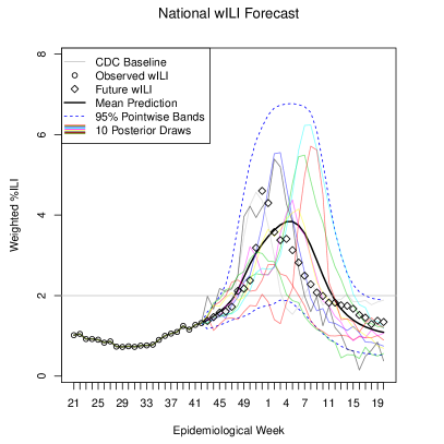
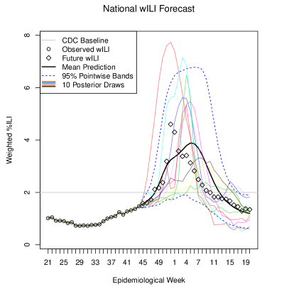
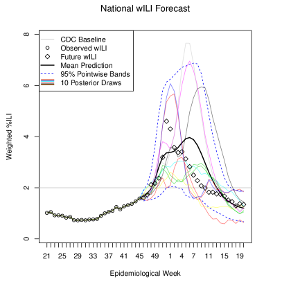
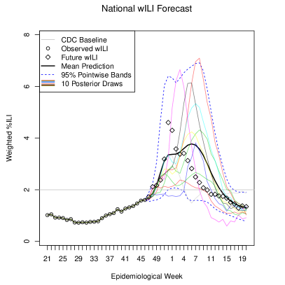
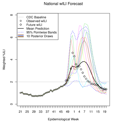
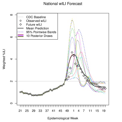
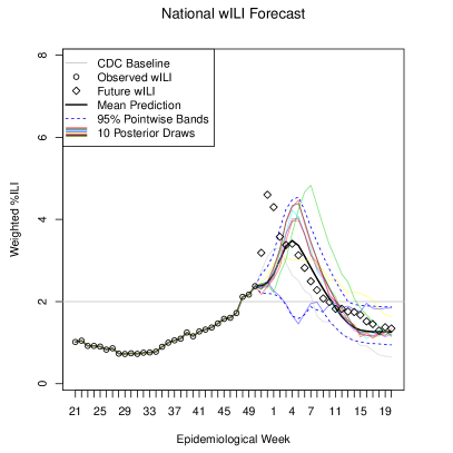
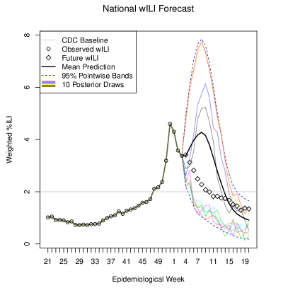
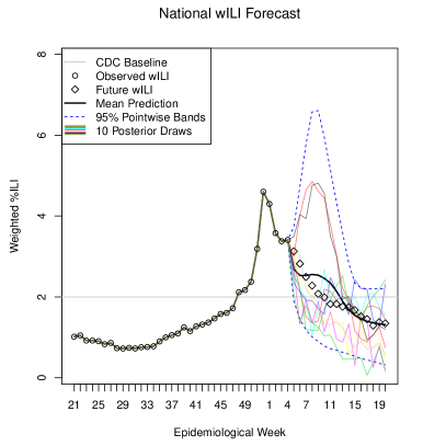
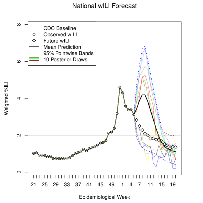
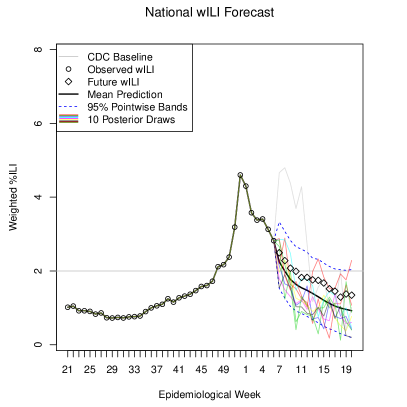
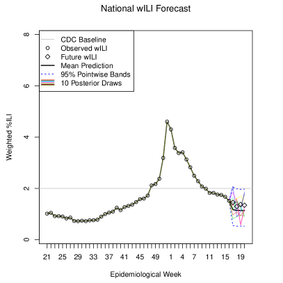
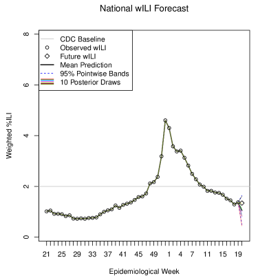
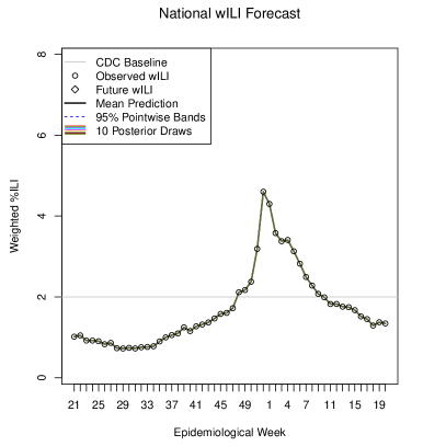
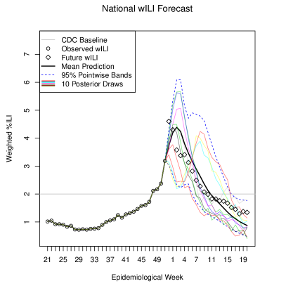
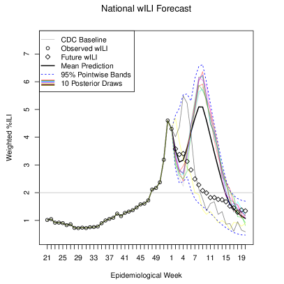
For the CDC challenge, we generated biweekly forecasts from December 5 (epidemiological week 49) to March 27 (week 9), for the nation as a whole, and individually for each the 10 HHS regions. Included below is a summary of our current framework’s forecasts throughout the season, based on revised data and no GFT. We display 10 draws from the posterior representing likely wILI curves, as well as the posterior mean and $5$ th and $95$ th posterior percentiles for the wILI value for each week. The posterior provides a histogram for each of the four forecasting targets; we report the mean target value as a point prediction.

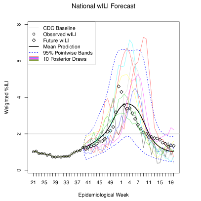
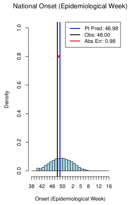
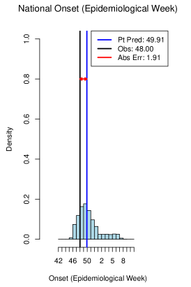
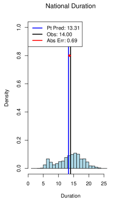
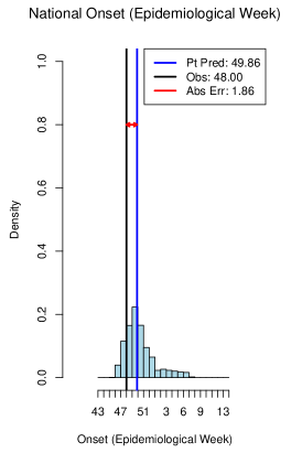
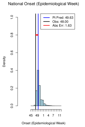
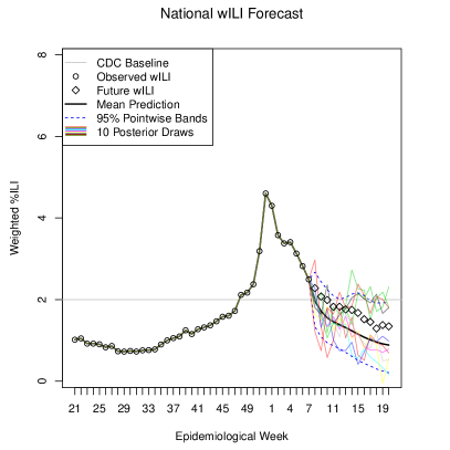
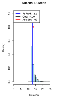
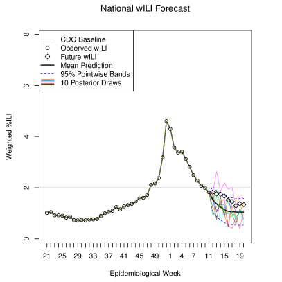
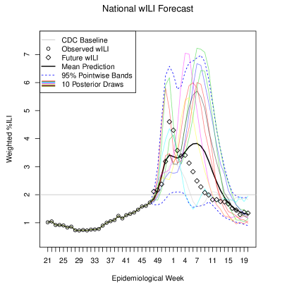
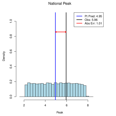
5.1.1 Week 49 (December 5) forecast, using wILI data through week 47

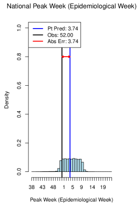
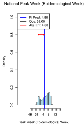
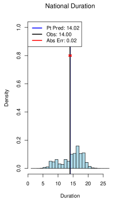
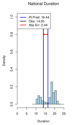
During the week of the first forecast, all of the available wILI values are below the CDC onset threshold. Predictions for the onset, as shown in Figure 4, are concentrated near the actual value, and the error in the point prediction is fairly small. Much of this error can be attributed to the sudden jump in wILI at the onset, which corresponds to Thanksgiving week. The number of patients seen per reporting provider in ILINet drops noticeably on Thanksgiving week and even more significantly during winter holidays; at these times, there is a systematic bias towards higher wILI values. The forecasts for the overall wILI curves and the other three targets contain much more uncertainty, as shown by wider histograms that more closely resemble the prior distribution. The peak of the epidemic could potentially occur early or late, and be mild or strong.

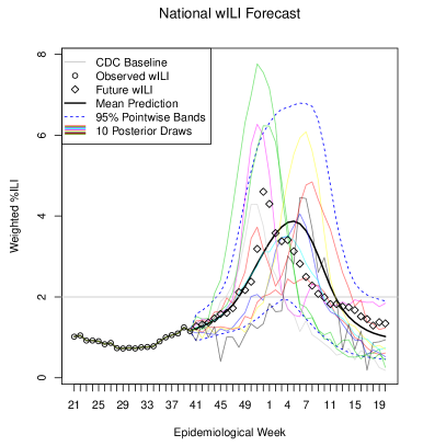
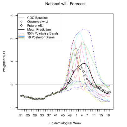
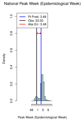
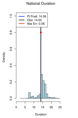
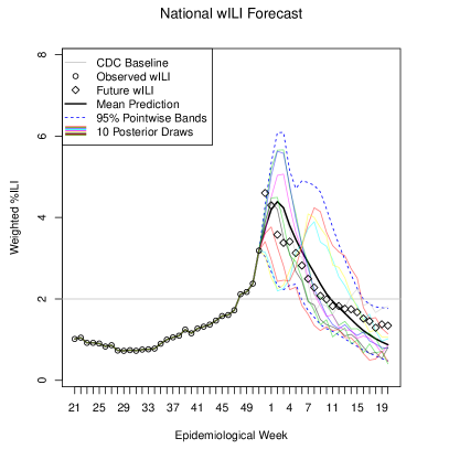
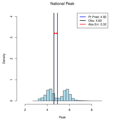
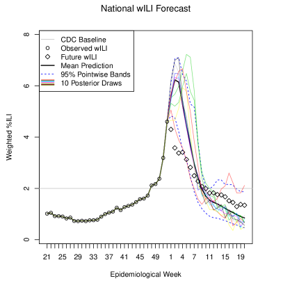
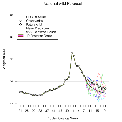
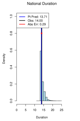
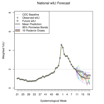
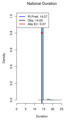
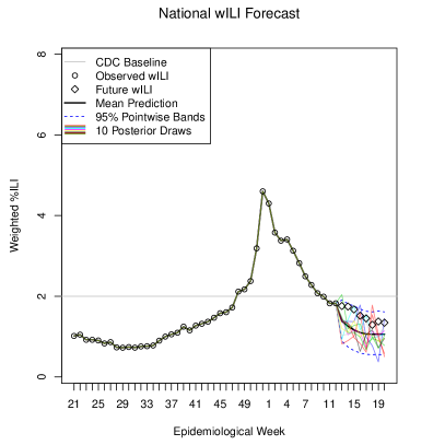
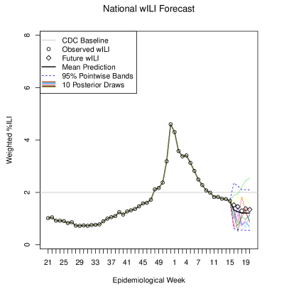
5.1.2 Week 1 (January 2) forecast, using wILI data through week 51

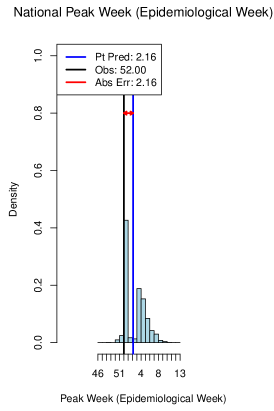
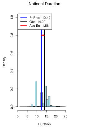
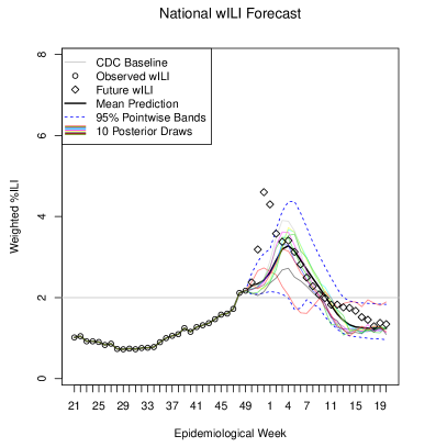
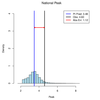
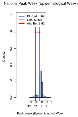
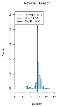
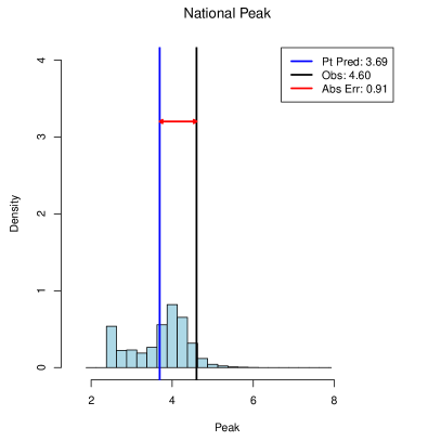
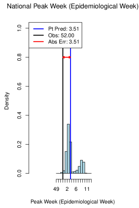
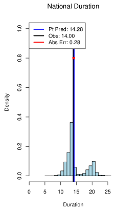
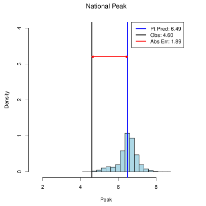
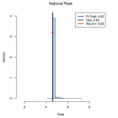
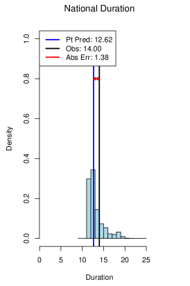
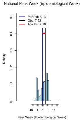
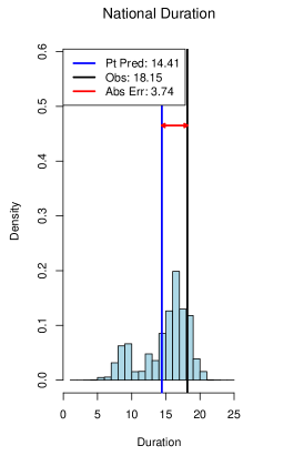
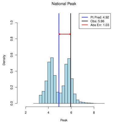
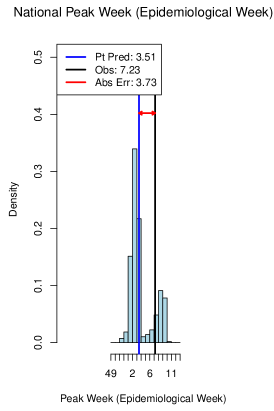
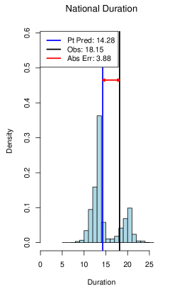
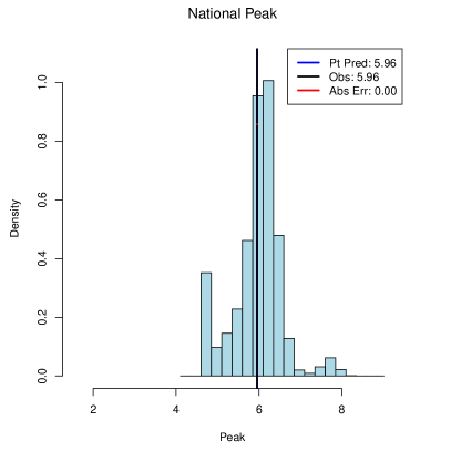
Figure 5 shows that, with data available up to the week before the sudden peak, the framework matches the observed wILI trajectory fairly closely with many of the posterior draws. The sudden peak can be explained as a combination of elevated ILI-related visits combined with a relative decrease in unrelated visits associated with winter holidays. The framework selects posterior curves with slightly later peaks of similar height, as well as seasons with much later peaks, which contain secondary peaks around the winter holidays. The onset has already been confirmed, so its histogram is a point mass. Duration predictions narrow around the actual duration.

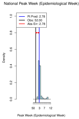
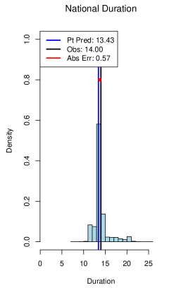
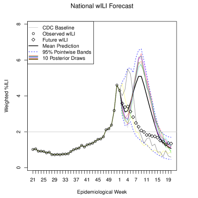
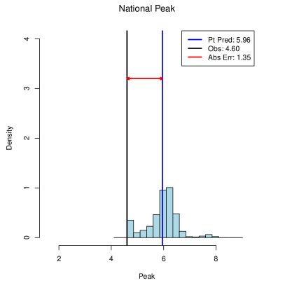
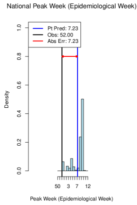
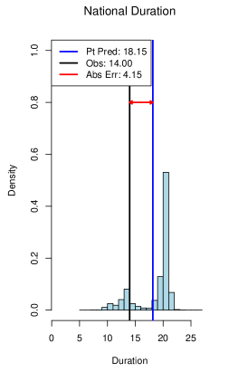
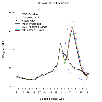
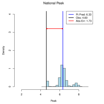
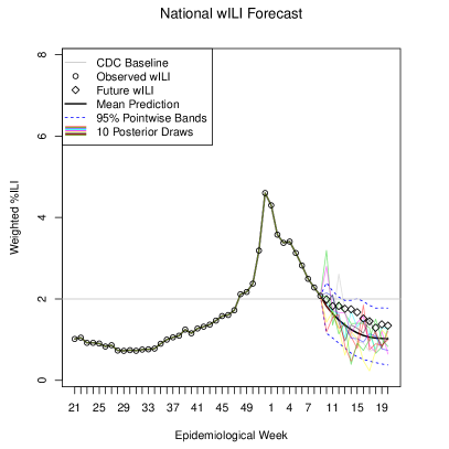
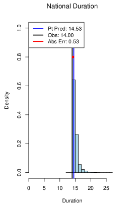
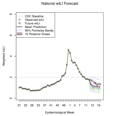
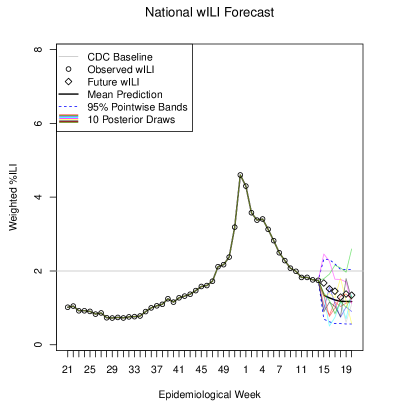
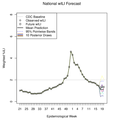
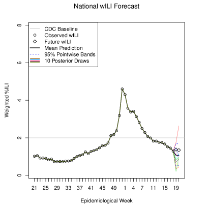
5.1.3 Week 3 (January 16) forecast, using wILI data through week 1

Figure 6 shows that, after the sudden peak, the posterior for the 2013–2014 epidemic contained primarily transformed versions of the 2006–2007 curve, which featured a relatively large secondary peak around winter holidays, followed by a primary peak in early February. This tendency to “latch” onto a particular shape is one of the reasons why transformed versions of curves were used instead of just the curves themselves. Given the limited amount of historical wILI data available, including transformations provides a larger number of reasonable curves from which to pick. However, the latching phenomenon still occurs, and degrades performance in this forecast.

Subsequent forecasts continue to predict another, later, primary or secondary peak, until some time late in the season, in which forecasts match the falling tail of the epidemic curve.

8.1 contains forecasts like those referenced above for the entire 2013–2014 season.

5.2 Point prediction trends

Figure 7 shows the observed forecasting target values for the 2013–2014 season, and predictions over time for the current framework, older versions used to generate submissions with different transformations and curve weighting methods, and Epicast, a system used to collect and aggregate human-generated predictions.

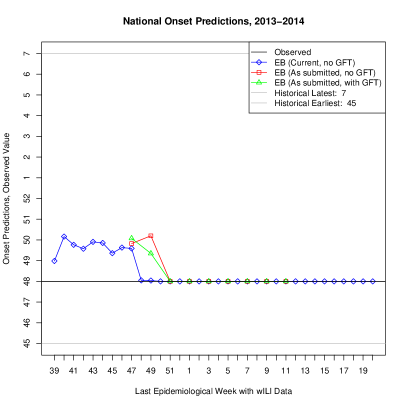
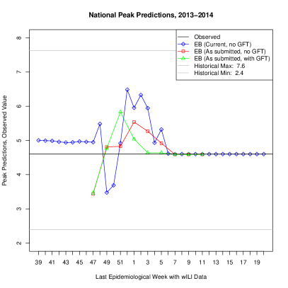
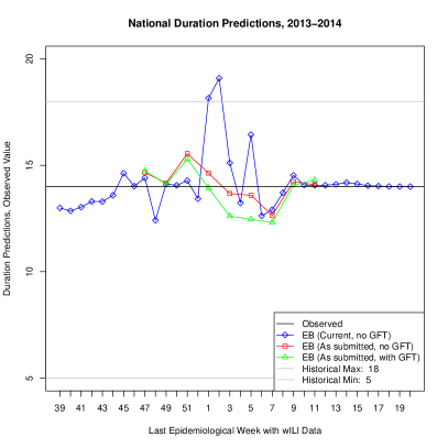
The small error in the onset before it occurred, as well as the underestimation of the peak in weeks 49 and 50, can be attributed to not factoring in holiday effects; at least some of these effects are smoothed out by the trend filtering process, or shifted to different times and heights by the peak week and height transformations. Later errors in the peak week, peak, and duration result from latching onto transformed versions of one or two past epidemic curves with two peaks. Including additional curves in the prior, improving selection of transformations, accounting for holiday effects, and incorporating additional types of data may help increase performance in this case. However, when considering these types of changes, we must be careful not to select modifications only to give good performance only on the 2013–2014 season; that would be fitting, rather than prediction. The ideal way to compare different approaches would be to analyze the error of true, prospective forecasts over many seasons; however, this comes at the prohibitive cost of waiting through these seasons. Instead, we prefer to use cross-validated error when predicting past seasons rather than performance on a single season.

5.3 Estimated average error from cross-validation

We used leave-one-out cross-validation to approximate the average error in the framework’s forecasting target point predictions as a function of the epidemiological week of the last wILI observation used. For each historical season ${s_{\mathrm{cv}}}$ , we produced forecasts using the rest of the historical seasons to build the prior, and recorded the average error of our point predictions across these 15 seasons for each week in the flu season. While this approach allows later seasons to be used while predicting earlier seasons, this should not introduce too much bias because the framework treats the different seasons as if they were independent. The advantage of including these later seasons is that each one uses $14$ epidemic curves to build its prior, and should give a better idea of what to expect when making forecasts with a similar number of “past” seasons. Another detail to note is that these error estimates were generated using the final revision of the wILI data, and do not include any effects from approximating the most recent wILI values from the tentative values available in real-time.

Figures 8, 9, 10, and 11 show the cross-validated error for our current empirical Bayes framework, as well a few other approaches, for each for the four forecasting targets. The methods for predicting ${\mathrm{tar}_{j}}({y^{{s_{\mathrm{cv}}}}})$ are summarized below.

Baseline (Mean of Other Seasons):: takes the average target value across the 14 other seasons, completely ignoring any data from the current season.
Pinned Baseline (Mean of Other Seasons, Conditioned on Current Season to Date):: constructs 14 possible wILI trajectories for the current season by using the available observations for previous weeks and other historical curves for future weeks; reports the mean target value across these 14 trajectories.
Pointwise Percentile [29]:: Constructs a single possible future wILI trajectory using the pointwise $q$ th quantile from other seasons; estimates an appropriate value of $q$ from the observed data so far.
$k$ Nearest Neighbors:: Uses a method similar to existing systems for shorter-term prediction [18] to identify $k$ sections of other seasons’ data that best match recent observations, and uses them to construct and weight $k$ possible future wILI trajectories.
Empirical Bayes (Transformed Versions of Other Seasons’ Curves):: Our current framework, using transformed versions of other seasons’ curves to form the prior.
Empirical Bayes (SIR Curves):: Our current framework, using scaled and shifted SIR curves rather than other seasons’ curves to form the prior.

From the graphs, we see that the empirical Bayes framework gives competitive or lower mean absolute error in forecasting target point predictions than the best of the other baselines consistently across many prediction weeks. An important advantage of this approach over many of the other baselines is that it provides a smooth distribution over possible curves and target values, rather than just a single point. From this distribution, we can calculate point predictions to minimize some expected type of error or loss, build credible intervals, and make probabilistic statements about future wILI and target values.

6 Discussion

We developed an empirical Bayes approach to forecasting epidemic curves and targets, and applied it to wILI estimates to generate predictions for the 2013–2014 influenza season as part of a CDC challenge. Our method’s forecasts for the season were reasonable to the human eye, and cross-validated error estimates indicate that it competes with or improves upon results from various baseline predictors. This method generates a distribution over future wILI curves and forecasting targets, rather than just point predictions. The framework does not require or rely on mechanistic models, which often will not match well with observed data, but instead generates possible epidemic curves from past history with a few reasonable transformations.

A potential downside is that we also gain no insight into the process underlying the epidemic. Since it is nonmechanistic, our framework can be easily applied to other epidemic curves. We have already used it to predict dengue incidence in the 2014 World Cup game cities with little modification [29], and expect that application to additional diseases will require little adjustment, and could be considered as a baseline for other, more specialized, predictors. It should be possible to make important decisions, such as what transformations to use, automatically by minimizing cross-validated prediction error on historical data.

We are investigating many ways to improve our approach’s performance. Better ways of incorporating non-final wILI and other surveillance data, complemented by short-term predictors such as regression, should improve whole-season predictions as well. Our current framework only uses ILINet and GFT, but can include additional sources of data such as Twitter activity, thermometer sales, and lab testing data. Modeling and adjusting for holiday effects in each data source may also improve accuracy. For now, we have treated regional epidemics as independent, but have found spatial correlations in historical data; shrinking forecasts together based on proximity may improve our results.

7 Acknowledgments

We thank Matt Biggerstaff, Lyn Finelli, and the CDC for organizing the challenge and the followup workshop, and for helpful discussions regarding influenza surveillance in the U.S.

Research reported in this publication was supported by the National Institute Of General Medical Sciences of the National Institutes of Health under Award Number U54 GM088491. The content is solely the responsibility of the authors and does not necessarily represent the official views of the National Institutes of Health. This material is based upon work supported by the National Science Foundation Graduate Research Fellowship Program under Grant No. DGE-1252522. Any opinions, findings, and conclusions or recommendations expressed in this material are those of the authors and do not necessarily reflect the views of the National Science Foundation. DF was a predoctoral trainee supported by NIH T32 training grant T32 EB009403 as part of the HHMI-NIBIB Interfaces Initiative.

References

[1] Molinari NAM, Ortega-Sanchez IR, Messonnier ML, Thompson WW, Wortley PM, et al. (2007) The annual impact of seasonal influenza in the US: measuring disease burden and costs. Vaccine 25: 5086–5096.
[2] Laporte RE (1993) How to improve monitoring and forecasting of disease patterns. BMJ: British Medical Journal 307: 1573–1574.
[3] Hethcote HW (2000) The mathematics of infectious diseases. SIAM review 42: 599–653.
[4] Ferguson NM, Cummings DA, Fraser C, Cajka JC, Cooley PC, et al. (2006) Strategies for mitigating an influenza pandemic. Nature 442: 448–452.
[5] Colizza V, Barrat A, Barthelemy M, Valleron AJ, Vespignani A (2007) Modeling the worldwide spread of pandemic influenza: baseline case and containment interventions. PLoS Medicine 4: e13.
[6] Bansal S, Pourbohloul B, Meyers LA (2006) A comparative analysis of influenza vaccination programs. PLoS Medicine 3: e387.
[7] Lee BY, Brown ST, Cooley P, Potter MA, Wheaton WD, et al. (2010) Simulating school closure strategies to mitigate an influenza epidemic. Journal of Public Health Management and Practice: JPHMP 16: 252.
[8] Grefenstette JJ, Brown ST, Rosenfeld R, DePasse J, Stone NT, et al. (2013) FRED (A Framework for Reconstructing Epidemic Dynamics): an open-source software system for modeling infectious diseases and control strategies using census-based populations. BMC Public Health 13: 940.
[9] Dugas AF, Jalalpour M, Gel Y, Levin S, Torcaso F, et al. (2013) Influenza forecasting with Google Flu Trends. PLoS ONE 8: e56176.
[10] Chretien JP, George D, Shaman J, Chitale RA, McKenzie FE (2014) Influenza forecasting in human populations: a scoping review. PLoS ONE 9: e94130.
[11] Nsoesie EO, Brownstein JS, Ramakrishnan N, Marathe MV (2014) A systematic review of studies on forecasting the dynamics of influenza outbreaks. Influenza and Other Respiratory Viruses 8: 309–16.
[12] Shaman J, Karspeck A (2012) Forecasting seasonal outbreaks of influenza. Proceedings of the National Academy of Sciences of the United States of America 109: 20425–30.
[13] Ong JBS, Chen MIC, Cook AR, Lee HC, Lee VJ, et al. (2010) Real-time epidemic monitoring and forecasting of H1N1-2009 using influenza-like illness from general practice and family doctor clinics in Singapore. PLoS ONE 5: e10036.
[14] Goldstein E, Cobey S, Takahashi S, Miller JC, Lipsitch M (2011) Predicting the epidemic sizes of influenza A/H1N1, A/H3N2, and B: a statistical method. PLoS Medicine 8: e1001051.
[15] Vergu E, Grais RF, Sarter H, Fagot JP, Lambert B, et al. (2006) Medication sales and syndromic surveillance, France. Emerging Infectious Diseases 12: 416–21.
[16] Soebiyanto RP, Adimi F, Kiang RK (2010) Modeling and predicting seasonal influenza transmission in warm regions using climatological parameters. PLoS ONE 5: e9450.
[17] Polgreen PM, Nelson FD, Neumann GR (2007) Use of prediction markets to forecast infectious disease activity. Clinical infectious diseases: an official publication of the Infectious Diseases Society of America 44: 272–9.
[18] Viboud C, Boëlle PY, Carrat F, Valleron AJ, Flahault A (2003) Prediction of the spread of influenza epidemics by the method of analogues. American Journal of Epidemiology 158: 996–1006.
[19] Brammer L, Budd AP, Finelli L (2013) Seasonal and pandemic influenza surveillance, John Wiley & Sons Ltd, chapter 12. pp. 200–210. doi:10.1002/9781118543504.ch16. URL http://dx.doi.org/10.1002/9781118543504.ch16.
[20] Centers for Disease Control and Prevention (2013). Overview of influenza surveillance in the United States. URL http://www.cdc.gov/flu/weekly/overview.htm. [Online; accessed 29-August-2014].
[21] Ginsberg J, Mohebbi MH, Patel RS, Brammer L, Smolinski MS, et al. (2009) Detecting influenza epidemics using search engine query data. Nature 457: 1012–4.
[22] Cook S, Conrad C, Fowlkes AL, Mohebbi MH (2011) Assessing Google flu trends performance in the United States during the 2009 influenza virus A (H1N1) pandemic. PLoS ONE 6: e23610.
[23] Copeland P, Romano R, Zhang T, Hecht G, Zigmond D, et al. (2013) Google Disease Trends: An update. Nature 457: 1012–1014.
[24] Lazer D, Kennedy R, King G, Vespignani A (2014) Big data. The parable of Google Flu: traps in big data analysis. Science (New York, NY) 343: 1203–5.
[25] Santillana M, Zhang DW, Althouse BM, Ayers JW (2014) What can digital disease detection learn from (an external revision to) Google Flu Trends? American Journal of Preventive Medicine 47: 341–347.
[26] Lamb A, Paul MJ, Dredze M (2013) Separating Fact from Fear: Tracking Flu Infections on Twitter. In: HLT-NAACL. pp. 789–795.
[27] Tibshirani RJ, et al. (2014) Adaptive piecewise polynomial estimation via trend filtering. The Annals of Statistics 42: 285–323.
[28] Liu JS (2008) Monte Carlo strategies in scientific computing. Springer.
[29] van Panhuis WG, Hyun S, Blaney K, Marques Jr ET, Coelho GE, et al. (2014) Risk of dengue for tourists and teams during the world cup 2014 in brazil. PLoS Neglected Tropical Diseases 8: e3063.