Magnetoresistance in multilayer fullerene spin valves: a first-principles study

Abstract

Carbon-based molecular semiconductors are explored for application in spintronics because their small spin-orbit coupling promises long spin life times. We calculate the electronic transport from first principles through spin valves comprising bi- and tri-layers of the fullerene molecules C₆₀ and C₇₀, sandwiched between two Fe electrodes. The spin polarization of the current, and the magnetoresistance depend sensitively on the interactions at the interfaces between the molecules and the metal surfaces. They are much less affected by the thickness of the molecular layers. A high current polarization ($\mathrm{CP}>90$%) and magnetoresistance ($\mathrm{MR}>100$%) at small bias can be attained using C₇₀ layers. In contrast, the current polarization and the magnetoresistance at small bias are vanishingly small for C₆₀ layers. Exploiting a generalized Jullière model we can trace the differences in spin-dependent transport between C₆₀ and C₇₀ layers to differences between the molecule-metal interface states. These states also allow one to interpret the current polarization and the magnetoresistance as a function of the applied bias voltage.

I Introduction

Spintronics focuses on information processing with charge carrier spins.Fert (2008) Developments in spintronics, such as giant magnetoresistance (GMR) and tunneling magnetoresistance (TMR) in metallic spin valves have revolutionized the fields of magnetic recording and storage. Novel devices are envisioned that use injection and manipulation of spin-polarized currents in semiconductors, such as the spin transistor.Zutic et al. (2004) Molecular semiconductors (MSC), i.e., semiconductors comprised of organic molecules, have caught the attention because carbon-based molecules promise to have advantages over conventional semiconductors such as Si or GaAs.Tombros et al. (2007); Dediu et al. (2009) The relatively weak spin-orbit coupling and hyperfine interactions in such molecules lead to long spin life times, i.e., long spin relaxation and dephasing times, which would allow for robust spin operations and read-out. The use of molecules also opens up a route towards single molecule spintronics, where individual molecules are considered for electronic functions. Indeed, magnetoresistance effects have been demonstrated at the single molecule level.Schmaus et al. (2011); Kawahara et al. (2012); miyamachi et al. (2012); Yoshida et al. (2013)

Many experimental studies deal with vertical spin valves, where molecular layers are sandwiched between two ferromagnetic metal (FM) electrodes, and are used either as a tunnel barrier, or as charge and spin transport medium. Large magnetoresistance (MR) effects have been reported in spin valves based upon layers of organic molecules such as tris(8-hydroxy-quinolinato)-aluminium (Alq₃),Xiong et al. (2004); Santos et al. (2007); Dediu et al. (2008); Schoonus et al. (2009); Sun et al. (2010); Barraud et al. (2010); Schulz et al. (2011) or fullerenes such as C₆₀.Gobbi et al. (2011); Tran et al. (2012); Zhang et al. (2013, 2014); Li et al. (2014) Similar effects have been observed in zinc methyl phenalenyl (ZMP) layers sandwiched between a FM electrode and a non-magnetic electrode, where the spin valve effect has been attributed to the special characteristics of the molecule/FM interface layer.Raman et al. (2013) In phenomenological models for the observed spin transport effects the electronic structure, in particular the spin-polarization, of the MSC/FM interfaces plays a pivotal role in spin injection into the MSC.Barraud et al. (2010) This has prompted the suggestion that highly spin-polarized currents in spintronic devices may be obtained by exploiting such interface interactions, which has been dubbed “spinterface science”,Sanvito (2010) and has motivated research into the role played by the interfaces.Cinchetti et al. (2008); Chan et al. (2010); Lach et al. (2012); Steil et al. (2013); Dediu (2013); Droghetti et al. (2014); Shi et al. (2014)

The electronic structure of metal-organic interfaces is accessible through first-principles calculations, and can in some cases be interpreted using simple models for the energy level line-up at interfaces.Giovannetti et al. (2008); Rusu et al. (2010); Bokdam et al. (2011) Photoemission spectroscopy or scanning tunnelling microscopy, combined with first-principles calculations, enable a detailed analysis of the spin-dependent electronic properties of metal-organic interfaces. Bonding between a molecule and a ferromagnetic metal leads to spin-split (anti)bonding states and induces a spin polarization that extends onto the molecule.Atodiresei et al. (2010); Brede et al. (2010); Javaid et al. (2010); Tran et al. (2011); Kawahara et al. (2012); Schwöbel et al. (2012); Tran et al. (2013); Djeghloul et al. (2013) For instance, calculations on C${}_{60}|$Fe(001) interfaces yield a magnetic moment of 0.2 $\mu_{B}$ induced on the C₆₀ molecules.Tran et al. (2013) For electronic transport in spintronics devices, not the overall spin-polarization is decisive however, but the spin-polarization of the states around the Fermi energy.

First-principles transport calculations might establish the connection between such molecule-metal interface states and MR effects in molecular spin valves. Calculations have been applied to model currents through a single molecule attached to two FM metal electrodes,Rocha et al. (2005); Ning et al. (2008); Koleini and Brandbyge (2012); Liang et al. (2012); Bagrets et al. (2012) as they can be realized in STM experiments, for instance, where MR effects have been demonstrated at the single molecule level.Schmaus et al. (2011); Kawahara et al. (2012); miyamachi et al. (2012); Yoshida et al. (2013) A single molecule is however not a good starting-point for modeling transport through MSCs, as binding a molecule to two electrodes markedly changes its electronic structure. For instance, fullerene molecules attached to two Fe electrodes result in metallic conduction,whereas fullerene multilayers give a small, tunneling conductance.Tran et al. (2012)

We have calculated the spin-dependent transport through multilayer graphene spin valves,Karpan et al. (2007, 2008) and recently have demonstrated the feasibility of such calculations on molecular spin valves.Çakır et al. (2014) In this paper we expand the scope of such calculations. In particular we focus on Fe$|$fullerene$|$Fe spin valves with bi- and tri-layers of C₆₀ and C₇₀ fullerene molecules. Fullerenes are particularly interesting molecules for applications in spintronics due to the absence of hydrogen atoms that lead to spin dephasing via hyperfine interactions. The Fe(001) surface is a well-established substrate for organic spintronics allowing for a controlled growth of fullerene layers.Tran et al. (2011, 2013) We study the links between the spin-dependent transport through these fullerene multilayers, and the electronic structure of the metal-organic interfaces by first-principles transport calculations. A generalized Jullière or factorization model, defined in Sec. II, serves to rationalize these links, in particular when a single molecular state dominates the transport.

The set-up of the transport calculations is discussed in Sec. III, and the results are discussed in Sec. IV. Somewhat surprisingly, there is a qualitative diference between the spin transport through C₆₀ and C₇₀ layers, which can be traced to a difference in the molecule-metal interface states. In particular, adsorption of C₇₀ leads to a spin-polarized interface state very close to the Fermi level that gives rise to a large current polarization (CP) and MR. In contrast, the corresponding interface state associated with adsorption of C₆₀ lies further from the Fermi level. That state is accessible by increasing the bias voltage over the spin valve, which however only leads to a relatively moderate CP and MR. Sec. V summarizes the main conclusions.

II Theory

Following Landauer, the current through a quantum conductor $I^{\sigma}$ at finite bias $V$ and zero temperature, carried by independent particles with spin $\sigma=\uparrow,\downarrow$, is given byDatta (1995)

$$I^{\sigma}=\frac{e}{h}\sum_{\sigma}\int_{E_{F}-\frac{1}{2}eV}^{E_{F}+\frac{1}{2}eV}T^{\sigma}(E,V)dE,$$ (1)

with $T^{\sigma}$ the transmission probability of an electron with spin $\sigma$. Expressed in non-equilibrium Green’s functions (NEGF)Caroli et al. (1971); Brandbyge et al. (2002)

$$T^{\sigma}=\mathrm{Tr}\left[\bm{\Gamma}^{\sigma}_{R}\mathbf{G}_{RL}^{\sigma,r}\bm{\Gamma}^{\sigma}_{L}\mathbf{G}_{LR}^{\sigma,a}\right],$$ (2)

where $\mathbf{G}_{RL}^{\sigma,r}$ is the block of the retarded Green’s function matrix connecting the right and left leads through the quantum conductor, $\bm{G}_{LR}^{\sigma,a}=\left(\mathbf{G}_{RL}^{\sigma,r}\right)^{\dagger}$ is the corresponding advanced Green’s function matrix block, and $\mathbf{\bm{\Gamma}}^{\sigma}_{R(L)}=-2\mathrm{Im}\bm{\Sigma}^{\sigma}_{R(L)}$, with $\bm{\Sigma}^{\sigma}_{R(L)}$ the self-energy matrix connecting the quantum conductor to the ideal right (left) lead.Datta (1995); Brandbyge et al. (2002); Khomyakov et al. (2005)

One can rewrite this expression by formally partitioning the system in to a right and a left part and a coupling between the parts. A natural partitioning for organic spin valves is a left and a right interface, each consisting of a molecular layer adsorbed on a metal surface.Çakır et al. (2014) Any molecular layers between the two interfaces are then incorporated in the coupling Hamiltonian.

In the tunneling regime, where the effects of multiple reflections between left and right parts can be neglected, it is possible to simplify the transmission to

$$T^{\sigma}=\mathrm{4\pi^{2}}\sum_{i,j}n_{Ri}^{\sigma}n_{Lj}^{\sigma}\left|H_{Ri,Lj}^{\sigma}\right|^{2},$$ (3)

see Appendix A. Here $n^{\sigma}_{Ri}$ and $n^{\sigma}_{Lj}$ are the spectral densities corresponding to states $i$ and $j$ of the right and left part, respectively.Datta (1995); Mahan (1990) The matrices $\mathbf{H}^{\sigma}_{RL}=\left(\mathbf{H}^{\sigma}_{LR}\right)^{\dagger}$ represent the coupling between the right and left parts.

Equation (3) can be used as a starting point to derive a generalized Jullière expression for the magnetoresistance of an organic spin valve. If the magnetization of the right electrode is reversed when switching from parallel (P) to anti-parallel (AP) configuration, it is reasonable to expect that the spectral densities of majority and minority spins are interchanged, but not altered,

$$(n_{Ri}^{\sigma})_{AP}\approx(n_{Ri}^{-\sigma})_{P}.$$ (4)

Following a simple tight-binding argument, the coupling matrix elements in the tunneling regime scale with the overlap between the wave functions of the left and right parts, which roughly scales as the product of these functions. If this is the case, then a decent approximation for the coupling matrix elements in the AP case should be

$$\left|H_{Ri,Lj}^{\sigma}\right|^{2}_{AP}\approx\left|H_{Ri,Lj}^{\sigma}H_{Ri,Lj}^{-\sigma}\right|_{P}.$$ (5)

Using Eqs. (4) and (5) one can express the normalized difference $\Delta_{P/AP}=(T_{P}-T_{AP})/(T_{P}+T_{AP})$ between the transmissions $T=\sum_{\sigma}T^{\sigma}$ in the P and AP cases as

$$\Delta_{P/AP}=\frac{\sum_{i,j}\left(\nu_{Ri,Lj}^{\uparrow}-\nu_{Ri,Lj}^{\downarrow}\right)\left(\nu_{Lj,Ri}^{\uparrow}-\nu_{Lj,Ri}^{\downarrow}\right)}{\sum_{i,j}\left(\nu_{Ri,Lj}^{\uparrow}+\nu_{Ri,Lj}^{\downarrow}\right)\left(\nu_{Lj,Ri}^{\uparrow}+\nu_{Lj,Ri}^{\downarrow}\right)},$$ (6)

in terms of the weighted densities

$$\nu_{Ri,Lj}^{\sigma}=n_{Ri}^{\sigma}\left|H_{Ri,Lj}^{\sigma}\right|;\;\nu_{Lj,Ri}^{\sigma}=n_{Lj}^{\sigma}\left|H_{Ri,Lj}^{\sigma}\right|,$$ (7)

which are calculated for the P case. Equation (6) has the form of a generalized Jullière expression in terms of weighted spin-polarization densities.Jullière (1975)

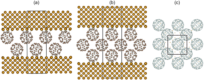
Figure 1: (color online) (a),(b) side views of the bilayer and trilayer C₆₀ junctions, Fe$|($C${}_{60})_{n}|$Fe, $n=2,3$; (c) top view of interlayer C₆₀ stacking. The black lines denote the supercell used.

The expression can be simplified if the spectral density of each spin is dominated by a single state. For adsorbed molecules this is likely to be the case for an energy range close to one particular molecular level, the HOMO or LUMO, for instance. The sum $\sum_{i,j}$ in Eq. (6) is then over one state, giving $\Delta_{P/AP}=P_{R}P_{L}$ with $P_{R}=(\nu^{\uparrow}_{R,L}-\nu^{\downarrow}_{R,L})/(\nu^{\uparrow}_{R,L}+\nu^{\downarrow}_{R,L})$ the weighted spin-polarization density of the right interface, where $\nu^{\sigma}_{R,L}=n^{\sigma}_{R}|H^{\sigma}_{RL}|$, and $P_{L}$ a similar expression for the spin-polarization density of the left interface. In linear response, where the bias $V$ in Eq. (1) is infinitesimal, only the transmissions at the Fermi energy are important. The magnetoresistance then becomes $\mathrm{MR}=(T_{AP}-T_{P})/T_{AP}=2P_{L}P_{R}/(1-P_{L}P_{R})$, which has the appearance of a Jullière expression.Jullière (1975)

Assuming that a single state is dominant also allows for simplifying the transmission of Eq. (3) to $T^{\sigma}=\mathrm{4\pi^{2}}n_{R}^{\sigma}n_{L}^{\sigma}\left|H_{RL}^{\sigma}\right|^{2}$. For a symmetric junction in the P configuration at zero bias, one has $n_{L}^{\sigma}=n_{R}^{\sigma}$, and thus $\sqrt{T_{P}^{\sigma}}=n_{R}^{\sigma}|H^{\sigma}_{RL}|$, linking the transmission directly to the interface density of states $n_{R}$. Applying a bias voltage $V$ across a tunnel barrier, it is reasonable to assume that the small transmission current does not change the charge distribution. The spectral densities of the right and left interfaces can then be obtained from rigid shifts of the corresponding densities at zero bias, $n^{\sigma}_{Ri}(E,V)=n^{\sigma}_{Ri}(E-eV/2,0)$ and $n^{\sigma}_{Lj}(E,V)=n^{\sigma}_{Lj}(E+eV/2,0)$. Again assuming that at each energy a single state is dominant (not necessarily the same state at all energies), it then follows

$$T_{P}^{\sigma}\left(E,V\right)\approx\sqrt{T_{P}^{\sigma}\left(E-\frac{eV}{2},0\right)}\sqrt{T_{P}^{\sigma}\left(E+\frac{eV}{2},0\right)},$$ (8)

and

$$T_{AP}^{\sigma}\left(E,V\right)\approx\sqrt{T_{P}^{\sigma}\left(E-\frac{eV}{2},0\right)}\sqrt{T_{P}^{-\sigma}\left(E+\frac{eV}{2},0\right)}.$$ (9)

With these expressions one can interpret the transmission spectra at any bias, starting from the spectrum of the P case at zero bias.

III Computational Details

We optimize the structures of the Fe(001)$|$fullerene interfaces within density functional theory (DFT), using projector augmented waves (PAW),Blöchl (1994); Kresse and Joubert (1999) as implemented in the Vienna Ab initio Simulation Package (VASP).Kresse and Hafner (1993); Kresse and Furthmüller (1996) All plane waves up to a kinetic energy cutoff of 400 eV are included in the basis set. The spin-polarized PBE functional is used to describe exchange and correlation.Perdew et al. (1996) As the bonding between the Fe surface and the fullerene molecules is strong, including van der Waals interactions is not necessary. An equidistant $k$-point grid with a spacing of 0.02 Å^-1 is used for the Brillouin zone sampling. Structures are assumed to be relaxed when the difference of the total energies between two consecutive ionic steps is less than 10^-5 eV and the maximum force on each atom is less than 0.01 eV/Å.

Electronic transport in Fe$|$fullerene$|$Fe junctions is calculated using the self-consistent NEGF technique, Eqs. (1) and (2), as implemented in TranSIESTA.Soler et al. (2002); Brandbyge et al. (2002) We employ Troullier-Martins (TM) normconserving pseudo-potentials (NCPP),Troullier and Martins (1991) the PBE functional, and an energy cutoff for the real-space mesh of 200 Ry. Numerical orbital basis sets are used, comprising single-$\zeta$ and double-$\zeta$ plus polarization for Fe and C, respectively. To compare the VASP and SIESTA results, we benchmark the calculations on the magnetic properties of bulk bcc Fe and the clean Fe(001) surface, see Appendix B.

The Fe(001)$|$fullerene interfaces are modeled by a $4\times 4$ Fe(001) surface unit cell, with a cell parameter of 11.32 Å, containing one fullerene molecule, see Fig. 1. For comparison, the nearest neighbor distance in C₆₀ and C₇₀ crystals is 10-11 Å.Heiney et al. (1991); van Smaalen et al. (1994) From a number of possible adsorption geometries, we have identified the most stable structures of adsorbed C₆₀ and C₇₀ molecules. Details can be found in Appendix B.

A structure for a bilayer-C₆₀ junction, Fe$|($C${}_{60})_{2}|$Fe, is generated by mirroring the optimized Fe(001)$|$C₆₀ interface structure, and translating it in plane by half a lattice constant, such that the packing C₆₀ molecules in the bilayer resembles that of the (001) orientation of the fcc C₆₀ crystal, see Fig. 1. The spacing between the C₆₀ layers is chosen such that the shortest intermolecular C–C distance is 3.2 Å, which is a typical value for close-packed fullerenes or carbon nanotubes. Along the same lines a structure for a trilayer C₆₀ junction, Fe$|($C${}_{60})_{3}|$Fe, is generated, as well as structures for bi- and trilayer C₇₀ junctions, Fe$|($C${}_{70})_{n}|$Fe, $n=2,3$.

Using a 6$\times$6 in-plane $k$-point mesh in the $4\times 4$ Fe(001) supercell suffices to obtain converged results for the transmission, as is demonstrated by Fig. 2.

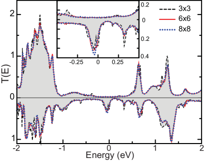
Figure 2: (color online) Transmissions $T^{\uparrow}_{P}(E)$ of majority (top) and $T^{\downarrow}_{P}(E)$ (bottom) of minority spin channels of Fe$|$(C${}_{70})_{2}|$Fe at zero bias. The Fermi level is at zero energy. Curves are given for $3\times 3$, $6\times 6$, and $8\times 8$ $k$-point grid samplings.

IV Results and discussion

IV.1 Linear Response

The conductance in the linear response regime is determined by the transmission at the Fermi level. Table 1 gives the calculated transmissions of bilayers and trilayers of C₆₀ and C₇₀ molecules, sandwiched between two Fe(001) electrodes, with magnetizations parallel (P), or anti-parallel (AP). The transmission through a trilayer is up to two orders of magnitude smaller than the transmission through a bilayer. In absolute numbers the transmission through a bilayer is fairly high; the small numbers obtained for a trilayer are typical for the tunneling regime. The sizeable difference in the transmissions of bi- and tri-layers shows that we are not in the regime of resonant transmission though a molecular level.

The transmissions of C₇₀ bi- or tri-layer are consistently higher than that of their C₆₀ counterparts, although the relevant energy levels and wave functions (HOMO and LUMO) of the isolated C₆₀ and C₇₀ molecules are not so different. Below we will argue that the difference in transmission is caused by differences in the states formed at the Fe/molecule interfaces.

Table 1: Transmissions $T^{\uparrow(\downarrow)}_{P}$ of majority (minority) spins through Fe$|$layer$|$Fe at zero bias, magnetizations of electrodes parallel; transmission $T_{AP}^{\uparrow(\downarrow)}$, magnetizations anti-parallel; current polarization CP $=(T^{\uparrow}_{P}-T^{\downarrow}_{P})/(T^{\uparrow}_{P}+T^{\downarrow}_{P})$, normalized magnetoresistance $\Delta_{P/AP}=(T_{P}-T_{AP})/(T_{P}+T_{AP})$, and optimistic magnetoresistance MR $=(T_{P}-T_{AP})/T_{AP}$ (in %).

layer	$T_{P}^{\uparrow}(E_{F})$	$T_{P}^{\downarrow}$	$T_{AP}^{\uparrow(\downarrow)}$	$\sqrt{T_{P}^{\uparrow}T_{P}^{\downarrow}}$	CP	$\Delta_{P/AP}$	MR
(C60)2	$8.6(-3)$	$8.4(-3)$	$9.1(-3)$	$8.5(-3)$	1.3	$-3.6$	$-6.9$
(C60)3	$2.1(-4)$	$2.9(-4)$	$2.5(-4)$	$2.5(-4)$	$-16$	$1.1$	$2.2$
(C70)2	$2.3(-2)$	$1.9(-1)$	$6.3(-2)$	$6.6(-2)$	$-78$	$25$	$67$
(C70)3	$2.9(-4)$	$4.1(-3)$	$9.6(-4)$	$11.0(-4)$	$-87$	$42$	$144$

The most prominent difference between C₆₀ and C₇₀ molecules is in the spin polarization of the transmission. Whereas for C₆₀ layers the transmissions of majority and minority spins are almost equal, for C₇₀ layers the transmission of minority spin is approximately an order of magnitude larger than that of majority spin. It means that the current polarization in linear response, $\mathrm{CP}=(T^{\uparrow}_{P}-T^{\downarrow}_{P})/(T^{\uparrow}_{P}+T^{\downarrow}_{P})$, of C₆₀ junctions at low bias is small, $|\mathrm{CP}|<20$%. In contrast, the CP of C₇₀ junctions is very substantial, $|\mathrm{CP}|=80$-$90$%. Moreover the magnetoresistance $\mathrm{MR}=(T_{P}-T_{AP})/T_{AP}$ is large for C₇₀ junctions, exceeding 100% for trilayers, whereas the MR for C₆₀ junctions is vanishingly small. The differences between the CP and MR of C₆₀ and C₇₀ junctions have the same origin, as we will see below.

In the following we interpret the behavior of C₆₀ and C₇₀ junctions using the model outlined in Sec. II. If a single channel dominates the transmission and the junction is symmetric, then transmission can be factorized according to Eqs. (8) and (9), and the factors $\sqrt{T_{P}^{\sigma}}=n_{R}^{\sigma}|H^{\sigma}_{RL}|$, are weighted interface density of states. Figure 3(a) shows $\sqrt{T_{P}^{\sigma}(E)}$, derived from the transmission spectra of a bilayer C₆₀ junction. For comparison, Fig. 3(b) shows the density of states of a C₆₀/Fe(001) interface, projected on the molecule (PDOS), see Appendix B. There is indeed a striking resemblance between the transmission spectra and the PDOSs.

The peaks in the PDOS can be labeled according to their molecular character. As the molecule-substrate interaction is large, these peaks correspond to hybrid interface states, which are significantly broadened in energy compared to the pure molecular states. Moreover, the interface states are exchange-split because the substrate is ferromagnetic. Nevertheless the dominant components of their molecular contributions can still be identified; details can be found in Appendix B.

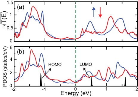
Figure 3: (color online) (a) $\sqrt{T_{P}^{\uparrow}(E)}$ for majority spin (blue) and $\sqrt{T_{P}^{\downarrow}(E)}$ for minority spin (red) at zero bias for Fe$|$C₆₀-C${}_{60}|$Fe junction; (b) projected density of states (PDOS) of the Fe$|$C₆₀ interface.

The Fermi level is situated in a gap in the transmission spectra of the bilayer C₆₀ junction, which according to the PDOS and the molecular level spectrum corresponds to the HOMO-LUMO gap. One has $T_{P}^{\uparrow}(E_{F})\approx T_{P}^{\downarrow}(E_{F})$, and this absence of spin polarization is also observed in the PDOS. It is then not surprising to find that $\mathrm{CP}\approx 0$ and $\mathrm{MR}\approx 0$ at low bias. The two small peaks in the minority spin transmission $T_{P}^{\downarrow}(E)$ at $E\approx E_{F}\pm 0.2$ eV will give rise to a moderate nonzero CP and MR at finite bias, as we will see in the next section. These peaks are derived from hybridyzing the Fe(001) surface states with the C₆₀ LUMO.

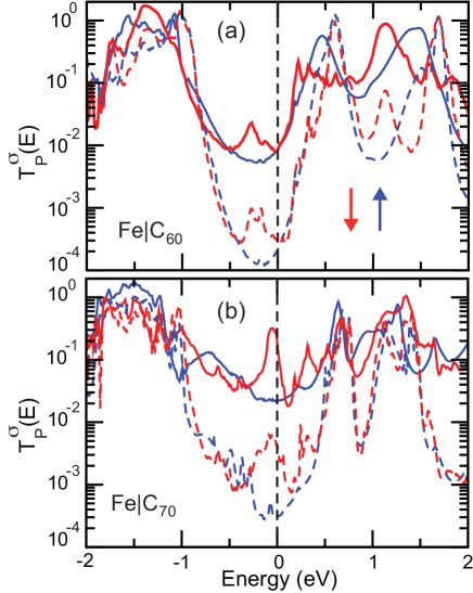
Figure 4: (color online) (a) Calculated transmission spectra $T_{P}^{\sigma}(E)$ of majority (blue) and minority (red) spins of bilayer C₆₀ (solid lines) and trilayer C₆₀ (dashed lines) junctions. The Fermi level $E_{F}$ is at zero energy. (b) Calculated transmission spectra of C₇₀ junctions.

Figure 4 gives the transmission spectra $T_{P}^{\sigma}(E)$ of all the multilayers studied in this paper. The peaks in the transmission spectra of order unity correlate with resonant transmission through molecular levels. In the bilayer case the latter are strongly hybridized with the Fe surface, resulting in broad peaks. The transmission spectra for bi- and tri-layers are qualitatively similar, but for the trilayer the peaks in the transmission are considerably sharper. For the trilayer transmission of order unity can only be achieved via resonant transmission through the molecular levels of the middle layer.

The transmission for energies in the gaps between the peaks imply tunneling through the molecular layers. In all cases the Fermi level is situated in the gap in the transmission spectrum corresponding to the molecular HOMO-LUMO gap. The transmission for energies inside this gap is higher for C₇₀ layers than for C₆₀ layers. This is consistent with the difference between these molecules regarding the spatial extent of their interface states. The interaction between C₇₀ and the Fe(001) surface gives interface states that are more delocalized over the molecules, see Appendix B. Such a delocalization effectively leads to thinner tunnel barriers.

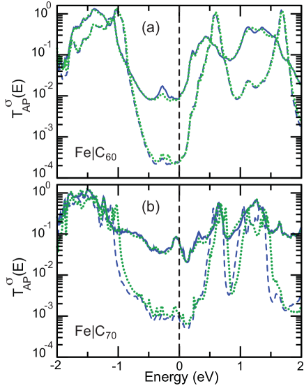
Figure 5: (color online) Calculated transmission spectra $T_{AP}^{\sigma}(E)$ (blue) of bilayer (solid lines) and trilayer (dashed lines) molecular junctions of (a) C₆₀ and (b) C₇₀.foo The Fermi level $E_{F}$ is at zero energy. The green dotted lines give the factorization approximation $2\sqrt{T_{P}^{\sigma}(E)T_{P}^{-\sigma}(E)}$, see Eq. (9).

The most prominent difference between C₆₀ and C₇₀ in the transmission close to the Fermi level is a peak in the minority spin channel, compare Figs. 4(a) and (b). For C₇₀ a prominent peak in the transmission is situated very close to the Fermi level, whereas for C₆₀ a smaller peak lies at $\sim 0.2$ eV below the Fermi level. Both these peaks can be traced to an interface state derived from the molecular LUMO, created by the adsorption of the molecules on the surface. Differences in the bonding of the two molecules to the Fe(001) surface give a different energy for this state, which has a major effect on the spin transport properties of the molecular layers, see Table 1. For C₇₀ this minority spin state at the Fermi level is at the origin of a large CP and a large MR, whereas for C₆₀ the fact that this state is not exactly at the Fermi level results in a small CP and a small MR. Going from two to three layers the transmission in the HOMO-LUMO gap decreases, but the overall pattern of the transmission remains the same.

Figure 5 shows the transmission spectra $T_{AP}^{\sigma}(E)$ calculated with the magnetizations of the two Fe electrodes in anti-parallel configurations. Also shown are the results of the factorization approximation, Eq. (9), with $V=0$. Following the discussion in Sec. II this approximation is designed for the tunneling regime, when multiple reflections are absent, and when a single channel dominates the transmission. The results shown in Fig. 5 seem to indicate that the factorization approximation has a somewhat wider applicability, and also works reasonably well if the transmission is larger than is typical for tunneling. From the factorization approximation it becomes clear that the CP and the MR are related properties. If the CP is large (small), then the MR is large (small).

There are of course situations where the factorization approximation fails. For instance it always give a $\mathrm{MR}\geq 0$ for a symmetric junction in the linear response regime. This is easy to see from the discussion following Eqs. (6) and (7). In a symmetric junction at zero bias, the weighted spin-polarizations of left and right interfaces is identical, $P_{R}=P_{L}$, which implies that $\Delta_{P/AP}\geq 0$ and $\mathrm{MR}\geq 0$. The small negative MR at zero bias calculated for a bilayer C₆₀ junction in Table 1 is clearly in disagreement with this. By construction this junction is symmetric, and the right Fe(001)$|$C₆₀ interface is identical to the left interface.

Nevertheless it is possible to obtain a negative MR, even for a symmetric junction. To obtain $\Delta_{P/AP}<0$ in Eq. (6), giving $\mathrm{MR}<0$, (at least) two molecular states at each interface should be involved. In absence of any off-diagonal coupling, i.e., $H_{Ri,Lj}^{\sigma}=0$; $i\neq j$, this would still give $\Delta_{P/AP}\geq 0$, so in order to obtain a negative sign one needs a significant off-diagonal coupling. Suppose for simplicity that $H_{Ri,Lj}^{\sigma}=h$; $i\neq j$, and $H_{Ri,Li}^{\sigma}=0$, then in a system with two states it suffices to have $n_{1}^{\downarrow}>n_{1}^{\uparrow}$ and $n_{2}^{\downarrow}<n_{2}^{\uparrow}$ to obtain $\Delta_{P/AP}<0$. In other words, a negative MR in a symmetric junction can be obtained if a strong coupling between two states exists, where one of the states has a dominant majority spin character at the Fermi level, and the other one has a dominant minority spin character.

As in the bilayer C₆₀ junction the Fermi level falls between peaks in the transmission spectra and in the PDOS, see Fig. 3, it is quite likely that the tails of more than one molecular state are involved at this energy. The fact that in the trilayer C₆₀ junction the negative MR disappears shows that the coupling between these states across the junction is crucial. Despite its limitations, the factorization model can be very helpful in interpreting spin transport properties as we will see in the next section.

IV.2 Finite bias

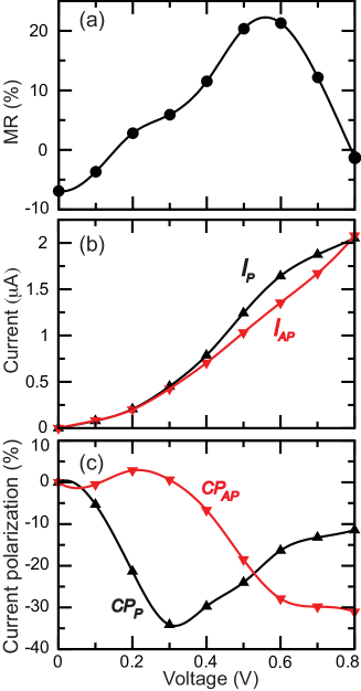
Figure 6: (color online) (a) Magneto-resistance $\mathrm{MR}=(I_{P}-I_{AP})/I_{AP}$ of the C₆₀ bilayer junction as function of bias $V$. (b) Total currents $I_{P}$ (black) and $I_{AP}$ (red) for the magnetizations of both electrodes parallel, respectively anti-parallel. (c) Current polarization $\mathrm{CP}=(I^{\uparrow}-I^{\downarrow})/(I^{\uparrow}+I^{\downarrow})$.

Figure 6(a) shows the magneto-resistance (MR) as a function of the applied bias $V$, calculated self-consistently for the Fe$|$bilayer C${}_{60}|$Fe junction. Over the voltage range studied the MR increases from $-7$% at $V=0$ to $+21$% at $V=0.6$ V, before dropping again to $-1$% at $V=0.8$ V. The calculated total currents $I_{P}$ and $I_{AP}$ as a function of the applied bias $V$ are shown in Fig. 6(b). The currents are distinctly non-linear, and the junction is non-ohmic. The transmissions of the bilayer C₆₀ junction at energies in the interval $E_{F}\pm 0.5$ eV are of order $10^{-2}$, see Figs. 4(a) and 5(a), which, although much smaller than unity, is still larger than is typical for a tunnel junction. In other words, a bilayer C₆₀ junction is still quite a leaky junction.

Figure 6(c) shows the spin polarization of the current or current polarization (CP). At zero bias, $V=0$, the total current $I_{P}=I^{\uparrow}+I^{\downarrow}$ through a parallel junction is not polarized, i.e., $I^{\uparrow}=I^{\downarrow}$. Upon increasing the bias the minority spin-current becomes dominant, $I^{\downarrow}>I^{\uparrow}$, and the total current $I_{P}$ becomes polarized with a minimum of $-35$% at $V=0.3$ V. Remarkably, a current polarization of a similar magnitude can be achieved in an AP junction, albeit at a bias that is more than twice as large.

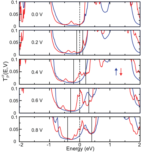
Figure 7: (color online) $T_{P}^{\uparrow}(E,V)$ for majority spin (blue) and $T_{P}^{\downarrow}(E,V)$ for minority spin (red) of the C₆₀ bilayer junction as function of bias, from top to bottom: $V=0.0$, 0.2, 0.4, 0.6, 0.8 V. The vertical lines enclose the energy interval over which to integrate to obtain the total current according to Eq. (1).

Figure 7 shows the transmission spectra $T_{P}^{\sigma}(E,V)$ at finite bias, calculated self-consistently, for a range of different biases. The factorization model allows one to interpret the trends in these spectra, and in the MR and the CP. According to Eq. (8) one can construct the transmission at finite bias starting by multiplying a pair of $\sqrt{T_{P}^{\sigma}}$ spectra, displaced by $\pm eV/2$, cf. Fig. 3. At zero bias the CP is zero, reflecting the fact that $T_{P}^{\uparrow}(E_{F},0)=T_{P}^{\downarrow}(E_{F},0)$. Close to the Fermi level at $E\approx E_{F}\pm 0.2$ eV, the minority spin transmission $T_{P}^{\downarrow}(E,0)$ show two small peaks, Fig. 3(a). Both these peaks are derived from interface states involving the C₆₀ LUMO, as discussed in Appendix B.

Increasing the bias means that these two peaks move towards one another, according to Eq. (8). If one displaces the $T_{P}^{\downarrow}(E,0)$ spectra by $\pm 0.2$ eV, these two peaks coincide at the same energy. According to Eq. (8) such a displacement corresponds to a bias of 0.4 V. As the majority spin transmission $T_{P}^{\uparrow}(E,0)$ does not have peaks in this energy region, it means that at this bias the CP is negative, which indeed is the case, as can be seen in Fig. 6(c). Upon increasing the bias further, peaks in the majority spin transmission also move into the integration window for the total current. This means that the CP decreases with increasing bias, which can also be observed Fig. 6(c).

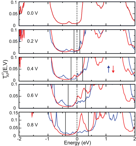
Figure 8: (color online) $T_{AP}^{\uparrow}(E,V)$ for majority spin (blue) and $T_{AP}^{\downarrow}(E,V)$ for minority spin (red) of the C₆₀ bilayer junction as function of bias, from top to bottom: $V=0.0$, 0.2, 0.4, 0.6, 0.8 V. The vertical lines enclose the energy interval over which to integrate to obtain the total current according to Eq. (1).

To explain the CP for the AP case one must realize that the role of majority and minority spin are now interchanged for one of the electrodes. Within the factorization model, one has to multiply a $\sqrt{T_{P}^{\sigma}}$ curve with a $\sqrt{T_{P}^{-\sigma}}$ curve, displaced by $\pm eV/2$, see Fig. 3. The first peak in $T_{P}^{\uparrow}$ is at $E\approx E_{F}+0.5$ eV. In order to have that coincide with the peak in $T_{P}^{\downarrow}$ at $E\approx E_{F}-0.2$ eV, it requires a bias $V\approx 0.7$ V. Multiplying the $\sqrt{T_{P}^{\sigma}}$ and $\sqrt{T_{P}^{-\sigma}}$ factors then gives a peak in the transmission spectrum $T_{AP}^{\downarrow}(E,V)$ at $E=0,V=0.7$ V. Indeed the self-consistent transmission spectrum $T_{AP}^{\sigma}$ at finite bias, given in Fig. 8, shows this peak in $T_{AP}^{\downarrow}$ growing with increasing bias. Therefore, for the AP case one expects to see a zero CP at low bias, and a decreasing CP at higher bias, which is indeed the case in Fig. 6(c).

The behavior of the MR in Fig. 6(a) can be interpreted qualitatively along the same lines. The MR is zero at zero bias because the transmission of both spin channels is almost the same. Upon increasing the bias foremost the transmission of the minority spin channel in the P case increases, cf. Fig. 7, which according to the factorization model originates from shifting the two minority spin peaks at $E\approx E_{F}\pm 0.2$ eV closer together, see Fig. 3(a), as discussed above. There is not such an increase in the AP case, as the roles of majority and minority spin in one of the electrodes are reversed. This means that, upon increasing the bias, $I_{AP}<I_{P}$ as can be observed in Fig. 6(b). Upon further increase of the bias the transmission of the minority spin channel in the AP case increases, cf. Fig. 8, as the minority spin peak at $E\approx E_{F}-0.2$ eV starts to approach the majority spin peak at $E\approx E_{F}+0.5$ eV, as discussed in the previous paragraph. It means that at a higher bias $I_{AP}$ increases relative to $I_{P}$, and the MR decreases again, see Fig. 6(a).

The behavior of the Fe(001)$|$bilayer C${}_{70}|$ junction as a function of bias voltage has been explained in Ref. Çakır et al., 2014. It is much simpler than that of the bilayer C₆₀ junction. At zero bias a peak in the transmission for minority spin is found very close to the Fermi level, which results in a substantial CP and MR at zero bias. Upon increasing the bias this peak decreases as in the factorization model the two factors are displaced from one another, cf. Eq. (9). That results in a monotonic derease of both $|\mathrm{CP}|$ and $|\mathrm{MR}|$ as a function of bias.

The transmission spectra of the molecular trilayer junctions are qualitatively similar to those of their corresponding bilayers, see Figs. 4 and 5. This means that as a function of bias one expects the CP and the MR of trilayers to behave similarly to their bilayer counterparts. Of course the absolute currents for the trilayer cases will be much lower than for the bilayer cases. The fact that the general behavior of the CP and the MR does not depend critically on the thickness of the molecular layers illustrates the central role played by the metal-molecule interfaces.

V Summary and Conclusions

We calculate the electronic transport from first principles through spin valves composed of bilayers and trilayers of the fullerene molecules C₆₀ and C₇₀, sandwiched between two ferromagnetic Fe electrodes. Despite the similarity of the two molecules, they give rise to a markedly different behavior of their spin-dependent currents. C₇₀ bi- and tri-layers give large negative current polarizations of $-80$ to $-90$% at small bias, where the minus sign indicates that the currents are dominated by minority spin. In contrast, the current polarization generated by C₆₀ layers is zero at small bias. Similarly, the magnetoresistance of C₇₀ spin valves at small bias is $70$ to $140$%, whereas that of C₆₀ spin valves is only a few percent. As a function of applied bias across the spin valve, the current polarization of C₇₀ junctions increases monotonically toward zero, and the magnetoresistance decreases toward zero. For bilayer C₆₀ spin valves the current polarization goes through a minimum of $-35$% at $V=0.3$ V, as a function of applied bias, and the magnetoresistance goes through a maximum of $24$% at $V=0.55$ V.

All these trends can be explained using a generalized Jullière or factorization model, which couples the spin-dependent transport of the junctions to the electronic structure of the molecule-metal interfaces. The favorable properties of C₇₀ junctions can be traced to an interface state in the minority spin, which is derived from the molecular LUMO, and lies very close the Fermi energy. Although a similar state also exists for C₆₀, it lies $\sim 0.2$ eV below the Fermi level, which means that it becomes accessible only at a higher bias voltage. The binding of the molecules to the surface plays a decisive role in determining the position of these states with respect to the Fermi level. Increasing the thickness of the molecular layers decreases the abolute value of the currents, but it has a relative small effect on the sizes of the current polarization and of the magnetoresistance, which stresses the pivotal role played by the molecule-metal interfaces.

Appendix A Partitioning

To calculate the transmission, Eq. (2), one needs the block of the Green’s function matrix $\mathbf{G}_{RL}$ connecting the right and left leads via the quantum conductor, where we omit the spin index for the moment to simplify the notation. We partition the system in to a left and a right part,

$$\left(\begin{array}[]{cc}\mathbf{G}_{LL}&\mathbf{G}_{LR}\\ \mathbf{G}_{RL}&\mathbf{G}_{RR}\end{array}\right)\left(\begin{array}[]{cc}E\mathbf{I}_{L}-\mathbf{H}_{LL}&-\mathbf{H}_{LR}\\ -\mathbf{H}_{RL}&E\mathbf{I}_{R}-\mathbf{H}_{RR}\end{array}\right)=\left(\begin{array}[]{cc}\mathbf{I}_{L}&0\\ 0&\mathbf{I}_{R}\end{array}\right),$$ (10)

where the diagonal blocks $\mathbf{H}_{LL}$ and $\mathbf{H}_{RR}$ of the Hamiltonian matrix represent the semi-infinite left and right parts, and the off-diagonal blocks $\mathbf{H}_{RL}=\left(\mathbf{H}_{LR}\right)^{\dagger}$ represent the coupling between the right and left parts.

Formally solving Eq. (10) then gives for the off-diagonal block of the Green’s function matrix

$$\mathbf{G}_{RL}=\mathbf{g}_{R}\mathbf{H}_{RL}\left(\mathbf{I}_{L}-\mathbf{g}_{L}\mathbf{H}_{LR}\mathbf{g}_{R}\mathbf{H}_{RL}\right)^{-1}\mathbf{g}_{L},$$ (11)

with

$$\mathbf{g}_{R}=\left(E\mathbf{I}_{R}-\mathbf{H}_{RR}\right)^{-1};\;\mathbf{g}_{L}=\left(E\mathbf{I}_{L}-\mathbf{H}_{LL}\right)^{-1},$$ (12)

the Green’s function matrices of the uncoupled right and left parts. Expression (11) can be used to rewrite Eq. (2). Moreover it is easy to show that $\mathbf{g}_{R(L)}^{a}\mathbf{\bm{\Gamma}}_{R(L)}\mathbf{g}_{R(L)}^{r}=2\pi\mathbf{n}_{R(L)}$, where $\mathbf{n}_{R(L)}=-\pi^{-1}\mathrm{Im}\mathbf{g}_{R(L)}^{r}$ is the spectral density matrix of the right (left) part.Datta (1995); Mahan (1990) Equation (2) then becomes

$$T=\mathrm{4\pi^{2}Tr}\biggl{[}\mathbf{n}_{R}\mathbf{H}_{RL}\bigl{(}\mathbf{I}_{L} - \mathbf{g}_{L}^{r}\mathbf{H}_{LR}\mathbf{g}_{R}^{r}\mathbf{H}_{RL}\bigr{)}^{-1}$$

$$\mathbf{n}_{L}\mathbf{H}_{LR}\bigl{(}\mathbf{I}_{R} - \mathbf{g}_{R}^{a}\mathbf{H}_{RL}\mathbf{g}_{L}^{a}\mathbf{H}_{LR}\bigr{)}^{-1}\biggr{]}.$$ (13)

A similar expression has been derived in Ref. Mingo et al., 1996 to model scanning tunneling microscopy. It can also be derived from the (linear response) Kubo formalism, as in Refs. Mathon, 1997; Mathon and Umerski, 1999. The expression is however also valid outside the linear response regime, cf. Eq. (1), provided the density, Hamiltonian, and Green’s function matrices are calculated self-consistently.Brandbyge et al. (2002)

The terms $(\mathbf{I}_{L}-\cdots)^{-1}$ and $(\mathbf{I}_{R}-\cdots)^{-1}$ in Eq. (13) incorporate the effects of (multiple) reflections between the left and right parts. Neglecting these, i.e. replacing these terms by $\mathbf{I}_{L}$ and $\mathbf{I}_{R}$ respectively, then gives

$$T=\mathrm{4\pi^{2}Tr}\left[\mathbf{n}_{R}\mathbf{H}_{RL}\mathbf{n}_{L}\mathbf{H}_{LR}\right].$$ (14)

One expects this approximation to be accurate in the tunneling regime. Reintroducing the spin index $\sigma$, and choosing representations where the density matrices are diagonal, $(\mathbf{n}^{\sigma}_{R})_{ij}=\delta_{ij}n^{\sigma}_{Ri}$, $(\mathbf{n}^{\sigma}_{L})_{ij}=\delta_{ij}n^{\sigma}_{Lj}$, then gives Eq. (3).

Appendix B Fullerene$|$Fe(001) interfaces

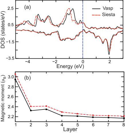
Figure 9: (color online) (a) Density of states of bulk bcc Fe, calculated with PAW (black) and NCPP (red). The NCPP gives an exchange splitting that is $\sim 0.2$ eV larger, which results in a $\sim 0.05$ $\mu_{B}$ larger magnetic moment. (b) Magnetic moments (in $\mu_{B}$/atom) of the Fe(001) surface as function of layer position (1 indicates the surface layer) calculated with PAW (black) and NCPP (red).

We optimize all structures with VASP,Kresse and Hafner (1993); Kresse and Furthmüller (1996) using the PBE functional and the parameter settings given in Sec. III. The optimized lattice constant of bulk Fe is $2.83$ Å, which is in good agreement with the experimental values of 2.87 Å.Kittel (1986) The magnetic moments per atom of bulk Fe are 2.20 $\mu_{B}$ (VASP) and 2.25 $\mu_{B}$ (SIESTA), respectively, which both are in good agreement with the experimental value of 2.22 $\mu_{B}$.Kittel (1986) The difference between the magnetic moments calculated with VASP and SIESTA can be traced to the use of norm-conserving pseudopotentials (NCPPs) in SIESTA, versus (all-electron) projector augmented waves (PAWs) in VASP. The former gives a larger exchange splitting, see Fig. 9, which gives a larger magnetic moment. VASP calculations with NCPP pseudo-potentials give a similar exchange splitting as SIESTA,de Wijs so the use of different basis sets in VASP and SIESTA, i.e., plane waves versus localized atomic orbitals, is of less importance.

The difference in calculated magnetic moments between PAWs and NCPPs persists for the Fe(001) surface. Figure 9 gives the magnetic moments as function of layer for a Fe(001) slab. The magnetic moment of a surface atom is $\sim 3$ $\mu_{B}$ and the difference between the VASP and the SIESTA results is about 3%. It is well known that $d$-band narrowing for surface atoms enhances the exchange splitting, resulting in a larger magnetic moment for the surface atoms as compared to bulk.Izquierdo et al. (2000)

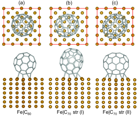
Figure 10: (color online) (a) top and side views of the most stable adsorption geometry of C₆₀ on Fe(001); Fe–C distances below 2.5 Å are indicated specifically. C₇₀ on Fe(001) in structure (I) (b) and structure (II) (c).

Table 2: Binding energies $E_{b}$ of C₆₀ and C₇₀ molecules on Fe(001) of the structures shown in Fig. 10 (total energies of unperturbed Fe(001) and isolated fullerene minus total energy of fullerene adsorbed on Fe(001)); work function $W$ of Fe(001) covered by a monolayer of fullerenes; magnetic moment $\mu$ induced on the fullerene molecules; spin polarization SP of the density of states at the Fermi level, projected on the fullerene molecules.

structure	$E_{b}$ (eV)	$W$ (eV)a	$\mu$ ($\mu_{B}$)	SP (%)
C60	2.94	4.81	0.22	0
C70(I)	2.79	4.67	0.22	0
C70(II)	2.99	4.79	0.22	40

^a Calculated work function of clean Fe(001) is 3.87 eV.

To model the adsorption of C₆₀ and C₇₀ molecules we use a slab of seven atomic layers for the Fe(001) substrate with a layer of molecules absorbed on one side of the slab, and 15 Å of vacuum thickness. The molecules and the uppermost three Fe atomic layers are allowed to relax. A dipole correction is applied to prevent spurious interactions between repeated images of the slab.Neugebauer and Scheffler (1992)

From a number of possible adsorption geometries, we have identified the structure of adsorbed C₆₀ molecules as most stable that is shown in Fig. 10(a). The edge shared by two hexagons (a 6:6 bond) is on top of a surface Fe atom, and the C₆₀ molecule is tilted such that one of the hexagons is more parallel to the surface. There are several short Fe–C bonds in the range 2.0-2.5 Å, which is an indication for chemisorption, as is confirmed by the binding energy, see Table 2. The C–C bond lengths within these two hexagons are between 1.46 and 1.52 Å, i.e., somewhat larger than the 6:6 and 5:6 bond lengths of 1.40 and 1.46 Å in an unperturbed C₆₀ molecule. Judging from the changes in bond lengths, the interaction with the Fe(001) surface seems to break the conjugation in these two hexagons somewhat. The C–C bonds in the other hexagons and pentagons are hardly perturbed by the adsorption. Upon adsorption of a monolayer of C₆₀ molecules, the work function of Fe(001) increases by 0.94 eV. The increase indicates that the C₆₀ molecule acts as an electron acceptor which is consistent with the high electron affinity of  4.5 eV of this molecule. The interaction with the ferromagnetic Fe surface induces a small magnetic moment of 0.22 $\mu_{B}$ on the C₆₀ molecule.Tran et al. (2013)

One can form a bonding geometry of the C₇₀ molecule to the Fe(001) surface that is very similar to that of C₆₀, see Fig. 10(b). This structure (I) has the edge shared by two hexagons on top of a surface Fe atom, and the C₇₀ molecule is tilted such that one of the hexagons is more parallel to the surface. C₇₀ in this structure has similar properties as C₆₀, see Table 2, but it is not the lowest energy structure. We find that in the most stable adsorption geometry, structure (II), the long axis of the C₇₀ molecule is parallel to the surface, see Fig. 10(c). Like in structure (I), in structure (II) the edge shared by two hexagons is on top of a surface Fe atom, but unlike structure (I) the two hexagons in C₇₀ have a symmetric tilt with respect to the surface. Again, there are several short Fe–C bonds in the range 2.0-2.3 Å. The C–C distances in the two hexagons involved in the adsorption are in the range 1.45-1.50 Å, again somewhat larger than the 1.39-1.47 and 1.44-1.45 Å of the 6:6 and 5:6 bonds, respectively, of the isolated C₇₀ molecule, whereas the bond lengths in the rest of the molecule are hardly changed. As structure (II) is 0.2 eV/C₇₀ molecule more stable than structure (I), we have used structure (II) in all our transport calculations.

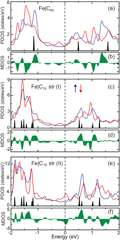
Figure 11: (color online) (a) Projected density of states PDOS $n^{\uparrow}$ of majority (blue) and $n^{\downarrow}$ of minority (red) spin states of the Fe(001)$|$C₆₀ interface, summed over all carbon atoms. Gaussian smearing with a smearing parameter of 0.05 eV is applied. The black lines give the energy levels of the isolated C₆₀ molecule. (b) Magnetization density of states MDOS $\Delta n=n^{\uparrow}-n^{\downarrow}$; (c,d) PDOS and MDOS of Fe(001)$|$C₇₀ in structure (I), and (e,f) in structure (II).

The magnetic moments induced on the C₆₀ and C₇₀ molecules are similar, and do not depend very much on the details of the structure, see Table 2. Of course only the spin polarization of the states around the Fermi level is important when studying electron transport, and not the overall polarization or magnetic moment. Figure 11(a) gives the projected density of states (PDOS) of the Fe(001)$|$C₆₀ interface, summed over all the carbon atoms. For comparison the Kohn-Sham levels of the isolated C₆₀ molecule are also given, which can be aligned with the interface DOS using the lowest $\sigma$-states of the C₆₀ molecule. The latter do not participate in the bonding to the surface, and are therefore not perturbed.

The $\pi$-states of the molecule however hybridize with states from the substrate. These molecular states can still be identified from the peaks in the PDOS, but the peaks are significantly broadened and shifted, compared to the isolated molecule. The isocahedral symmetry $I_{h}$ of the C₆₀ molecule is broken by adsorption on the Fe surface, which lifts degeneracies and splits up the peaks of the adsorbed C₆₀ molecule. In addition, the Fe(001) substrate interacts differently with the molecule for different spin states. The Fe(001) surface has prominent surface resonances in the minority spin channel for energies close to the Fermi level.Stroscio et al. (1995) The corresponding wave functions have a relatively long decay length, and one can expect these states to interact strongly with adsorbants. Indeed the minority spin states in the PDOS show a stronger perturbation with respect to the molecular $\pi$-states than the majority spin states, in particular for energies around the Fermi level.

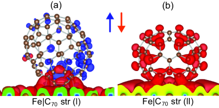
Figure 12: (color online) (a,b) Spin polarization of the LDOS at the Fe(001)$|$C₇₀ interface in structure I respectively structure II, integrated over an energy interval $[E_{F}-0.01,E_{F}+0.01]$ eV.

Comparison to the states of the isolated C₆₀ molecule allows one to label the corresponding peaks in PDOS of the adsorbed molecule. Of course adsorption broadens the peaks, and sometimes splits them. For instance, the fivefold degeneracy of the molecular HOMO is clearly lifted. In the minority spin states the LUMO, as well as the LUMO+1, which are both threefold degenerate in the isolated molecule, are split up. One of the states derived from the LUMO results in a peak in the minority spin DOS at $E_{F}-0.2$ eV, whereas other LUMO derived peaks appear above $E_{F}+0.2$ eV. It indicates that adsorption results in a net transfer of electrons to the C₆₀ molecule, which is consistent with an increase of the work function, see Table 2. At the Fermi level, $E=E_{F}$, the PDOSs of majority and minority spins are nearly equal, which implies that the spin polarization $\Delta n=n^{\uparrow}-n^{\downarrow}\approx 0$, see Fig. 11(b).

Figure 11(c) gives the PDOS of the Fe(001)$|$C₇₀ interface, with the C₇₀ in structure (I). Again for comparison the Kohn-Sham levels of the isolated C₇₀ molecule are also given. The level spectrum of C₇₀ is somewhat denser than that of C₆₀, as the molecule is slightly larger and less symmetric. Nevertheless, qualitatively the PDOS is remarkably similar to that of C₆₀. Specifically, also for C₇₀ in structure (I) one of the LUMO-derived states gives a peak in the minority spin at $E_{F}-0.2$ eV, and other LUMO-derived peaks appear above $E_{F}+0.2$ eV.

Figure 11(e) gives the PDOS of the Fe(001)$|$C₇₀ interface, with the C₇₀ in structure (II). Although qualitatively this PDOS is similar to that of C₇₀ in structure (I), there are nevertheless important differences, specifically for energies around the Fermi level. For C₇₀ in structure (II) a hybrid state with C₇₀ LUMO character gives a promiment peak in the minority spin channel that is at the Fermi level, instead of $0.2$ eV below $E_{F}$, as is the case for C₇₀ in structure (I) and for C₆₀. This means that the spin polarization at $E=E_{F}$, $\mathrm{SP}=(n^{\uparrow}-n^{\downarrow})/(n^{\uparrow}+n^{\downarrow})\approx 40$ % for C₇₀ in structure (II), which also implies that the MR in this structure is markedly different, as discussed in Sec. IV.

The difference between C₆₀ and C₇₀ in structure (I) on the one hand, and C₇₀ in structure (II) on the other, is also reflected in the wave function at the the Fermi level. Figure 12 shows the spin polarization in the local density of states (LDOS), integrated over an energy interval of $\pm 0.01$ eV around the Fermi level. The LDOS of C₇₀ in structure (II) clearly shows shows a hybrid state with clear contributions both from the C₇₀ molecule and the Fe(001) substrate, which is delocalized over the whole molecule, and has a clear minority spin character. In contrast, the LDOS of C₇₀ in structure (I) shows a hybrid state that covers only part of the molecule, and has a mixed majority/minority spin character.

References

- Fert (2008) A. Fert, Rev. Mod. Phys. 80, 1517 (2008).
- Zutic et al. (2004) I. Zutic, J. Fabian, and S. D. Sarma, Rev. Mod. Phys. 76, 323 (2004).
- Tombros et al. (2007) N. Tombros, C. Jozsa, M. Popinciuc, H. T. Jonkman, and B. J. van Wees, Nature 448, 571 (2007).
- Dediu et al. (2009) V. A. Dediu, L. E. Hueso, I. Bergenti, and C. Taliani, Nature Mater. 8, 707 (2009).
- Schmaus et al. (2011) S. Schmaus, A. Bagrets, Y. Nahas, T. K. Yamada, A. Bork, M. Bowen, E. Beaurepaire, F. Evers, and W. Wulfhekel, Nature Nanotechnol. 6, 185 (2011).
- Kawahara et al. (2012) S. L. Kawahara, J. Lagoute, V. Repain, C. Chacon, Y. Girard, S. Rousset, A. Smogunov, and C. Barreteau, Nano Lett. 12, 4558 (2012).
- miyamachi et al. (2012) T. miyamachi, M. Gruber, V. Davesne, M. Bowen, S. Boukari, L. Joly, F. Scheurer, G. Rogez, T. K. Yamada, P. Ohresser, E. Beaurepaire, and W. Wulfhekel, Nature Comm. 3, 938 (2012).
- Yoshida et al. (2013) K. Yoshida, I. Hamada, S. Sakata, A. Umeno, M. Tsukada, and K. Hirakawa, Nano Lett. 13, 481 (2013).
- Xiong et al. (2004) Z. H. Xiong, D. Wu, and V. Vardeny, Nature 427, 821 (2004).
- Santos et al. (2007) T. S. Santos, J. S. Lee, P. Migdal, I. C. Lekshmi, B. Satpati, and J. S. Moodera, Phys. Rev. Lett. 98, 016601 (2007).
- Dediu et al. (2008) V. Dediu, L. E. Hueso, I. Bergenti, A. Riminucci, F. Borgatti, P. Graziosi, C. Newby, F. Casoli, M. P. D. Jong, C. Taliani, and Y. Zhan, Phys. Rev. B 78, 115203 (2008).
- Schoonus et al. (2009) J. J. H. M. Schoonus, P. G. E. Lumens, W. Wagemans, J. T. Kohlhepp, P. A. Bobbert, H. J. M. Swagten, and B. Koopmans, Phys. Rev. Lett. 103, 146601 (2009).
- Sun et al. (2010) D. Sun, L. Yin, C. Sun, H. Guo, Z. Gai, X.-G. Zhang, T. Z. Ward, Z. Cheng, and J. Shen, Phys. Rev. Lett. 104, 236602 (2010).
- Barraud et al. (2010) C. Barraud, P. Seneor, R. Mattana, S. Fusil, K. Bouzehouane, C. Deranlot, P. Graziosi, L. Hueso, I. Bergenti, V. A. Dediu, F. Petroff, and A. Fert, Nature Phys. 6, 615 (2010).
- Schulz et al. (2011) L. Schulz, L. Nuccio, M. Willis, P. Desai, P. Shakya, T. Kreouzis, V. K. Malik, C. Bernhard, F. L. Pratt, N. A. Morley, A. Suter, G. J. Nieuwenhuys, T. Prokscha, E. Morenzoni, W. P. Gillin, and A. J. Drew, Nature Mater. 10, 39 (2011).
- Gobbi et al. (2011) M. Gobbi, F. Golmar, R. Llopis, F. Casanova, and L. E. Hueso, Adv. Mater. 23, 1609 (2011).
- Tran et al. (2012) T. L. A. Tran, T. Q. Le, J. G. M. Sanderink, W. G. van der Wiel, and M. P. de Jong, Adv. Func. Mater. 22, 1180 (2012).
- Zhang et al. (2013) X. Zhang, S. Mizukami, T. Kubota, Q. Ma, M. Oogane, H. Naganuma, Y. Ando, and T. Miyazaki, Nature Commun. 4, 1392 (2013).
- Zhang et al. (2014) X. Zhang, S. Mizukami, Q. Ma, T. Kubota, M. Oogane, H. Naganuma, Y. Ando, and T. Miyazaki, J. Appl. Phys. 115, 172608 (2014).
- Li et al. (2014) F. Li, T. Li, F. Chen, and F. Zhang, Org. Elec. 15, 1657 (2014).
- Raman et al. (2013) K. V. Raman, A. M. Kamerbeek, A. Mukherjee, N. Atodiresei, T. K. Sen, P. Lazić, V. Casiuc, D. Stalke, S. K. Mandal, and S. Blügel, Nature 493, 509 (2013).
- Sanvito (2010) S. Sanvito, Nature Phys. 6, 562 (2010).
- Cinchetti et al. (2008) M. Cinchetti, K. Heimerand, J.-P. Wüstenberg, O. Andreyev, M. Bauer, S. Lach, C. Ziegler, Y. Gao, and M. Aeschlimann, Nature Mater. 8, 115 (2008).
- Chan et al. (2010) Y.-L. Chan, Y.-J. Hung, C.-H. Wang, Y.-C. Lin, C.-Y. Chiu, Y.-L. Lai, H.-T. Chang, C.-H. Lee, Y. J. Hsu, and D. H. Wei, Phys. Rev. Lett. 104, 177204 (2010).
- Lach et al. (2012) S. Lach, A. Altenhof, K. Tarafder, F. Schmitt, M. E. Ali, M. Vogel, J. Sauther, P. M. Oppeneer, and C. Ziegler, Adv. Funct. Mater. 22, 989 (2012).
- Steil et al. (2013) S. Steil, N. Großmann, M. Laux, A. Ruffing, D. Steil, M. Wiesenmayer, S. Mathias, O. L. A. Monti, M. Cinchetti, and M. Aeschlimann, Nature Phys. 9, 242 (2013).
- Dediu (2013) V. A. Dediu, Nature Phys. 9, 210 (2013).
- Droghetti et al. (2014) A. Droghetti, S. Steil, N. Großmann, N. Haag, H. Zhang, M. Willis, W. P. Gillin, A. J. Drew, M. Aeschlimann, S. Sanvito, and M. Cinchetti, Phys. Rev. B 89, 094412 (2014).
- Shi et al. (2014) S. Shi, Z. Sun, A. Bedoya-Pinto, P. Graziosi, X. Li, X. Liu, L. Hueso, V. A. Dediu, Y. Luo, and M. Fahlman, Adv. Funct. Mater. 24, 4812 (2014).
- Giovannetti et al. (2008) G. Giovannetti, P. A. Khomyakov, G. Brocks, V. M. Karpan, J. van den Brink, and P. J. Kelly, Phys. Rev. Lett. 101, 026803 (2008).
- Rusu et al. (2010) P. C. Rusu, G. Giovannetti, C. Weijtens, R. Coehoorn, and G. Brocks, Phys. Rev. B 81, 125403 (2010).
- Bokdam et al. (2011) M. Bokdam, D. Çakır, and G. Brocks, Appl. Phys. Lett. 98, 113303 (2011).
- Atodiresei et al. (2010) N. Atodiresei, J. Brede, P. Lazić, V. Caciuc, G. Hoffmann, R. Wiesendanger, and S. Blügel, Phys. Rev. Lett. 105, 066601 (2010).
- Brede et al. (2010) J. Brede, N. Atodiresei, S. Kuck, P. Lazić, V. Caciuc, Y. Morikawa, G. Hoffmann, S. Blügel, and R. Wiesendanger, Phys. Rev. Lett. 105, 047204 (2010).
- Javaid et al. (2010) S. Javaid, M. Bowen, S. Boukari, L. Joly, J. Beaufrand, X. Chen, Y. J. Dappe, F. Schreurer, J.-P. Kappler, J. Arabski, W. Wulfhekel, M. Alouani, and E. Beaurepaire, Phys. Rev. Lett. 105, 077201 (2010).
- Tran et al. (2011) T. L. A. Tran, P. K. J. Wong, M. P. de Jong, W. G. van der Wiel, Y. Q. Zhan, and M. Fahlman, Appl. Phys. Lett. 98, 222505 (2011).
- Schwöbel et al. (2012) J. Schwöbel, Y. Fu, J. Brede, A. Dilullo, G. Hoffmann, S. Klyatskaya, M. Ruben, and R. Wiesendanger, Nature Comm. 3, 953 (2012).
- Tran et al. (2013) T. L. A. Tran, D. Çakır, P. K. J. Wong, A. B. Preobrajenski, G. Brocks, W. G. van der Wiel, and M. P. de Jong, ACS Appl. Mater. interfaces 5, 837 (2013).
- Djeghloul et al. (2013) F. Djeghloul, F. Ibrahim, M. Cantoni, M. Bowen, L. Joly, S. Boukari, P. Ohresser, F. Bertran, P. L. Fevre, P. Thakur, F. Scheurer, T. Miyamachi, R. Mattana, P. Seneor, A. Jaafar, C. Rinaldi, S. Javaid, J. Arabski, J.-P. Kappler, W. Wulfhekel, N. B. Brookes, R. Bertacco, A. Taleb-Ibrahimi, M. Alouani, E. Beaurepaire, and W. Weber, Sci. Rep. 3, 1272 (2013).
- Rocha et al. (2005) A. R. Rocha, V. M. Garcia-Suarez, S. Bailey, C. Lambert, J. Ferrer, and S. Sanvito, Nature Mater. 4, 335 (2005).
- Ning et al. (2008) Z. Ning, Y. Zhu, J. Wang, and H. Guo, Phys. Rev. Lett. 100, 056803 (2008).
- Koleini and Brandbyge (2012) M. Koleini and M. Brandbyge, Beilstein J. Nanotechnol. 3, 589 (2012).
- Liang et al. (2012) S. H. Liang, D. P. Liu, L. L. Tao, X. F. Han, and H. Guo, Phys. Rev. B 86, 224419 (2012).
- Bagrets et al. (2012) A. Bagrets, S. Schmaus, A. Jaafar, D. Kramczynski, T. K. Yamada, M. Alouani, W. Wulfhekel, and F. Evers, Nano Lett. 12, 5131 (2012).
- Karpan et al. (2007) V. M. Karpan, G. Giovannetti, P. A. Khomyakov, M. Talanana, A. A. Starikov, M. Zwierzycki, J. van den Brink, G. Brocks, and P. J. Kelly, Phys. Rev. Lett. 99, 176602 (2007).
- Karpan et al. (2008) V. M. Karpan, P. A. Khomyakov, A. A. Starikov, G. Giovannetti, M. Zwierzycki, M. Talanana, G. Brocks, J. van den Brink, and P. J. Kelly, Phys. Rev. B 78, 195419 (2008).
- Çakır et al. (2014) D. Çakır, D. M. Otálvaro, and G. Brocks, Phys. Rev. B 89, 115407 (2014).
- Datta (1995) S. Datta, Electronic Transport in Mesoscopic Systems (Cambridge University Press, Cambridge, 1995).
- Caroli et al. (1971) C. Caroli, R. Combescot, P. Nozières, and D. Saint-James, J. Phys. C: Sol. State Phys. 4, 916 (1971).
- Brandbyge et al. (2002) M. Brandbyge, J.-L. Mozos, P. Ordejón, J. Taylor, and K. Stokbro, Phys. Rev. B 65, 165401 (2002).
- Khomyakov et al. (2005) P. A. Khomyakov, G. Brocks, V. M. Karpan, M. Zwierzycki, and P. J. Kelly, Phys. Rev. B 72, 035450 (2005).
- Mahan (1990) G. D. Mahan, Many-Particle Physics, 2nd ed. (Plenum Press, New York and London, 1990).
- Jullière (1975) M. Jullière, Phys. Lett. A 54, 225 (1975).
- Blöchl (1994) P. E. Blöchl, Phys. Rev. B 50, 17953 (1994).
- Kresse and Joubert (1999) G. Kresse and D. Joubert, Phys. Rev. B 59, 1758 (1999).
- Kresse and Hafner (1993) G. Kresse and J. Hafner, Phys. Rev. B 47, 558 (1993).
- Kresse and Furthmüller (1996) G. Kresse and J. Furthmüller, Phys. Rev. B 54, 11169 (1996).
- Perdew et al. (1996) J. P. Perdew, K. Burke, and M. Ernzerhof, Phys. Rev. Lett. 77, 3865 (1996).
- Soler et al. (2002) J. M. Soler, E. Artacho, J. D. Gale, A. García, J. Junquera, P. Ordejón, and D. Sánchez-Portal, J. Phys.: Condens. Matter 14, 2745 (2002).
- Troullier and Martins (1991) N. Troullier and J. L. Martins, Phys. Rev. B 43, 1993 (1991).
- Heiney et al. (1991) P. A. Heiney, J. E. Fischer, A. R. McGhie, W. J. Romanow, A. M. Denenstein, J. P. McCauley Jr., and A. B. Smith III, Phys. Rev. Lett. 66, 2911 (1991).
- van Smaalen et al. (1994) S. van Smaalen, V. Petricek, J. L. de Boer, M. Dusek, M. A.Verheijen, and G. Meijer, Chem. Phys. Lett. 223, 323 (1994).
- (63) The transmissions of majority and minority spins are the same in the AP configuration at zero bias, .
- Mingo et al. (1996) N. Mingo, L. Jurczyszyn, F. J. Garcia-Vidal, R. Saiz-Pardo, P. L. de Andres, F. Flores, S. Y. Wu, and W. More, Phys. Rev. B 54, 2225 (1996).
- Mathon (1997) J. Mathon, Phys. Rev. B 56, 11810 (1997).
- Mathon and Umerski (1999) J. Mathon and A. Umerski, Phys. Rev. B 60, 1117 (1999).
- Kittel (1986) C. Kittel, Introduction to Solid State Physics, 7th ed. (Wiley, New York, 1986).
- (68) G. A. de Wijs, Private communication.
- Izquierdo et al. (2000) J. Izquierdo, A. Vega, L. C. Balbas, D. Sanchez-Portal, J. Junquera, E. Artacho, J. M. Soler, and P. Ordejon, Phys. Rev. B 61, 13639 (2000).
- Neugebauer and Scheffler (1992) J. Neugebauer and M. Scheffler, Phys. Rev. B 46, 16067 (1992).
- Stroscio et al. (1995) J. A. Stroscio, D. T. Pierce, A. Davies, and R. J. Celotta, Phys. Rev. Lett. 75, 2960 (1995).