Sufficient conditions to the existence for solutions of a thermoelectrochemical problem

Abstract.

A mathematical model is introduced for thermoelectrochemical phenomena in an electrolysis cell, and its qualitative analysis is focused on existence of solutions. The model consists of a system of nonlinear parabolic PDEs in conservation form expressing conservation of energy, mass and charge. On the other hand, an integral form of Newton’’s law is used to describe heat exchange at the electrolyte/electrode interface, a nonlinear radiation condition is enforced on the heat flux at the wall and a nonlinear boundary condition is considered for the electrochemical flux in order to account for Butler-Volmer kinetics. The main objective is the nonconstant character of each parameter, that is, the coefficients are assumed to be dependent on the spatial variable and the temperature. Making recourse of known estimates of solutions for some auxiliary elliptic and parabolic problems, which are explicitly determined by the Gehring-Giaquinta-Modica theory, we find sufficient smallness conditions on the data to guarantee the existence of the original solutions via the Schauder fixed point argument. These conditions may provide useful informations for numerical as well as real applications. We conclude with an example of application, namely the electrolysis of molten sodium chloride.

1. Introduction

The conservative laws are universal in the description of the physicochemical phenomena. Their particular applications depend on the transport coefficients behavior. The introduction of the thermal effects into physicochemical devices are being addressed by applied mathematicians [27]. Quantitative description of the heat rate data is discussed in [4, 16]. The model parameters (such as the electrical mobilities $u_{i}$, and the thermal conductivity $k$, among others) are assumed to be constant positive quantities whose values are specified to numerical simulations. Our first shortcoming is that these coefficients are commonly discontinuous.

In view of the above discussion, we develop a thermoelectrochemical model for an electrolyte domain. Our second shortcoming is that the physicochemical phenomena truly pass on the boundary of the domain. We mention to [33] a mathematical modeling of the interaction of electric, thermal, and diffusion processes in infinitely diluted solutions of electrolytes. The production of nuclear grade heavy water, including water electrolysis, distillation, and chemical exchange processes, provide a process matched to the feed supply [23, 31]. We refer to [21] a mathematical model of Li-ion batteries based exclusively on universally accepted principles of nonequilibrium thermodynamics and the assumption of the one step intercalation reaction at the interface of electrolyte and active particles; and to [24, 32] other attractive thermoelectrochemical approaches.

In thermoelectrochemical modeling, the force-flux relations are (see, at the steady-state, [8] and the references therein)

$${\bf q}= -\mathsf{K}\nabla\theta-R\theta^{2}\sum_{i=1}^{I}D^{\prime}_{i}\nabla c_{i}-\Pi\sigma\nabla\phi;$$ (1)

$${\bf J}_{i}= -c_{i}S_{i}\nabla\theta-D_{i}\nabla c_{i}-u_{i}c_{i}\nabla\phi;\quad(i=1,\cdots,I)$$

$${\bf j}= -\alpha\sigma\nabla\theta-F\sum_{i=1}^{I}z_{i}D_{i}\nabla c_{i}-\sigma\nabla\phi.$$

Here, ${\bf q}$, ${\bf J}_{i}$ and $\bf j$ are, respectively, the measurable heat flux (in W$\cdot$m^-2), the ionic flux of component $i$ (in mol$\cdot$m${}^{-2}\cdot$s^-1), and the electric current density (in C$\cdot$m${}^{-2}\cdot$s^-1). The unknown functions are the temperature $\theta$, the molar concentration vector ${\bf c}=(c_{1},\cdots,c_{I})$, and the electric potential $\phi$. Hereafter the subscript $i$ stands for the correspondence to the ionic component $i$ intervener in the reaction process. As the problem involves several symbols, we summarize their notation in Appendix. In particular, $\mathsf{K}$ denotes the thermal conductivity tensor, reflecting anisotropic properties of the medium. Also the Peltier coefficient $\Pi$ can be a tensor [3]. By this reason, we keep both $\alpha$ and $\Pi$ as known functions, although the first Kelvin relation correlates $\Pi$ with the Seebeck coefficient $\alpha$. All transport coefficients can be either experimentally measured or calculated as dependent on temperature and spatial variable, while the Soret effect and the related Dufour effect include the concentration of the correspondent ionic component [17, 22].

Dealing with these issues, our main concerns are: in the physical point of view to introduce thermal radiation on one part of the boundary, to approach the Butler-Volmer equation on other part of the boundary; and in the mathematical point of view to find sufficient explicit conditions on the data to the existence of solutions, under minimal assumptions on the transport coefficients, as consequence of the fixed point theory. The key of an integrability exponent larger than $n$ for the solution (say in $n$ space dimensions) is the need of making severe restrictions on the corresponding leading coefficient function - as is carried out in the literature [10].

2. Statement of the problem and main theorem

Let $T>0$ be an arbitrary (but preassigned) time, and $\Omega$ represent an electrolysis cell, which consists (as in general) of two electrodes and an electrolyte. We abbreviate $Q_{T}=\Omega\times]0,T[$.

From the conservation of energy, the mass balance equations, and the conservation of electric charge, we derive, respectively, in $Q_{T}$

$$\rho c_{\mathrm{p}}\frac{\partial\theta}{\partial t}+\nabla\cdot{\bf q}=0;$$ (2)

$$\frac{\partial c_{i}}{\partial t}+\nabla\cdot{\bf J}_{i}=0;$$ (3)

$$\nabla\cdot{\bf j}=0,$$ (4)

where the density $\rho$ and the specific heat capacity $c_{\mathrm{p}}$ (at constant volume) are assumed to be (positive) constants. The absence of external forces, assumed in (2)-(4), is due to their occurrence at the surface of the electrodes.

The boundary $\partial\Omega$ is decomposed into four pairwise disjoint open subsets $\Gamma_{l}$, $l=$ a, c, w, o, representing the anode, the cathode, the wall, and the (remaining) outer, respectively, surfaces such that (cf. Fig. 1)

$$\partial\Omega=\overline{\Gamma}_{\rm a}\cup\overline{\Gamma}_{\rm c}\cup\overline{\Gamma}_{\rm w}\cup\overline{\Gamma}_{\rm o}.$$

For the sake of simplicity, we call the electrode/electrolyte interface $\Gamma_{\rm e}=\Gamma_{\rm a}\cup\Gamma_{\rm c}$ by simply $\Gamma$, and we set $\Sigma_{T}=\Gamma_{\mathrm{w}}\times]0,T[$. Hence further, for each $l=$ a, c, w, $\theta_{l}$ represents a given temperature at $\Gamma_{l}$, and $\bf n$ is the outward unit normal to the boundary $\partial\Omega$.

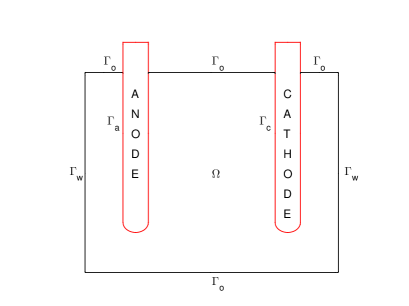
Figure 1. Schematic saggital representation of an electrolytic cell (with corners being smoothed by circumferences)

The parabolic-elliptic system (2)-(4) is accomplished by the following boundary conditions. For a.e. in $]0,T[$, we consider the heat balance described by the global Newton law of cooling

$$\int_{\Gamma_{\mathrm{a}}}{\bf q}\cdot{\bf n}\mathrm{ds}+\int_{\Gamma_{\mathrm{c}}}{\bf q}\cdot{\bf n}\mathrm{ds}=\int_{\Gamma_{\mathrm{e}}}h_{\mathrm{C}}(\theta-\theta_{\mathrm{e}})\mathrm{ds},\qquad\theta_{\mathrm{e}}=\left\{\begin{array}[]{ll}\theta_{\mathrm{a}}&\mbox{on }\Gamma_{\mathrm{a}}\\ \theta_{\mathrm{c}}&\mbox{on }\Gamma_{\mathrm{c}}\end{array}\right.,$$ (5)

where $h_{\rm C}$ denotes the conductive heat transfer coefficient. By the constitutive law (1) of $\bf q$, the left-hand side of (5) says that the heat generated is divided into the irreversible reaction heat due to efficiency losses of the electrode reaction, and the reversible reaction heat mainly due to the entropy change of the electrode reaction which is called Peltier heat and changes sign with changing current direction (cf. [15]).

A gas bubble behavior at a hydrogen-evolution electrode was reported by some researchers [5, 19, 30]. This hydrogen gas generated at the cathode causes turbulence of water or wastewater flow [6]. At each electrode/electrolyte interface ($l=$ a, c), we consider

$$-Fz_{i}{\bf J}_{i}\cdot{\bf n}_{l}=g_{i,l}(\cdot,\theta,\phi).$$

Here, $g_{i,l}$ may represent the generalized Butler-Volmer kinetics that is composed by the involved charge and mass balances in the charge-transfer reaction under illumination [28], and the Butler-Volmer expression itself

$$J_{l}\left(\exp\left[\frac{\beta_{i}s_{l}F\eta}{R\theta}\right]-\exp\left[-\frac{(1-\beta_{i})s_{l}F\eta}{R\theta}\right]\right),$$ (6)

where $J_{l}$ represents the transfer (exchange) current density due to the electrode reaction, $s_{l}$ is the stoichiometric coefficient of electrons in the anode/cathode ($l=$ a, c), $\beta_{i}$ is the transfer coefficient ($i=1,\cdots,I$), and $\eta=\phi-\phi_{\rm eq}$ denotes the surface overpotential.

Although the electroneutrality assumption says that ${\bf j}=\sum_{i=1}^{I}z_{i}F{\bf J}_{i}$, we consider on $\Gamma\times]0,T[$

$$-{\bf j}\cdot{\bf n}=g,$$ (7)

with $g$ being a prescribed surface electric current assumed to be tangent to the surface for all $t>0$. We refer as an open problem the nonlocal Dirichlet boundary condition for the electric potential, $\phi=j(I)$ [12], on the part of the boundary ($\Gamma_{\mathrm{e}}$) where the device is connected to the circuit, with $j$ being a nonlinear function and $I=\int_{\Gamma_{\mathrm{e}}}\sigma(\theta)\frac{\partial\phi}{\partial n}$ denoting the total current, when the voltage drop across the electrical circuits is not prescribed but is coupled to the remainder circuit.

Let temperature fulfill the radiative condition over $\Gamma_{\mathrm{w}}\times]0,T[$

$${\bf q}\cdot{\bf n}=h_{\mathrm{R}}|\theta|^{\ell-2}\theta-\gamma.$$ (8)

This general exponent $\ell\geq 2$ [7] accounts for the radiation behavior of the heavy water electrolysis [11, 20], namely the Stefan-Boltzmann radiation law if $\ell=5$ with $h_{\rm R}$ denoting the radiative heat transfer coefficient, i.e. $h_{\mathrm{R}}=\sigma_{\rm SB}\epsilon$, and $\gamma=\sigma_{\rm SB}\alpha\theta_{\mathrm{w}}^{4}$. The parameters, the emissivity $\epsilon$ and the absorptivity $\alpha$, both depend on the spatial variable and the temperature function $\theta$.

The following no outflows are considered:

$$\mathrm{on}\ \Gamma_{\rm o}\times]0,T[, \qquad\mathbf{q}\cdot{\bf n}=0;$$ (9)

$$\mathrm{on}\ \left(\Gamma_{\rm w}\cup\Gamma_{\rm o}\right)\times]0,T[, \qquad{\bf J}_{i}\cdot{\bf n}={\bf j}\cdot{\bf n}=0,\qquad(i=1,\cdots,I).$$ (10)

Finally, the following initial conditions for all $x$ in $\Omega$ are assumed:

$$\theta(x,0)=\theta_{0}(x),\quad c_{i}(x,0)=c_{i}^{0}(x),\quad i=1,\cdots,I.$$ (11)

In the framework of Sobolev and Lebesgue functional spaces, we use the following spaces of test functions:

$$V_{p,\ell}(Q_{T})= \{v\in L^{p}(0,T;W^{1,p}(\Omega)):\ v|_{\Sigma_{T}}\in L^{\ell}(\Sigma_{T})\};$$

$$V_{p}(\Omega)= \{v\in W^{1,p}(\Omega):\ \int_{\partial\Omega}v\mathrm{ds}=0\},$$

with their usual norms, $p,\ell>1$.

In order to derive our variational problem, we note that every ionic mobility $u_{i}=z_{i}D_{i}F/(R\theta)$ satisfies the Nernst-Einstein relation $\sigma_{i}=F{z_{i}}{}u_{i}c_{i}$, with $\sigma_{i}=t_{i}\sigma$ representing ionic conductivity, and $t_{i}$ is the transference number (or transport number) of species $i$.

Then our variational problem under study is:

($\mathcal{P}$) Find the triple temperature–concentration–potential $(\theta,{\bf c},\phi)$ such that verifies the variational problem:

$$\rho c_{\mathrm{p}}\int_{0}^{T}\langle\partial_{t}\theta,v\rangle\mathrm{dt}+\int_{Q_{T}}(\mathsf{K}(\cdot,\theta)\nabla\theta)\cdot\nabla v\mathrm{dx}\mathrm{dt}+\int_{\Sigma_{T}}h_{\mathrm{R}}(\cdot,\theta)|\theta|^{\ell-2}\theta v\mathrm{ds}\mathrm{dt}+$$

$$+\int_{0}^{T}\int_{\Gamma}h_{\mathrm{C}}(\cdot,\theta)\theta v\mathrm{ds}\mathrm{dt}=\int_{0}^{T}\int_{\Gamma}h_{\mathrm{C}}(\cdot,\theta)\theta_{\mathrm{e}}v\mathrm{ds}\mathrm{dt}+\int_{\Sigma_{T}}\gamma(\cdot,\theta)v\mathrm{ds}\mathrm{dt}$$

$$-\int_{Q_{T}}\left(R\theta^{2}\sum_{i=1}^{I}D_{i}^{\prime}(\cdot,c_{i},\theta)\nabla c_{i}+\Pi(\cdot,\theta)\sigma(\cdot,\theta)\nabla\phi\right)\cdot\nabla v\mathrm{dx}\mathrm{dt},$$

$$\forall v\in V_{p^{\prime},\ell}(Q_{T});$$ (12)

$$\int_{0}^{T}\langle\partial_{t}c_{i},v\rangle\mathrm{dt}+\int_{Q_{T}}D_{i}(\cdot,\theta)\nabla c_{i}\cdot\nabla v\mathrm{dx}\mathrm{dt}=\int_{0}^{T}\int_{\Gamma}g_{i}(\cdot,\theta,\phi)v\mathrm{ds}\mathrm{dt}$$

$$-\int_{Q_{T}}\left(c_{i}S_{i}(\cdot,c_{i},\theta)\nabla\theta+\frac{t_{i}}{Fz_{i}}\sigma(\cdot,\theta)\nabla\phi\right)\cdot\nabla v\mathrm{dx}\mathrm{dt},$$

$$\forall v\in L^{p^{\prime}}(0,T;W^{1,p^{\prime}}(\Omega)),\quad i=1,\cdots,I;$$ (13)

$$\int_{\Omega}\sigma(\cdot,\theta)\nabla\phi\cdot\nabla v\mathrm{dx}=\int_{\Gamma}gv\mathrm{ds}$$

$$-\int_{\Omega}\left(\alpha(\cdot,\theta)\sigma(\cdot,\theta)\nabla\theta+F\sum_{i=1}^{I}z_{i}D_{i}(\cdot,\theta)\nabla c_{i}\right)\cdot\nabla v\mathrm{dx},$$

$$\forall v\in V_{p^{\prime}}(\Omega),\qquad\mbox{a.e. in }[0,T[,$$ (14)

where $p^{\prime}$ accounts for the conjugate exponent of $p$: $p^{\prime}=p/(p-1)$.

We assume

(H1):

The electrical conductivity, Peltier, Seebeck, Soret, Dufour, and diffusion coefficients $\sigma,\Pi,\alpha,S_{i},D_{i}^{\prime},D_{i}$ ($i=1,\cdots,I$) are Carathéodory functions, i.e. measurable with respect to $x\in\Omega$ and continuous with respect to other variables, such that

$$\exists\sigma_{\#},\sigma^{\#}>0:\qquad \sigma_{\#}\leq\sigma(x,e)\leq\sigma^{\#};$$ (15)

$$\exists\Pi^{\#}>0:\qquad |\Pi(x,e){\bf a}|\leq\Pi^{\#}|{\bf a}|;$$ (16)

$$\exists\alpha^{\#}>0:\qquad |\alpha(x,e)|\leq\alpha^{\#};$$ (17)

$$\exists S_{i}^{\#}>0:\qquad |dS_{i}(x,d,e)|\leq S_{i}^{\#};$$ (18)

$$\exists(D_{i}^{\prime})^{\#}>0:\qquad Re^{2}|D_{i}^{\prime}(x,d,e)|\leq(D_{i}^{\prime})^{\#};$$ (19)

$$\exists D_{i}^{\#}>0:\qquad F|z_{i}|D_{i}(x,e)\leq D_{i}^{\#};$$ (20)

$$\exists(D_{i})_{\#}>0:\qquad D_{i}(x,e)\geq(D_{i})_{\#},$$ (21)

a.e. $x\in\Omega$, for all ${\bf a}\in\mathbb{R}^{n}$, and for all $d,e\in\mathbb{R}$.

(H2):

The thermal conductivity $\mathsf{K}:\Omega\times\mathbb{R}\rightarrow\mathbb{M}_{n\times n}$ is a Carathéodory tensor, where $\mathbb{M}_{n\times n}$ denotes the set of $n\times n$ matrices, such that

$$\exists k_{\#}>0:\quad K_{jl}(x,e)\xi_{j}\xi_{l}\geq k_{\#}|\xi|^{2},\quad\mbox{a.e. }x\in\Omega,\quad\forall e\in\mathbb{R},$$ (22)

for all $\xi\in\mathbb{R}^{n}$, under the summation convention over repeated indices: $\mathsf{A}{\bf a}\cdot{\bf b}=A_{jl}a_{j}b_{l}={\bf b}^{\top}\mathsf{A}{\bf a}$; and

$$\exists k^{\#}>0:\quad|K_{jl}(x,e)|\leq k^{\#},\quad\mbox{a.e. }x\in\Omega,\quad\forall e\in\mathbb{R},$$ (23)

for all $j,l\in\{1,\cdots,n\}$.

(H3):

The boundary operator $h_{\mathrm{R}}$ is a Carathéodory function from $\Gamma_{\mathrm{w}}\times\mathbb{R}$ into $\mathbb{R}$ such that

$$\exists b_{\#},b^{\#}>0:\quad b_{\#}\leq h_{\mathrm{R}}(x,e)\leq b^{\#}\quad\mbox{a.e. }x\in\Gamma_{\mathrm{w}},\quad\forall e\in\mathbb{R}.$$ (24)

(H4):

The transference coefficient $t_{i}\in L^{\infty}(\Omega)$ is such that

$$\exists t_{i}^{\#}>0:\quad 0\leq t_{i}(x)\leq F|z_{i}|t_{i}^{\#},\quad\mbox{a.e. }x\in\Omega.$$ (25)

(H5):

For some $\delta>0$, $g\in L^{2+\delta}(\Gamma)$ such that $\int_{\Gamma}g\mathrm{ds}=0$.

(H6):

For some $\delta>0$, $\theta_{\mathrm{e}}\in L^{2+\delta}(\Gamma\times]0,T[)$, and the boundary operators $\gamma$ and $h_{\mathrm{C}}$ are Carathéodory functions from $\Gamma_{\mathrm{w}}\times]0,T[\times\mathbb{R}$ and $\Gamma\times]0,T[\times\mathbb{R}$, respectively, into $\mathbb{R}$, i.e. measurable with respect to $(x,t)$ and continuous with respect to the real variable. Moreover, they satisfy

$$\exists\gamma_{\mathrm{w}}\in L^{2+\delta}(\Sigma_{T}): \qquad|\gamma(x,t,e)|\leq\gamma_{\mathrm{w}}(x,t),\quad\mbox{a.e. }x\in\Gamma_{\mathrm{w}};$$ (26)

$$\exists h_{\mathrm{C}}^{\#}>0: \qquad 0\leq h_{\mathrm{C}}(x,t,e)\leq h_{\mathrm{C}}^{\#},\quad\mbox{a.e. }x\in\Gamma,$$ (27)

a.e. $t\in]0,T[$, and for all $e\in\mathbb{R}$.

(H7):

For some $\delta>0$, and for each $i=1,\cdots,I$, the boundary operator $g_{i}=g_{i,\mathrm{a}}\chi_{\Gamma_{\mathrm{a}}}+g_{i,\mathrm{c}}\chi_{\Gamma_{\mathrm{c}}}$ is a Carathéodory function from $\Gamma\times]0,T[\times\mathbb{R}\times\mathbb{R}$ into $\mathbb{R}$ and there exists $\gamma_{i}\in L^{2+\delta}(\Gamma\times]0,T[)$ such that

$$\exists g_{i}^{\#}\geq 0:\quad|g_{i}(x,t,e,d)|\leq\gamma_{i}(x,t)+g_{i}^{\#}(|d|+|e|),$$ (28)

a.e. $(x,t)\in\Gamma\times]0,T[$, and for all $e,d\in\mathbb{R}$.

(H8):

For some $\delta>0$, $\theta_{0},c_{i}^{0}\in L^{2+\delta}(\Omega)$, $i=1,\cdots,I$.

For the sake of simplicity, we assume in (H5)-(H8) the same designation $\delta>0$. Note that (28) is verified for a truncated version of the Butler-Volmer expression (6).

The main interest of the mathematical model under study (governing equations and boundary conditions) is strictly related to real world applications (thermoelectrochemical phenomena in an electrolysis cell $\Omega$). In this respect, the consideration of a number $n$ of space dimensions greater than $3$ is not really relevant. From the mathematical point of view, the broader dimensional range, if available, is more meaningful in fact. Therefore, we state our main result in the unified way.

Theorem 2.1.

Under the hypothesis (H1)-(H8), there exists a solution

$$(\theta,{\bf c},\phi)\in V_{p,\ell}(Q_{T})\times[L^{p}(0,T;W^{1,p}(\Omega))]^{I}\times V_{p}(\Omega),$$

for some $p>2$, to (12)-(14) with the initial condition (11) if provided by the smallness conditions (58), and (59)-(60).

Remark 2.1.

The existence of $p$ is restricted to $[2,2+\delta]$, where $\delta>0$ is chosen smaller than min$\{2/[n(\upsilon-1)],1/(\varkappa-1)\}$ with $\upsilon,\varkappa>1$ being well-determined constants by the Gehring-Giaquinta-Modica theory [1, 2, 14].

3. Strategy of the proof of Theorem 2.1

In this section we discuss the key of the proof, and we recall a known result for the solvability. The proof of Theorem 2.1 is based on the Schauder fixed point theorem [35]. We freeze the concentrations-temperature pair $({\bf c},\theta)$ in the closed convex set

$$\mathcal{K}=\{({\bf v},v)\in[L^{p}(0,T;W^{1,p}(\Omega))]^{I}\times V_{p,\ell}(Q_{T}):\ \|\nabla v\|_{p,Q_{T}}+\|v\|_{\ell,\Sigma_{T}}\leq R,$$

$$\|\nabla v_{i}\|_{p,Q_{T}}+\|v_{i}\|_{p,Q_{T}}\leq R_{i},\ i=1,\cdots,I\},$$

where $p,\ell\geq 2$, and we built the well defined functional $\mathcal{T}$ such that

$$({\bf c},\theta)\in\mathcal{K}\mapsto\phi\in V_{p}(\Omega)\mapsto({\bf\Psi},\Theta),$$ (29)

where $\phi$, $\bf\Psi$, and $\Theta$ are the unique functions given at Propositions 4.1, 4.2, and 4.3, respectively. Their proofs rely on existence results due to a weak reverse Hölder inequality for local solutions [1, 2, 14]. For reader’s convenience, we recall the parabolic existence result [2, 14].

Theorem 3.1.

Let $\Omega$ be a $C^{1}$ domain, $T>0$, and the assumptions (22)-(24) be fulfilled. There exists $\upsilon>1$ such that for any $0<\delta<2/[n(\upsilon-1)]$ and $p\in[2,2+\delta]$ if ${\bf f}\in{\bf L}^{2+\delta}(Q_{T})$, $f\in L^{2+\delta}(\Gamma\times]0,T[)$, $H\in L^{2+\delta}(\Sigma_{T})$ and $u_{0}\in L^{2+\delta}(\Omega)$, then the variational problem

$$\int_{0}^{T}\langle\partial_{t}u,v\rangle\mathrm{dt}+\int_{Q_{T}}(\mathsf{K}\nabla u)\cdot\nabla v\mathrm{dx}\mathrm{dt}+\int_{\Sigma_{T}}h_{\mathrm{R}}(u)|u|^{\ell-2}uv\mathrm{ds}\mathrm{dt}=$$

$$=\int_{Q_{T}}{\bf f}\cdot\nabla v\mathrm{dx}\mathrm{dt}+\int_{0}^{T}\int_{\Gamma}fv\mathrm{ds}\mathrm{dt}+\int_{\Sigma_{T}}Hv\mathrm{ds}\mathrm{dt},\quad\forall v\in V_{p^{\prime},\ell}(Q_{T}),$$ (30)

has a solution $u$ in $L^{p,\infty}(Q_{T})\cap V_{p,\ell+p-2}(Q_{T})$ such that $\partial_{t}u\in[V_{p^{\prime},\ell}(Q_{T})]^{\prime}$, and it verifies

$${\rm ess}\sup_{t\in[0,T]}\|u\|_{p,\Omega}^{p}(t)\leq\mathcal{H}(k_{\#},b_{\#},p)\exp\left[(p-1)T\right];$$ (31)

$$\|u\|^{\ell+p-2}_{\ell+p-2,\Sigma_{T}}\leq(b_{\#})^{-1}\mathcal{H}(k_{\#},b_{\#},p)\left(1+(p-1)T\exp\left[(p-1)T\right]\right);$$ (32)

$$\|\nabla u\|_{p,Q_{T}}\leq\mathcal{C}(k_{\#})^{-1}\left[\sqrt{k_{\#}\mathcal{H}(k_{\#},b_{\#},2)\left(1+T\exp\left[T\right]\right)}+\right.$$

$$+\left.\sqrt{1+k_{\#}}\left(\|{\bf f}\|_{p,Q_{T}}+K_{2n/(n+1)}\left[\|f\|_{p,\Gamma\times]0,T[}+\|H\|_{p,\Sigma_{T}}\right]\right)\right],$$ (33)

with

$$\mathcal{H}(k_{\#},b_{\#},p)=\|u_{0}\|_{p,\Omega}^{p}+\left({p-1\over k_{\#}}\right)^{p/2}\|{\bf f}\|_{p,Q_{T}}^{p}+$$

$$+\frac{p(\ell-1)}{(\ell+p-2)b_{\#}^{(p-1)/(\ell-1)}}\int_{\Sigma_{T}}|H|^{\frac{\ell+p-2}{\ell-1}}\mathrm{ds}\mathrm{dt}+$$

$$+(p-1)\left(\left(\frac{p^{2}}{2k_{\#}(p-1)}\right)^{1/(p-1)}+1\right)K_{2n/(n+1)}^{2/(p-1)}|\Omega|^{[(p-1)n]^{-1}}\|f\|_{p^{\prime},\Gamma\times]0,T[}^{p^{\prime}}.$$

Here, $K_{2n/(n+1)}$ stands for the continuity constant of the trace embedding $W^{1,2n/(n+1)}(\Omega)\hookrightarrow L^{2}(\Gamma)$, and $\mathcal{C}$ is a positive constant depending only on $\upsilon$, $p$, $n$, and $\Omega$. In particular, if $b_{\#}=0$ and $f=0$, then (31) and (33) remain true by replacing $\mathcal{H}(k_{\#},b_{\#},p)$ by

$$\mathcal{H}(k_{\#},p)=\|u_{0}\|_{p,\Omega}^{p}+\left({p-1\over k_{\#}}\right)^{p/2}\|{\bf f}\|_{p,Q_{T}}^{p}+$$

$$+(p-1)\left(\left(\frac{p^{2}}{2k_{\#}(p-1)}\right)^{\frac{1}{p-1}}+1\right)K_{2n/(n+1)}^{2/(p-1)}|\Omega|^{[(p-1)n]^{-1}}\|H\|_{p^{\prime},\Sigma_{T}}^{p^{\prime}}.$$ (34)

Remark 3.1.

By the Aubin-Lions theorem [25], we have that $u\in L^{p}(Q_{T})$, and the initial condition $u(0)=u_{0}$ makes sense at least in $L^{p}(\Omega)$.

4. Existence of auxiliary solutions

Let us establish the existence of solutions according to Section 3. Fix $\delta\in]0,2/[n(\upsilon-1)][$ with $\upsilon>1$ being given from Theorem 3.1.

First, let us recall the existence of the required auxiliary potential solving a second order elliptic equation of divergence form with a discontinuous leading coefficient.

Proposition 4.1 (Auxiliary potential).

Let $\delta>0$, $t\in]0,T[$, $\theta(t),c_{i}(t)\in W^{1,2+\delta}(\Omega)$, for every $i=1,\cdots,I$, $g\in L^{2+\delta}(\partial\Omega)$ verify $\int_{\partial\Omega}g\mathrm{ds}=0$, and (15), (17), and (20) hold. There exists $\varkappa>1$ such that the Neumann problem (14) is uniquely (up to constants) solvable in $W^{1,p}(\Omega)$ for any $p\in[2,2+\delta]\cap[2,2+1/(\varkappa-1)[$. Moreover, for each $]0,T[$ we have

$$\sigma_{\#}\|\nabla\phi\|_{2,\Omega}\leq K\|g\|_{2,\Gamma}+\sigma^{\#}\alpha^{\#}\|\nabla\theta\|_{2,\Omega}+\sum_{j=1}^{I}D_{j}^{\#}\|\nabla c_{j}\|_{2,\Omega};\$$ (35)

$$\|\nabla\phi\|_{p,\Omega}\leq M_{1}\|\nabla\phi\|_{2,\Omega}+M_{2}(\sigma_{\#})^{-1}\sqrt{1+\sigma_{\#}}\|{\mathcal{F}}(\theta,{\bf c})\|_{p,\Omega}+$$

$$+M_{3}(\sigma_{\#})^{-1}\sqrt{2+{2^{-1/n}\sigma_{\#}}}\|g\|_{p,\Gamma},\quad$$ (36)

where $K$ stands for a positive constant depending on $n$ and $\Omega$,

$${\mathcal{F}}(\theta,{\bf c})=\sigma^{\#}\alpha^{\#}|\nabla\theta|+\sum_{j=1}^{I}D_{j}^{\#}|\nabla c_{j}|,$$

and $M_{1}$, $M_{2}$ and $M_{3}$ are positive constants depending on $n$, $p$, $\varkappa$, and $\Omega$.

Proof.

The existence of the weak unique solution satisfying (35) is classical (for details see, for instance, [9]). A similar proof of the regularity estimate (36) can be found in [1, 2]. ∎

The existence of the auxiliary concentrations-temperature pair $({\bf\Psi},\Theta)$ is consequence of Theorem 3.1 as follows.

Proposition 4.2 (Auxiliary concentrations).

Let $\theta\in L^{p}(0,T;W^{1,p}(\Omega))$, and $\phi\in V_{p}(\Omega)$ be in accordance with Proposition 4.1, with $p\in[2,2+\delta]\cap[2,2+1/(\varkappa-1)[$. Under the assumptions (15), (18), (20)-(21), (25), and (28), there exists a function ${\bf\Psi}\in[L^{p}(0,T;W^{1,p}(\Omega))]^{I}$ being the unique solution to the variational problem, for each $i=1,\cdots,I$,

$$\int_{0}^{T}\langle\partial_{t}\Psi_{i},v\rangle\mathrm{dt}+\int_{Q_{T}}D_{i}(\theta)\nabla\Psi_{i}\cdot\nabla v\mathrm{dx}\mathrm{dt}=\int_{0}^{T}\int_{\Gamma}g_{i}(\theta,\phi)v\mathrm{ds}\mathrm{dt}$$

$$-\int_{Q_{T}}\left(c_{i}S_{i}(c_{i},\theta)\nabla\theta+\frac{t_{i}}{Fz_{i}}\sigma(\theta)\nabla\phi\right)\cdot\nabla v\mathrm{dx}\mathrm{dt},$$ (37)

for all $v\in L^{p^{\prime}}(0,T;W^{1,p^{\prime}}(\Omega))$. In particular, $\partial_{t}{\bf\Psi}\in[L^{p}(0,T;[W^{1,p^{\prime}}(\Omega)]^{\prime})]^{I}$, and ${\bf\Psi}\in[C([0,T];L^{2}(\Omega))]^{I}$. Moreover, for every $i=1,\cdots,I$, we have

$$\|\Psi_{i}\|_{p,Q_{T}}^{p}\leq T\|\Psi_{i}\|_{\infty,p,Q_{T}}^{p}\leq T\exp\left[(p-1)T\right]\left[\|c_{0,i}\|_{p,\Omega}^{p}+\right.$$

$$+\left({p-1\over(D_{i})_{\#}}\right)^{p/2}\left(S_{i}^{\#}\|\nabla\theta\|_{p,Q_{T}}+t_{i}^{\#}\sigma^{\#}\|\nabla\phi\|_{p,Q_{T}}\right)^{p}+$$

$$+\left(\left(\frac{p^{2}(p-1)^{p-2}}{2(D_{i})_{\#}}\right)^{\frac{1}{p-1}}+p-1\right)K_{2n/(n+1)}^{2p^{\prime}/p}|\Omega|^{p^{\prime}(pn)^{-1}}\left(\|\gamma_{i}\|_{p^{\prime},\Gamma\times]0,T[}+\right.$$

$$\left.\left.+g_{i}^{\#}K_{pn/(n+p-1)}|\Omega|^{1-1/p}\left(\|\nabla\theta\|_{p,Q_{T}}+\|\theta\|_{p,Q_{T}}+P_{p}\|\nabla\phi\|_{p,Q_{T}}\right)\right)^{p^{\prime}}\right];\quad$$ (38)

$$\|\nabla\Psi_{i}\|_{p,Q_{T}}\leq\mathcal{C}(D_{i})_{\#}^{-1}\left[\sqrt{(D_{i})_{\#}(1+T\exp[T])}\|c_{0,i}\|_{2,\Omega}+\mathcal{G}_{i}^{\#}+\right.$$

$$+X_{i}\|\nabla\phi\|_{2,Q_{T}}+Y_{i}\|\nabla\phi\|_{p,Q_{T}}+$$

$$\left.+\left(S_{i}^{\#}\mathcal{Z}(|Q_{T}|^{1/2-1/p},(D_{i})_{\#},1)+\mathcal{Q}_{i}\right)(\|\nabla\theta\|_{p,Q_{T}}+\|\theta\|_{p,Q_{T}})\right],\quad$$ (39)

with

$$\mathcal{G}_{i}^{\#}=K_{2n/(n+1)}\left(\sqrt{(1+T\exp[T])(2+(D_{i})_{\#})|\Omega|^{1/n}}\|\gamma_{i}\|_{2,\Gamma\times]0,T[}+\right.$$

$$\left.+\sqrt{1+(D_{i})_{\#}}\|\gamma_{i}\|_{p,\Gamma\times]0,T[}\right);$$ (40)

$$X_{i}=\sqrt{1+T\exp[T]}\left(t_{i}^{\#}\sigma^{\#}+g_{i}^{\#}\sqrt{2+(D_{i})_{\#}}|\Omega|^{\frac{1+1/n}{2}}K_{2n/(n+1)}^{2}P_{2}\right);$$ (41)

$$Y_{i}=\sqrt{1+(D_{i})_{\#}}\left(t_{i}^{\#}\sigma^{\#}+g_{i}^{\#}K_{2n/(n+1)}K_{pn/(n+p-1)}|\Omega|^{1-1/p}P_{p}\right);$$ (42)

$$\mathcal{Q}_{i}=K_{2n/(n+1)}g_{i}^{\#}\left(\sqrt{1+(D_{i})_{\#}}K_{pn/(n+p-1)}|\Omega|^{1-1/p}+\right.$$

$$\left.+\sqrt{(1+T\exp[T])(2+(D_{i})_{\#})|\Omega|^{1/n}}K_{2n/(n+1)}|\Omega|^{1-1/p}T^{1/2-1/p}\right);$$ (43)

$$\mathcal{Z}(a,d,e)=a\sqrt{1+T\exp[T]}+e\sqrt{1+d},\quad a,d,e>0,$$ (44)

and $P_{p}$ stands for the Poincaré constant correspondent to the space exponent $p$.

Proof.

The existence of the required auxiliary concentrations is consequence of Theorem 3.1 and Remark 3.1. In particular, we have

$$\|\nabla\Psi_{i}\|_{p,Q_{T}}\leq\mathcal{C}(D_{i})_{\#}^{-1}\left[\sqrt{(D_{i})_{\#}(1+T\exp[T])}\|c_{0,i}\|_{2,\Omega}+H_{i}(\theta,\phi)+\right.$$

$$+t_{i}^{\#}\sigma^{\#}\left(\sqrt{1+T\exp[T]}\|\nabla\phi\|_{2,Q_{T}}+\sqrt{1+(D_{i})_{\#}}\|\nabla\phi\|_{p,Q_{T}}\right)$$

$$\left.+S_{i}^{\#}\left(\sqrt{1+T\exp[T]}\|\nabla\theta\|_{2,Q_{T}}+\sqrt{1+(D_{i})_{\#}}\|\nabla\theta\|_{p,Q_{T}}\right)\right],$$

with

$$H_{i}(\theta,\phi)=\mathcal{G}_{i}^{\#}+$$

$$+K_{2n/(n+1)}g_{i}^{\#}\left(\sqrt{1+(D_{i})_{\#}}\left(\|\theta\|_{p,\Gamma\times]0,T[}+\|\phi\|_{p,\Gamma\times]0,T[}\right)+\right.$$

$$\left.+\sqrt{(1+T\exp[T])(2+(D_{i})_{\#})|\Omega|^{1/n}}\left(\|\theta\|_{2,\Gamma\times]0,T[}+\|\phi\|_{2,\Gamma\times]0,T[}\right)\right).$$

Then, (39) holds by taking the following inequalities into account

$$\|v\|_{p,\Gamma}\leq K_{pn/(n+p-1)}|\Omega|^{1-1/p}\left(\|\nabla v\|_{p,\Omega}+\|v\|_{p,\Omega}\right);$$

$$\|w\|_{p,\Gamma}\leq K_{pn/(n+p-1)}|\Omega|^{1-1/p}P_{p}\|\nabla w\|_{p,\Omega},$$

for all $v\in W^{1,p}(\Omega)$ and $w\in V_{p}(\Omega)$.

With analogous argument, we find (38). ∎

Proposition 4.3 (Auxiliary temperature).

Let $\theta,c_{i}\in L^{p}(0,T;W^{1,p}(\Omega))$, $i=1,\cdots,I$, $\phi\in V_{p}(\Omega)$ be in accordance with Proposition 4.1, where $p\in[2,2+\delta]\cap[2,2+1/(\varkappa-1)[$, and the assumptions (15), (16), (19), (22)-(24), and (26)-(27) be fulfilled. Then, the variational problem

$$\rho c_{\mathrm{p}}\int_{0}^{T}\langle\partial_{t}\Theta,v\rangle\mathrm{dt}+\int_{Q_{T}}(\mathsf{K}(\theta)\nabla\Theta)\cdot\nabla v\mathrm{dx}\mathrm{dt}+\int_{\Sigma_{T}}h_{\mathrm{R}}(\theta)|\Theta|^{\ell-2}\Theta v\mathrm{ds}\mathrm{dt}$$

$$+\int_{0}^{T}\int_{\Gamma}h_{\mathrm{C}}(\theta)\Theta v\mathrm{ds}\mathrm{dt}=\int_{0}^{T}\int_{\Gamma}h_{\mathrm{C}}(\theta)\theta_{\mathrm{e}}v\mathrm{ds}\mathrm{dt}+\int_{\Sigma_{T}}\gamma(\theta)v\mathrm{ds}\mathrm{dt}$$

$$-\int_{Q_{T}}\left(R\theta^{2}\sum_{j=1}^{I}D_{j}^{\prime}(c_{j},\theta)\nabla c_{j}+\sigma(\theta)\Pi(\theta)\nabla\phi\right)\cdot\nabla v\mathrm{dx}\mathrm{dt},\qquad$$ (45)

for all $v\in V_{p^{\prime},\ell}(Q_{T}),$ is uniquely solvable in $V_{p,\ell}(Q_{T})$. In particular, $\partial_{t}{\Theta}\in L^{p}(0,T;[W^{1,p^{\prime}}(\Omega)]^{\prime})$, and ${\Theta}\in C([0,T];L^{2}(\Omega))$. Moreover, the following estimates hold:

$$\|\Theta\|_{\infty,p,Q_{T}}\leq\mathcal{H}_{0}^{1/p}(\|\nabla\phi\|_{p,Q_{T}},\|\nabla\mathbf{c}\|_{p,Q_{T}})\exp[(p-1)T/p];\qquad$$ (46)

$$\|\Theta\|^{\ell+p-2}_{\ell+p-2,\Sigma_{T}}\leq\frac{1+(p-1)T\exp[(p-1)T]}{(\rho c_{\mathrm{p}})^{-1}b_{\#}}\mathcal{H}_{0}(\|\nabla\phi\|_{p,Q_{T}},\|\nabla\mathbf{c}\|_{p,Q_{T}});$$ (47)

$$\|\nabla\Theta\|_{p,\Omega}\leq\mathcal{C}(k_{\#})^{-1}\left[\sqrt{\rho c_{\mathrm{p}}k_{\#}(1+T\exp[T])}\|\theta_{0}\|_{2,\Omega}+\mathcal{H}^{\#}\right.+$$

$$+\sigma^{\#}\Pi^{\#}\mathcal{Z}(\|\nabla\phi\|_{2,Q_{T}},(\rho c_{\mathrm{p}})^{-1}k_{\#},\|\nabla\phi\|_{p,Q_{T}})+$$

$$\left.+\mathcal{Z}(|Q_{T}|^{1/2-1/p},(\rho c_{\mathrm{p}})^{-1}k_{\#},\sum_{j=1}^{I}(D_{j}^{\prime})^{\#}\|\nabla c_{j}\|_{p,Q_{T}})\right],$$ (48)

with $\gamma_{\mathrm{e}}:=h_{\mathrm{C}}^{\#}|\theta_{\mathrm{e}}|,$ $\mathcal{Z}$ is given as (44), and

$$\mathcal{H}_{0}(a,\mathbf{b})=\|\theta_{0}\|_{p,\Omega}^{p}+(\rho c_{\mathrm{p}})^{-p/2}\left(\frac{p-1}{k_{\#}}\right)^{p/2}\left(\sigma^{\#}\Pi^{\#}a+\sum_{j=1}^{I}(D_{j}^{\prime})^{\#}b_{j}\right)^{p}+$$

$$+(\rho c_{\mathrm{p}})^{-1}\frac{p(\ell-1)}{(\ell+p-2)b_{\#}^{(p-1)/(\ell-1)}}\int_{\Sigma_{T}}|\gamma_{\mathrm{w}}|^{\frac{\ell+p-2}{\ell-1}}\mathrm{ds}\mathrm{dt}+$$

$$+(\rho c_{\mathrm{p}})^{-p^{\prime}}\left(\left(\frac{p^{2}(p-1)^{p-2}}{2k_{\#}(\rho c_{\mathrm{p}})^{-1}}\right)^{1\over p-1}+p-1\right)K_{2n/(n+1)}^{2/(p-1)}|\Omega|^{\frac{1}{(p-1)n}}\|\gamma_{\mathrm{e}}\|_{p^{\prime},\Gamma\times]0,T[}^{p^{\prime}};$$

$$\mathcal{H}^{\#}=\sqrt{1+(\rho c_{\mathrm{p}})^{-1}k_{\#}}K_{2n/(n+1)}(\|\gamma_{\mathrm{w}}\|_{p,\Sigma_{T}}+\|\gamma_{\mathrm{e}}\|_{p,\Gamma\times]0,T[})+$$

$$+\sqrt{k_{\#}(1+T\exp[T])}\left(\sqrt{\frac{2(\ell-1)}{\ell(b_{\#})^{1/(\ell-1)}}}\|\gamma_{\mathrm{w}}\|_{\ell\,^{\prime},\Sigma_{T}}^{\ell\,^{\prime}/2}+\right.$$

$$\left.+\sqrt{2+k_{\#}}K_{2n/(n+1)}|\Omega|^{1/(2n)}\|\gamma_{\mathrm{e}}\|_{2,\Gamma\times]0,T[}\right).$$

Proof.

The existence of the required auxiliary temperature is consequence of Theorem 3.1 and Remark 3.1, by dividing (45) by $\rho c_{\mathrm{p}}>0$. ∎

The continuous dependence is stated in the following proposition.

Proposition 4.4.

The mapping $\mathcal{T}$ is continuous and compact from $\mathcal{K}$ into

$$[L^{p}(0,T;W^{1,p}(\Omega))]^{I}\times V_{p,\ell}(Q_{T})$$

for the strong topology.

Proof.

Let $\{({\bf c}_{m},\theta_{m})\}_{m\in\mathbb{N}}\subset\mathcal{K}$ be a sequence such that

$$({\bf c}_{m},\theta_{m})\rightarrow({\bf c},\theta)\quad\mbox{ in }[L^{p}(0,T;W^{1,p}(\Omega))]^{I}\times V_{p,\ell}(Q_{T}).$$

Clearly that $({\bf c},\theta)\in\mathcal{K}$. We select a weakly converging subsequence with respect to the norms from the estimates (35)-(36), (39) and (48). That is, the corresponding solutions $(\phi_{m},{\bf\Psi}_{m},\Theta_{m})$ in accordance with Propositions 4.1, 4.2, and 4.3 verify $\phi_{m}\rightharpoonup\phi$ in $W^{1,p}(\Omega)/\mathbb{R}$, and $({\bf\Psi}_{m},\Theta_{m})\rightharpoonup({\bf\Psi},\Theta)$ in $[L^{p}(0,T;W^{1,p}(\Omega))]^{I+1}$. Moreover, $\phi_{m}\rightharpoonup\phi$ in $V_{p}(\Omega)$. Under the compact embeddings $W^{1,p}(\Omega)\hookrightarrow\hookrightarrow L^{p}(\Omega)$ and $W^{1,p}(\Omega)\hookrightarrow$ $\hookrightarrow L^{p}(\partial\Omega)$ the compactness Aubin-Lions theorem states that we may extract a sequence in the set of approximate concentrations and temperature solutions, $({\bf\Psi}_{m},\Theta_{m})$, which converges strongly in $L^{p}(Q_{T})$ and in $L^{p}(\Sigma_{T})$. Thanks to (47), $\Theta_{m}\rightarrow\Theta$ in $L^{\ell}(\Sigma_{T})$.

The above limits ensure that the weak limit $(\Phi,{\bf\Psi},\Theta)$ verifies $(\Phi,{\bf\Psi},\Theta)=\mathcal{T}({\bf c},\theta)$.

Next we prove the strong convergence of $\phi_{m}$ to $\phi$. Since the weak limit $\phi$ verifies (14) we write

$$\int_{\Omega}\sigma(\theta_{m})\nabla(\phi_{m}-\phi)\cdot\nabla v\mathrm{dx}=\int_{\Omega}(\sigma(\theta)-\sigma(\theta_{m}))\nabla\phi\cdot\nabla v\mathrm{dx}$$

$$+\int_{\Omega}\left(\alpha(\theta)\sigma(\theta)\nabla\theta-\alpha(\theta_{m})\sigma(\theta_{m})\nabla\theta_{m}\right)\cdot\nabla v\mathrm{dx}+$$

$$+F\sum_{i=1}^{I}z_{i}\int_{\Omega}\left(D_{i}(\theta)\nabla c_{i}-D_{i}(\theta_{m})\nabla(c_{i})_{m}\right)\cdot\nabla v\mathrm{dx}.$$

Thus, we may estimate $\nabla(\phi_{m}-\phi)$ in $L^{p}(\Omega)$ such that $\|\nabla(\phi_{m}-\phi)\|_{p,\Omega}\rightarrow 0$ as $m$ tends to infinity.

Finally the strong convergence for the concentrations-temperature pair is obtained via the identities

$$\int_{0}^{T}\langle\partial_{t}\left((\Psi_{i})_{m}-\Psi_{i}\right),v\rangle\mathrm{dt}+\int_{Q_{T}}D_{i}(\theta_{m})\nabla\left((\Psi_{i})_{m}-\Psi_{i}\right)\cdot\nabla v\mathrm{dx}\mathrm{dt}=$$

$$=\int_{Q_{T}}\left(D_{i}(\theta)-D_{i}(\theta_{m})\right)\nabla\Psi_{i}\cdot\nabla v\mathrm{dx}\mathrm{dt}+$$

$$+\int_{Q_{T}}\left(c_{i}S_{i}(c_{i},\theta)\nabla\theta-(c_{i})_{m}S_{i}((c_{i})_{m},\theta_{m})\nabla\theta_{m}\right)\cdot\nabla v\mathrm{dx}\mathrm{dt}+$$

$$+\int_{Q_{T}}\frac{t_{i}}{Fz_{i}}\left(\sigma(\theta)\nabla\phi-\sigma(\theta_{m})\nabla\phi_{m}\right)\cdot\nabla v\mathrm{dx}\mathrm{dt}+$$

$$+\int_{0}^{T}\int_{\Gamma}\left(g_{i}(\theta_{m},\phi_{m})-g_{i}(\theta,\phi)\right)v\mathrm{ds}\mathrm{dt},\quad\forall v\in L^{p^{\prime}}(0,T;W^{1,p^{\prime}}(\Omega));$$

$$\rho c_{\mathrm{p}}\int_{0}^{T}\langle\partial_{t}\left(\Theta_{m}-\Theta\right),v\rangle\mathrm{dt}+\int_{Q_{T}}\left(\mathsf{K}(\theta_{m})\nabla(\Theta_{m}-\Theta)\right)\cdot\nabla v\mathrm{dx}\mathrm{dt}=$$

$$=\int_{Q_{T}}\left((\mathsf{K}(\theta)-\mathsf{K}(\theta_{m}))\nabla\Theta\right)\cdot\nabla v\mathrm{dx}\mathrm{dt}+$$

$$+\int_{\Sigma_{T}}\left(h_{\mathrm{R}}(\theta)|\Theta|^{\ell-2}\Theta-h_{\mathrm{R}}(\theta_{m})|\Theta_{m}|^{\ell-2}\Theta_{m}+\gamma(\theta_{m})-\gamma(\theta)\right)v\mathrm{ds}\mathrm{dt}+$$

$$+\int_{0}^{T}\int_{\Gamma}\left(h_{\mathrm{C}}(\theta)\Theta-h_{\mathrm{C}}(\theta_{m})\Theta_{m}+\left(h_{\mathrm{C}}(\theta_{m})-h_{\mathrm{C}}(\theta)\right)\theta_{\mathrm{e}}\right)v\mathrm{ds}\mathrm{dt}+$$

$$+R\int_{Q_{T}}\sum_{j=1}^{I}\left(\theta^{2}D_{j}^{\prime}(c_{j},\theta)\nabla c_{j}-\theta_{m}^{2}D_{j}^{\prime}((c_{j})_{m},\theta_{m})\nabla(c_{j})_{m}\right)\cdot\nabla v\mathrm{dx}\mathrm{dt}+$$

$$+\int_{Q_{T}}\left(\sigma(\theta)\Pi(\theta)\nabla\phi-\sigma(\theta_{m})\Pi(\theta_{m})\nabla\phi_{m}\right)\cdot\nabla v\mathrm{dx}\mathrm{dt},\quad\forall v\in V_{p^{\prime},\ell}(Q_{T}).$$

Indeed, the estimates (39) and (48) applied to the differences $(\Psi_{i})_{m}-\Psi_{i}$ and $\Theta_{m}-\Theta$, respectively, yield their convergence to zero by the Lebesgue dominated convergence theorem. ∎

5. Proof of Theorem 2.1

The functional $\mathcal{T}$ (cf. (29)) is well defined from $\mathcal{K}$ into $[L^{p}(0,T;W^{1,p}(\Omega))]^{I}\times V_{p,\ell}(Q_{T})$ by Propositions 4.1, 4.2, and 4.3. Its continuity is ensured by Proposition 4.4. In order to apply the Schauder fixed point theorem it remains to prove that $\mathcal{T}$ maps $\mathcal{K}$ into itself. To this aim, let $({\bf c},\theta)\in\mathcal{K}$ be arbitrary in order to show that $\mathcal{T}({\bf c},\theta)\in\mathcal{K}$. First, we rewrite (35)-(36) as

$$\|\nabla\phi\|_{p,Q_{T}}\leq B^{\#}+A^{\#}\left(\sigma^{\#}\alpha^{\#}R+\sum_{j=1}^{I}D_{j}^{\#}R_{j}\right),$$ (49)

with

$$A^{\#}=(\sigma_{\#})^{-1}\left(M_{1}|\Omega|^{1/2-1/p}+M_{2}\sqrt{1+\sigma_{\#}}\right);$$ (50)

$$B^{\#}=(\sigma_{\#})^{-1}T^{1/p}\left(M_{1}K\|g\|_{2,\Gamma}+M_{3}\sqrt{2+{2^{-1/n}\sigma_{\#}}}\|g\|_{p,\Gamma}\right).$$ (51)

Secondly, we assume that

$$K_{2n/(n+1)}^{2/p}|\Omega|^{(pn)^{-1}}\left[\|\gamma_{i}\|_{p^{\prime},\Sigma_{T}}+g_{i}^{\#}K_{pn/(n+p-1)}|\Omega|^{1-1/p}\times\right.$$

$$\left.\times\left(B^{\#}+\left(1+P_{p}A^{\#}\sigma^{\#}\alpha^{\#}\right)R+P_{p}A^{\#}\sum_{j=1}^{I}D_{j}^{\#}R_{j}\right)\right]>1,$$

otherwise an easier argument can be applied. Thus, we insert (49) into (38)-(39) resulting in

$$\|\Psi_{i}\|_{p,Q_{T}}+\|\nabla\Psi_{i}\|_{p,Q_{T}}\leq\mathcal{A}_{i}^{0}R+\mathcal{A}_{i}\sum_{j=1}^{I}(D_{j}^{\prime})^{\#}R_{j}+$$

$$+\left(T\exp\left[(p-1)T\right]\right)^{1/p}\left[\|c_{0,i}\|_{p,\Omega}+Q_{i}^{\#}\|\gamma_{i}\|_{p^{\prime},\Sigma_{T}}+\right.$$

$$\left.+\left(\sqrt{\frac{p-1}{(D_{i})_{\#}}}t_{i}^{\#}\sigma^{\#}+g_{i}^{\#}K_{pn/(n+p-1)}|\Omega|^{1-1/p}P_{p}\right)B^{\#}\right]+$$

$$+\mathcal{C}(D_{i})_{\#}^{-1}\left[\sqrt{(D_{i})_{\#}(1+T\exp[T])}\|c_{0,i}\|_{2,\Omega}+\mathcal{G}_{i}^{\#}+Y_{i}B^{\#}+\right.$$

$$\left.+X_{i}(\sigma_{\#})^{-1}T^{1/2}K\|g\|_{2,\Gamma}\right],$$ (52)

with

$$\mathcal{A}_{i}^{0}=\left(T\exp\left[(p-1)T\right]\right)^{1/p}\left[\sqrt{\frac{p-1}{(D_{i})_{\#}}}\left(S_{i}^{\#}+A^{\#}t_{i}^{\#}(\sigma^{\#})^{2}\alpha^{\#}\right)+\right.$$

$$\left.+g_{i}^{\#}Q_{i}^{\#}K_{pn/(n+p-1)}|\Omega|^{1-1/p}\left(1+P_{p}A^{\#}\sigma^{\#}\alpha^{\#}\right)\right]+$$

$$+\mathcal{C}(D_{i})_{\#}^{-1}\left[S_{i}^{\#}\mathcal{Z}(|Q_{T}|^{1/2-1/p},(D_{i})_{\#},1)+\mathcal{Q}_{i}+\right.$$

$$\left.+(X_{i}(\sigma_{\#})^{-1}|Q_{T}|^{1/2-1/p}+Y_{i}A^{\#})\sigma^{\#}\alpha^{\#}\right];$$ (53)

$$\mathcal{A}_{i}=\mathcal{C}(D_{i})_{\#}^{-1}\left(X_{i}(\sigma_{\#})^{-1}|Q_{T}|^{1/2-1/p}+Y_{i}A^{\#}\right)+$$

$$+A^{\#}\left(T\exp\left[(p-1)T\right]\right)^{\frac{1}{p}}\left(\sqrt{\frac{p-1}{(D_{i})_{\#}}}t_{i}^{\#}\sigma^{\#}+g_{i}^{\#}Q_{i}^{\#}K_{pn/(n+p-1)}|\Omega|^{1-\frac{1}{p}}P_{p}\right);$$ (54)

$$Q_{i}^{\#}=\left(\left(\frac{p^{2}(p-1)^{p-2}}{2(D_{i})_{\#}}\right)^{1/(p-1)}+p-1\right)^{1/p}K_{2n/(n+1)}^{2/p}|\Omega|^{(pn)^{-1}},$$

where $\mathcal{G}_{i}^{\#}$, $X_{i}$, $Y_{i}$, $\mathcal{Q}_{i}$, $\mathcal{Z}$, and $A^{\#}$, $B^{\#}$ are given at (40)-(44), and (50)-(51), respectively.

Next, by the one hand, we insert (35) into (47) resulting in

$$\|\Theta\|_{\ell,\Sigma_{T}}^{\ell}\leq\frac{1+T\exp\left[T\right]}{b_{\#}}\left(\rho c_{\mathrm{p}}\|\theta_{0}\|_{2,\Omega}^{2}+\frac{2(\ell-1)}{\ell(b_{\#})^{1/(\ell-1)}}\|\gamma_{\mathrm{w}}\|_{\ell\,^{\prime},\Sigma_{T}}^{\ell\,^{\prime}}+\right.$$

$$+\left(\frac{2}{k_{\#}}+\frac{1}{\rho c_{\mathrm{p}}}\right)K_{2n/(n+1)}^{2}|\Omega|^{n^{-1}}\|\gamma_{\mathrm{e}}\|_{2,\Gamma\times]0,T[}^{2}+\frac{1}{k_{\#}}\left[\frac{\Pi^{\#}\sigma^{\#}}{\sigma_{\#}}\sqrt{T}K\|g\|_{2,\Gamma}\right.+$$

$$+\left.\left.|Q_{T}|^{1/2-1/p}\left(\frac{\Pi^{\#}\alpha^{\#}(\sigma^{\#})^{2}}{\sigma_{\#}}R+\left(1+\frac{\Pi^{\#}\sigma^{\#}}{\sigma_{\#}}\right)\sum_{j=1}^{I}(D_{j}^{\prime})^{\#}R_{j}\right)\right]^{2}\right).$$

Since $\ell\geq 2$, we assume that

$$\frac{\Pi^{\#}\sigma^{\#}}{\sigma_{\#}}\left(\sqrt{T}K\|g\|_{2,\Gamma}+|Q_{T}|^{1/2-1/p}\alpha^{\#}\sigma^{\#}R\right)+$$

$$+|Q_{T}|^{1/2-1/p}\left(1+\frac{\Pi^{\#}\sigma^{\#}}{\sigma_{\#}}\right)\sum_{j=1}^{I}(D_{j}^{\prime})^{\#}R_{j}>1,$$

otherwise this term is upper bounded by one, and an easier argument can be applied. Thus, using the above inequalities, and inserting (49) into (48) we find

$$\|\Theta\|_{\ell,\Sigma_{T}}+\|\nabla\Theta\|_{p,\Omega}\leq\mathcal{B}_{0}R+\mathcal{B}\sum_{j=1}^{I}(D_{j}^{\prime})^{\#}R_{j}+$$

$$+\left(\frac{1+T\exp\left[T\right]}{b_{\#}}\right)^{1/\ell}\left[\left(\rho c_{\mathrm{p}}\|\theta_{0}\|_{2,\Omega}^{2}+\frac{2(\ell-1)}{\ell(b_{\#})^{1/(\ell-1)}}\|\gamma_{\mathrm{w}}\|_{\ell\,^{\prime},\Sigma_{T}}^{\ell\,^{\prime}}+\right.\right.$$

$$\left.\left.+\left(\frac{2}{k_{\#}}+\frac{1}{\rho c_{\mathrm{p}}}\right)K_{2n/(n+1)}^{2}|\Omega|^{n^{-1}}\|\gamma_{\mathrm{e}}\|_{2,\Gamma\times]0,T[}^{2}\right)^{1/\ell}+\frac{\Pi^{\#}\sigma^{\#}}{(k_{\#})^{1/\ell}\sigma_{\#}}T^{1-1/p}K\|g\|_{2,\Gamma}\right]+$$

$$+\mathcal{C}(k_{\#})^{-1}\left[\sqrt{\rho c_{\mathrm{p}}k_{\#}(1+T\exp[T])}\|\theta_{0}\|_{2,\Omega}+\mathcal{H}^{\#}+\right.$$

$$\left.+\Pi^{\#}\sigma^{\#}\mathcal{Z}(T^{1/2}K\|g\|_{2,\Gamma}(\sigma_{\#})^{-1},(\rho c_{\mathrm{p}})^{-1}k_{\#},B^{\#})\right],$$ (55)

where

$$\mathcal{B}_{0}=\frac{\Pi^{\#}\alpha^{\#}(\sigma^{\#})^{2}}{\sigma_{\#}}\left(\frac{\mathcal{C}\sqrt{1+(\rho c_{\mathrm{p}})^{-1}k_{\#}}}{k_{\#}}\sigma_{\#}A^{\#}+\right.$$

$$\left.+\left[\frac{\mathcal{C}\sqrt{1+T\exp\left[T\right]}}{k_{\#}}+\left(\frac{1+T\exp\left[T\right]}{b_{\#}k_{\#}}\right)^{1/\ell}\right]|Q_{T}|^{1/2-1/p}\right);$$ (56)

$$\mathcal{B}=\frac{\mathcal{C}\sqrt{1+(\rho c_{\mathrm{p}})^{-1}k_{\#}}}{k_{\#}}(1+\Pi^{\#}\sigma^{\#}A^{\#})+$$

$$+\left[\frac{\mathcal{C}\sqrt{1+T\exp\left[T\right]}}{k_{\#}}+\left(\frac{1+T\exp\left[T\right]}{b_{\#}k_{\#}}\right)^{1/\ell}\right]\left(1+\frac{\Pi^{\#}\sigma^{\#}}{\sigma_{\#}}\right)|Q_{T}|^{\frac{1}{2}-\frac{1}{p}}.$$ (57)

We seek for $(R,R_{1},\cdots,R_{I})$ such that $({\bf\Psi},\Theta)\in\mathcal{K}$. According to (55), we define the continuous function

$$\mathcal{P}(r)=\left(1-\mathcal{B}_{0}\right)r-\mathcal{P}(0),$$

where

$$\mathcal{P}(0)=C+\mathcal{B}\sum_{j=1}^{I}(D_{j}^{\prime})^{\#}R_{j}>0,$$

with the constant $C>0$ being independent on $R,R_{1},\cdots,R_{I}$.

For our purposes in the finding of the explicit smallness conditions on the data, we choose $R=\mathcal{P}(0)/(1-\mathcal{B}_{0})$ as its positive root, considering the first smallness condition

$$\mathcal{B}_{0}<1.$$ (58)

With this choice we may define in a recurrence manner the following linear functions, in accordance with (52),

$$\mathcal{P}_{1}(r)=-\mathcal{P}_{1}(0)+\left(1-\mathcal{B}_{1}(D_{1}^{\prime})^{\#}\right)r;$$

$$\mathcal{P}_{2}(r)=-\mathcal{P}_{2}(0)+\left(1-\mathcal{B}_{2}(D_{2}^{\prime})^{\#}(1-\frac{\mathcal{B}_{1}}{1-\mathcal{B}_{1}(D_{1}^{\prime})^{\#}})\right)r;$$

$$\mathcal{P}_{3}(r)=-\mathcal{P}_{3}(0)+$$

$$+\left(1-\mathcal{B}_{3}(D_{3}^{\prime})^{\#}(1-\frac{\mathcal{B}_{1}}{1-\mathcal{B}_{1}(D_{1}^{\prime})^{\#}}-\frac{\mathcal{B}_{2}}{1-\mathcal{B}_{2}(D_{2}^{\prime})^{\#}(1-\frac{\mathcal{B}_{1}}{1-\mathcal{B}_{1}(D_{1}^{\prime})^{\#}})})\right)r,$$

where

$$\mathcal{B}_{i}:=\frac{\mathcal{A}_{i}^{0}\mathcal{B}}{1-\mathcal{B}_{0}}+\mathcal{A}_{i},$$

where $\mathcal{B}_{0}$, $\mathcal{B}$, $\mathcal{A}_{i}^{0}$, and $\mathcal{A}_{i}$ are given at (56), (57), (53), and (54), respectively. All functions admit positive roots (we call them $R_{1},\cdots,R_{I}$) since $\mathcal{P}_{i}(0)>0$ for $i=1,\cdots,I$, and the smallness conditions $\mathcal{P}_{i}^{\prime}(r)>0$ i.e.

$$\mathcal{B}_{1}(D_{1}^{\prime})^{\#}<1;$$ (59)

$$\mathcal{B}_{i}(D_{i}^{\prime})^{\#}\left(1-\sum_{j=1}^{i-1}\frac{\mathcal{B}_{j}}{\mathcal{P}_{j}^{\prime}(r)}\right)<1, i=2,\cdots,I,$$ (60)

hold. For reader’s convenience, we rewrite the above smallness conditions to the first two ionic components

$$\mathcal{B}_{1}:=\frac{\mathcal{A}_{1}^{0}\mathcal{B}}{1-\mathcal{B}_{0}}+\mathcal{A}_{1}<((D_{1}^{\prime})^{\#})^{-1};$$

$$\mathcal{B}_{2}:=\frac{\mathcal{A}_{2}^{0}\mathcal{B}}{1-\mathcal{B}_{0}}+\mathcal{A}_{2}<((D_{2}^{\prime})^{\#})^{-1}\frac{1-\mathcal{B}_{1}(D_{1}^{\prime})^{\#}}{1-\mathcal{B}_{1}(1+(D_{1}^{\prime})^{\#})}.$$

6. Electrolysis of molten sodium chloride

Many metals can be extracted in pure forms by electrolytic method: the alkali metals, and aluminum, as well as nonmetals: oxygen, hydrogen, and chlorine gas. We exemplify the electrolytic cell (cf. Fig. 1) for NaCl, with $\rho=$ 1500 kg$\cdot$m^-3 and $c_{\mathrm{p}}=1197.8$ J$\cdot$kg${}^{-1}\cdot$K^-1. As in the industrial extraction of the sodium metal by Downs process, we consider a cylindrical container (with dimensions of 13 cm in diameter, and of 13 cm in height) with stainless steel walls ($\ell=5$, the emissivity $0.2\leq\epsilon\leq 0.5$, and the absorptivity is assumed to obey the Kirchhoff law), and with copper/nickel electrodes ($550<h_{\mathrm{C}}\leq 1820$ W$\cdot$m${}^{-2}\cdot$K^-1 [34]). Thus, we suppose $|\Omega|=1.5\times 10^{-3}$ m³, which corresponds to $c_{i}^{0}=2.5667\times 10^{4}$ mol$\cdot$m^-3 ($i=$ Na⁺, Cl^-).

The sodium chloride conducts electricity when it is melted (high melting point 1073.15 K). At temperature range 1080 – 1250 K (805 – 980^∘C), we have the following available data: $k^{\#}=0.6$ and $k_{\#}=0.5$ W$\cdot$m${}^{-1}\cdot$K^-1 [13], $\sigma_{\#}=359.7$ S$\cdot$m^-1, $\sigma^{\#}=398.0$ S$\cdot$m^-1, $(D_{\mathrm{Na^{+}}})_{\#}=7.7\times 10^{-9}$, $(D_{\mathrm{Cl^{-}}})_{\#}=6.3\times 10^{-9}$ m${}^{2}\cdot$s^-1, $D_{\mathrm{Na^{+}}}^{\#}=12\times 10^{-9}F|z_{\mathrm{Na^{+}}}|$, $D_{\mathrm{Cl^{-}}}^{\#}=9.5\times 10^{-9}F|z_{\mathrm{Cl^{-}}}|$ m${}^{2}\cdot$s${}^{-1}\cdot$C$\cdot$mol^-1 [18, pp. 49-63]. The Seebeck coefficient has values in the range $10^{-5}-10^{-4}$ V$\cdot$K^-1 [26]. The parameters, $\Pi^{\#}$, and $(D_{i}^{\prime})^{\#}$ ($i=$ Na⁺, Cl^-), are according to, respectively, the first Kelvin relation, and the Onsager reciprocal relationship.

Under constant initial conditions, the upper bound in (25) can be given by $t_{i}^{\#}=F|z_{i}|D_{i}^{\#}c_{i}^{0}/(R\theta_{0}\sigma_{\#})$. The Soret coefficient (S/D) is of order $10^{-3}$ – $10^{-2}$ K^-1 in liquids and electrolytes [29], which implies $S_{\mathrm{Na^{+}}}^{\#}=1.2\times 10^{-12}c^{0}_{\mathrm{Na^{+}}}$ and $S_{\mathrm{Cl^{-}}}^{\#}=9.5\times 10^{-11}c^{0}_{\mathrm{Cl^{-}}}$.

The electrolysis separates the molten ionic compound into its elements. The chemical half-reactions (and the standard state potentials) are:

• in the cathode (-): $2\mathrm{Na}^{+}+2e^{-}\longrightarrow 2\mathrm{Na}$ ($E^{0}_{\mathrm{redution}}=-2.71$ V);

• in the anode (+): $2\mathrm{Cl}^{-}\longrightarrow\mathrm{Cl}_{2}(g)+2e^{-}$ ($E^{0}_{\mathrm{oxidation}}=-1.36$ V).

Thus, the balanced chemical equation for the nonspontaneous overall reaction is

$$2\mathrm{NaCl}\longrightarrow 2\mathrm{Na}+\mathrm{Cl}_{2}(g)\qquad(E^{0}_{\mathrm{cell}}=-4.07\mathrm{V}).$$

The stoichiometric coefficients of electrons in the anode and cathode are, respectively, $s_{\mathrm{a}}=s_{\mathrm{c}}=2$. Assuming symmetric electron transfer, the transfer coefficients are $\beta_{i}=0.5$ ($i=$ Na⁺, Cl^-). Then, the Butler-Volmer equation is $g_{i,l}=2J_{l}\sinh\left[F\eta/(R\theta)\right]$.

The production of metallic sodium at the cathode and chloride gas at the anode may operate at $10^{4}$ A$\cdot$m^-2, and at potential of 7 V, with the cathodic current being balanced by the anodic current.

Therefore, for some $T>0$ the smallness conditions (58)-(60) hold under the above data, and

$$\mathcal{B}_{0}= 0.0027\left(2\mathcal{C}(M_{1}+18.99M_{2}+\sqrt{1+T\exp[T]})+44.643\left(1+T\exp\left[T\right]\right)^{1/5}\right);$$

$$\mathcal{B}= 48.9(1+T\exp[T])^{1/5}+\mathcal{C}\left[2\sqrt{1+T\exp[T]}+2\right];$$

$$\mathcal{A}^{0}_{Na^{+}}= (T\exp[(p-1)T])^{1/p}\left[0.035+0.0032M_{1}+0.061M_{2}\right]+$$

$$+\mathcal{C}\left[400\sqrt{1+T\exp[T]}+436.8+36.8M_{1}+699.6M_{2}\right];$$

$$\mathcal{A}_{Na^{+}}= \mathcal{C}(1322.2+1322.2M_{1}+25111.5M_{2})+$$

$$+(0.116M_{1}+2.2M_{2})(T\exp[(p-1)T])^{1/p};$$

$$\qquad\qquad((D_{Na^{+}}^{\prime})^{\#})^{-1}=6.9281\times 10^{5}.$$

Since the values of parameters for Cl^- are of the same order of the ones for Na⁺, then $\mathcal{A}_{Cl^{-}}^{0}$ and $\mathcal{A}_{Cl^{-}}$ have similar expressions. Further optimization work should be done to precise the above universal constants. Their quantitative form is being a matter of study of ongoing work.

Table 1. Universal constants

$F$	Faraday constant	$9.6485\times 10^{4}$ C$\cdot$mol-1
$R$	gas constant	$8.314$ J$\cdot$mol${}^{-1}\cdot$K-1
$\sigma_{\rm SB}$	Stefan-Boltzmann constant	$5.67\times 10^{-8}$ W$\cdot$m${}^{-2}\cdot$K-4
	(for blackbodies)

Appendix

Nomenclature list:

$\begin{array}[]{lll}c&\mbox{molar concentration}&\mbox{mol$\cdot$m}^{-3}\\ c_{\mathrm{p}}&\mbox{specific heat capacity}&\mbox{J$\cdot$kg${}^{-1}\cdot$K}^{-1}\\ D&\mbox{diffusion coefficient}&\mbox{m${}^{2}\cdot$s${}^{-1}$}\\ D^{\prime}&\mbox{Dufour coefficient}&\mbox{m${}^{2}\cdot$s${}^{-1}\cdot$K}^{-1}\\ h&\mbox{heat transfer coefficient}&\mbox{W$\cdot$m${}^{-2}\cdot$K}^{-1}\\ k&\mbox{thermal conductivity}&\mbox{W$\cdot$m${}^{-1}\cdot$K}^{-1}\\ S&\mbox{Soret coefficient (thermal diffusion)}&\mbox{m${}^{2}\cdot$s${}^{-1}\cdot$K}^{-1}\\ t&\mbox{transference number}&\mbox{(dimensionless)}\\ u&\mbox{mobility}&\mbox{m${}^{2}\cdot$V${}^{-1}\cdot$s}^{-1}\\ z&\mbox{valence}&\mbox{(dimensionless)}\\ \alpha&\mbox{Seebeck coefficient}&\mbox{V$\cdot$K}^{-1}\\ \phi&\mbox{electric potential}&\mbox{V}\\ \Pi&\mbox{Peltier coefficient}&\mbox{V}\\ \rho&\mbox{density}&\mbox{kg$\cdot$m}^{-3}\\ \sigma&\mbox{electrical conductivity}&\mbox{S$\cdot$m}^{-1}\\ \theta&\mbox{absolute temperature}&\mbox{K}\end{array}$

Acknowledgment

The author would like to thank the reviewer for developing the original manuscript. The final publication is available at link.springer.com.

References

• [1] A.A. Arkhipova, Some applications of reverse HΓΆ1der inequalities with a boundary integral, Journal of Mathematical Sciences 72 :6 (1994), 3370-3378.
• [2] A.A. Arkhipova, Reverse HΓΆ1der inequalities with boundary integrals and $L_{p}$-estimates for solution of nonlinear elliptic and parabolic boundary-value problems, Nonlinear Evolution Equations, Edited by: N.N. Uraltseva. American Math. Soc. Translations – Ser. 2. Advances in the Mathematical Sciences 164 (1995), 15-42.
• [3] A. Becker, S. Angst, A. Schmitz, M. Engenhorst, J. Stoetzel, D. Gautam, H. Wiggers, D.E. Wolf, G. Schierning and R. Schmechel, The effect of Peltier heat during current activated densification, Appl. Phys. Lett. 101 (2012), 013113.
• [4] D. Bedeaux and S. Kjelstrup, Heat, mass and charge transport, and chemical reactions at surfaces, Int. J. Thermodynamics 8 :1 (2005), 25-41.
• [5] J.O’M. Bockris, A.K.N. Reddy and M.E. Gamboa-Aldeco, Modern electrochemistry. Vol. 2, Springer Science & Business Media, 2000.
• [6] X. Chen, G. Chen and P.L. Yue, Investigation on the electrolysis voltage of electrocoagulation, Chemical Engineering Science 57 (2002), 2449-2455.
• [7] L. Consiglieri, Mathematical analysis of selected problems from fluid thermomechanics. The $(p-q)$ coupled fluid-energy systems, Lambert Academic Publishing, SaarbrΓΌcken, 2011.
• [8] L. Consiglieri, On the posedness of thermoelectrochemical coupled systems, Eur. Phys. J. Plus 128 : 5 (2013), Article 47.
• [9] L. Consiglieri, Explicit estimates for solutions of mixed elliptic problems, International Journal of Partial Differential Equations 2014 (2014), Article ID 845760, 16 pages.
• [10] L.C. Evans, Partial differential equations Graduate Studies in Mathematics. Vol. 19, American Math. Society, 2010.
• [11] M. Fleischmann, S. Pons, M.W. Anderson, L.J. Li and M. Hawkins, Calorimetry of the palladium-deuterium-heavy water system, J. Electroanal. Chem. 287 (1990), 293-351.
• [12] A.C. Fowler, I. Frigaard and S.D. Howison, Temperature surges in current-limiting circuit devices, SIAM J. Appl. Math. 52 (1992), 998-1011.
• [13] N. Galamba and C.A. Nieto de Castro, Thermal conductivity of molten alkali halides from equilibrium molecular dynamics simulations, J. Chem. Phys. 120 :18 (2004), 8676-8682.
• [14] M. Giaquinta, Multiple integrals in the calculus of variations and nonlinear elliptic systems, Vorlesungsreihe des Sonderforschungsbereiches, UniversitΓ€t Bonn, 1981.
• [15] W.B. Gu and C.Y. Wang, Thermal-electrochemical modeling of battery systems, Journal of The Electrochemical Society 147 :8 (2000), 2910-2922.
• [16] L.D. Hansen, Calorimetric measurement of the kinetics of slow reactions, Ind. Eng. Chem. Res. 39 (2000), 3541-3549.
• [17] D.T. Hurle and E. Jakeman, Soret-driven thermosolutal convection, J . Fluid Mech. 47 :4 (1971), 667-687.
• [18] G.J. Janz, C.B. Allen, N.P. Bansail, R.M. Murphy and R.P.T. Tomkins, Physical properties data compilations relevbanmt to energy storage. II Molten salts: data on single and multi-componeent salt systems, U.S. Governement Printing Office, Washington 1979.
• [19] K. Kikuchi, H. Takeda, B. Rabolt, T. Okaya, Z. Ogumi, Y. Saihara and H. Noguchi, Hydrogen particles and supersaturation in alkaline water from an alkali-ion-water electrolyzer, Journal of Electroanalytical Chemistry 506 (2001), 22-27.
• [20] E.P. Koval’chuk, O.M. Yanchuk and O.V. Reshetnyak, Electromagnetic radiation during electrolysis of heavy water, Physics Letters A 189 (1994), 15-18.
• [21] A. Latz and J. Zausch, Thermodynamic consistent transport theory of Li-ion batteries, Berichte des Fraunhofer 195, Fraunhofer Inst. fΓΌr Techno- und Wirtschaftsmathematik, ITMW, 2010.
• [22] A. Leahy-Dios, M.M. Bou-Ali, J.K. Platten and A. Firoozabadi, Measurements of molecular and thermal diffusion coefficients in ternary mixtures, J. Chem. Phys. 122 (2005), 234502.
• [23] D.M. Levins, Heavy water production – a review of processes, Scientific and Technical Reports, Australian Atomic Energy Commission Research Establishment Lucas Heights, 1970.
• [24] S. Licht, Solar water splitting to generate hydrogen fuel – a photothermal electrochemical analysis, International Journal of Hydrogen Energy 30 (2005), 459-470.
• [25] J.L. Lions, Quelques mΓ©thodes de rΓ©solution des problΓ¨mes aux limites non linΓ©aires, Dunod et Gauthier-Villars, Paris, 1969.
• [26] A. Majee and A. WΓΌrger, Thermocharge of a hot spot in an electrolyte solution, Soft Matter 9 (2013), 2145-2153.
• [27] A. Mauri, R. Sacco and M. Verri, Electro-thermo-chemical computational models for 3D heterogeneous semiconductor device simulation, in press, Applied Mathematical Modelling (2015), DOI: 10.1016/j.apm.2014.12.008
• [28] J. Nie, Y. Chen, R.F. Boehm and S. Katukota, A photoelectrochemical model of proton exchange water electrolysis for hydrogen production, Journal of Heat Transfer 130 (2008), 042409-6 pages.
• [29] J.K. Platten, The Soret effect: a review of recent experimental results, J. Appl. Mech. 73 :1 (2005), 5-15.
• [30] J. Rossmeisl, A. Logadottir and J.K. NΓΈrskov, Electrolysis of water on (oxidized) metal surfaces, Chemical Physics 319 (2005), 178-184.
• [31] R.K. Ryan, Brief survey of processes for heavy water production, Scientific and Technical Reports, Australian Atomic Energy Commission Research Establishment Lucas Heights, 1967.
• [32] G. Sikha, R.E. White and B.N. Popov, A mathematical model for a Lithium-ion battery/electrochemical capacitor hybrid system, Journal of The Electrochemical Society 152 :8 (2005), A1682-A1693.
• [33] M.T. Solodyak, A mathematical model of thermal diffusion in weak solutions of electrolytes, Materials Science 35 :1 (1999), 57-65.
• [34] T.A. Utigard, A. Warczok and P. Desclaux, The measurement of the heat-transfer coefficient between high-temperature liquids and solid surfaces, Metallurgical and Materials Transactions B 25 :1 (1994), 43-51.
• [35] E. Zeidler, Nonlinear functional analysis and its applications I: Fixed-point theorems, Springer, New York, 1986.