Non-dipolar Wilson links for transverse-momentum-dependent wave functions

Abstract:

We propose a new definition of a transverse-momentum-dependent (TMD) wave function with simpler soft subtraction for $k_{T}$ factorization of hard exclusive processes. The un-subtracted wave function involves two pieces of non-light-like Wilson links oriented in different directions, so that the rapidity singularity appearing in usual $k_{T}$ factorization is regularized, and the pinched singularity from Wilson-link self-energy corrections is alleviated to a logarithmic one. In particular no soft function is needed, when the two pieces of Wilson links are orthogonal to each other. We show explicitly at one-loop level that the simpler definition with the non-dipolar Wilson links exhibits the same infrared behavior as the one with the dipolar Wilson links and complicated soft subtraction. It is pointed out that both definitions reduce to the naive TMD wave function as the non-light-like Wilson links approach to the light cone. Their equivalence is then extended to all orders by considering the evolution in the Wilson-link rapidity.

1 Introduction

Light-cone wave functions are fundamental ingredients for the perturbative QCD factorization of hard exclusive reactions. Apart from computing short-distance coefficient functions with increasing accuracy in perturbation theory, advanced theoretical predictions for physical observables cannot be achieved without deep understanding of nonperturbative hadronic wave functions, which should be compatible with the factorization theorem and take on maximal universality among different exclusive processes. Tremendous efforts have been devoted to the understanding of collinear factorization properties for a large amount of hard exclusive processes, such as the pion-photon transition form factor [1, 2, 3], the pion electromagnetic form factor [4, 5, 6] and heavy-to-light transition form factors [7, 8, 9, 10, 11]. The corresponding light-cone distribution amplitudes are defined as non-local matrix elements of light-ray operators with a rather intuitive Wilson-link structure. Light-cone distribution amplitudes also serve as non-perturbative inputs in the factorization formulas of correlation functions, which are used to construct QCD light-cone sum rules for heavy-to-light transition form factors [12, 13, 14] and for hadron strong couplings [15, 16].

A transverse-momentum-dependent (TMD) wave function provides the three-dimensional profile of the underlying structure of a hadronic bound state in the $k_{T}$ factorization theorem. Compared to light-cone distribution amplitudes, it is nontrivial to establish a well-defined TMD wave function as elaborated in [17, 18], in spite of many phenomenologically successful applications of the $k_{T}$ factorization to hard exclusive processes [19, 20, 21, 22, 23]. The point resides in the design of the associated Wilson links and the introduction of soft subtraction, so that rapidity divergences [24] and Wilson-line self-energy divergences are avoided [25]. As light-like Wilson lines are adopted in the un-subtracted TMD definition, rapidity divergences from radiative gluons collimated to the Wilson lines are produced [26, 27, 28, 29, 30]. As these rapidity divergences are regularized by rotating the Wilson lines away from the light cone [26] (a non-light-like axial gauge $n\cdot A=0$ with $n^{2}\not=0$ was chosen actually), the self-energy divergences attributed to the infinitely long dipolar Wilson lines [25] appear. To overcome the above difficulties, complicated soft subtraction, which involves a square root of a ratio of soft functions, has been suggested [31]. This definition is an improvement of the one with multiple non-light-like Wilson links in [32] (see [33] for an overview of TMD parton densities). For comparison with the TMD parton densities defined in soft-collinear effective theory [34, 35, 36, 37], refer to [17].

In this paper we will propose a simpler definition for a TMD wave function, which does not contain the square root of soft functions, but is compatible with the $k_{T}$ factorization theorem, namely, free of both rapidity and self-energy divergences. The key is to rotate the Wilson links in the un-subtracted wave function away from the light cone, and to orient the two pieces of non-light-like Wilson links in different directions. The arguments to support this proposal include: (i) the above rotation of the Wilson links serves as infrared regularization for the rapidity and self-energy divergences; (ii) as long as collinear divergences are concerned, the directions of Wilson links could be arbitrary; (iii) soft divergences still cancel between the pair of diagrams, in which radiative gluons from the Wilson links in arbitrary directions attach to the valence quark and to the valence anti-quark, because of color transparency (or between virtual and real corrections to an inclusive process); (iv) once the two pieces of Wilson links are oriented in different directions, the dipolar structure is broken, and the pinched singularity in Wilson-line self-energy corrections, arising from the integrand $[(n\cdot l+i0)(n\cdot l-i0)]^{-1}$, is alleviated into $[(n\cdot l+i0)(n^{\prime}\cdot l-i0)]^{-1}$. The soft subtraction required to remove this ordinary infrared singularity is much simpler. We consider the special case with the two pieces of Wilson links being orthogonal to each other, i.e., $n\cdot n^{\prime}=0$ for demonstration, for which even no soft function is needed.

In Sec. 2 we study the complicated definition of a TMD wave function with the dipolar Wilson links [17, 31], taking the pion wave function extracted from the pion transition form factor as an example. We discuss the essential difference between parton densities for inclusive processes and wave functions for exclusive processes, which concerns choices of the time-like or space-like gauge vector. The novel definition for the TMD wave function with non-dipolar Wilson lines is proposed in Sec. 3, whose infrared behavior is explicitly shown to be the same as the complicated definition at one loop. The equivalence between the simpler and complicated definitions is extended to all orders by considering their evolutions in the Wilson-link rapidity in Sec. 4. We then conclude in Sec. 5 with a brief discussion on the extensions of our proposals to the $B$-meson light-cone wave functions and polarized TMD parton densities in spin physics.

2 TMD wave function with dipolar Wilson lines

We consider the TMD pion wave function defined for the $k_{T}$ factorization of the exclusive process $\gamma^{\ast}\to\pi\gamma$. The TMD pion wave function constructed from the involved pion transition form factor [19, 21], following the suggestion of [24], is only free of rapidity divergences. To remove both the rapidity and pinched singularities, the complicated soft substraction factor with a square root [31] is introduced to the un-subtracted wave function:

$$\phi^{C}(k_{+}^{\prime},k_{T}^{\prime},y_{2}) = \lim_{\begin{subarray}{c}y_{1}\to+\infty\\ y_{u}\to-\infty\end{subarray}}\,\,\int\frac{dz_{-}}{2\pi}\int\frac{d^{2}z_{T}}{(2\pi)^{2}}\,e^{i(k_{+}^{\prime}z_{-}-k_{T}^{\prime}z_{T})}\,$$ (1)

$$\times\langle 0|\bar{d}(0)W^{{\dagger}}_{u}(+\infty,0)\!\not n_{-}\,\gamma_{5}\,W_{u}(+\infty,z)\,u(z)|\pi^{+}(p)\rangle\,$$

$$\times\sqrt{\frac{S(z;y_{1},y_{2})}{S(z;y_{1},y_{u})\,S(z;y_{2},y_{u})}}\,,$$

with the coordinate $z=(0,z_{-},{\bf z}_{T})$ of the $u$ quark field and the Wilson link

$$W_{n}(+\infty,z)=P\exp\left[ig_{s}\int_{0}^{+\infty}\,d\lambda\,T^{a}\,n\cdot A^{a}(\lambda n+z)\right]\,.$$

The soft function in Eq. (1) reads

$$S(z;y_{A},y_{B})=\frac{1}{N_{c}}\langle 0|W^{{\dagger}}_{n_{B}}(\infty,z)_{ca}\,W_{n_{A}}(\infty,z)_{ad}\,W_{n_{B}}(\infty,0)_{bc}\,W^{{\dagger}}_{n_{A}}(\infty,0)_{db}|0\rangle,$$ (2)

where $y_{A}$ and $y_{B}$ denote the rapidities of the gauge vectors $n_{A}$ and $n_{B}$, respectively, and the color indices $a,b,c,d$ have been specified in [31]. The gauge vector $u$ associated with the un-subtracted wave function approaches to the light-like direction $n_{-}=(0,1,{\bf 0}_{T})$ in the limit $y_{u}\to-\infty$. The vertical Wilson lines connecting the longitudinal Wilson lines in Eq. (1) at infinity do not contribute in covariant gauge [28].

In contrast to a space-like gauge vector for defining a TMD parton density in Ref. [31, 38], we have adopted the time-like vector $n_{2}=(e^{y_{2}},e^{-y_{2}},{\bf 0}_{T})$ with the rapidity $y_{2}$ in the soft subtraction factor. Notice the essential difference between a parton density and a wave function attributed to the final-state cut in the former. The pinch singularity from the Wilson-line self-energy correction with a real radiative gluon is only present in a TMD parton density with a space-like gauge vector, but not in the one with a time-like gauge vector. As explained in [25], the pole of the involved eikonal propagator cannot be reached by an on-shell gluon under a time-like gauge vector. However, the pinched singularity appears in the TMD wave functions with both space-like and time-like gauge vectors, because the radiative gluon is virtual. As indicated by the corresponding loop integrand

$$\frac{n_{2}^{2}}{\left(l^{2}+i0\right)\,\left(n_{2}\cdot l+i0\right)\left(n_{2}\cdot l-i0\right)}\,,$$ (3)

the minus component $l_{-}$ of the loop momentum is not bounded at all, so the singularity at $n_{2}\cdot l=0$ can be reached for a general $n_{2}$. One can also find such a divergence from the loop integral in coordinate space [17]

$$I = \int_{0}^{\infty}\,d\lambda_{1}\int_{0}^{\infty}\,d\lambda_{2}\,\frac{1}{[(\lambda_{1}-\lambda_{2})n_{2}-z]^{2}}$$ (4)

$$= \lim_{L\to\infty}\,\left[{\pi\over\sqrt{z^{2}/n_{2}^{2}}}\,L-\ln L+\ln\left(\sqrt{{z^{2}\over n_{2}^{2}}}\right)-1+O(1/L)\right]\,,$$

where the condition $n_{2}\cdot z=0$ has been implemented to simplify the expression, and $L$ denotes the length of the Wilson lines.

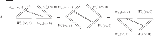
(a)

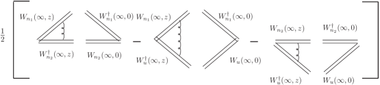
(b)

Figure 1: One-loop graphs for the soft subtraction factor in Eq. (2.1).

It is a crucial criterion that the linear divergence proportional to the length of Wilson lines should cancel in factorization-compatible definitions of a TMD wave function, leading to one of the key requirements for the construction of the soft subtraction factor. The soft factor is designed in the way that the rapidity divergences associated with the gauge vector $n_{1}$ cancel between $S(z;y_{1},y_{2})$ and $S(z;y_{1},y_{u})$, the pinched singularities in the self-energy corrections to the Wilson lines in $n_{2}$, mentioned above, cancel between $S(z;y_{1},y_{2})$ and $S(z;y_{2},y_{u})$, and the rapidity divergences in the un-subtracted wave function are cancelled by $S(z;y_{1},y_{u})$ and $S(z;y_{2},y_{u})$ in the limit $y_{u}\to-\infty$. These cancellations are easily understood from the typical one-loop diagrams for the soft factor in Fig. 1. As to the order of taking limits of various regulators, the prescription is as follows: (a) Take the trivial limit $L\to\infty$ for the length of the Wilson links; (b) Compute the un-subtracted wave function and the soft functions in $D=4-2\,\epsilon$ dimensions; (c) Take the limits of infinite Wilson-line rapidities $y_{1}\to+\infty$ and $y_{u}\to-\infty$; (d) Add the ultraviolet counterterms and remove the ultraviolet regulator by setting $\epsilon\to 0$. Detailed discussions on the exchange of the above limits can be found in Ref. [31].

Figure 1(a) yields the integral

$$S_{a}^{(1)}(k_{+}^{\prime},k_{T}^{\prime},y_{2})=-g_{s}^{2}\,C_{F}\,\mu^{2\epsilon}\,\int\frac{dl_{+}}{2\pi}\int\frac{d^{2-2\epsilon}l_{T}}{(2\pi)^{2-2\epsilon}}\,\,\,\delta(k_{+}^{\prime}-k_{+}-l_{+})\,\delta({\bf k}_{T}^{\prime}-{\bf k}_{T}-{\bf l}_{T})$$

$$\times\left[\frac{\theta(l_{+})\,\theta({\bar{k}}_{+}-l_{+})}{l_{+}+i0}-\frac{\theta(-l_{+})\,\theta(l_{+}+k_{+})}{l_{+}+i0}\right]\frac{1}{l_{T}^{2}+2\,e^{-2y_{2}}\,l_{+}^{2}+m_{g}^{2}-i0}\,,$$ (5)

where $k_{+}^{(\prime)}$ and ${\bf k}_{T}^{(\prime)}$ denote the plus and transverse components of the quark momentum before (after) the gluon emission for the partonic configuration $|u(k)\,\bar{d}(p-k)\rangle$ in the Fock-state expansion of $|\pi^{+}(p)\rangle$, and the shorthand notation ${\bar{k}}_{+}^{(\prime)}=p_{+}-k_{+}^{(\prime)}$ has been employed. The gluon mass $m_{g}$ regularizes the soft divergence to be cancelled by the contribution from Fig. 1(b),

$$S_{b}^{(1)}(k_{+}^{\prime},k_{T}^{\prime},y_{2})=g_{s}^{2}\,C_{F}\,\mu^{2\epsilon}\,\int\frac{dl_{+}}{2\pi}\int\frac{d^{2-2\epsilon}l_{T}}{(2\pi)^{2-2\epsilon}}\,\,\delta(k_{+}-k_{+}^{\prime})\,\delta({\bf k}_{T}-{\bf k}_{T}^{\prime})$$

$$\times\left[\frac{\theta(l_{+})}{l_{+}+i0}-\frac{\theta(-l_{+})}{l_{+}+i0}\right]\,\frac{1}{l_{T}^{2}+2\,e^{-2y_{2}}\,l_{+}^{2}+m_{g}^{2}-i0}\,.$$ (6)

The one-loop integrals for the un-subtracted TMD wave function from Fig. 2 are written as

$$\phi_{a}^{C(1)}(k_{+}^{\prime},k_{T}^{\prime}) = -g_{s}^{2}\,C_{F}\,\mu^{2\epsilon}\,\int_{-{\bar{k}}_{+}}^{0}\frac{dl_{+}}{2\pi}\int\frac{d^{2-2\epsilon}l_{T}}{(2\pi)^{2-2\epsilon}}\,\delta(k_{+}^{\prime}-k_{+}+l_{+})\,\delta({\bf k}_{T}^{\prime}-{\bf k}_{T}+{\bf l}_{T})$$

$$\times\frac{1}{l_{+}+i0}\,\frac{1}{l_{T}^{2}-{l_{+}\over l_{+}+{\bar{k}}_{+}}\,\left({\bf l}_{T}-{\bf k}_{T}\right)^{2}+i0}\,,$$

$$\phi_{c}^{C(1)}(k_{+}^{\prime},k_{T}^{\prime}) = -ig_{s}^{2}\,C_{F}\,(2-2\epsilon)\,\mu^{2\epsilon}\,\int\frac{d^{4-2\epsilon}l}{(2\pi)^{4-2\epsilon}}\,\,\delta(k_{+}^{\prime}-k_{+}+l_{+})\,\delta({\bf k}_{T}^{\prime}-{\bf k}_{T}+{\bf l}_{T})$$

$$\times\frac{({\bf k}_{T}-{\bf l}_{T})^{2}}{[(p-k+l)^{2}+i0][(k-l)^{2}+i0][l^{2}+i0]}\,,$$

$$\phi_{e}^{C(1)}(k_{+}^{\prime},k_{T}^{\prime}) = g_{s}^{2}\,C_{F}\,\mu^{2\epsilon}\,\int_{-{\bar{k}}_{+}}^{0}\frac{dl_{+}}{2\pi}\int\frac{d^{2-2\epsilon}l_{T}}{(2\pi)^{2-2\epsilon}}\,\delta(k_{+}-k_{+}^{\prime})\,\delta({\bf k_{T}}-{\bf k_{T}^{\prime}})$$

$$\times\frac{1}{l_{+}+i0}\,\frac{1}{l_{T}^{2}-{l_{+}\over l_{+}+{\bar{k}}_{+}}\,\left({\bf l}_{T}-{\bf k}_{T}\right)^{2}+i0}\,,$$

$$\phi_{b\,(d)}^{C(1)}(k_{+}^{\prime},k_{T}^{\prime}) = \phi_{a\,(e)}^{(1)}\,\left[k_{+}^{(\prime)}\to{\bar{k}}_{+}^{(\prime)}\,,{\bf k}_{T}^{(\prime)}\to-{\bf k}_{T}^{(\prime)}\right].$$ (7)

The contribution from Fig. 2(f) vanishes in Feynman gauge due to the light-like gauge link in the direction of $n_{-}$, and it is cancelled by those of the corresponding diagrams from $S(z;y_{1},y_{u})$ and $S(z;y_{2},y_{u})$ in arbitrary gauge as stated before.

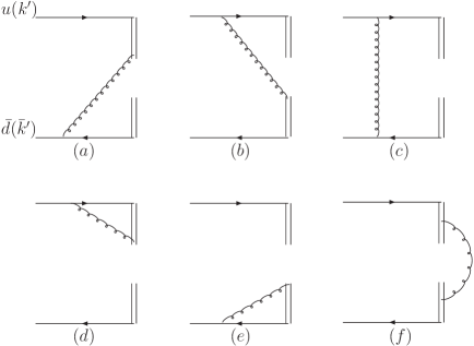
Figure 2: One-loop graphs for the un-subtracted TMD wave function.

To illustrate the cancellations of the rapidity singularities from $l_{+}=0$ and of the pinched singularities from the Wilson-line self-energy corrections to the pion wave function in Eq. (1), we present the explicit expression for the sum of $\phi_{a}^{C(1)}$, $\phi_{b}^{C(1)}$, and $S_{a}^{(1)}$,

$$\phi_{a}^{C(1)}+\phi_{b}^{C(1)}+S_{a}^{(1)}=-\frac{\alpha_{s}\,C_{F}}{2\pi}\,D_{red}\,\,\delta(k_{+}-k_{+}^{\prime})\,\delta({\bf k}_{T}-{\bf k}_{T}^{\prime})$$

$$-\frac{\alpha_{s}\,C_{F}}{2\pi^{2}}\,\bigg{\{}\frac{\theta(k_{+}^{\prime}-k_{+})\,\theta({\bar{k}}_{+}^{\prime})}{(k_{+}-k_{+}^{\prime})\left[\left({\bf k}_{T}^{\prime}-{\bf k}_{T}\right)^{2}-{k_{+}-k_{+}^{\prime}\over p_{+}-k_{+}^{\prime}}{\bf k}_{T}^{\prime\,\,2}\right]}$$

$$-\frac{\theta(k_{+}^{\prime}-k_{+})\,\theta({\bar{k}}_{+}^{\prime})}{(k_{+}-k_{+}^{\prime})\left[\left({\bf k}_{T}^{\prime}-{\bf k}_{T}\right)^{2}+2\,e^{-2y_{2}}\,(k_{+}^{\prime}-k_{+})^{2}\right]}$$

$$+\frac{\theta(k_{+}^{\prime})\,\theta(k_{+}-k_{+}^{\prime})}{(k_{+}^{\prime}-k_{+})\left[\left({\bf k}_{T}^{\prime}-{\bf k}_{T}\right)^{2}-{k_{+}^{\prime}-k_{+}\over k_{+}^{\prime}}{\bf k}_{T}^{\prime\,\,2}\right]}$$

$$-\frac{\theta(k_{+}^{\prime})\,\theta(k_{+}-k_{+}^{\prime})}{(k^{\prime}_{+}-k_{+})\left[\left({\bf k}_{T}^{\prime}-{\bf k}_{T}\right)^{2}+2\,e^{-2y_{2}}\,(k_{+}^{\prime}-k_{+})^{2}\right]}\bigg{\}}_{\oplus}\,,$$ (8)

with the factor

$$D_{red} = 2\left(\frac{1}{\hat{\epsilon}}+\ln{\mu^{2}\over k_{T}^{2}}\right)+\ln^{2}\left({k_{+}\over m_{g}}\right)+\ln^{2}\left({\bar{k}_{+}\over m_{g}}\right)+\ln\left({k_{T}^{2}\over m_{g}^{2}}\right)\cdot\ln\left({k_{T}^{2}\over k_{+}\bar{k}_{+}}\right)$$ (9)

$$-\frac{1}{2}\ln^{2}\left(2\,e^{-2y_{2}}\right)-\ln\left(2\,e^{-2y_{2}}\right)\cdot\ln\left({k_{+}\bar{k}_{+}\over m_{g}^{2}}\right)+4-{\pi^{2}\over 6}\,,$$

and $1/\hat{\epsilon}\equiv 1/\epsilon-\gamma_{E}+\ln(4\pi)$. The “$\oplus$” subtraction is defined as

$$\left[f(k_{+},k^{\prime}_{+},{\bf k}_{T},{\bf k}_{T}^{\prime})\right]_{\oplus}=f(k_{+},k^{\prime}_{+},{\bf k}_{T},{\bf k}_{T}^{\prime})-\delta(k_{+}-k_{+}^{\prime})\,\delta({\bf k}_{T}-{\bf k}_{T}^{\prime})$$

$$\,\times\int_{-\infty}^{+\infty}dq_{+}\int_{-\infty}^{+\infty}d^{2-2\epsilon}q_{T}\,f(k_{+},q_{+},{\bf k}_{T},{\bf q}_{T})\,.$$ (10)

It is evident that Eq. (8) is free of the rapidity divergence from $k_{+}=k^{\prime}_{+}$, and contains only the ordinary logarithmic soft divergence regularized by the gluon mass. This logarithmic divergence is cancelled precisely by that in the sum of $\phi_{d}^{C(1)}$, $\phi_{e}^{C(1)}$, and $S_{b}^{(1)}$,

$$\phi_{d}^{C(1)}+\phi_{e}^{C(1)}+S_{b}^{(1)} = \frac{\alpha_{s}\,C_{F}}{2\pi}\bigg{\{}D_{red}\,+{\Gamma(\epsilon)\over 2\,\epsilon}\,\left(2\,e^{-2y_{2}}\right)^{-\epsilon}\left[\left(\frac{4\,\pi\,\mu^{2}}{k_{+}^{2}}\right)^{\epsilon}+\left(\frac{4\,\pi\,\mu^{2}}{\bar{k}^{2}_{+}}\right)^{\epsilon}\right]\bigg{\}}$$ (11)

$$\times\delta(k_{+}-k_{+}^{\prime})\,\delta({\bf k}_{T}-{\bf k}_{T}^{\prime})\,.$$

Evaluation of Fig. 2(c) gives

$$\phi_{c}^{C(1)}(k_{+}^{\prime},k_{T}^{\prime}) = -\frac{\alpha_{s}\,C_{F}}{4\pi}\left[\frac{1}{\hat{\epsilon}}+\ln{\mu^{2}\over k_{T}^{2}}+1\right]\delta(k_{+}-k_{+}^{\prime})\,\delta({\bf k}_{T}-{\bf k}_{T}^{\prime})-\frac{\alpha_{s}\,C_{F}}{2\pi^{2}}\,{1\over p_{+}}\,$$ (12)

$$\times\bigg{\{}\frac{\theta(k_{+}^{\prime})\,\theta(k_{+}-k_{+}^{\prime})}{\left({\bf k}_{T}^{\prime}-{\bf k}_{T}\right)^{2}+{k_{+}-k_{+}^{\prime}\over k_{+}^{\prime}}{\bf k}_{T}^{\prime\,\,2}}\,+\frac{\theta(k_{+}^{\prime}-k_{+})\,\theta({\bar{k}}_{+}^{\prime})}{\left({\bf k}_{T}^{\prime}-{\bf k}_{T}\right)^{2}+{k^{\prime}_{+}-k_{+}\over p_{+}-k_{+}^{\prime}}{\bf k}_{T}^{\prime\,\,2}}\bigg{\}}_{\oplus}\,,$$

which does not contain a soft divergence.

We then obtain the next-to-leading-order (NLO) TMD pion wave function from Fig. 1 and Fig. 2,

$$\phi^{C(1)}(k_{+}^{\prime},k_{T}^{\prime},y_{2}) = -\frac{\alpha_{s}\,C_{F}}{4\pi}\bigg{\{}\frac{1}{\hat{\epsilon}}+\ln{\mu^{2}\over k_{T}^{2}}+1-{\Gamma(\epsilon)\over\,\epsilon}\left(2\,e^{-2y_{2}}\right)^{-\epsilon}\left[\left(\frac{4\,\pi\,\mu^{2}}{k_{+}^{2}}\right)^{\epsilon}+\left(\frac{4\,\pi\,\mu^{2}}{\bar{k}^{2}_{+}}\right)^{\epsilon}\right]\bigg{\}}$$

$$\times\delta(k_{+}-k_{+}^{\prime})\,\delta({\bf k}_{T}-{\bf k}_{T}^{\prime})-\frac{\alpha_{s}\,C_{F}}{2\pi^{2}}\,\bigg{\{}\frac{\theta(k_{+}^{\prime}-k_{+})\,\theta({\bar{k}}_{+}^{\prime})}{(k_{+}-k_{+}^{\prime})\left[\left({\bf k}_{T}^{\prime}-{\bf k}_{T}\right)^{2}-{k_{+}-k_{+}^{\prime}\over p_{+}-k_{+}^{\prime}}{\bf k}_{T}^{\prime\,\,2}\right]}$$

$$-\frac{\theta(k_{+}^{\prime}-k_{+})\,\theta({\bar{k}}_{+}^{\prime})}{(k_{+}-k_{+}^{\prime})\left[\left({\bf k}_{T}^{\prime}-{\bf k}_{T}\right)^{2}+2\,e^{-2y_{2}}\,(k_{+}^{\prime}-k_{+})^{2}\right]}$$

$$+\frac{\theta(k_{+}^{\prime})\,\theta(k_{+}-k_{+}^{\prime})}{(k_{+}^{\prime}-k_{+})\left[\left({\bf k}_{T}^{\prime}-{\bf k}_{T}\right)^{2}-{k_{+}^{\prime}-k_{+}\over k_{+}^{\prime}}{\bf k}_{T}^{\prime\,\,2}\right]}$$

$$-\frac{\theta(k_{+}^{\prime})\,\theta(k_{+}-k_{+}^{\prime})}{(k^{\prime}_{+}-k_{+})\left[\left({\bf k}_{T}^{\prime}-{\bf k}_{T}\right)^{2}+2\,e^{-2y_{2}}\,(k_{+}^{\prime}-k_{+})^{2}\right]}$$

$$+\frac{\theta(k_{+}^{\prime})\,\theta(k_{+}-k_{+}^{\prime})}{p_{+}\left[\left({\bf k}_{T}^{\prime}-{\bf k}_{T}\right)^{2}+{k_{+}-k_{+}^{\prime}\over k_{+}^{\prime}}{\bf k}_{T}^{\prime\,\,2}\right]}+\frac{\theta(k_{+}^{\prime}-k_{+})\,\theta({\bar{k}}_{+}^{\prime})}{p_{+}\left[\left({\bf k}_{T}^{\prime}-{\bf k}_{T}\right)^{2}+{k^{\prime}_{+}-k_{+}\over p_{+}-k_{+}^{\prime}}{\bf k}_{T}^{\prime\,\,2}\right]}\bigg{\}}_{\oplus}\,,$$

indicating that the remaining infrared divergence in the NLO pion wave function is the collinear one regularized by the parton virtuality $k_{T}^{2}$. To validate the $k_{T}$ factorization theorem for the pion transition form factor, we show the infrared finiteness of the hard kernel obtained from matching the QCD diagrams onto the effective diagrams $\phi^{C(1)}$. The collinear logarithm $\ln k_{T}^{2}$ is extracted explicitly from the convolution of the NLO pion wave function with the leading-order hard kernel $H^{(0)}$ of the pion transition form factor:

$$\int_{-\infty}^{+\infty}dk_{+}^{\prime}\int_{-\infty}^{+\infty}d^{2-2\epsilon}k_{T}^{\prime}\,\,\phi^{C(1)}(k_{+}^{\prime},k_{T}^{\prime},y_{2})\,H^{(0)}(k_{+}^{\prime},k_{T}^{\prime})$$

$$=-{\alpha_{s}\,C_{F}\over 4\pi}\,\left[\ln\left({k_{+}\over p_{+}}\right)+2\right]\,\ln k_{T}^{2}\,H^{(0)}(k_{+},k_{T})+\cdots\,,$$ (14)

where the ellipsis represents the terms independent of $\ln k_{T}^{2}$ at leading power. It is indeed the case that Eq. (14) cancels the $\ln k_{T}^{2}$ term in the one-loop QCD diagrams for the pion transition form factor given by Eq. (20) of [19], as those from the self-energy corrections to the external quarks are excluded.

3 TMD wave functions with non-dipolar Wilson lines

In view of the complicated structure of the soft subtraction in Eq. (1), it is in demand to construct factorization-compatible definitions of a TMD wave function with simper subtraction factors for practical calculations. We start with the un-subtracted TMD wave function in Eq. (1), where the future-pointing or past-pointing light-like Wilson links have been appropriately chosen to facilitate the $k_{T}$ factorization by avoiding the Glauber region. Certainly, the Glauber region does not exist in a simple process [39, 40] like the pion transition form factor considered here. The Wilson links are then rotated away from the light cone, as done in [26, 31], to regularize the rapidity divergence. The key of our proposal is that the two pieces of Wilson links are rotated into different directions, such that the pinched singularity in Wilson-line self-energy corrections, arising from the integrand $[(n\cdot l+i0)(n\cdot l-i0)]^{-1}$, is alleviated into $[(n\cdot l+i0)(n^{\prime}\cdot l-i0)]^{-1}$. Hence, the soft subtraction required to remove this ordinary infrared singularity with the non-dipolar Wilson links is simpler. The technique of rotating the Wilson links has been also employed to derive various resummations for a TMD wave function [41]. We then need to examine whether the above rotation of Wilson links would change the collinear logarithms $\ln k_{T}^{2}$, which have been absorbed into the un-subtracted TMD wave function. As postulated in the Introduction and demonstrated by explicit calculations below, the new definition reproduces the correct collinear logarithms.

We consider the case with two orthogonal pieces of off-light-cone Wilson links:

$$\phi^{W}(k_{+}^{\prime},k_{T}^{\prime},y_{2})=\int\frac{dz_{-}}{2\pi}\int\frac{d^{2}z_{T}}{(2\pi)^{2}}\,e^{i(k_{+}^{\prime}z_{-}-k_{T}^{\prime}z_{T})}\,$$

$$\times\langle 0|\bar{d}(0)W^{{\dagger}}_{n_{2}}(+\infty,0)\!\not n_{-}\,\gamma_{5}\,W_{v}(\infty,z)\,u(z)|\pi^{+}(p)\rangle\,,$$ (15)

where the gauge vectors $n_{2}$ and $v=(-e^{y_{2}},e^{-y_{2}},\bf{0_{T}})$ are introduced into the un-subtracted wave function. Compared to Eq. (1), the vector $u$ in the first (second) piece of Wilson links $W_{u}$ ($W^{{\dagger}}_{u}$) has been rotated slightly into the space-like (time-like) direction $v$ ($n_{2}$) with large $-y_{2}$. The orthogonality $n_{2}\cdot v=0$ implies that the contribution of Fig 2(f) vanishes in Feynman gauge, and that a soft subtraction factor is not required in this definition. That is, Eq. (15) will not cause double counting of soft gluons, when it is implemented into a process more complicated than the pion transition form factor, which demands soft-gluon factorization.

Computing all the one-loop graphs in Fig. 2 according to Eq. (15), we derive

$${\phi}^{W(1)}_{a}(k_{+}^{\prime},k_{T}^{\prime},y_{2}) = {\alpha_{s}\,C_{F}\over 4\,\pi}\,\bigg{[}\ln^{2}\left({2\,e^{-2y_{2}}\bar{k}_{+}^{2}\over k_{T}^{2}}\right)-2\,\ln\left({2\,e^{-2y_{2}}\bar{k}_{+}^{2}\over k_{T}^{2}}\right)\bigg{]}\delta(k_{+}-k_{+}^{\prime})\,\delta({\bf k}_{T}-{\bf k}_{T}^{\prime})\,$$

$$+{\alpha_{s}\,C_{F}\over\pi^{2}}\,\bigg{\{}\frac{\theta(k_{+}^{\prime}-k_{+})\,\theta(\bar{k}_{+}^{\prime})}{{({\bf k}_{T}^{\prime}-{\bf k}_{T})}^{2}-\left({k_{+}-k_{+}^{\prime}\over p_{+}-k_{+}^{\prime}}\right){\bf k}_{T}^{\prime\,\,2}}\frac{e^{-2y_{2}}\,(k_{+}-k_{+}^{\prime})}{{({\bf k}_{T}^{\prime}-{\bf k}_{T})}^{2}-2\,e^{-2y_{2}}\,(k_{+}^{\prime}-k_{+})^{2}}\bigg{\}}_{\oplus}\,,$$

$${\phi}^{W(1)}_{b}(k_{+}^{\prime},k_{T}^{\prime},y_{2}) = {\alpha_{s}\,C_{F}\over 4\,\pi}\,\bigg{[}\ln^{2}\left({2\,e^{-2y_{2}}k_{+}^{2}\over k_{T}^{2}}\right)-2\,\ln\left({2\,e^{-2y_{2}}k_{+}^{2}\over k_{T}^{2}}\right)+\pi^{2}\bigg{]}\delta(k_{+}-k_{+}^{\prime})\,\delta({\bf k}_{T}-{\bf k}_{T}^{\prime})\,$$

$$-{\alpha_{s}\,C_{F}\over\pi^{2}}\,\bigg{\{}\frac{\theta({k}_{+}^{\prime})\,\theta(k_{+}-k_{+}^{\prime})}{{({\bf k}_{T}^{\prime}-{\bf k}_{T})}^{2}-\left({k_{+}^{\prime}-k_{+}\over k_{+}^{\prime}}\right){\bf k}_{T}^{\prime\,\,2}}\frac{e^{-2y_{2}}\,(k_{+}^{\prime}-k_{+})}{{({\bf k}_{T}^{\prime}-{\bf k}_{T})}^{2}+2\,e^{-2y_{2}}\,(k_{+}^{\prime}-k_{+})^{2}}\bigg{\}}_{\oplus}\,,$$

$${\phi}^{W(1)}_{c}(k_{+}^{\prime},k_{T}^{\prime},y_{2}) = \phi^{C(1)}_{c}(k_{+}^{\prime},k_{T}^{\prime})\,,$$

$${\phi}^{W(1)}_{d}(k_{+}^{\prime},k_{T}^{\prime},y_{2}) = {\alpha_{s}\,C_{F}\over 4\,\pi}\,\bigg{[}{1\over\hat{\epsilon}}+\ln\left({\mu^{2}\over k_{T}^{2}}\right)-\ln^{2}\left({2\,e^{-2y_{2}}k_{+}^{2}\over k_{T}^{2}}\right)+\ln\left({2\,e^{-2y_{2}}k_{+}^{2}\over k_{T}^{2}}\right)-{\pi^{2}\over 3}+2\bigg{]}$$

$$\times\delta(k_{+}-k_{+}^{\prime})\,\delta({\bf k}_{T}-{\bf k}_{T}^{\prime})\,,$$

$${\phi}^{W(1)}_{e}(k_{+}^{\prime},k_{T}^{\prime},y_{2}) = {\phi}^{W(1)}_{d}(k_{+}^{\prime},k_{T}^{\prime},y_{2})\big{|}_{k_{+}\to\bar{k}_{+}}-\pi^{2}\,\delta(k_{+}-k_{+}^{\prime})\,\delta({\bf k}_{T}-{\bf k}_{T}^{\prime})\,.$$ (16)

It is trivial to confirm that the sum of all the graphs in Fig. 2 reproduces the $\ln k_{T}^{2}$ term the same as in Eq. (14), namely, the same as in [19].

4 Equivalence of TMD Definitions

We first point out that the TMD wave functions in Eqs. (1) and (15) approach to the naive definition

$$\phi^{N}(k_{+}^{\prime},k_{T}^{\prime},y_{2}) = \lim_{y_{u}\to-\infty}\,\,\int\frac{dz_{-}}{2\pi}\int\frac{d^{2}z_{T}}{(2\pi)^{2}}\,e^{i(k_{+}^{\prime}z_{-}-k_{T}^{\prime}z_{T})}\,$$ (17)

$$\times\langle 0|\bar{d}(0)W^{{\dagger}}_{u}(+\infty,0)\!\not n_{-}\,\gamma_{5}\,W_{u}(+\infty,z)\,u(z)|\pi^{+}(p)\rangle\,,$$

in the limit of vanishing infrared regulators. It is easy to see $S(z;y_{2},y_{u})=1$ following Eq. (2) and $S(z;y_{1},y_{2})=S(z;y_{1},y_{u})$ for the rapidities $y_{2}=y_{u}$, so that Eq. (1) reduces to Eq. (17) as $y_{2}=y_{u}\to-\infty$. In the same limit both the gauge vectors $n_{2}$ and $v$ approach to $u$, and Eq. (15) also reduces to Eq. (17). The infinitesimal components $v^{+}=-e^{y_{u}}$ and $u^{+}=e^{y_{u}}$, being opposite in sign, serve as regulators for the rapidity divergences. It has been known that the regularization of rapidity divergences, which do not exist in QCD diagrams, is a matter of factorization schemes [24]. That is, Eq. (15) collects the same collinear divergences as Eq. (1) which are associated with the initial pion in the limit $y_{2}=y_{u}\to-\infty$.

We then demonstrate that Eqs. (1) and (15) collect the same collinear divergences for arbitrary rapidity $y_{2}$ as well. The TMD wave function in Eq. (1) depends on the Lorentz invariants $p\cdot n_{2}$, $n_{2}^{2}$, and $k^{2}=-k_{T}^{2}$ formed by the vectors $p$, $k$ and $n_{2}$. An infrared divergence is regularized by the parton virtuality $k^{2}$ into $\ln k_{T}^{2}$ in $k_{T}$ factorization as indicated by the one-loop result in Eq. (14). Because the argument of a logarithm is dimensionless, $k_{T}$ appears in the ratio $p_{+}^{2}/k_{T}^{2}$ or $\mu^{2}/k_{T}^{2}$. Equations (1) and (15) contain the same infrared logarithm $\ln(\mu^{2}/k_{T}^{2})$, which is generated by a loop correction without involving the Wilson links. Therefore, we just focus on the logarithm $\ln(p_{+}^{2}/k_{T}^{2})$ in the two TMD definitions. Since the Feynman rule $n_{2}^{\mu}/n_{2}\cdot l$ associated with the Wilson link is scale invariant in $n_{2}$, $p_{+}^{2}/k_{T}^{2}$ must arise from the ratio $(p\cdot n_{2})^{2}/(n_{2}^{2}k^{2})\propto(p_{+}^{2}e^{-2y_{2}})/k_{T}^{2}$ for Eq. (1). Equation (15) depends on the additional vector $v$ but with $n_{2}\cdot v=0$. The arguments of its infrared logarithms are then given by $(p\cdot n_{2})^{2}/(n_{2}^{2}k^{2})$ and $(p\cdot v)^{2}/(v^{2}k^{2})$, which are both proportional to $(p_{+}^{2}e^{-2y_{2}})/k_{T}^{2}$. To study the infrared behaviors of Eqs. (1) and (15) for arbitrary $y_{2}$, we vary $y_{2}$ below.

Consider the derivative

$$\frac{d}{dy_{2}}\phi^{C}=\frac{n_{2}^{2}}{2p\cdot n_{2}}p^{\alpha}\frac{d}{dn_{2}^{\alpha}}\phi^{C}\,,$$ (18)

which is a straightforward consequence of the chain rule [42]. The differentiation $d/dn_{2}^{\alpha}$ applies to the Wilson links in the direction of $n_{2}$, leading to the Feynman rule

$$\frac{n_{2}^{2}}{2p\cdot n_{2}}p^{\alpha}\frac{d}{dn_{2}^{\alpha}}\frac{n_{2}^{\mu}}{n_{2}\cdot l}=\frac{\hat{n}_{2}^{\mu}}{n_{2}\cdot l}\,,$$ (19)

with the special vertex [43]

$$\hat{n}_{2}^{\mu}=\frac{n_{2}^{2}}{2p\cdot n_{2}}\left(p^{\mu}-\frac{p\cdot l}{n_{2}\cdot l}n_{2}^{\mu}\right)\,.$$ (20)

Equation (18) then yields

$$\frac{d}{dy_{2}}\phi^{C}=\lim_{\begin{subarray}{c}y_{1}\to+\infty\\ y_{u}\to-\infty\end{subarray}}\,\frac{1}{2}\left[\frac{S^{\,\prime}(z;y_{1},y_{2})}{S(z;y_{1},y_{2})}-\frac{S^{\,\prime}(z;y_{2},y_{u})}{S(z;y_{2},y_{u})}\right]\phi^{C}\,,$$ (21)

in coordinate space, where the primed soft functions $S^{\,\prime}$ include the diagrams from those in the soft functions $S$, with an original vertex $n_{2}^{\mu}$ being replaced by a special vertex $\hat{n}_{2}^{\mu}$ on the Wilson links in the direction of $n_{2}$.

In the leading-power approximation, the accuracy at which Eq. (1) is defined, the diagrams in $S^{\,\prime}(z;y_{1},y_{2})$ are organized into a product of the soft function $S(z;y_{1},y_{2})$ with a soft kernel $K(z;y_{1},y_{2})$ following the argument in [21, 43]. The soft kernel $K(z;y_{1},y_{2})$ contains the same set of diagrams as the soft function $S(z;y_{1},y_{2})$ at each order of the strong coupling constant, but with a special vertex on the Wilson links in the direction of $n_{2}$ [21, 43]. Similarly, $S^{\,\prime}(z;y_{2},y_{u})$ is expressed as a product of $S(z;y_{2},y_{u})$ and $K(z;y_{2},y_{u})$ at leading power, so Eq. (21) is simplified into

$$\frac{d}{dy_{2}}\phi^{C}=\lim_{\begin{subarray}{c}y_{1}\to+\infty\\ y_{u}\to-\infty\end{subarray}}\,\frac{1}{2}\left[K(z;y_{1},y_{2})-K(z;y_{2},y_{u})\right]\phi^{C}\,.$$ (22)

Because the special vertex suppresses collinear dynamics [21, 43], the soft kernels $K(z;y_{1},y_{2})$ and $K(z;y_{2},y_{u})$ collect only the single logarithms $\ln(n_{2}\cdot n_{1})$ and $\ln(n_{2}\cdot u)$, respectively. With the relation between the infrared logarithms in the limit $y_{1}=-y_{u}\to\infty$, $\ln(n_{2}\cdot u)=-\ln(n_{2}\cdot n_{1})$, which holds for arbitrary finite $y_{2}$, we have $K(z;y_{1},y_{2})\approx-K(z;y_{2},y_{u})$ up to different infrared finite pieces, and

$$\frac{d}{dy_{2}}\phi^{C}\approx\lim_{y_{1}\to+\infty}\,K(z;y_{1},y_{2})\phi^{C}\,,$$ (23)

from Eq. (22).

Both the variations with respect to $n_{2}$ and $v$ are related to the variation of $y_{2}$ via the chain rule, so the above derivation applies to the TMD wave function in Eq. (15). We obtain

$$\frac{d}{dy_{2}}\phi^{W}\equiv\left[\frac{n_{2}^{2}}{2p\cdot n_{2}}p^{\alpha}\frac{d}{dn_{2}^{\alpha}}+\frac{v^{2}}{2p\cdot v}p^{\alpha}\frac{d}{dv^{\alpha}}\right]\phi^{W},$$ (24)

where the first (second) term on the right hand side includes the diagrams from those in $\phi^{W}$, with an original vertex $n_{2}^{\mu}$ ($v^{\mu}$) being replaced by a special vertex $\hat{n}_{2}^{\mu}$ ($\hat{v}^{\mu}$) on the Wilson link in the direction of $n_{2}$ ($v$). The definition of the special vertex $\hat{v}^{\mu}$ is similar to $\hat{n}_{2}^{\mu}$ in Eq. (20) but with the vector $n_{2}$ being replaced by $v$. A subset of diagrams, in which the gluon emitted by the special vertex $\hat{n}_{2}^{\mu}$ ($\hat{v}^{\mu}$) carries a small momentum, is factorized out of the first (second) derivative in Eq. (24). The resultant soft kernel is composed of a pair of Wilson links in the direction of $n_{1}$, which are collimated to the initial quarks in the limit $y_{1}\to\infty$ [21, 43], a Wilson link in the direction of $n_{2}$, and a Wilson link in the direction of $v$. A special vertex $\hat{n}_{2}^{\mu}$ ($\hat{v}^{\mu}$) appears on the Wilson link in the direction of $n_{2}$ ($v$) in the first (second) soft kernel. Due to the suppression from the special vertices on collinear dynamics, the first and second soft kernels collect only the single logarithms $\ln(n_{2}\cdot n_{1})$ and $\ln(v\cdot n_{1})$, respectively. It is obvious that these two logarithms are equal in the limit $y_{1}\to\infty$, and can be combined into the soft kernel $K(z;y_{1},y_{2})$.

Note that the Wilson links along $n_{2}$ and $v$ attach to the energetic quarks, instead of to other Wilson links. In addition to the soft kernel $K$ factorized above, another subset of diagrams, in which the gluon emitted by the special vertex and attaching to the quark line carries a large (but not collinear) momentum, can also be factorized [42]. This factorization follows the argument in [21], and the resultant hard kernel $G(z,y_{2})$ contains a special vertex on the Wilson link in the direction of $n_{2}$ or of $v$. Hence, the two terms in Eq. (24) are summed into the product

$$\frac{d}{dy_{2}}\phi^{W}=\lim_{y_{1}\to+\infty}\,[K(z;y_{1},y_{2})+G(z,y_{2})]\phi^{W}.$$ (25)

The functions $K$ and $G$ correspond to the known soft and hard kernels in the typical Sudakov resummation [42], both of which can be evaluated order by order according to their definitions described above, with their one-loop expressions being found in [21]. We have confirmed that the resultant rapidity evolution equation is the same as the one derived in [19] in the small $k_{+}^{\prime}$ limit, namely, in the so-called small $x$ limit, where the $k_{T}$ factorization theorem is an appropriate theoretical framework for exclusive processes. Note that $K$ and $G$ depend on a factorization scale $\mu$, which cancels in their sum $K+G$. The $\mu$-dependent kernel in Eq. (23) was also observed in the rapidity evolution kernel for the TMD fragmentation function (see Eq. (13.55) of [31]), and calls for a simultaneous treatment of the rapidity and factorization-scale evolutions.

We have shown that $\phi^{C}$ and $\phi^{W}$ reduce to the naive TMD wave function as $y_{2}=y_{u}\to-\infty$. Apparently, the hard kernel $G$ does not depend on the infrared logarithm $\ln k_{T}$, and can be regarded as a finite piece. Equations (23) and (25), governed by the identical soft kernel $K$, then imply that $\phi^{C}$ and $\phi^{W}$ have the same infrared logarithms at leading power for arbitrary $y_{2}$. However, they are established in different factorization schemes represented by the infrared finite piece $G$. We claim that the two TMD definitions considered in this work are equivalent in the infrared behavior at all orders of the strong coupling constant, and supersede the one presented in [21].

5 Conclusion

In this paper we have first investigated the infrared behavior of a TMD pion wave function with the dipolar Wilson links and the complicated soft subtraction, which was originally developed for a TMD parton density. The TMD wave-function definition with non-dipolar off-light-cone Wilson links was then proposed, which was shown to realize the $k_{T}$ factorization of hard exclusive processes appropriately as well. It is free of the rapidity divergence and of the pinched singularity in the self-energy correction to the dipolar Wilson lines, and demands simpler soft subtraction. We have illustrated its property by considering the special case with two orthogonal gauge vectors, for which the soft subtraction is not needed in Feynman gauge. It was explicitly demonstrated at one-loop level that this definition yields the collinear logarithms $\ln k_{T}^{2}$ the same as in the one with the dipolar gauge links, which cancel those in the QCD diagrams, albeit with a distinct ultraviolet structure. We then illustrated the equivalence of the two definitions by showing that both of them reduce to the naive TMD wave function as the non-light-like Wilson links approach to the light cone, and that their evolutions with the rapidity of the non-light-like Wilson links are governed by the same soft kernel. In this reasoning it also became clear that the two TMD wave functions were established in different factorization schemes.

As stressed at the beginning of Sec. 3, we started with the un-subtracted TMD wave function in Eq. (1), where the future-pointing or past-pointing light-like Wilson links have been appropriately chosen to facilitate the $k_{T}$ factorization by avoiding the Glauber region. Therefore, our proposal for a TMD wave function facilitates proofs of the $k_{T}$ factorization theorem for hard exclusive reactions, and derivations of their various evolution equations. It is then crucial to explore phenomenological consequences of applying the new TMD definition, which includes evolution effects, to $k_{T}$ factorization formulas for exclusive processes. It is straightforward to extend our proposal to the definition of the $B$ meson TMD wave functions in the heavy-quark effective theory, which will put the perturbative QCD factorization approach to exclusive $B$ meson decays on more solid ground. It is also of interest to examine the impact of the new TMD definition on polarized processes, for which Wilson-link interactions play an important role. We plan to study the above topics in future publications.

References

• [1] F. del Aguila and M. K. Chase, Nucl. Phys. B 193, 517 (1981).
• [2] E. Braaten, Phys. Rev. D 28, 524 (1983).
• [3] E. P. Kadantseva, S. V. Mikhailov and A. V. Radyushkin, Yad. Fiz.  44, 507 (1986) [Sov. J. Nucl. Phys.  44, 326 (1986)].
• [4] R. D. Field, R. Gupta, S. Otto and L. Chang, Nucl. Phys. B 186, 429 (1981).
• [5] E. Braaten and S. M. Tse, Phys. Rev. D 35, 2255 (1987).
• [6] B. Melic, B. Nizic and K. Passek, Phys. Rev. D 60, 074004 (1999) [hep-ph/9802204].
• [7] M. Beneke and T. Feldmann, Nucl. Phys. B 592, 3 (2001) [hep-ph/0008255].
• [8] M. Beneke, Y. Kiyo and D. S. Yang, Nucl. Phys. B 692, 232 (2004) [hep-ph/0402241].
• [9] M. Beneke and D. S. Yang, Nucl. Phys. B 736, 34 (2006) [hep-ph/0508250].
• [10] R. J. Hill, T. Becher, S. J. Lee and M. Neubert, JHEP 0407, 081 (2004) [hep-ph/0404217].
• [11] T. Becher and R. J. Hill, JHEP 0410, 055 (2004) [hep-ph/0408344].
• [12] I. I. Balitsky, V. M. Braun and A. V. Kolesnichenko, Nucl. Phys. B 312, 509 (1989).
• [13] V. M. Belyaev, A. Khodjamirian and R. Rückl, Z. Phys. C 60, 349 (1993) [hep-ph/9305348].
• [14] S. S. Agaev, V. M. Braun, N. Offen and F. A. Porkert, Phys. Rev. D 83, 054020 (2011) [arXiv:1012.4671 [hep-ph]].
• [15] V. M. Belyaev, V. M. Braun, A. Khodjamirian and R. Ruckl, Phys. Rev. D 51, 6177 (1995) [hep-ph/9410280].
• [16] A. Khodjamirian, C. Klein, T. Mannel and Y.-M. Wang, JHEP 1109, 106 (2011) [arXiv:1108.2971 [hep-ph]].
• [17] J. Collins, Int. J. Mod. Phys. Conf. Ser.  4, 85 (2011) [arXiv:1107.4123 [hep-ph]].
• [18] J. Collins, EPJ Web Conf.  85, 01002 (2015) [arXiv:1409.5408 [hep-ph]].
• [19] S. Nandi and H. n. Li, Phys. Rev. D 76, 034008 (2007) [arXiv:0704.3790 [hep-ph]].
• [20] H. n. Li and S. Mishima, Phys. Rev. D 80, 074024 (2009) [arXiv:0907.0166 [hep-ph]].
• [21] H. N. Li, Y. L. Shen and Y. M. Wang, JHEP 1401, 004 (2014) [arXiv:1310.3672 [hep-ph]]; Y. M. Wang, Int. J. Mod. Phys. Conf. Ser.  37 (2015) 1560049.
• [22] H. n. Li, Y. L. Shen, Y. M. Wang and H. Zou, Phys. Rev. D 83, 054029 (2011) [arXiv:1012.4098 [hep-ph]].
• [23] H. n. Li, Y. L. Shen and Y. M. Wang, Phys. Rev. D 85, 074004 (2012) [arXiv:1201.5066 [hep-ph]].
• [24] J. C. Collins, Acta Phys. Polon. B 34, 3103 (2003) [hep-ph/0304122].
• [25] A. Bacchetta, D. Boer, M. Diehl and P. J. Mulders, JHEP 0808, 023 (2008) [arXiv:0803.0227 [hep-ph]].
• [26] J. C. Collins and D. E. Soper, Nucl. Phys. B194, 445 (1982).
• [27] S. J. Brodsky, D. S. Hwang, B. Q. Ma and I. Schmidt, Nucl. Phys. B 593, 311 (2001) [hep-th/0003082].
• [28] I. O. Cherednikov and N. G. Stefanis, Phys. Rev. D 77, 094001 (2008) [arXiv:0710.1955 [hep-ph]].
• [29] I. O. Cherednikov and N. G. Stefanis, Nucl. Phys. B 802, 146 (2008) [arXiv:0802.2821 [hep-ph]].
• [30] I. O. Cherednikov and N. G. Stefanis, Phys. Rev. D 80, 054008 (2009) [arXiv:0904.2727 [hep-ph]].
• [31] J. Collins, Foundations of Perturbative QCD , Cambridge monographs on particle physics, nuclear physics and cosmology, 32.
• [32] X. D. Ji, J. P. Ma and F. Yuan, Phys. Rev. D 71, 034005 (2005) [hep-ph/0404183].
• [33] S. M. Aybat and T. C. Rogers, Phys. Rev. D 83, 114042 (2011) [arXiv:1101.5057 [hep-ph]].
• [34] T. Becher and M. Neubert, Eur. Phys. J. C 71, 1665 (2011) [arXiv:1007.4005 [hep-ph]].
• [35] S. Mantry and F. Petriello, Phys. Rev. D 81, 093007 (2010) [arXiv:0911.4135 [hep-ph]].
• [36] S. Mantry and F. Petriello, Phys. Rev. D 84, 014030 (2011) [arXiv:1011.0757 [hep-ph]].
• [37] M. G. Echevarria, A. Idilbi, A. Schäfer and I. Scimemi, Eur. Phys. J. C 73, no. 12, 2636 (2013) [arXiv:1208.1281 [hep-ph]].
• [38] J. C. Collins and A. Metz, Phys. Rev. Lett.  93, 252001 (2004) [hep-ph/0408249].
• [39] J. Collins and J. W. Qiu, Phys. Rev. D 75, 114014 (2007) [arXiv:0705.2141 [hep-ph]].
• [40] C. P. Chang and H. n. Li, Eur. Phys. J. C 71, 1687 (2011) [arXiv:0904.4150 [hep-ph]].
• [41] H. n. Li, Phys. Part. Nucl.  45, no. 4, 756 (2014) [arXiv:1308.0413 [hep-ph]].
• [42] J. C. Collins and D. E. Soper, Nucl. Phys. B193, 381 (1981).
• [43] H. n. Li, Phys. Rev. D 55, 105 (1997) [hep-ph/9604267].