An Hourglass Control Algorithm for Lagrangian Smooth Particle Hydrodynamics

Abstract

This paper presents a stabilization scheme which addresses the rank-deficiency problem in meshless collocation methods for solid mechanics. Specifically, Smooth-Particle Hydrodynamics (SPH) in the Total Lagrangian formalism is considered. This method is rank-deficient in the sense that the SPH approximation of the deformation gradient is not unique with respect to the positions of the integration points. The non-uniqueness can result in the formation of zero-energy modes. If undetected, these modes can grow and completely dominate the solution. Here, an algorithm is introduced, which effectively suppresses these modes in a fashion similar to hour-glass control mechanisms in Finite-Element methods. Simulations utilizing this control algorithm result exhibit much improved stability, accuracy, and error convergence properties. In contrast to an alternative method which eliminates zero-energy modes, namely the use of additional integration points, the here presented algorithm is easy to implement and computationally very efficient.

1 Introduction

Smooth-Particle Hydrodynamics (SPH) was first developed in the seventies by Lucy [1] and Gingold and Monaghan [2] in the astrophysical context as a means to simulate the formation of stars. The principle of SPH is to approximate a continuous field using a discrete set of kernel functions which are centered about so-called particles, where the physical properties of the system, e.g. mass, internal energy, or velocity, are located. When the SPH approximation is applied to fluid flow or solid body deformation, solutions to the underlying set of partial differential equations are obtained in terms of simple algebraic equations. As no auxiliary computational grid is used to construct the, SPH is termed a mesh-free method. The absence of a mesh implies that arbitrarily large deformations and instability phenomena such as fracture can be handled with ease when compared to mesh-based techniques such as the Finite Element method (FEM). FEM requires geometrically well-defined mesh cells and certain assumptions regarding the smoothness of the field within these cells. Because both of these requirements are typically violated in the simulation of important engineering applications such as impact, explosion, or machine cutting, a continued interest in the development of meshfree methods prevails.

The application of SPH to fluid problems with free boundaries has been very successful. In particular, solutions to large-scale gas dynamic problems have been obtained in astrophysics [3], and fluid-structure interaction in civil engineering applications, such as the impact of a water wave on coastal structures, has been treated with success [4]. However, for solid body deformations, the situation is not equally satisfying. In 1991, Libersky [5] was the first to simulate a body with material strength using SPH. Strong numerical instability issues appeared which prevented SPH from becoming a serious competitor to mesh-based methods for solid continua. Different sources of instability were identified by early works: Swegle [6] noted that the interaction of the second derivative of the kernel and the tensile stress resulted in nonphysical clumping of particles, which he termed tensile instability. Dyka et al [7] observed that the nodal integration approach inherent to SPH incurs instabilities. In essence, the number of integration points is too small such that the solution to the underlying equilibrium equation becomes non-unique due to rank deficiency. They proposed to eliminate the rank-deficiency by introducing additional integration points at other locations that the particles themselves and noted that this kind of instability is also observed in FEM, when elements with a reduced number of integration points are used. In FEM, the instability emerging from this rank-deficiency problem is termed hour-glassing. Rank deficiency occurs regardless of the state of stress and in addition to the tensile instability. A number of different schemes were devised to increase the stability of SPH. Artificial viscosity and Riemann-type solvers increase numerical stability by dissipating high-frequency modes. Conservative smoothing et al [8] and the XSPH time integration scheme [9] are dispersive rather than dissipative but also work by removing high-frequency modes. Randles et al [10] elaborated on the idea of introducing additional stress points to remove the rank-deficiency problem. The clumping problem associated with tensile instability was addressed by Gray et al. [11] by adding repulsive forces between SPH particles if the principal stresses are tensile. However, none of these approaches turned SPH into a simulation method that is generally stable for a broad range of applications.

A turning point was achieved by Belytschko et al. [12], who showed that the Eulerian character of the kernel function (other particles pass through a particle’s kernel domain as the simulation proceeds) in combination with the Lagrangian character of the moving SPH particles (they move in a fixed frame of reference) is the cause of the tensile instability. They proposed a Lagrangian formulation where the kernel approximation is performed in the initial, undeformed reference coordinates of the material. In this Lagrangian formulation, the tensile instability is absent, however, other instabilities due to rank-deficiency caused by the collocation method remain. Belytschko et al also showed that the remaining instabilities can be removed by the addition of stress points, but the location of the stress points needs to be carefully chosen. The invention of Lagrangian SPH has prompted a revived interest in this particular meshless method, resulting in several studies which confirm its enhanced stability [13, 14, 15, 16, 17]. However, the idea of using additional integration points appears not to have found widespread usage in the SPH community. Possible causes might be related to the increased computational effort required for evaluating the stresses and a lack of information as to where stress points should be placed if irregular particle positions are employed for the reference configuration.

In this work, it is demonstrated how instabilities caused by the rank-deficiency can be directly controlled. The inspiration for taking such an approach to stabilize the solution originates from ideas developed for FEM. There, elements with a reduced number of integration points are routinely employed because they are computationally very effective and avoid the shear locking problems of fully integrated elements. Such reduced-integrated elements are susceptible to so-called hourglass modes, which are zero-energy modes in the sense that the element deforms without an associated increase of the elastic energy. These modes cannot be detected if a reduced number of integration points is used, and can therefore be populated with arbitrary amounts of kinetic energy, such that the solution is entirely dominated by theses modes. A common approach to suppress the hour-glassing modes is to identify them as the non-linear part of the velocity field and penalize them by appropriate means. It is difficult in general to seek analogies between the SPH collocation method and FEM. However, in the case of the so-called mean (or constant) stress element [18], which uses only one integration point to represent the average stress state within the entire element, there exists a clear analogy to the weighted average over the neighboring particles that is obtained in SPH. It is this analogy that will be exploited in order to develop a zero-energy mode suppression algorithm for SPH.

The remainder of this article is organized as follows. In the next section, a brief review of the Lagrangian SPH formalism is given. This is followed by the details as to how an SPH analogue of the non-linear part of the deformation field can be used to obtain an algorithm which effectively suppresses zero-energy modes. The usefulness of the stabilization algorithm is subsequently demonstrated with a number of large strain deformation examples, that are difficult, if not impossible, to obtain using Lagrangian SPH without additional stress points. Finally, the implications of this particular type of stabilization technique are discussed, and an outlook is given regarding possible improvements.

2 Lagrangian SPH

Smooth Particle Hydrodynamics was originally devised as a Lagrangian particle method with the the smoothing kernel travelling with the particle, thus redefining the interaction neighbourhood for every new position the particle attains. In this sense, the kernel of the original SPH formulation has Eulerian character, as other particles move through the kernel domain. The tensile instability [6] encountered in SPH, where particles clump together under negative pressure conditions, has been found to be caused by the Eulerian kernel functions [12]. Consequently, formulations were developed [12, 14, 15, 16], which use define the kernel functions in a fixed reference configuration. Typically, the initial, undeformed configuration of particles is taken as the reference configuration. This particular flavor of SPH is referred to as Lagrangian SPH [12, 14], or Total Lagrangian SPH [16]. In the remainder of this article, the latter is used, as it reminds more clearly of the reference configuration aspect. In what follows, SPH and the associated nomenclature is briefly explained with the limited scope of obtaining a set of SPH expressions suitable to describe the deformation of a solid body. For more detailed derivations, the reader is referred to the works cited above.

2.1 The Total Lagrangian formulation

In the Total Lagrangian formulation, conservation equations and constitutive equations are expressed in terms of the reference coordinates $\bm{X}$, which are taken to be the coordinates of the initial, undeformed reference configuration. A mapping $\phi$ between the current coordinates, and the reference coordinates describes the body motion at time $t$:

$$\bm{x}=\phi(\bm{X},t),$$ (1)

Here, $\bm{x}$ are the current, deformed coordinates and $\bm{X}$ the reference (Lagrangian) coordinates. The displacement $\bm{u}$ is given by

$$\bm{u}=\bm{x}-\bm{X},$$ (2)

Note that bold mathematical symbols like the preceding ones denote vectors, while the same mathematical symbol in non-bold font refers to its Euclidean norm, e.g. $x=|\bm{x}|$. The conservation equations for mass, impulse, and energy in the total Lagrangian formulation are given by

$$\rho J = \rho_{0}$$ (3)

$$\ddot{u} = \frac{1}{\rho_{0}}\bm{\nabla}_{0}\cdot\bm{P}^{T}$$ (4)

$$\dot{e} = \frac{1}{\rho_{0}}\dot{\bm{F}}:\bm{P},$$ (5)

where $\rho$ is the mass density, $\bm{P}$ is the first Piola-Kirchhoff stress tensor, $e$ is the internal energy, and $\bm{\nabla}$ is the gradient or divergence operator. The subscript 0 indicates that a quantity is evaluated in the reference configuration, while the absence of this subscript means that the current configuration is to be used. $J$ is the determinant of the deformation gradient $\bm{F}$,

$$\bm{F}=\frac{\mathrm{d}\bm{x}}{\mathrm{d}\bm{X}}=\frac{\mathrm{d}\bm{u}}{\mathrm{d}\bm{X}}+\bm{I},$$ (6)

which can be interpreted as the transformation matrix that describes the rotation and stretch of a line element from the reference configuration to the current configuration.

2.2 The SPH Approximation

The SPH approximation for a scalar function $f$ in terms of the reference coordinates can be written as

$$f(\bm{X_{i}})=\sum\limits_{j\in\mathcal{S}}V_{j}^{0}f(\bm{X_{j}})W_{i}\left(\bm{X}_{ij}\right)$$ (7)

The sum extends over all particles within the range of a scalar weight function $W_{i}$, which is centered at position $\bm{X_{i}}$ and depends only on the distance vector between coordinates $\bm{X}_{i}$ and $\bm{X}_{j}$. Here, exclusively radially symmetric kernels are considered, i.e., $W_{i}\left(\bm{X}_{ij}\right)=W_{i}\left(X_{ij}\right)$ which depend only on the scalar distance between particles $i$ and $j$. $V^{0}$ is the volume associated with a particle in the reference configuration. The weight function is chosen to have compact support, i.e., it includes only neighbors within a certain radial distance. This domain of influence is denoted $\mathcal{S}$.

The SPH approximation of a derivative of $f$ is obtained by operating directly with the gradient operator on the kernel functions,

$$\bm{\nabla}_{0}f(\bm{X_{i}})=\sum\limits_{j\in\mathcal{S}}V_{j}^{0}f(\bm{X_{j}})\bm{\nabla}W_{i}\left(X_{ij}\right),$$ (8)

where the gradient of the kernel function is defined as follows:

$$\bm{\nabla}W_{i}(X_{ij})=\left(\frac{\mathrm{d}W(X_{ij})}{\mathrm{d}X_{ij}}\right)\frac{\bm{X}_{j}-\bm{X}_{i}}{X_{ij}}$$ (9)

It is of fundamental interest to characterize numerical approximation methods in terms of the order of completeness, i.e., the order of a polynomial that can be exactly approximated by the method. For solving the conservation equations with its differential operators, at least first-order completeness is required. In the case of the SPH approximation, the conditions for zero^th- and first-order completeness are stated as follows:

$$\sum\limits_{j\in\mathcal{S}}V_{j}^{0}W_{i}\left(X_{ij}\right)=1$$ (10)

$$\sum\limits_{j\in\mathcal{S}}V_{j}^{0}\bm{\nabla}W_{i}\left(X_{ij}\right)=0$$ (11)

The basic SPH approach given by equations (7) and (8) fulfills neither of these completeness conditions. An ad-hoc improvement by Monaghan [19] consists of adding eqn. (11) to eqn. (8), such that a symmetrized approximation for the derivative of a function is obtained,

$$\bm{\nabla}_{0}f(\bm{X_{i}})=\sum\limits_{j\in\mathcal{S}}V_{j}^{0}\left(f(\bm{X_{j}})-f(\bm{X_{i}})\right)\bm{\nabla}W_{i}\left(X_{ij}\right)$$ (12)

The symmetrization does not result in first-order completeness, however, it yields zeroth-order completeness for the derivatives of a function, even in the case of irregular particle arrangements [15].

2.3 First-Order Completeness

In order to fulfill first-order completeness, the SPH approximation has to reproduce the constant gradient of a linear field. A number of correction techniques [10, 20, 21] exploit this condition as the basis for correcting the gradient of the SPH weight function,

$$\sum\limits_{j\in\mathcal{S}}V_{j}^{0}(\bm{X}_{j}-\bm{X_{i}})\otimes\bm{\nabla}W_{i}(X_{ij})\overset{!}{=}\bm{I},$$ (13)

where $\bm{I}$ is the diagonal unit matrix. Based on this expression, a corrected kernel gradient can be defined:

$$\tilde{\bm{\nabla}}W_{i}(X_{ij})=\bm{L}_{i}^{-1}\bm{\nabla}W_{i}(X_{ij}),$$ (14)

which uses the correction matrix $\bm{L}$, given by:

$$\bm{L}_{i}=\sum\limits_{j\in\mathcal{S}}V_{j}^{0}\bm{\nabla}W_{i}(X_{ij})\otimes(\bm{X}_{j}-\bm{X_{i}}).$$ (15)

By construction, the corrected kernel gradient now satisfy eqn. (13),

$$\sum\limits_{j\in\mathcal{S}}V_{j}^{0}(\bm{X}_{j}-\bm{X_{i}})\otimes\bm{L}_{i}^{-1}\bm{\nabla}W_{i}(X_{ij})=\bm{I},$$ (16)

resulting in first-order completeness.

2.4 Total-Lagrangian SPH expressions for Solid Mechanics

For calculating the internal forces of a solid body subject to deformation, expressions are required for (i) the deformation gradient, (ii) a constitutive equation which provides a stress tensor as function of the deformation gradient, and (iii) an expression for transforming the stresses into forces acting on the nodes which serve as the discrete representation of the body.

2.4.1 the Deformation Gradient

The deformation gradient is obtained by calculating the derivative of the displacement field, i.e. by using the symmetrized SPH derivative approximation, eqn. (12), for eqn. (6):

$$\bm{F}_{i}=\sum\limits_{j\in\mathcal{S}}V_{j}^{0}(\bm{u}_{j}-\bm{u_{i}})\otimes\bm{L}_{i}^{-1}\bm{\nabla}W_{i}(X_{ij})+\bm{I}.$$ (17)

Note that in the above equation, the corrected kernel gradients have been introduced.

2.4.2 Constitutive Models

The constitutive model is independent of the numerical discretization and therefore no essential part of the SPH method. However, some important relations are quoted for clarity and the reader is referred to the excellent textbooks by Bonet and Wood [22] or Belytschko et al [23]. In the Total-Lagrangian form, the natural strain measure is the Green-Lagrange strain,

$$\bm{E}=\frac{1}{2}\left(\bm{C}-\bm{I}\right),$$ (18)

where $\bm{C}=\bm{F}^{T}\bm{F}$ is the right Cauchy-Green deformation tensor which describes changes of line elements in the reference configuration. The proper stress measure is the Second Piola-Kirchhoff stress $\bm{S}$, as it is work-conjugate to the Green-Lagrange strain. It is noted that infinitesimal strain constitutive models, which are typically expressed using the Cauchy stress and an infinitesimal strain measure, may be used in the Total Lagrangian Formulation, provided that the Cauchy stress is replaced by $\bm{S}$ and that the infinitesimal strain is replaced by the Green-Lagrange strain. For example, the linear elasticity model is given in terms of the Lamé parameters $\lambda$ and $\mu$ as

$$\bm{S}=\lambda\mathrm{Tr}\{\bm{E}\}+2\mu\bm{E},$$ (19)

where $\mathrm{Tr}\{\bm{E}\}=E_{ii}/3$ denotes the trace of $\bm{E}$. The Second Piola-Kirchhoff stress tensor applies to the reference configuration, however, nodal forces are applied in the current configuration. Therefore, a stress measure is required which links the stress in the reference configuration to the current configuration. This stress measure is the First Piola-Kirchhoff stress, given by

$$\bm{P}=\bm{F}\bm{S}.$$ (20)

2.4.3 Nodal Forces

Nodal forces are obtained from an SPH approximation of the stress divergence, eqn. (4). Several different approximations can be obtained [24], depending on how the discretization is performed. The most frequently used expression, which is variationally consistent in the sense that it minimizes elastic energy [20], is the following,

$$\bm{f}_{i}=\sum\limits_{j\in\mathcal{S}}V_{i}^{0}V_{j}^{0}\left(\bm{P}_{j}+\bm{P}_{i}\right)\bm{\nabla}W_{i}(X_{ij}),$$ (21)

where the stress tensors are added to each other rather than subtracted from each other. For a radially symmetric kernel which depends only on distance, the anti-symmetry property $\bm{\nabla}W_{i}(X_{ij})=-\bm{\nabla}W_{j}(X_{ji})$ holds. Therefore, the above force expression will conserve linear momentum exactly, as $\bm{f}_{ij}=-\bm{f}_{ji}$. The anti-symmetry property of the kernel gradient is used to rewrite the force expression as follows:

$$\bm{f}_{i} = \sum\limits_{j\in\mathcal{S}}V_{i}^{0}V_{j}^{0}\left(\bm{P}_{i}\bm{\nabla}W_{i}(X_{ij})+\bm{P}_{j}\bm{\nabla}W_{i}(X_{ij})\right)$$ (22)

$$= \sum\limits_{j\in\mathcal{S}}V_{i}^{0}V_{j}^{0}\left(\bm{P}_{i}\bm{\nabla}W_{i}(X_{ij})-\bm{P}_{j}\bm{\nabla}W_{j}(X_{ji})\right).$$ (23)

Replacing the uncorrected kernel gradients with the corrected gradients (c.f. eqn. (14), the following expression is obtained:

$$\bm{f}_{i}=\sum\limits_{j\in\mathcal{S}}V_{i}^{0}V_{j}^{0}\left(\bm{P}_{i}\bm{L}_{i}^{-1}\bm{\nabla}W_{i}(X_{ij})-\bm{P}_{j}\bm{L}_{j}^{-1}\bm{\nabla}W_{j}(X_{ji})\right)$$ (24)

This first-order corrected force expression also conserves linear momentum due to its anti-symmetry with respect to interchange of the particle indices $i$ and $j$, i.e., $\bm{f}_{ij}=-\bm{f}_{ji}$. The here constructed anti-symmetric force expression is usually not seen in the literature. In contrast, it seems to be customary [10, 20, 21] to directly insert the corrected kernel gradient into eqn. (21), which destroys the local conservation of linear momentum. This section is summarized by noting that all expressions for Total-Lagrangian SPH have now been defined. The next section will introduce an SPH analogue of the hour-glassing control mechanism used in FEM.

3 A suppression algorithm for zero-energy modes

Having recognized that zero-energy modes somewhat similar to hourglass modes in Finite Element methods may exist in SPH, approach to suppress these modes can now be derived. This approach is inspired by Flanagan and Belytschko [18], who described hour-glassing correction techniques for underintegrated finite elements with a linear basis. Such elements employ only a single integration point for computing a mean deformation gradient, resulting in a mean stress and strain value over the entire element. Flanagan and Belytschko recognized that the mean stress-strain description can only represent a fully linear velocity field. This implies, that all nodal displacements have to be described exactly by the deformation gradient, which is itself a linear operator. Nodal displacements or velocities incompatible with the linear field are identified as the hourglass modes and corrected by suitable means.

SPH bears some similarity to the mean stress-strain description of a one-integration point finite element: the kernel approximation leads to a smeared-out description of field variables defined at the SPH particle’s center. While the entire field over the simulation domain may vary, a single particle assumes a constant (or mean) field within its neighborhood. This property of SPH is directly related to the nodal integration approach, which is a piecewise constant integration technique.

In view of this similarity, the displacement field in the neighborhood of a particle is required to be linear. Therefore, it has to be exactly described by the deformation gradient, and the SPH hourglass modes are identified as that part of the displacement field, which is not described by the deformation gradient. In practice, linear displacements are obtained by operating with the deformation gradient on line elements of the reference configuration. The linear displacements are compared with actual displacements in the current configuration. An error vector is defined as the difference of these displacements, and a penalty force is applied which minimizes the error vector.

3.1 The correction force

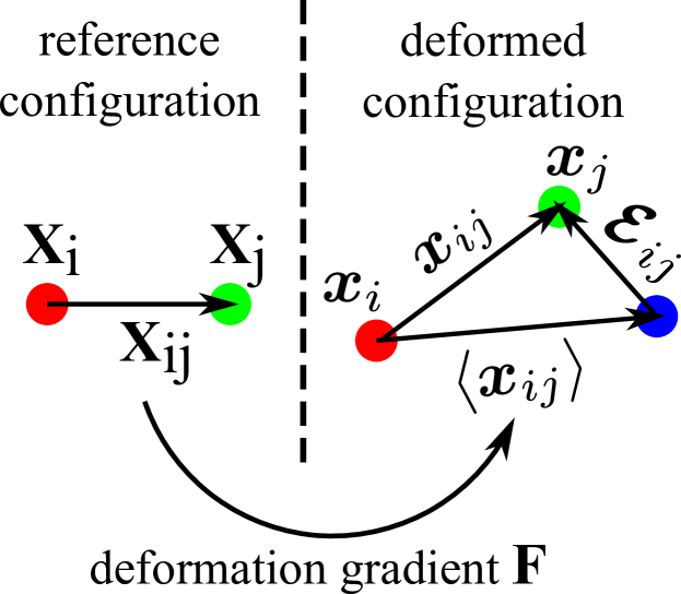
Figure 1: Illustration of the SPH stabilization scheme presented here. For any pair of particles $(i,j)$, the deformed image of the reference configuration distance vector $\left<\bm{x}_{ij}\right>=\bm{F}\bm{X}_{ij}$ is compared against the actual distance vector of the deformed coordinates, $\bm{x}_{ij}=\bm{x}_{j}-\bm{x}_{i}$. The difference between these vectors defines the error vector, $\bm{\mathcal{E}}_{ij}=\left<\bm{x}_{ij}\right>-\bm{x}_{ij}$, which is minimized by a penalty force.

To illustrate the idea of the SPH equivalent of an hourglass-control algorithm, consider the distance vector $\bm{X}_{ij}$ between a central node $i$ and a neighboring particle $j$ in the reference configuration. Applying the SPH approximation of the deformation gradient to this vector results in the approximated relative separation $\left<\bm{x}_{ij}\right>^{i}$,

$$\left<\bm{x}_{ij}\right>^{i}=\bm{F}_{i}\bm{X}_{ij}.$$ (25)

Note that the superscript $i$ denotes the application of $\bm{F}_{i}$ to $\bm{X}_{ij}$. Ideally, if the deformation gradient is exact, and there exists a unique mapping between all particles’ positions within the neighborhood of the central node and the deformation gradient, the approximated relative separation will coincide with the actual relative separation of the particles $i$ and $j$ in the deformed configuration. This situation is, however, typically not the case due the presence of integration errors. The difference of the approximated and actual relative separations defines the error vector,

$$\bm{\mathcal{E}}_{ij}^{i}=\left<{\bm{x}}_{ij}\right>^{i}-\bm{x}_{ij}.$$ (26)

Figure 1 gives a graphical representation of the error vector. To stabilize the system and suppress the hourglass modes, the magnitude of the error vector needs to be minimized. In this work, we formulate a correction force which is proportional to the magnitude of the error vector, i.e., we add stiffness to the system to counteract the hourglass modes. It is advantageous to formulate the correction force in terms of pairwise particle forces, as this approach conserves linear and angular momentum if the force is anti-symmetric with respect to interchange of the particle indices and co-linear with the particle separation vector. To this end, we measure that part of the error vector which points along the direction of the current particle separation vector:

$$\delta_{ij}^{i}=\frac{\bm{\mathcal{E}}_{ij}^{i}\cdot\bm{x}_{ij}}{x_{ij}}.$$ (27)

$\delta_{ij}^{i}$ is a scalar with dimensions of length that indicates the change of distance which the particle separation should attain in order to minimize the error vector. In what follows, a force that is linear in $\delta_{ij}^{i}$ is derived, and its stiffness is expressed using the Young’s modulus of the system.

Consider the potential energy density $\hat{\phi}$ (energy per unit volume) of a Hookean material subjected to uniaxial strain, i.e., a linear spring,

$$\hat{\phi}=\frac{1}{2}E\varepsilon^{2},$$ (28)

where $E$ is the Young’s modulus and $\varepsilon=(L-L_{0})/L_{0}$ is the uniaxial strain, with $L$ and $L_{0}$ being the current and rest length of the spring. The force density of this spring is

$$\hat{f}=-\frac{\mathrm{d}\hat{\phi}}{\mathrm{d}L}=-\frac{E}{L_{0}}\varepsilon.$$ (29)

In the context of the hourglass correction force, deviations of the length of the spring away from its rest length are due to a non-zero $\delta_{ij}^{i}$, and the rest length of the spring is the particle separation in the reference configuration. Thus, the hourglass correction force per unit volume between particles $i$ and $j$, and obtained using the deformation gradient of particle $i$ is:

$$\hat{\bm{f}}_{ij}^{i}=-\frac{E}{X_{ij}}\frac{\delta_{ij}^{i}}{X_{ij}}\frac{\bm{x}_{ij}}{x_{ij}}.$$ (30)

The above hourglass correction force can be improved in two aspects. (i) To be consistent with the SPH picture, where particle interactions are weighted according to volume and distance, a normalized smoothing kernel is introduced. (ii) The hourglass force is unsymmetrical with respect interchange of particle indices. Therefore, explicit symmetrization via the arithmetic mean is used. Thus, the expression for the smoothed and symmetrized correction force density between particles $i$ and $j$ reads:

$$\hat{\bm{f}}_{ij}^{HG}=-\frac{1}{2}\,\alpha\,W_{ij}\,\left[\hat{\bm{f}}_{ij}^{i}+\hat{\bm{f}}_{ji}^{j}\right],$$ (31)

where $\alpha$ is a dimensionless coefficient that controls the amplitude of hourglass correction, and $W_{ij}=W_{ij}\left(X_{ij}\right)$ is a smoothing kernel which depends on the distance in the reference configuration. Finally, the expression for the total hourglass correction force on particle $i$ due to all neighbors j is,

$$\bm{f}_{i}^{HG} = V_{i}\sum\limits_{j\in\mathcal{S}}V_{j}W_{ij}\hat{\bm{f}}_{ij}^{HG}$$ (32)

$$= \sum\limits_{j\in\mathcal{S}}-\frac{1}{2}\,\alpha\,\frac{V_{i}V_{j}W_{ij}}{X_{ij}^{2}}\,\left[E_{i}\delta_{ij}^{i}+E_{j}\delta_{ji}^{j}\right]\,\frac{\bm{x}_{ij}}{x_{ij}}.$$

This expression preserves both linear and angular momentum as the term within the sum is anti-symmetric and collinear with the particle separation vector.

3.2 Similarity to Laplacian stabilization

The above introduced SPH stabilization approach is derived using arguments which originate in hourglass control schemes for Lagrangian Finite Element Methods. It is noteworthy, however, that an analogy to a Laplacian stabilization scheme can also be derived, which is used with Eulerian Computational Fluid Dynamic (CFD) methods. The analogy will be derived for the one-dimensional case.

Following a classic paper by Jameson an Mavripilis [25], the flux of conserved quantities between adjacent cells is described by the following evolution equation,

$$\frac{\mathrm{d}}{\mathrm{d}t}S_{i}w_{i}=-Q(w_{i})+D(w_{i}).$$ (33)

Here, $i$ is the index of the cell, $S_{i}$ is the cell volume, $w_{i}$ is the vector of conserved variables, $Q(w_{i})$ is the flux of these variables, and $D(w_{i})$ denotes a stabilization term. This evolution equation bears some analogy to the equation of motion used in the Lagrangian SPH method, c.f. 24, if the force on a particle is used to define a momentum flux over a hypothetical interaction area. The cell-centered Euler CFD scheme allows decoupling between even and odd cells, which leads to zero-energy modes. The task of the stabilization term is therefore to add coupling by introducing higher-order terms, namely a second derivative of the conserved variables.:

$$D(w_{i})\propto\sum\limits_{n=1}^{NN}\nabla^{2}w_{i}.$$ (34)

The summation above includes all direct neighbors $NN$ of cell $i$. Specializing to one dimension only and using central differences, the second derivative is approximated by the undivided Laplacian $\tilde{\nabla}^{2}$,

$$\tilde{\nabla}^{2}w_{i}=w_{l,i}-2w_{i}+w_{r,i},$$ (35)

where only left and right neighbors with indices $l,i$ and $r,i$ of cell $i$ are considered. Thus, an explicit and computable expression for the stabilization term is obtained. The interpretation of this stabilization is that curvature of the solution field is suppressed, i.e., the solution is forced to be locally linear. The task at hand is now to show that the SPH hourglass control scheme proposed here can be equally expressed using an undivided Laplacian. To see this, we note from eqn. (32), that the hourglass correction force is proportional to the scalar hourglass error measure, which is a function of the deformation gradient:

$$f_{i}^{HG} \propto \sum\limits_{j\in\mathcal{S}}\delta_{ij}^{i}$$ (36)

$$\propto \sum\limits_{j\in\mathcal{S}}\frac{\left(\bm{F}_{i}\bm{X}_{ij}-\bm{x}_{ij}\right)\cdot\bm{x}_{ij}}{x_{ij}}$$ (37)

For the one-dimensional SPH case, only considering nearest neighbors as well as unit initial particle spacing and a constant SPH weight function, the deformation gradient is given by Bonet et al [13] as $F_{i}=(x_{r,i}-x_{l,i})/2$, Therefore, eqn. (37) is rewritten as

$$f_{i}^{HG} \propto \sum\limits_{n=1}^{NN}F_{i}X_{ij}-x_{ij}$$ (38)

$$\propto \sum\limits_{n=1}^{NN}\frac{x_{r,i}-x_{l,i}}{2}-(x_{r,i}-x_{i})$$ (39)

$$\propto \sum\limits_{n=1}^{NN}-\left(x_{l,i}-2x_{i}+x_{r,i}\right)$$ (40)

$$\propto \sum\limits_{n=1}^{NN}-\tilde{\nabla}^{2}x_{i}.$$ (41)

Note that in eqn. (39), the arbitrary substitution $x_{ij}=x_{r,i}-x_{i}$ has been made. This analysis shows that the here presented hourglass correction scheme can be expressed using the undivided Laplacian of the coordinate field. Therefore, the same interpretation of the stabilization as in the CFD case holds: curvature in is penalized, such that the deformation field is forced to be locally linear. This interpretation is in agreement with motivation of the SPH hourglass control scheme, namely that the deformation gradient, which is a linear operator, should be able to accurately describe the deformation field.

4 Validation examples

In the following, a number of test cases is presented which demonstrate the correctness and the advantages of the hourglass correction scheme presented here. All test cases are computed using 2d plane-strain conditions and Desbrun’s Spiky Kernel [26] is used. It is emphasized that no artificial viscosity or other dissipative mechanisms are employed to stabilize the simulations reported here.

4.1 Patch test and stability

The patch test can be regarded as the most basic test for a solid mechanics simulation code. A strip of some material that is discretized using several elements (or SPH particles) is subjected to a uniform strain field and the stress is computed. Regardless of the discretization, the stress should be uniform everywhere. SPH with first-order corrected kernel gradients is well-known to pass this test. Here, however, we are interested in the subsequent time-integration following such an initial perturbation. To this end, a random initial particle configuration is obtained by discretizing a square patch of edge length 1 m and uniform area mass density $\rho=1\mathrm{kg/m^{2}}$ into 444 quadliteral area elements using a stochastic algorithm based on triangular Voronoi tesselation and recombination of the triangles into quadliterals. Particle volumes and masses are obtained from the quadliteral area and the prescribed mass density. The SPH smoothing kernel radius is adjusted individually for each particle such that approximately 12 neighbors are within the kernel range. Such a non-uniform particle configuration poses extreme stability challenges to normal SPH. Figure 2 shows the initial particle configuration. The material model is chosen as linear elastic with $E=1\>\mathrm{Pa}$ and $\nu=0.3$. The patch is uniformly stretched by 10% along both axes. After this initial perturbation, the system is integrated in time using a standard leap-frog algorithm with a CFL-stable timestep, resulting in a periodic contraction and expansion mode. Figure 3 compares SPH with and without hourglass stabilization. In the unstabilized system, particle motion is not coherent and particle disorder is observed already after the first contraction. After eight contractions, particle disorder is very pronounced and the motion of the patch is entirely dominated by numerical artifacts. A stabilized simulation was conducted with an hourglass control coefficient $\alpha=50$. This particular value was found to mark the threshold where a clear improvement in stability can be observed. This stabilized simulation exhibits a completely coherent particle motion, and can be continued for hundreds of oscillations. It is noted that the stabilization increases the apparent stiffness of the system – in this case by roughly 3% as computed from the oscillation frequency. This effect is similar to hourglass control mechanisms in Finite Element methods, where care has to be taken as to much hour-glassing control is applied in order to preserve the desired material behavior. This example is concluded by noting that the here presented hourglass stabilization mechanism leads to a dramatic increase of the simulation stability even with difficult particle configurations. A video showing the stabilized and unstabilized simulations is provided as online supplemental data for this article.

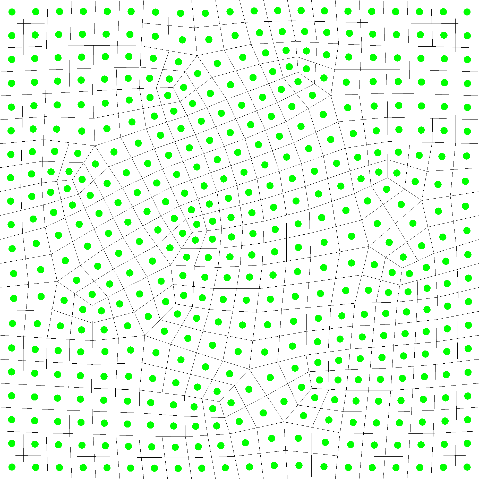
Figure 2: Initial particle arrangement for the patch test stability example. A random initial particle configuration is obtained by discretizing a square patch into 444 quadliteral area elements using a stochastic algorithm based on triangular Voronoi tesselation and recombination of the triangles into quadliterals. The particle coordinates are taken to be the quadliteral element centers and particle volumes are taken as the quadliteral area times a unit thickness.

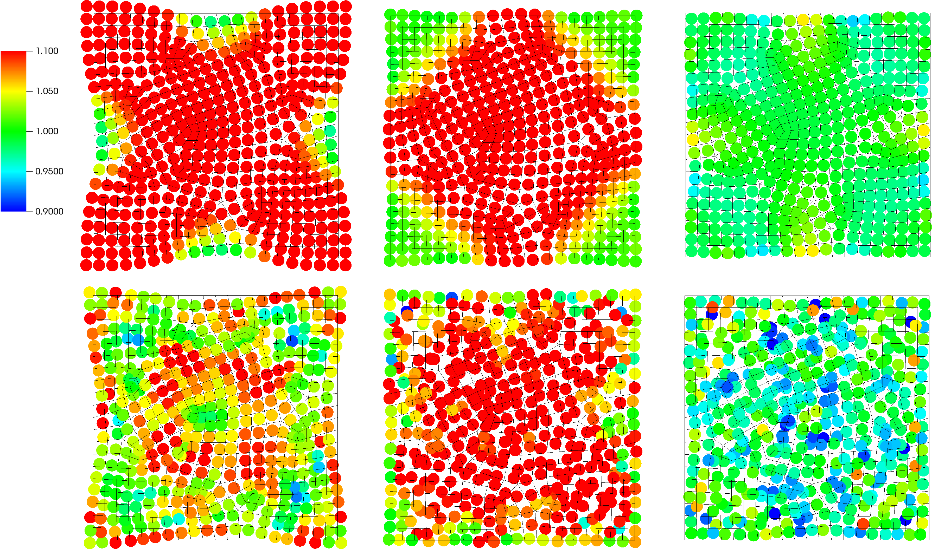
Figure 3: Simulation snapshots comparing unstabilized and stabilized trajectories. A 2d patch of an elastic material is perturbed by isotropic stretch of 10 % and integrated in time, resulting in a periodic contraction and expansion mode. The top row of images shows the simulation stabilized with an hourglass control coefficient $\alpha=50$ during the first, third, and tenth contraction period. The bottom row shows corresponding snapshots from an unstabilized simulation. The mesh in the background serves as a guide to the eye.

4.2 Bending of a beam

This example tests the accuracy of the stabilized SPH scheme against the analytic Timoshenko solution to the bending of a simply supported beam with dimensions $8\,\mathrm{mm}\times 1\,\mathrm{mm}$, see Fig. 4.The material model of the beam is taken as linear elastic with Youngs modulus $E=100\,\mathrm{GPa}$ and $\nu=0.3$. As this is a 2d plane strain problem, the effective 2d Youngs modulus is

$$E_{2d}=\frac{E}{1-\nu^{2}}\simeq 109.89\,\mathrm{GPa}$$ (42)

Timoshenko’s solution [27] for this problem results in a compliance (the ratio of applied displacement to the resulting force) $C_{theory}=f/u\simeq 0.053657\,\mathrm{kN}/\mathrm{mm}$. For the numerical SPH solution, the beam is discretized using a 2d square lattice with a total number of particles $N=n_{x}\times n_{y}=(3+8n)\times n$, with $n\in\left[4,8,16\right]$. The smoothing kernel radius is chosen as 2.41 times the lattice spacing, such that the number of neighbors is constant for all discretizations. The beam is clamped at the left end by enforcing zero displacements for the three leftmost columns of particles. A downwards displacement boundary condition of maximum amplitude $u_{y}=0.1\,\mathrm{mm}$ is applied at the top right particle with a velocity of 0.1 mm/s which corresponds to quasi-static loading. The reaction force $f$ is measured at this particle, resulting in the numerical compliance $C_{num}$. To quantify the accuracy of the numerical solution, the $L^{2}$-norm of the relative error between the numerical solution and the analytic solution is defined as

$$\mathrm{error}=\sqrt{\left(\frac{C_{num}-C_{theory}}{C_{theory}}\right)^{2}}.$$ (43)

Fig. 5 reports error values for an unstabilized simulation and a stabilized simulation for different discretization length scales. For the unstabilized simulation, the convergence rate is approximately -1.45. It is not clear how to understand this odd rate of convergence, as the Lagrangian SPH method employed here uses a kernel gradient approximation which is correct to first order. Therefore, all linear terms in the solution should be computed exactly such that only terms of second order terms contribute to the error, and one might speculate that integration errors due to nonlinear modes increase the errors. In contrast to this behavior, we observe that the stabilized simulation yields almost exactly quadratic convergence as well as much lower relative error values. This result is remarkable, as – to the best of this author’s knowledge – no other nodal integration scheme is able to yield quadratic convergence, and only computationally expensive cell integration methods have been reported to perform in this manner [15]. A parameter study of the hourglass control coefficient reveals that the factor $\alpha=50$, which was observed to mark the threshold beyond which the patch test simulation from the previous section was clearly stabilized, is also a good choice for the beam bending problem. As can inferred from Table 1, which lists the convergence rates and the relative errors of the simulation with the finest discretization for different values of $\alpha$ are listed, the convergence rate and error magnitude is nearly optimal for $\alpha=50$. The author is aware that other optimal values might be determined for different simulation problems, however, for the limited scope of this work, $\alpha=50$ is used henceforth for all stabilized simulations.

Table 1: Parameter study for the hour-glassing control coefficient $\alpha$ and the bending problem of a simply supported beam. The rate of convergence refers to the power law exponent which describes how the numerical solution approaches the analytic solution upon discretization refinement. The relative error quotes the magnitude of deviation between the finest discretization and the analytic solution.

$\alpha$	convergence rate	error at finest discretization
0	-1.45	$24.5\times 10^{-4}$
25	-1.65	$18.7\times 10^{-4}$
50	-1.97	$6.6\times 10^{-4}$
75	-1.78	$21.9\times 10^{-4}$
100	-1.74	$31.7\times 10^{-4}$

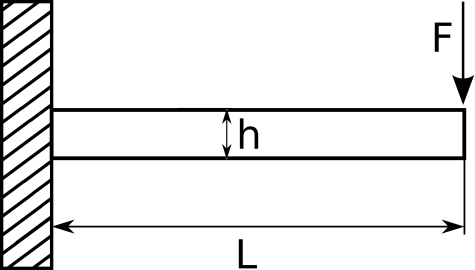
Figure 4: Sketch of the simply supported beam with dimensions $L=8\,\mathrm{mm}$ and $h=1\,\mathrm{mm}$.

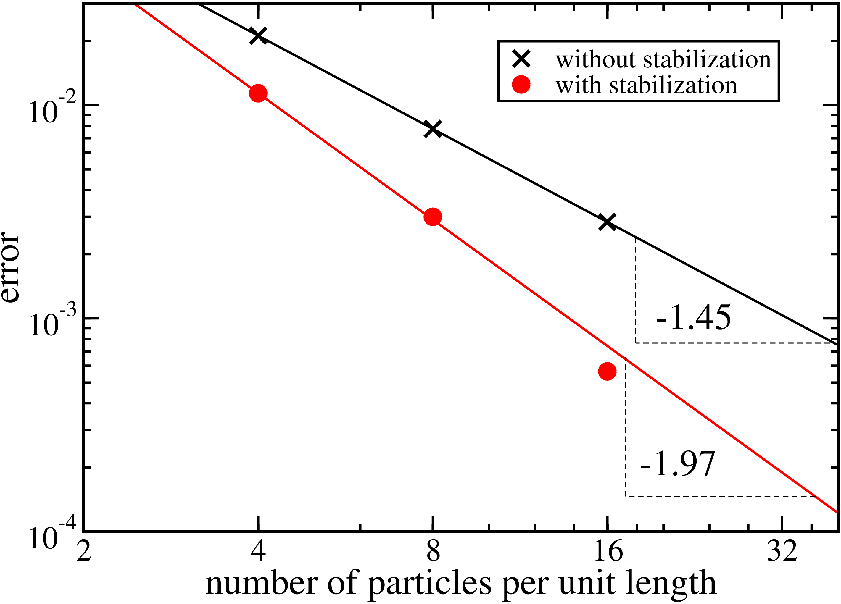
Figure 5: Relative errors of the SPH solution to the bending problem for the simply supported beam. The unstabilized solution employs hourglass control with $\alpha=50$, while the unstabilized solution uses $\alpha=0$.

The above test case has only considered a maximum beam deflection which is small compared to the beam dimensions for the purpose of comparing against an analytic solution. It is instructive to extend this example to very large deflections. To this end, a large boundary displacement $u_{y}=8\,\mathrm{mm}$ is applied, and stabilized and unstabilized simulation results are qualitatively compared. Snapshots of the simulations corresponding to the same boundary displacements, are shown in Fig. 6. In the first snapshot at $u_{y}=4.8\,\mathrm{mm}$, no obvious difference between both simulations can be observed. For the second snapshot at $u_{y}=6.6\,\mathrm{mm}$, the unstabilized simulation shows a pattern where pairs of particles in the interior of the beam move together and do not follow the rotation of the beam’s neutral line. Clearly, the unstabilized system tries to minimize its elastic energy by assuming a configuration which is not in agreement with a linear displacement field. This leads to an obviously wrong particle configuration for the last snapshot at $u_{y}=8.0\,\mathrm{mm}$. In contrast, the stabilized system with $\alpha=50$ shows particle displacements which appear very reasonable and exhibit no instability.

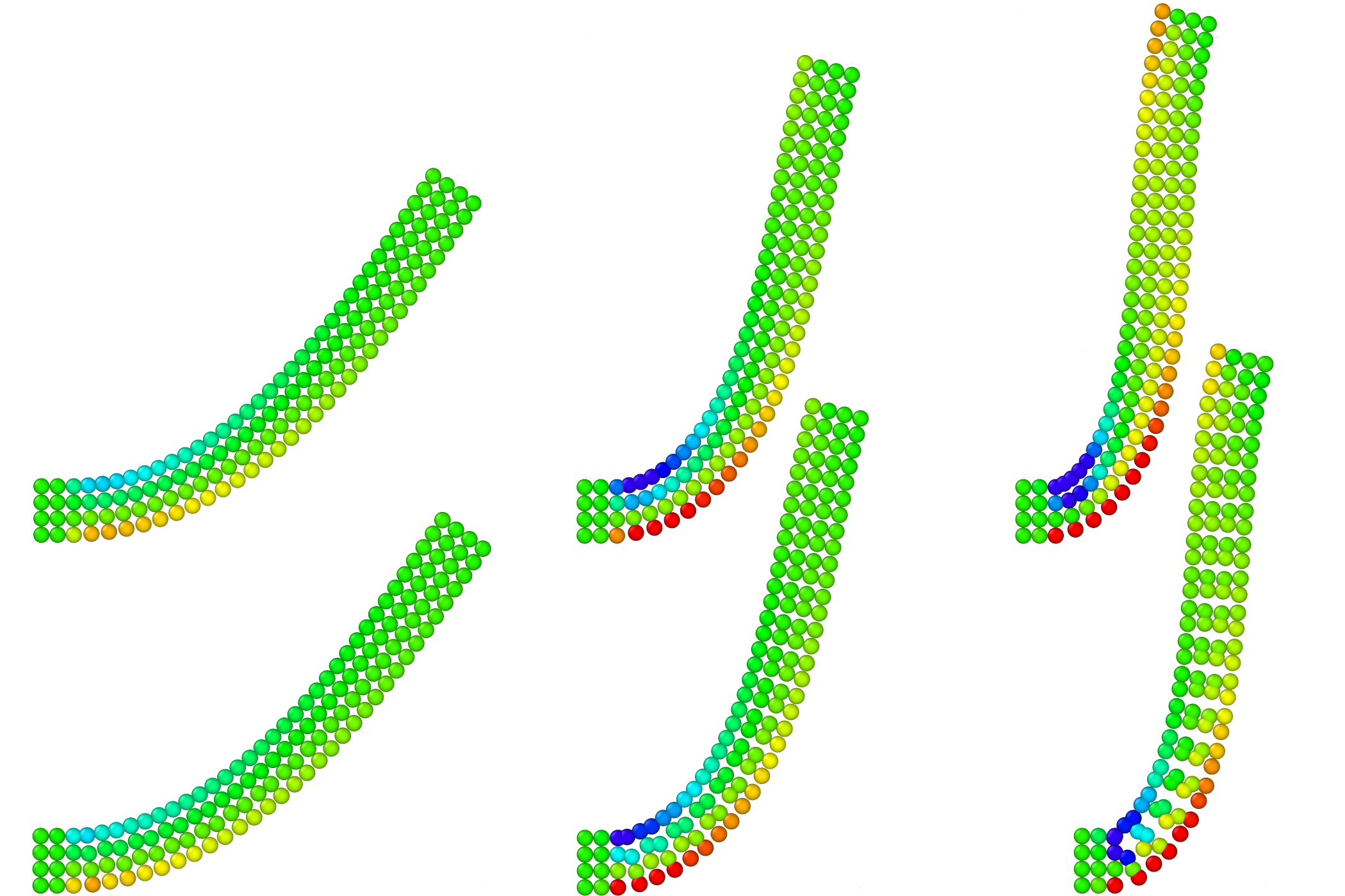
Figure 6: Comparison of stabilized (top) and unstabilized results for a large deflection simulation of the simply supported beam. The color coding represents the $xx$-component of the Second Piola-Kirchhoff stress tensor, with red signifying tension and blue compression.

We conclude this test case by noting that Total-Lagrangian SPH can become unstable for certain loading conditions even with perfectly uniform reference particle configurations. The here proposed hourglass-control algorithm removes these instabilities and increases accuracy as well as convergence rate.

4.3 Punch Test

The punch test is a classic example for a difficult large deformation test. It was first applied to a meshless method in order to demonstrate the stability of the Reproducing Kernel Particle Method, which combines kernel approximation techniques with Gaussian integration on a background mesh [28]. In the punch test, a block of a rubber-like material is compressed by a rigid rectangular tool with sharp edges. As the compression proceeds, the material moves outwards to open sides. The punch tool digs into the material and causes large stress concentrations at its sharp corners. This problem is difficult to simulate with FEM and impossible with unstabilized Lagrangian SPH [29]. The rubber material is described by a compressible Neo-Hookean model [22],

$$\bm{S}=\mu\left(\bm{I}-\bm{C}^{-1}\right)+\lambda(\ln J)\bm{C}^{-1},$$ (44)

where $\lambda=E\nu/[(1+\nu)(1--2\nu)]$ and $\mu=E/[2(1+\nu)]$ are the Lamé constants, $J$ is the determinant for the deformation gradient $\bm{F}$, and $\bm{C}=\bm{F}^{T}\bm{F}$. The rubber is given by a rectangular block of dimensions $6\,\mathrm{mm}\times 3\,\mathrm{mm}$, which is discretized using a square lattice with lattice constant $l_{0}=1/15\mathrm{mm}$. The material parameters Young’s modulus and Poisson ratio are taken as $1\,\mathrm{GPa}$ and 0.45, respectively. The compression tools are modelled as thin blocks of a rigid material with dimensions $6\,\mathrm{mm}\times 0.15\,\mathrm{mm}$, discretized as a square lattice of particles with lattice constant $l_{1}=l_{0}/4$. The tool particles interact with the rubber particles via a repulsive Hertzian potential [30] which utilizes the same Young’s modulus as the rubber and is effectively so stiff that no mutual penetration can occur.

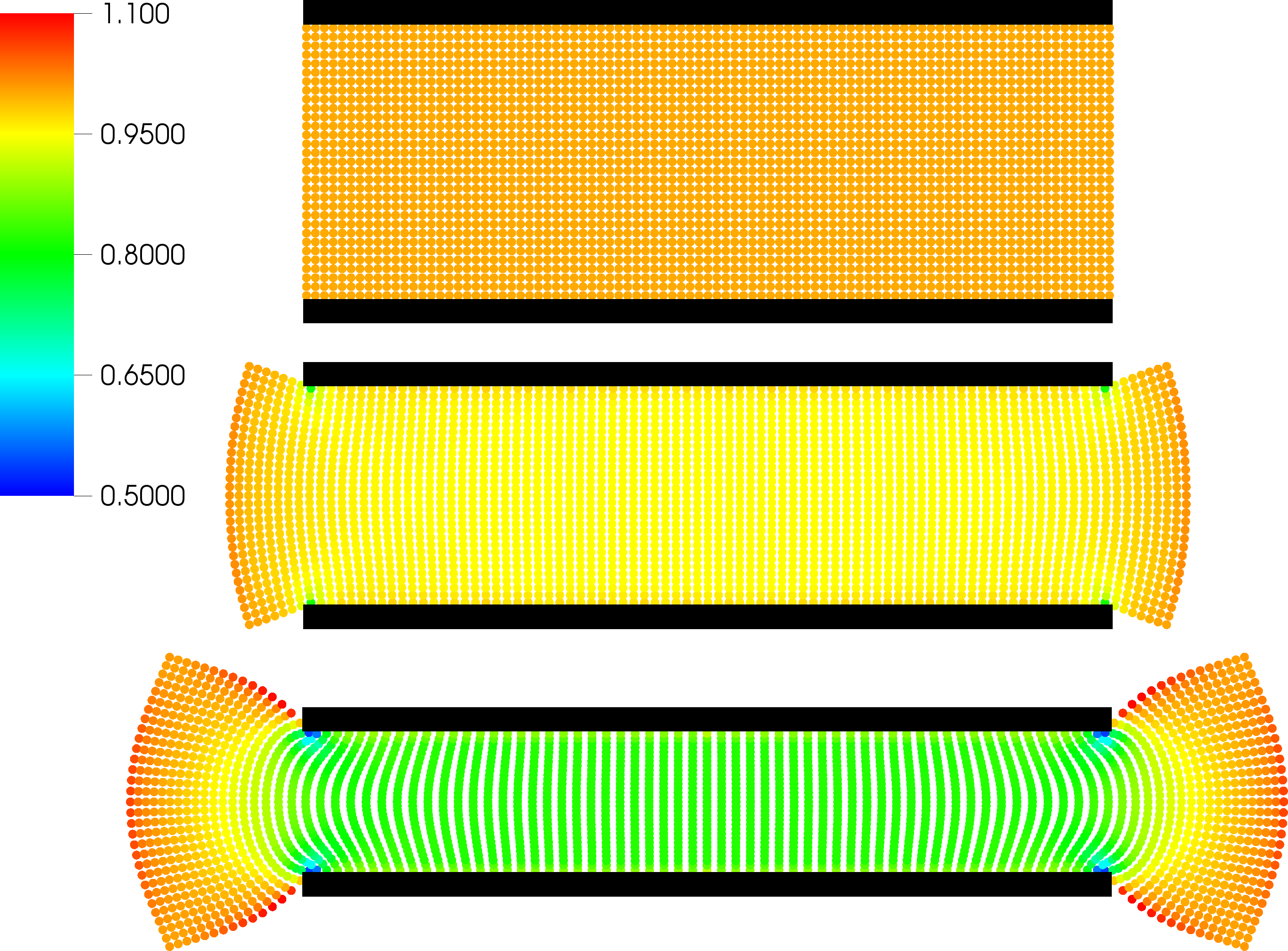
Figure 7: Snapshots of the punch test simulation corresponding to vertical compression states of 0%, 10% and 50%. Rubber particles are colored according to the determinant of the deformation gradient. Note the strong gradient of volumetric strain at the corners of the compression tool plates, which are shown in black.

The simulation is performed with a compression velocity of 1 mm/s, which can be considered quasi-static, and a stabilization parameter $\alpha=50$. Simulation snapshots are shown in Fig. 7. The simulation,proceeds without any sign of instabilities until a vertical compression ratio of 50% is reached. Higher velocities up to 100 mm/s and further compression up to 90% were also simulated, however, strongly dynamic compression rates necessitate the use of artificial viscosity to keep the simulation stable. This test case is concluded by noting that an otherwise difficult simulation problem can be easily handled using Total-Lagrangian SPH stabilized with the hourglass control mechanism presented here.

4.4 Rubber Pull Test

In this example, a strip of rubber is subjected to a 500% increase in length. This test case is also taken from [28], where it serves as a very large deformation test to demonstrate the stability of the RKPM method. The rubber strip is initially quadratic with dimensions of $2\,\mathrm{mm}\times 2\,\mathrm{mm}$ and discretized using a square lattice with lattice constant $l_{0}=1/15\,\mathrm{mm}$. The smoothing kernel radius is taken as $2l_{0}$. The top and bottom row of particles are subjected to a velocity boundary condition $\bm{v}=(0,\pm 0.1\mathrm{mm/s})$ which causes quasi-static elongation of the rubber strip, while no lateral displacement is possible for these rows of particles. This setup corresponds to the clamping condition typically encountered in material test stands. The same compressible Neo-Hookean material model is used as in the previous test case. The simulation is carried out until the length of the rubber strip has increased to $12\,\mathrm{mm}$. Fig. 8 compares the final state of an unstabilized simulation with that of a simulation stabilized with $\alpha=50$. The unstabilized simulation exhibits particle disorder, in particular near the boundaries of the domain. A pairing of rows of particles, alternating with larger gaps, similar to the pairing effect seen in the large deflection simulation of the simply supported beam, can be observed. No such instabilities are present in the stabilized simulation, which features a very smooth deformation field.

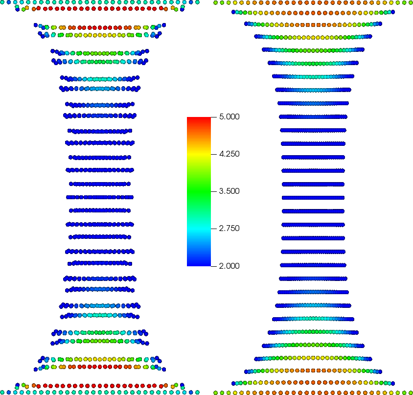
Figure 8: Comparison of unstabilized (left) and stabilized (right) simulation snapshots for the rubber strip pull test case. An initially quadratic rubber strip is elongated in the vertical direction until a strain of 500% is reached. The snapshots are scaled here in the vertical direction to better fit them on the page. Color coding of the particles represents the determinant of the deformation gradient.

4.5 Taylor impact

All of the preceding test cases have investigated elastic material behavior only, without any kind of material instability. The deformation field for an elastic material is typically very smooth, in contrast to a plastic deformation, which is governed by the localization of deviatoric stress. This localization is usually well defined with a sharp boundary, e.g., in the case of adiabatic shear bands. To successfully cope with plastic deformations, the numerical solution scheme must therefore allow some desired nonlinearities to develop, while other nonlinearities, e.g. zero-energy modes, must be suppressed. This requirements poses a severe challenge to the hourglass-control algorithm presented here. Let us briefly remind ourselves what the effect of this algorithm is: the deformation associated with a line element in the current configuration is compared against the result of using the deformation gradient (which is a linear operator) on a line element in the reference configuration. Deviations between both deformations are minimized by a penalty force. This means that the deformation field is forced to be locally (on the scale of the smoothing kernel radius) linear. It is therefore expected that localization phenomena such as plastic deformation are suppressed by the hourglass control mechanism. This behavior is again similar to what is observed for hourglass control schemes in FEM: there, the amplitude of the control force has to be scaled down by orders of magnitude in order to permit plastic deformation, or indeed fluid flow, to happen.

With this in mind, the SPH hourglass control mechanism is reformulated as follows. All SPH particles with a zero value of plastic deformation utilize the expression already given by eqn. (32). For any SPH particle with a non-zero value of plastic deformation, the Young’s modulus in eqn. (32) is replaced by the yield strength, which is typically much smaller than the Young’s modulus.

As a plastic deformation test case, the impact of an aluminum bar against a rigid plate is considered. The material parameters are given by Young’s modulus $E=\mathrm{78.2\ GPa}$, yield strength $\sigma_{Y}=1.0\mathrm{\ GPa}$, Poisson ratio $\nu=0.3$, and mass density $\rho=\mathrm{2700\ kg\,m^{-3}}$. The aluminum bar travels at an initial velocity of $v_{0}=\mathrm{373\ m\,s^{-1}}$ and has dimensions of $3.91\,\mathrm{mm}\times 23.46\,\mathrm{mm}$. It is discretized using a square lattice of particles with a lattice spacing of $l_{0}=0.35\,\mathrm{mm}$. The smoothing kernel radius is taken as $3l_{0}$. The material model used here is linear elastic – perfectly plastic and based on the multiplicative decomposition of the total deformation gradient in elastic and plastic parts, which is described in detail in Appendix A of [22].

The simulation is carried out until the development of plastic deformation is complete. Fig. 9 compares the unstabilized solution against the stabilized solution. The general shape of the deformation appears reasonable, and is similar to published results for the 2d axissymetric case [28], even though the 2d plane-strain case is considered here. The unstabilized simulation exhibits particle disorder, which is particularly pronounced in the regions of strong plastic deformation, but also extends into regions with only elastic deformation. We note that the addition of a reasonably small amount of artificial viscosity would prevent the occurrence of particle disorder. For the purpose of demonstrating the onset of instability, however, we chose to report results with no artificial viscosity. It is likely, that all SPH results published for this and similar problems use dissipative mechanisms to keep the solution smooth. In the case of the stabilized simulation, a smooth deformation field is obtained without the need for artificial viscosity. The overall shape of the deformed aluminum bar is similar to the unstabilized solution, indicating that plastic flow was not excessively suppressed by the stabilization algorithm. It is noted, however, that if no reduction of the hourglass control amplitude as discussed above is performed, plastic deformation does not occur and the aluminum bar rebounds elastically from the rigid surface.

This example is concluded by noting that the SPH hourglass control algorithm presented here may be used to simulate material instabilities such as plastic deformation, but care has to be taken as to how much hour-glassing control is applied.

Figure 9: 2d Taylor impact test. The material model is linear-elastic / ideal plastic. Color coding is the norm of the plastic strain tensor. The left image shows the unstabilized SPH solution with clearly visible particle disorder. In contrast, SPH stabilized with the here proposed algorithm results in a smooth solution.

4.6 Tensile test of a 3d specimen with failure

The purpose of this test example is to compare the failure behavior of SPH with the here presented stabilization algorithm against unstabilized SPH and a FEM solution (reduced integration elements with one Gauss point). A 3d tensile test specimen is elongated at $10\,\mathrm{mm}/\mathrm{ms}$ until failure occurs. The material model used is linear-elastic with $E=\mathrm{10\ GPa}$, $\nu=0.3$, and $\rho=\mathrm{2700\ kg\,m^{-3}}$. For SPH, failure is realized with a damage rate model similar to [31], which accumulates damage if any current principal strain value exceeds a pre-defined value $\epsilon_{max}=0.08$:

$$\frac{\mathrm{d}D^{1/3}}{\mathrm{d}t}=0.4\,\frac{c_{0}}{h}$$ (45)

In the equation above, $0.4\,c_{0}$ is the damage propagation speed which ensures that a crack does not propagate faster than the speed of sound $c_{0}$ over a characteristic distance $h$, here taken as the SPH kernel radius. The scalar damage variable is used to scale the components $\sigma_{i}$ of the principal (diagonalized) stress tensor only if the component is positive, i.e., damage is only allowed for tension and not for compression:

$$\tilde{\sigma}_{i}=(1-D)\,\sigma_{i}$$ (46)

The scaled stress tensor $\tilde{\sigma}$ is then used to compute interparticle forces. In the case of FEM, failure is realized by instantaneously eroding those elements which exceed the maximum principal strain. Fig. 10 compares snapshots of stabilized and unstabilized SPH solutions with the FEM solution. The comparison indicates that stress distribution of the stabilized SPH solution is as smooth as the FEM solution and concentrates at the center of the test specimen, where the minimum cross section is located. In contrast, the stress distribution of the unstabilized SPH solution is affected by the non-uniform particle spacing and exhibits alternating stripes of low and high stress values. As a result, failure is incorrectly predicted at an off-center position. The stabilized SPH solution, however, correctly predicts failure at the center, in agreemeent with FEM.

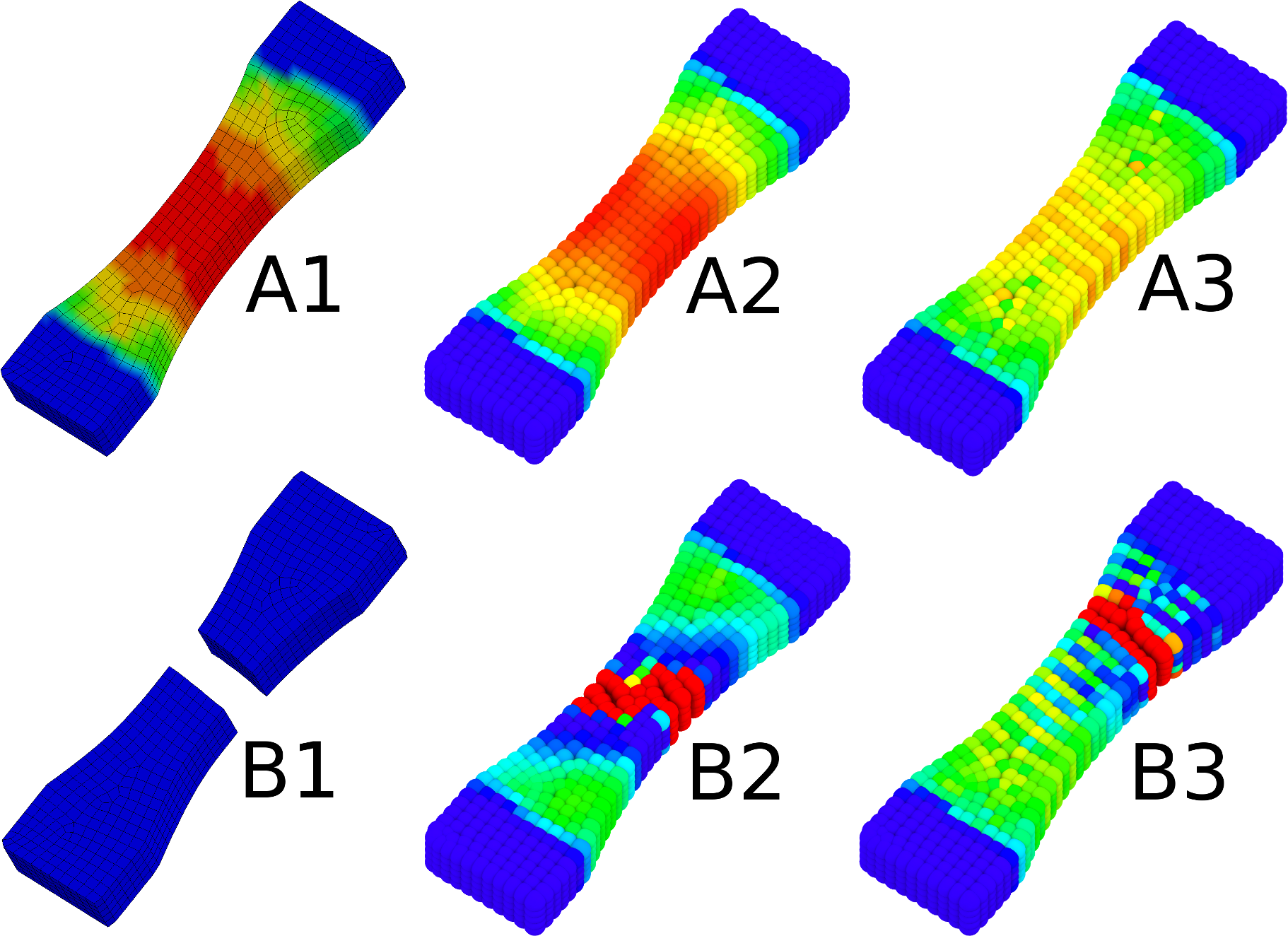
Figure 10: Comparison of stabilized and unstabilized SPH with FEM. The test specimen with a gauge cross section of $15\times 10\,\mathrm{mm}$ is discretized for FEM using 1800 solid elements. The SPH mesh is derived by placing a particle at the barycenter of each element, and choosing the kernel radius such that 30 neighbors are obtained. Images A1 and B1 show the FEM solution just before and after failure. A2/B2 show the same snapshots for the stabilized SPH simulation, while A3/B3 show the unstabilized SPH simulation. The color coding respresents maximum principal strain, increasing from blue to red

It is also of interest to quantitatively compare the reaction force at the clamped ends of the tensile specimen for the three different simulation approaches. Fig. 11 shows that stiffness obtained with SPH agrees very well with the FEM solution. However, the unstabilized SPH solution predicts failure at a displacement value which is 15% smaller than the FEM solution. In case of the stabilized SPH solution, this value decrease to 4%. The comparison therefore suggests that Total Lagrangian SPH stabilized with the here presented algorithm yields a similar accuracy as FEM with reduced integration elements, if the discretization is maintained at a similar level, i.e., elements are replaced with particles on a one-to-one basis.

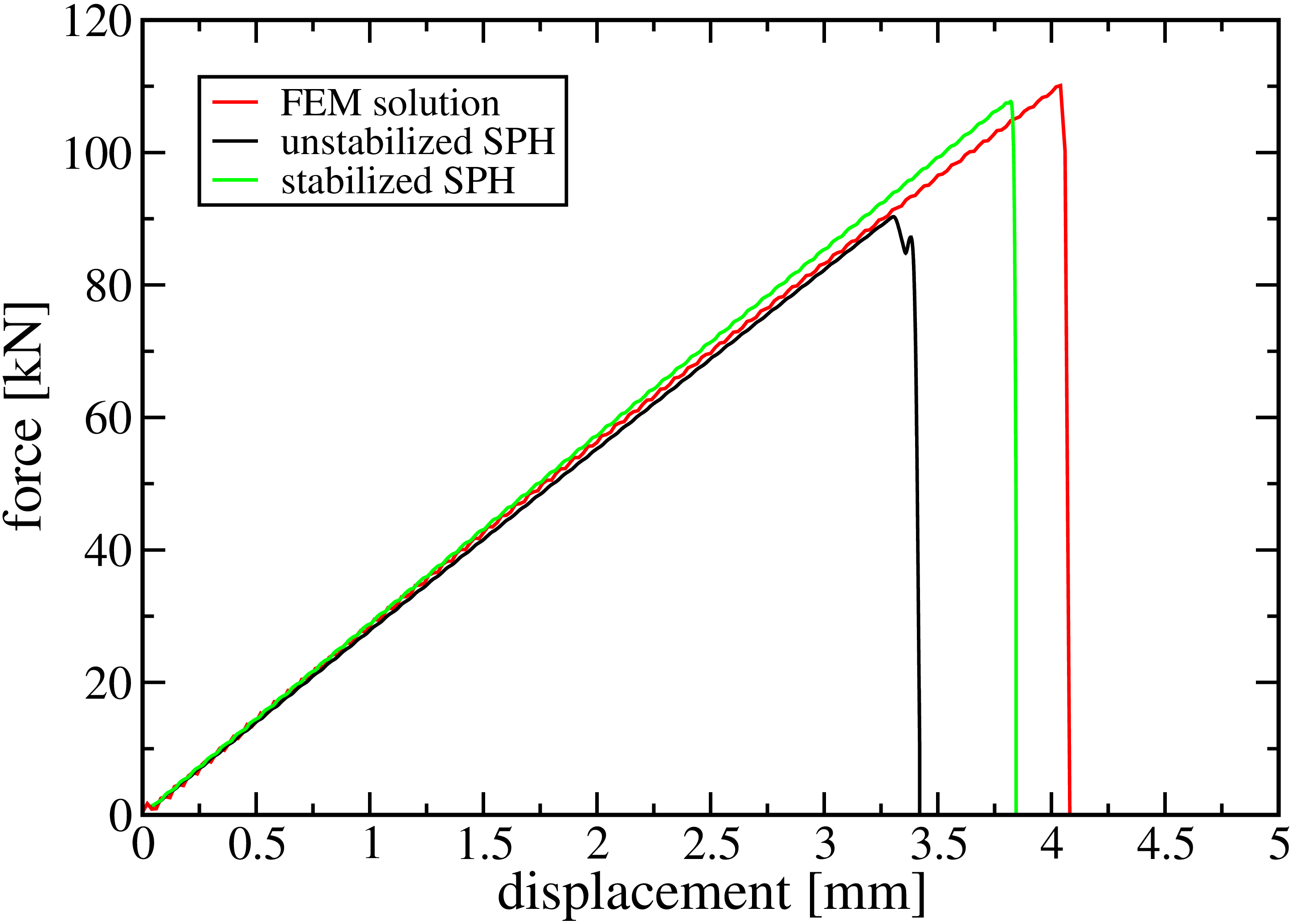
Figure 11: Force/displacement data for the 3d tensile test. Comparison is made between stabilized and unstabilized SPH, and a FEM reference solution.

5 Discussion

This paper presents a stabilization scheme for Smooth-Particle Hydrodynamics (SPH). The Total-Lagrangian formulation of SPH is considered, which does not suffer from tensile instability [6], but is still affected by another instability caused solely by the collocation character: rank-deficiency [7]. The mathematical meaning of rank-deficiency is that the solution to the underlying equilibrium equations which are discretized with SPH is non-unique. A physical interpretation of this non-uniqueness is obtained by considering particle positions and the deformation field. Within the kernel radius of a particle, there can be a manifold of different arrangements of particles which all result in the same SPH approximation of the deformation gradient. The deformation gradient results in a strain measure, which, via the material model, results in a stress state with an associated elastic energy. Oscillatory modes between the non-unique arrangements of particles cannot be suppressed, because the states which are linked by the oscillations are not distinct in terms of elastic energy. Thus, these oscillations modes can be populated with arbitrarily high amounts of kinetic energy until the solution is entirely dominated by this artifact, such that the simulation can be essentially considered as failed.

Various methods have been proposed to suppress these modes. Of particular importance are the addition of stress points [7, 10], which eliminate the rank-deficiency at the cost of an additional integration overhead. While this approach is very clean and attractive from a mathematical perspective, it appears somewhat impractical to use and not many researchers have taken up this approach, as judging from the available literature. An alternative approach is to suppress the growth of the instability modes by simply damping them out. This can be conveniently realized via the use of artificial viscosity , or conservative smoothing [9, 8]. However, by doing so, the simulation typically becomes more dissipative or dispersive in nature as one would like it to be.

This article introduces a completely different and new method to suppress the instability modes. The method is inspired by stabilization algorithms used in a non-particle method, namely the Finite-Element Method (FEM), which exhibits a very similar instability if rank-deficient elements are employed. In FEM, this instability is termed hour-glassing, and it is counteracted by suppressing non-linear deformation modes [18]. This work adapts this approach by identifying suppressing all modes which are not described by the deformation gradient. As the deformation gradient is a linear operator, a linear deformation field is enforced, and, at the same time, a unique correspondence between pairs of particle displacements and the deformation gradient is established.

The performance of the resulting stabilization algorithm is assessed using a number of linear elastic and elastoplastic test cases. In the case of the bending of a beam, a very desirable result is obtained: For a certain range of the amplitude of the stabilization force, quadratic error convergence is observed. This result is remarkable as it indicates that the stabilized numerical solution treats all linear terms correctly, such that remaining errors are solely of second order. This is precisely what one would expect from a numerical scheme which is first-order correct, such as gradient-corrected SPH. However, results reported for unstabilized SPH show convergence behavior which is less than quadratic [15], presumably because numerical artifacts affect the solution. Thus, the stabilization scheme reported here provides a clear improvement.

In the case of large rotation and deformations, much improved stability behavior is observed when compared to unstabilized SPH. The stabilized solution is always smooth, even in the case of the difficult punch test. In contrast, unstabilized SPH exhibits instabilities which are typically characterized by pairwise clumping of particles. Improved stability is also obtained for plastic deformations, however, the amplitude of the stabilization algorithm must be carefully chosen in this case, as too much stabilization inhibits plastic flow. This behavior is very similar to hour-glassing control mechanisms in FEM, where the amount of hour-glassing control typically has to be scaled down by orders of magnitude for plasticity problems when compared to purely elastic deformations [32]. This behavior is not ideal, but the here presented conditional switch, which reduces the stabilization strength at the onset of plastic deformation, appears to work to a satisfactory degree. Future work along these lines should address a viscous – rather than stiffness – based formulation of the stabilization algorithm.

It is noteworthy to discuss another stabilization algorithm for Total-Lagrangian SPH. Vidal et al. developed an approach, which minimizes a local measure of the Laplacian of the deformation field. Their approach results in much enhanced stability, such that updates of the reference configuration can be performed, yielding a stabilized updated Lagrangian scheme. Their work is seminal in the sense, that (i) updates of the reference configuration were identified to be a cause for the occurence of zero-energy modes, and (ii) higher-order derivatives could be used to suppress such instabilities. However, the algorithm involves the computation of a third-order tensor, which – in this author’s experience – dramatically affects the numerical efficacy. Additionally, the stabilizing effect is not very clear for large deformations, as the authors report that the punch test (c.f. Sec. 4.3) cannot be performed without updates of the reference configuration. In contrast, the stabilization scheme reported here, which is based on the deformation gradient bears negligible impact on the speed of the simulation. Early results of applying the new stabilization scheme to the updated Lagrangian formalism indicates that it also works very well, however, these results are outside the scope of the current article and will be published elsewhere.

What are the implications of this work? The stabilization algorithm reported here dramatically extends the range of deformations that can be simulated with Total-Lagrangian SPH in a stable and manner, without resorting to highly dissipative mechanisms. The new method is not affected by non-uniform particle configurations, as shown by the patch test. As the deformation field remains smooth, even for large deformations, numerical artifacts are less of an issue compared to standard SPH, such that higher accuracy is obtained. This statement is supported by the enhanced error convergence rate observed in the beam bending problem. Because the new stabilization algorithm bears analogies to hour-glassing control for FEM, the effect of the additionally introduced stiffness can be understood and judged using the large body of literature published for that method. The current method is straightforward to implement, and does not incur any significant computational overhead. It is therefore expected that this contribution pushes SPH away yet another step away from its academic status towards a method that can actually be used in practice for the reliable simulation of large deformation problems.

References

- [1] L. B. Lucy, A numerical approach to the testing of the fission hypothesis, The Astronomical Journal 82 (1977) 1013–1024.
- [2] R. A. Gingold, J. J. Monaghan, moothed particle hydrodynamics: theory and application to non-spherical stars, Mon. Not. Royal. Astr. Soc. 181 (1977) 375–389.
- [3] V. Springel, Smoothed particle hydrodynamics in astrophysics, Annual Review of Astronomy and Astrophysics 48 (1) (2010) 391–430. doi:10.1146/annurev-astro-081309-130914.
- [4] M. Gomez-Gesteira, B. D. Rogers, R. A. Dalrymple, A. J. Crespo, State-of-the-art of classical sph for free-surface flows, Journal of Hydraulic Research 48 (2010) 6–27. doi:10.1080/00221686.2010.9641242.
- [5] L. D. Libersky, A. G. Petschek, Smooth particle hydrodynamics with strength of materials, in: H. E. Trease, M. F. Fritts, W. P. Crowley (Eds.), Advances in the Free-Lagrange Method Including Contributions on Adaptive Gridding and the Smooth Particle Hydrodynamics Method, Vol. 395 of Lecture Notes in Physics, Berlin Springer Verlag, 1991, pp. 248–257. doi:10.1007/3-540-54960-9_58.
- [6] J. W. Swegle, D. L. Hicks, S. W. Attaway, Smoothed particle hydrodynamics stability analysis, Journal of Computational Physics 116 (1) (1995) 123–134.
- [7] C. T. Dyka, P. W. Randles, R. P. Ingle, Stress points for tension instability in sph, International Journal for Numerical Methods in Engineering 40 (1997) 2325–2341. doi:10.1002/(SICI)1097-0207(19970715)40:13<2325::AID-NME161>3.0.CO;2-8.
- [8] D. L. Hicks, J. W. Swegle, S. W. Attaway, Conservative smoothing stabilizes discrete-numerical instabilities in SPH material dynamics computations, Applied Mathematics and Computation 85 (1997) 209–226. doi:http://dx.doi.org/10.1016/S0096-3003(96)00136-1.
- [9] J. J. Monaghan, On the problem of penetration in particle methods, J. Comput. Phys. 82 (1989) 1–15. doi:10.1016/0021-9991(89)90032-6.
- [10] P. Randles, L. Libersky, Smoothed Particle Hydrodynamics: Some recent improvements and applications, Computer Methods in Applied Mechanics and Engineering 139 (1) (1996) 375–408.
- [11] J. Gray, J. Monaghan, R. Swift, Sph elastic dynamics, Computer Methods in Applied Mechanics and Engineering 190 (2001) 6641 – 6662. doi:http://dx.doi.org/10.1016/S0045-7825(01)00254-7.
- [12] T. Belytschko, Y. Guo, W. Kam Liu, S. Ping Xiao, A unified stability analysis of meshless particle methods, International Journal for Numerical Methods in Engineering 48 (9) (2000) 1359–1400.
-
[13]
J. Bonet, S. Kulasegaram, Remarks on
tension instability of eulerian and lagrangian corrected smooth particle
hydrodynamics (csph) methods, International Journal for Numerical Methods in
Engineering 52 (11) (2001) 1203–1220.
doi:10.1002/nme.242.
URL http://dx.doi.org/10.1002/nme.242 - [14] J. Bonet, S. Kulasegaram, Alternative total lagrangian formulations for corrected smooth particle hydrodynamics (CSPH) methods in large strain dynamic problems, Revue Europénne des Éléments 11 (7-8) (2002) 893–912.
- [15] T. Rabczuk, T. Belytschko, S. Xiao, Stable particle methods based on lagrangian kernels, Computer Methods in Applied Mechanics and Engineering 193 (12-14) (2004) 1035–1063.
- [16] R. Vignjevic, J. Reveles, J. Campbell, SPH in a total lagrangian formalism, Computer Modelling in Engineering and Sciences 146 (2) (3) (2006) 181–198.
- [17] S. Xiao, T. Belytschko, Material stability analysis of particle methods, Advances in Computational Mathematics 23 (1-2) (2005) 171–190. doi:10.1007/s10444-004-1817-5.
- [18] D. P. Flanagan, T. Belytschko, A uniform strain hexahedron and quadrilateral with orthogonal hourglass control, International Journal for Numerical Methods in Engineering 17 (1981) 679–706. doi:10.1002/nme.1620170504.
- [19] J. J. Monaghan, An introduction to SPH, Computer Physics Communications 48 (1988) 89–96. doi:http://dx.doi.org/10.1016/0010-4655(88)90026-4.
- [20] J. Bonet, T.-S. Lok, Variational and momentum preservation aspects of Smooth Particle Hydrodynamic formulations, Computer Methods in Applied Mechanics and Engineering 180 (1–2) (1999) 97–115.
- [21] R. Vignjevic, J. Campbell, L. Libersky, A treatment of zero-energy modes in the Smoothed Particle Hydrodynamics method, Computer Methods in Applied Mechanics and Engineering 184 (1) (2000) 67–85.
- [22] J. Bonet, R. D. Wood, Nonlinear Continuum Mechanics for Finite Element Analysis, Cambridge University Press, Cambridge, 2008.
- [23] T. Belytschko, W. K. Liu, B. Moran, K. Elkhodary, Nonlinear Finite Elements for Continua and Structures, 2nd ed., John Wiley & Sons, 2013.
- [24] R. Gingold, J. Monaghan, Kernel estimates as a basis for general particle methods in hydrodynamics, Journal of Computational Physics 46 (3) (1982) 429–453.
- [25] A. Jameson, D. Mavripilis, Finite volume solution of the two-dimensional euler equations on a regular triangular mesh, in: Proceedings of the AIAA 23rd Aerospace Sciences Meeting, AIAA paper 85-0435, 1985.
- [26] M. Desbrun, M. P. Cani, Smoothed Particles: a new paradigm for animating highly deformable bodies, in: Proceedings of Eurographics Workshop on Computer Animation and Simulation, Poitiers, France, 1996.
- [27] S. Timoshenko, J. Goodier, Theory of Elasticity, McGraw-Hill, New York, 1970.
- [28] J.-S. Chen, C. Pan, C.-T. Wu, W. K. Liu, Reproducing kernel particle methods for large deformation analysis of non-linear structures, Computer Methods in Applied Mechanics and Engineering 139 (1996) 195–227. doi:10.1016/S0045-7825(96)01083-3.
- [29] Y. Vidal, J. Bonet, A. Huerta, Stabilized updated Lagrangian corrected SPH for explicit dynamic problems, International Journal for Numerical Methods in Engineering 69 (13) (2007) 2687–2710.
- [30] L. D. Landau, E. M. Lifshitz, Theory of Elasticity, 3rd ed., Pergamon Press, 1986.
- [31] W. Benz, E. Asphaug, Simulations of brittle solids using smooth particle hydrodynamics, Computer physics communications 87 (1) (1995) 253–265.
- [32] J. M. A. César de Sá, P. M. A. Areias, R. M. Natal Jorge, Quadrilateral elements for the solution of elasto-plastic finite strain problems, International Journal for Numerical Methods in Engineering 51 (8) (2001) 883–917. doi:10.1002/nme.183.