Dynamics of single-domain magnetic particles at elevated temperatures

Abstract

A stochastic differential equation that describes the dynamics of single-domain magnetic particles at any temperature is derived using a classical formalism. The deterministic terms recover existing theory and the stochastic process takes the form of a mean-reverting random walk. In the ferromagnetic state diffusion is predominantly angular and the relevant diffusion coefficient increases linearly with temperature before saturating at the Curie point ($T_{c}$). Diffusion in the macrospin magnitude, while vanishingly small at room temperature, increases sharply as the system approaches $T_{c}$. Beyond $T_{c}$, in the paramagnetic state, diffusion becomes isotropic and independent of temperature. The stochastic macrospin model agrees well with atomistic simulations.

The dynamics of single-domain magnetic particles at elevated temperatures are a fundamental physics problem that encompasses a phase transition at the Curie point ($T_{c}$). While the behavior near $T_{c}$ can be described using atomisticIsing:1925kx ; Watson:1969uq ; Nowak:2005ys ; Evans:2014vn and renormalizationRVictora methods, more efficient approaches are needed for modeling macroscopic systems and for developing technologies based on magnetic phase transitions. The Landau-Lifshitz-Bloch (LLB) equation, derived by ensemble averaging a thermal distribution of interacting atomic spins using either a quantum-mechanicalGaranin:1991fk or a classicalGaranin:1997uq framework, bridges the gap between room temperature, where a ferromagnet is described by the Landau-Lifshitz equationLandauLifshitz , and temperatures above $T_{c}$, where the material becomes paramagnetic and its behavior is modeled by the Bloch equationBloch:1946fk . Nevertheless, the deterministic LLB equation is insufficient to capture the dynamics of single domain magnetic particles, because a degree of stochasticity—owing to the thermal fluctuations of individual atomic spins—survives and plays a critical role in determining temporal evolution.

Thermal fluctuations in single-domain magnetic particles were first studied by augmenting the external magnetic field in the Landau-Lifshitz-Gilbert equation with a stochastic termBrown:1963fk , thereby introducing randomness in the angle of the macrospin but not in its magnitude. The validity of this approach is limited to temperatures much lower than $T_{c}$, where the individual atomic spins are locked together by exchange interactions and the magnitude of the resulting macrospin is constant. Recently, stochastic fields were incorporated into the LLB equation in a number of different waysGaranin:2004uq ; Evans:2012vn ; Xu:2012fk ; XuZhang2 ; GJZhu in order to include the effect of thermal fluctuations at elevated temperatures. These formulations are distinct, the physics they describe are different, and they exhibit markedly diverse stochastic behaviors when implemented in simulation codes.

In this letter we present an improved stochastic LLB equation derived by considering the required behavior of macrospin thermal fluctuations. First we find the macrospin probability distribution for a system of atomic spins in thermal equilibrium by invoking the mean field approximation and the central limit theorem. We then formulate an advection-diffusion equation such that this probability distribution is the stationary solution and deduce the corresponding stochastic differential equation. We benchmark the new stochastic equation against atomistic LLG calculations and find excellent agreement.

In a classical frameworkGaranin:1997uq an atomic spin is described by a unit vector ${S}$ with magnetic moment $\mbox{\boldmath${\mu}$}=\mu_{0}\mbox{\boldmath${S}$}$. Under the influence of thermal fluctuations the spin direction at any point in time can vary, and we may use a distribution function $f(\mbox{\boldmath${s}$})$ on the unit sphere $|\mbox{\boldmath${s}$}|=1$ to represent it. When an isolated classical spin is in thermal equilibrium, the function $f(\mbox{\boldmath${s}$})$ takes the form of a Boltzmann distribution $f_{0}(\mbox{\boldmath${s}$})\propto\exp[-\mathcal{H}(\mbox{\boldmath${s}$})/(k_{B}T)]$, where $\mathcal{H}(\mbox{\boldmath${S}$})=-\mu_{0}\mbox{\boldmath${H}$}\cdot\mbox{\boldmath${S}$}$ is the Hamiltonian and ${H}$ the total magnetic field. Using the normalized magnetic field $\mbox{\boldmath${\xi}$}_{0}=\mu_{0}\mbox{\boldmath${H}$}/(k_{B}T)$ and assuming, without loss of generality, that the magnetic field is along the $z$-axis, i.e. $\hat{\mbox{\boldmath${H}$}}\equiv\hat{\mbox{\boldmath${e}$}}_{z}$, we rewrite the equilibrium distribution as:

$$f_{0}(\mbox{\boldmath${s}$})=\frac{\exp(\xi_{0}s_{z})}{4\pi\sinh(\xi_{0})/\xi_{0}}$$ (1)

To calculate the moments of $f_{0}$ on the unit sphere we write ${s}$ in spherical coordinates $(s_{x},s_{y},s_{z})=(\sin\vartheta\cos\varphi,\sin\vartheta\sin\varphi,\cos\vartheta)$ with $0\leq\varphi<2\pi$ and $0\leq\vartheta\leq\pi$. The averages $\langle S_{x}\rangle$ and $\langle S_{y}\rangle$, as well as the covariances $\langle S_{i}S_{j}\rangle_{i\neq j}$, vanish identically, and we obtain the average $\langle\mbox{\boldmath${S}$}\rangle$ along the $z$-axis and a diagonal covariance matrix $\mbox{\boldmath${\Sigma}$}=diag(\sigma_{\perp}^{2},\sigma_{\perp}^{2},\sigma_{\parallel}^{2})$:

$$\mbox{\boldmath${m}$}_{0} \equiv \langle\mbox{\boldmath${S}$}\rangle=\langle S_{z}\rangle\hat{\mbox{\boldmath${e}$}}_{z}=\Bigl{[}\coth(\xi_{0})-\frac{1}{\xi_{0}}\Bigr{]}\hat{\mbox{\boldmath${H}$}}$$ (2)

$$\sigma_{\perp}^{2} \equiv Var(S_{x})=Var(S_{y})=\frac{m_{0}}{\xi_{0}}$$ (3)

$$\sigma_{\parallel}^{2} \equiv Var(S_{z})=1-m_{0}^{2}-\frac{2m_{0}}{\xi_{0}}=\frac{\partial m_{0}}{\partial\xi_{0}}$$ (4)

The normalized magnetization of a single-domain particle comprised of $n$ unit cells is $\mbox{\boldmath${M}$}^{(n)}=\frac{1}{n}\sum_{i=1}^{n}\mbox{\boldmath${S}$}^{(i)}$. To render the random vectors $\mbox{\boldmath${S}$}^{(i)}$ independent from one another we drop the spin-spin exchange interactions in favor of a mean field (mean field approximation). Moreover, we assume that both the mean field and temperature are constant throughout the magnetic particle such that $\langle\mbox{\boldmath${S}$}^{(i)}\rangle=\mbox{\boldmath${m}$}_{0}$ and $\mbox{\boldmath${\Sigma}$}^{(i)}=\mbox{\boldmath${\Sigma}$}$ for all unit cells. If the number of unit cells is large enough their average follows the multivariate normal distribution with $\sqrt{n}(\mbox{\boldmath${M}$}^{(n)}-\mbox{\boldmath${m}$}_{0})\xrightarrow{D}\mathcal{N}_{\{x,y,z\}}(0,\mbox{\boldmath${\Sigma}$})$, according to the central limit theorem, regardless of the individual $\mbox{\boldmath${S}$}^{(i)}$-distributions. We may thus write the macrospin probability distribution:

$$F_{0}(\mbox{\boldmath${m}$})=\frac{\exp\biggl{\{}-\frac{1}{2}\Bigl{[}\frac{(m_{z}-m_{0})^{2}}{\sigma_{\parallel}^{2}/n}+\frac{m_{x}^{2}+m_{y}^{2}}{\sigma_{\perp}^{2}/n}\Bigr{]}\biggr{\}}}{(2\pi/n)^{3/2}\sigma_{\parallel}\sigma_{\perp}^{2}}$$ (5)

We seek the stochastic process for which $F_{0}$ from Eq. (5) is the stationary solution. To develop the relevant advection-diffusion equation, i.e. $\partial_{\tau}F=-\partial_{\mbox{\boldmath${m}$}}\cdot[\mbox{\boldmath${\upsilon}$}F-\mathfrak{D}\cdot\partial_{\mbox{\boldmath${m}$}}F]$, we need the advective ($\mbox{\boldmath${v}$}F$) and diffusive ($\mathfrak{D}\cdot\partial_{\mbox{\boldmath${m}$}}F$) fluxes to cancel out when the system is stationary ($F\equiv F_{0}$). By calculating $\partial_{\mbox{\boldmath${m}$}}F_{0}$ we immediately find $(\mbox{\boldmath${m}$}-\mbox{\boldmath${m}$}_{0})F_{0}+\frac{1}{n}\mbox{\boldmath${\Sigma}$}\cdot\partial_{\mbox{\boldmath${m}$}}F_{0}=0$ and identify the first term as the advective flux and the second as the diffusive flux. The conservation law can be written as:

$$\frac{\partial F}{\partial t}\biggr{|}_{\mbox{adv-diff}}=\frac{1}{\tau_{s}}\frac{\partial}{\partial\mbox{\boldmath${m}$}}\cdot\Bigl{[}(\mbox{\boldmath${m}$}-\mbox{\boldmath${m}$}_{0})F+\frac{\mbox{\boldmath${\Sigma}$}}{n}\cdot\frac{\partial F}{\partial\mbox{\boldmath${m}$}}\Bigr{]}$$ (6)

with $\tau_{s}$ a coefficient in units of time.

For a system rotating around a magnetic field ${H}$ we can write the rotation flux $-(\mbox{\boldmath${m}$}\times\mbox{\boldmath${H}$})F$, which is divergenceless when $F=F_{0}$. The resulting precession equation is:

$$\frac{\partial F}{\partial t}\biggr{|}_{\mbox{rotation}}=\gamma\frac{\partial}{\partial\mbox{\boldmath${m}$}}\cdot[(\mbox{\boldmath${m}$}\times\mbox{\boldmath${H}$})F]$$ (7)

and we recognize $\gamma$ as the gyromagnetic ratio with $\gamma\mu_{0}\mbox{\boldmath${S}$}$ the mechanical moment of an atomic spin.

The final Fokker-Planck equation for the distribution $F$ combines both the stochastic [Eq. (6)] and precession [Eq. (7)] processes:

$$\frac{\partial F}{\partial t}=\frac{\partial}{\partial\mbox{\boldmath${m}$}}\cdot\biggl{[}\gamma(\mbox{\boldmath${m}$}\times\mbox{\boldmath${H}$})F+\frac{1}{\tau_{s}}\Bigl{(}\mbox{\boldmath${m}$}-\mbox{\boldmath${m}$}_{0}+\frac{\mbox{\boldmath${\Sigma}$}}{n}\cdot\frac{\partial}{\partial\mbox{\boldmath${m}$}}\Bigr{)}F\biggr{]}$$ (8)

The second term on the right-hand-side (RHS) of Eq. (8) corresponds to an Ornstein-Uhlenbeck (OU) stochastic process with stationary solution $F_{0}$ in Eq. (5). This process describes a mean-reverting random walk, a typical example of which is the velocity of a massive Brownian particle under the influence of friction. Here the stochasticity is due to the finite number ($n$) of unit cells contained in a magnetic grain, and $\tau_{s}^{-1}$ incorporates an effective friction coefficientNeel . For an infinitely large particle ($n\rightarrow\infty$) the diffusive flux vanishes and $F_{0}$ becomes a delta function. The diffusional relaxation time $\tau_{s}$ is related to the phenomenological damping parameter ($\lambda$) in the LLG equation (see below) and is a function of both temperature and material properties.

In order to simplify Eq. (8) we express the tensor product in terms of vectors perpendicular and parallel to the axis imposed by the total magnetic field $\hat{\mbox{\boldmath${H}$}}\equiv\hat{\mbox{\boldmath${e}$}}_{z}$ (which includes exchange, magnetic anisotropy and externally applied fields) to obtain:

$$\frac{\partial F}{\partial t}=-\frac{\partial}{\partial\mbox{\boldmath${m}$}}\cdot\biggl{\{}-\gamma(\mbox{\boldmath${m}$}\times\mbox{\boldmath${H}$})F+\frac{1}{\tau_{s}}\Bigl{[}-(\mbox{\boldmath${m}$}-\mbox{\boldmath${m}$}_{0})+\frac{\sigma_{\perp}^{2}\mu_{0}}{M_{s}^{0}V}\hat{\mbox{\boldmath${H}$}}\times\Bigl{(}\hat{\mbox{\boldmath${H}$}}\times\frac{\partial F}{\partial\mbox{\boldmath${m}$}}\Bigr{)}-\frac{\sigma_{\parallel}^{2}\mu_{0}}{M_{s}^{0}V}\Bigl{(}\hat{\mbox{\boldmath${H}$}}\cdot\frac{\partial F}{\partial\mbox{\boldmath${m}$}}\Bigr{)}\hat{\mbox{\boldmath${H}$}}\Bigr{]}\biggr{\}}$$ (9)

where $n$ has been substituted by $M_{s}^{0}V/\mu_{0}$, with $M_{s}^{0}$ the saturation magnetization per unit volume at $T=0K$. The first two terms on the RHS of Eq. (9) yield the deterministic dynamics and the last two terms the diffusive behavior. The third and forth terms describe the stochasticity in terms of transverse and longitudinal diffusion with respect to the $\hat{\mbox{\boldmath${H}$}}$-axis, with diffusion coefficients $D_{\perp,\parallel}^{H}=\frac{\sigma_{\perp,\parallel}^{2}\mu_{0}}{M_{s}^{0}V}$, rather than the $\hat{\mbox{\boldmath${m}$}}$-axis as in Refs. Garanin:2004uq ; Evans:2012vn ; Xu:2012fk ; XuZhang2 . Below $T_{c}$, where the exchange field dominates, the macrospin points roughly along the equilibrium direction $\hat{\mbox{\boldmath${m}$}}\simeq\hat{\mbox{\boldmath${m}$}}_{0}\equiv\hat{\mbox{\boldmath${H}$}}$, and the distinction between the decomposition used here and the one in the literature disappears. Above $T_{c}$, where $D_{\parallel}^{H}(T>T_{c})\simeq D_{\perp}^{H}(T>T_{c})$, the decomposition along and across $\hat{\mbox{\boldmath${H}$}}$ is redundant. Consequently, the differentiation between $\hat{\mbox{\boldmath${m}$}}$ and ${\hat{H}}$ is only meaningful in the immediate vicinity of the Curie temperature.

A numerical scheme that solves Eq. (9) would have to keep track of the three-dimensional probability distribution $F(\mbox{\boldmath${m}$})$. To formulate a simpler and less computationally intensive approach we write a stochastic differential equation in accordance with the Fokker-Planck equation [Eq. (9)]:

$$\frac{d\mbox{\boldmath${m}$}}{dt}=-\gamma(\mbox{\boldmath${m}$}\times\mbox{\boldmath${H}$})-\frac{1}{\tau_{s}}(\mbox{\boldmath${m}$}-\mbox{\boldmath${m}$}_{0})+\frac{\sigma_{\parallel}}{\sigma_{\perp}}(\hat{\mbox{\boldmath${H}$}}\cdot\mbox{\boldmath${\eta}$})\hat{\mbox{\boldmath${H}$}}-\hat{\mbox{\boldmath${H}$}}\times(\hat{\mbox{\boldmath${H}$}}\times\mbox{\boldmath${\eta}$}),\qquad\langle\eta_{i}(t_{1})\eta_{j}(t_{2})\rangle=2\frac{\sigma_{\perp}^{2}}{\tau_{s}n}\delta_{ij}\delta(t_{2}-t_{1})$$ (10)

where $\mbox{\boldmath${m}$}_{0}=m_{0}\hat{\mbox{\boldmath${H}$}}$, and the coefficients $\sigma_{\parallel},\sigma_{\perp}$ are given in Eqs. (2)-(4). At room temperature, where $\hat{\mbox{\boldmath${m}$}}\simeq\hat{\mbox{\boldmath${H}$}}$ and $\sigma_{\parallel}\ll\sigma_{\perp}$, Eq. (10) reduces to an LLB equation with purely angular diffusion and it recovers the stochastic behavior in Ref. Brown:1963fk . For $T>T_{c}$ we obtain $\sigma_{\parallel}^{2}\simeq\sigma_{\perp}^{2}\simeq 1/3$ and the last two terms on the RHS of Eq. (10) can be combined to yield the Langevin field ${\eta}$.

To further elucidate the diffusive behavior we substitute the normalized magnetic field $\xi_{0}$ with $\mu_{0}H/(k_{B}T)$ and rewrite the diffusion coefficient $D_{\perp}^{H}=\frac{m_{0}}{H}\frac{k_{B}T}{M_{s}^{0}V}$. This is identical to the angular diffusion coefficient in Ref. Xu:2012fk , such that angular diffusion in Eqs. (9)-(10) and in Ref. Xu:2012fk are the same everywhere except near $T_{c}$, where $\hat{\mbox{\boldmath${m}$}}(T_{c})\not\approx\hat{\mbox{\boldmath${H}$}}(T_{c})$. To obtain an expression for the temperature dependence of the diffusion coefficient $D_{\perp}^{H}$ we write the total magnetic field as $\mbox{\boldmath${H}$}\simeq(3k_{B}T_{c}/\mu_{0})\mbox{\boldmath${m}$}+\mbox{\boldmath${H}$}_{\mbox{eff}}$, where $\mbox{\boldmath${H}$}_{\mbox{eff}}$ includes the anisotropy and external fields. Below $T_{c}$ the exchange field dominates, $\mu_{0}|\mbox{\boldmath${H}$}_{\mbox{eff}}|\ll 3k_{B}T_{c}|\mbox{\boldmath${m}$}|$, and the angular diffusion is a linear function of temperature $D_{\perp}^{H}(T<T_{c})\propto T/(3T_{c})$. For temperatures above $T_{c}$, $\coth(\xi_{0}\ll 1)=\xi_{0}^{-1}+\xi_{0}/3-\ldots\Rightarrow m_{0}/\xi_{0}\simeq 1/3$ and we can write $\sigma_{\perp}^{2}(T>T_{c})\simeq 1/3$. Physically, above $T_{c}$ the exchange field vanishes and (assuming $\mbox{\boldmath${H}$}_{\mbox{eff}}\simeq 0$) atomic spins have no preferred direction, such that the atomic spin distribution fills the entire spherical shell $|\mbox{\boldmath${s}$}|\equiv 1$ homogeneously. The resulting variance is then identical in all directions $Var(S_{\{x,y,z\}})(T>T_{c})=\int_{4\pi}\cos^{2}\vartheta d\Omega=1/3$. An approximate expression for $D_{\perp}^{H}$ with temperature may be written as:

$$D_{\perp}^{H}\simeq\frac{\mu_{0}}{3M_{s}^{0}V}\times\left\{\begin{array}[]{c}T/T_{c},\qquad T\leq T_{c}\\ 1,\qquad T>T_{c}\end{array}\right.$$ (11)

The diffusion in the macrospin magnitude $D_{\parallel}^{H}$ saturates at the same value as $D_{\perp}^{H}$ above $T_{c}$. However, below the Curie point, $D_{\parallel}^{H}$ is not a linear function of temperature. Instead, its properties can be found by using the expression $\sigma_{\parallel}^{2}=\partial m_{0}/\partial\xi_{0}\equiv L^{\prime}(\xi_{0})$, where $L(\xi_{0})=\coth(\xi_{0})-1/\xi_{0}$ is the Langevin function and the prime denotes differentiation with respect to $\xi_{0}$. For temperatures much lower than $T_{c}$ the slope of $m_{0}(T)$ is very small (especially if one considers the Brillouin kittelb instead of the Langevin function), and as a result $D_{\parallel}^{H}(T\ll T_{c})$ can be neglected when compared to $D_{\perp}^{H}(T\ll T_{c})$. As the temperature approaches $T_{c}$ from below, the diffusion in the magnetization magnitude $D_{\parallel}^{H}$ increases sharply following the magnitude of the slope of $m_{0}(T)$. At the Curie point, the slope of $m_{0}(T)$ vanishes abruptly and $D_{\parallel}^{H}$ saturates. Beyond $T_{c}$ the system is isotropic and the overall diffusive flux in the Fokker-Planck equation [Eq. (9)] reduces to $(3M_{s}^{0}V/\mu_{0})^{-1}\partial_{\mbox{\boldmath${m}$}}F$. This is consistent with the physical picture of a paramagnetic grain, for which all directions are equivalent and the expected stochastic behavior is isotropic.

The deterministic terms of Eq. (10) are identical to those in Ref. Xu:2012fk and may be expressed in the same form as Eq. (2.17) in Ref. Garanin:1997uq :

$$\frac{d\mbox{\boldmath${m}$}}{dt}=-\gamma(\mbox{\boldmath${m}$}\times\mbox{\boldmath${H}$})-\Gamma_{1}\Bigl{(}1-\frac{\mbox{\boldmath${m}$}_{0}\cdot\mbox{\boldmath${m}$}}{m^{2}}\Bigr{)}\mbox{\boldmath${m}$}-\Gamma_{2}\frac{\mbox{\boldmath${m}$}\times(\mbox{\boldmath${m}$}\times\mbox{\boldmath${m}$}_{0})}{m^{2}}$$ (12)

Here we find $\Gamma_{1}=\Gamma_{2}=\tau_{s}^{-1}$, in contrast to the expression in Ref. Garanin:1997uq , where $\Gamma_{1}\equiv\gamma\frac{2\lambda k_{B}T}{\mu_{0}}\frac{m_{0}}{\xi_{0}m_{0}^{\prime}}\neq\gamma\frac{2\lambda k_{B}T}{\mu_{0}}\frac{1}{2}(\frac{\xi_{0}}{m_{0}}-1)\equiv\Gamma_{2}$, with $\lambda$ the phenomenological damping parameter from the LLG-Langevin equation. This discrepancy arises because the present derivation, unlike the one in Ref. Garanin:1997uq , does not assume that individual atoms obey LLG-Langevin dynamics. The classical treatment of dissipation in atomic spins, in which all dissipative processes (e.g. spin interactions with photons and spin waves) are approximated by a single damping term, has been employed in many theoretical and numerical investigations. With that in mind, for $T\gtrsim T_{c}$, the expressions from Ref. Garanin:1997uq yield $\Gamma_{1}(T\gtrsim T_{c})\simeq\Gamma_{2}(T\gtrsim T_{c})\simeq 2\gamma\lambda k_{B}T/\mu_{0}$ in agreement with the deterministic terms in Eq. (10). Hence, for magnetic particles near the Curie point, we may set the relaxation rate to $\tau_{s}^{-1}\simeq\Gamma_{1}\simeq\Gamma_{2}$.

To verify the macrospin model in Eq. (10) we benchmarked it against atomistic simulations that solve the LLG-Langevin equation for every unit cell. We consider systems of FePt nanoparticles, which are of great technological interest especially for mangetic recordingFePt1 ; Sun:2000qf , with $fct$ crystal structure that comprises $2$ Fe atoms per unit cell of volume $v=3.7\mbox{\AA}\times(3.88\mbox{\AA})^{2}$, anisotropy energy density $K_{1}=7.64\times 10^{7}erg/cm^{3}$, and magnetic moment $\mu_{0}=3.23\mu_{B}$ ($\mu_{B}$ being the Bohr magneton). The total particle volume is set to $V=7744v\simeq 431(nm)^{3}$, a mean field $\mbox{\boldmath${H}$}=3k_{B}T_{c}/\mu_{0}\langle\mbox{\boldmath${S}$}\rangle+\mbox{\boldmath${H}$}_{\mbox{eff}}$ is used, where $\mbox{\boldmath${H}$}_{\mbox{eff}}$ includes the anisotropy ($\mbox{\boldmath${H}$}_{k}$) and external ($\mbox{\boldmath${H}$}_{w}$) fields, and we chose the phenomenological damping parameter for the LLG-Langevin equation $\lambda=0.1$. The Curie temperature was set to $T_{c}=646K$ following fully atomistic simulations (below). The same parameters are used for benchmarking the stochastic macrospin models in Refs. Evans:2012vn ; Xu:2012fk and Eq. (10). We chose $\tau_{s}^{-1}=\Gamma_{1}$ both for Eq. (10) and for the angular diffusion model from Ref. Xu:2012fk .

We examined the cooling of single-domain magnetic particles through $T_{c}$ for a wide range of parameters. For each parameter choice $4096$ particles are initialized at $750K$ and their temperature decays exponentially $T[K]=300+450\times\exp(-t/\tau)$. The benchmarks include two time constants, $\tau=100ps$ and $\tau=1ns$, and a parameter scan over the external field magnitude ($H_{w}$) and its angle ($\theta$) with the anisotropy axis. In each simulation we measure the percentage of particles ($P^{\uparrow}$) for which $\mbox{\boldmath${M}$}\cdot\mbox{\boldmath${H}$}_{w}>0$. At the end of the cooling process, when the macrospin is frozen, the final $P^{\uparrow}(T\ll T_{c})$ represents the probability that a particle has been written correctly, i.e. the “write probability”. Simulations use the Heun numerical schemeGarcia-Palacios:1998fk with $0.5fs$ time-step.

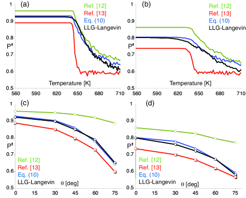
Figure 1: Comparison between macrospin models and mean field atomistic LLG-Langevin simulations. Results have been averaged over $4096$ particles. The percentage of particles ($P^{\uparrow}$) for which $\mbox{\boldmath${M}$}\cdot\mbox{\boldmath${H}$}_{w}>0$ is shown as a function of temperature during a cooling process $T[K]=300+450\times\exp(-t/\tau)$, with timescale $\tau=1ns$ in panel (a), and $\tau=100ps$ in panel (b). The write probability, i.e. $P^{\uparrow}(T\ll T_{c})$, is shown as a function of field angle ($\theta$ measured at $0^{\circ},30^{\circ},45^{\circ},60^{\circ},75^{\circ}$) when the time-scale is $1ns$ in panel (c), and $100ps$ in panel (d). $H_{w}=5kOe$ everywhere.

In Figure 1 panel (a) we compare the macrospin models, Ref.Evans:2012vn /Ref.Xu:2012fk /Eq. (10) in green/red/blue, with atomistic LLG-Langevin simulations (black) for $H_{w}=5kOe,\theta=0^{\circ},\tau=1ns$. As the temperature decreases, the angular diffusion model from Ref.Xu:2012fk (red) predicts virtually no change in $P^{\uparrow}$, until the Curie point is reached, where $P^{\uparrow}$ increases sharply before freezing. On the other hand, the stochastic LLB model from Ref. Evans:2012vn (green) qualitatively recovers the smooth transition near $T_{c}$ seen from the atomistic simulations. The new stochastic LLB model in Eq. (10) (blue) recovers the features of the atomistic simulations both qualitatively and quantitatively. The same behavior is observed in panel (b), where the time-scale $\tau$ is reduced to $100ps$. In this case the model from Ref. Evans:2012vn (green) significantly deviates from the atomistic simulation. Panels (c) and (d) show the dependence of the write probability, $P^{\uparrow}(T\ll T_{c})$, with field angle $\theta$, for the time-scales $\tau=1ns$ and $\tau=100ps$ respectively. Good agreement between Eq. (10) and the atomistic simulations is found for all cases.

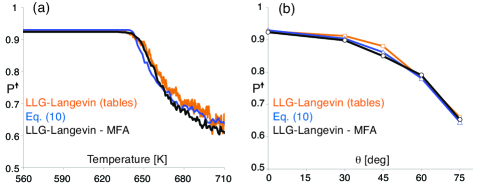
Figure 2: Comparison between the new macrospin model in Eq. (10) and atomistic LLG-Langevin simulations, both with and without the mean field approximation. Results for the macrospin and mean-field atomistic simulations have been averaged over $4096$ particles. Results for the atomistic calculations without the MFA have been averaged over $1024$ particles. The percentage of particles ($P^{\uparrow}$) for which $\mbox{\boldmath${M}$}\cdot\mbox{\boldmath${H}$}_{w}>0$ is shown as a function of temperature during a cooling process $T[K]=300+450\times\exp(-t/\tau)$, with timescale $\tau=1ns$ in panel (a). The write probability, i.e. $P^{\uparrow}(T\ll T_{c})$, is shown as a function of field angle ($\theta$ measured at $0^{\circ},30^{\circ},45^{\circ},60^{\circ},75^{\circ}$) in panel (b). $H_{w}=5kOe$ everywhere.

The LLB equation is used extensively to model systems for magnetic data storage, such as Heat-Assisted Magnetic Recording (HAMR)HAMR2 ; Lyberatos:2003zr ; HAMR1 and magneto-optical recordingStanciu:2007fk ; Mangin:2014ly . Current HAMR media employ FePt grains that contain more than $10^{4}$ unit cells. Even for future media with reduced grain-sizes, the number of unit cells can be expected to exceed $10^{3}$, sufficient to justify application of the central limit theorem in deriving the macrospin distribution [Eq. (5)]. However, the underlying assumption that the mean field and temperature are constant across the magnetic grain, is weaker. For example, for unit cells on the surface of the grain the overall magnetic field can be considerably smaller because there are fewer neighboring atoms to interact with. For systems where the number of surface unit cells is comparatively large, that is for small or irregularly-shaped grains, this effect becomes significant. Moreover, temperature variations within the grain influence the strength of the exchange and anisotropy fields, thereby undermining the accuracy of the macrospin model. The mean field approximation also precludes the excitation of internal modes of the grain that reflect the properties of the exchange interaction. Atomistic models can be used to lift the restrictions due to the mean field approximation, and they offer the flexibility of modeling heterogenous magnetic materials, albeit at considerable computational cost.

To examine the applicability of the mean field theory we compare the new macrospin model [Eq. (10)] and the mean field atomistic simulations with a fully atomistic model in Figure 2. For the fully atomistic simulations the magnetic field $\mbox{\boldmath${H}$}_{i}$ at each lattice point is calculated from the spin Hamiltonian: $\mbox{\boldmath${H}$}_{i}=\partial\mathcal{H}/\partial\mbox{\boldmath${S}$}_{i}$, where $\mathcal{H}=-\sum_{i\neq j}\mbox{\boldmath${S}$}_{i}\cdot\mbox{\boldmath${J}$}_{ij}^{M}\cdot\mbox{\boldmath${S}$}_{j}-\sum_{i}(k_{Fe}^{(0)}+m_{i}K^{\prime})(\mbox{\boldmath${S}$}_{i}\cdot\hat{\mbox{\boldmath${e}$}}_{z})^{2}-\mu_{0}\mbox{\boldmath${H}$}_{w}\cdot\sum_{i}\mbox{\boldmath${S}$}_{i}$. The tensor $\mbox{\boldmath${J}$}_{ij}^{M}$ describes the exchange interactions with $8\times 8\times 6\times 2=768$ terms, $k_{Fe}^{(0)}=-0.097meV$, $K^{\prime}=0.0223meV$, and $m_{i}$ is the number of nearest neighbors at each lattice pointALyberatos . The simulation parameters and conditions were the same as those described in Figure 1 for the time-scale $\tau=1ns$. The results from the fully atomistic simulations have been averaged over $1024$ particles and are shown in Figure 2 with orange lines. Panels 2(a) and 2(b) correspond to 1(a) and 1(c) and confirm that there is good agreement between Eq. (10) and the fully atomistic simulations for all cases.

We have developed a stochastic Landau-Lifshitz-Bloch equation [Eq. (10)] for single-domain magnetic particles, in which the stationary state is determined directly from the underlying atomic spin equilibrium and the stochastic process is a mean-reverting random walk. At room temperature the stochastic behavior reduces to angular diffusion in agreement with the stochastic LLG equation. The angular diffusion coefficient increases linearly with temperature before saturating at $T_{c}$. Diffusion in the magnetization magnitude increases rapidly with temperature when $T\lesssim T_{c}$ and saturates at $T_{c}$. The stochastic LLB model is in excellent agreement with mean-field atomistic LLG-Langevin simulations and is immediately applicable for modeling a variety of magnetic systems.

References

- [1] Ernst Ising. Beitrag zur theorie des ferromagnetismus. Zeitschrift für Physik, 31(1):253–258, 1925.
- [2] R. E. Watson, M. Blume, and G. H. Vineyard. Spin motions in a classical ferromagnet. Physical Review, 181(2):811–823, 05 1969.
- [3] U. Nowak, O. N. Mryasov, R. Wieser, K. Guslienko, and R. W. Chantrell. Spin dynamics of magnetic nanoparticles: Beyond brown’s theory. Physical Review B, 72(17):172410–, 11 2005.
- [4] R F L Evans, W J Fan, P Chureemart, T A Ostler, M O A Ellis, and R W Chantrell. Atomistic spin model simulations of magnetic nanomaterials. Journal of Physics: Condensed Matter, 26(10), 2014.
- [5] R. H. Victora and Pin-Wei Huang. Simulation of heat-assisted magnetic recording using renormalized media cells. IEEE Trans. on Magn., 49(2):751–757, February 2013.
- [6] D. A Garanin. Generalized equation of motion for a ferromagnet. Physica A: Statistical Mechanics and its Applications, 172(3):470–491, 4 1991.
- [7] D. A. Garanin. Fokker-planck and landau-lifshitz-bloch equations for classical ferromagnets. Physical Review B, 55(5):3050–3057, 02 1997.
- [8] Lifshitz E. M. Landau L. D. On the theory of the dispersion of magnetic permeability in ferromagnetic bodies. Phys. Zeitsch. der Sow., 8:153–169, 1935.
- [9] F. Bloch. Nuclear induction. Physical Review, 70(7-8):460–474, 10 1946.
- [10] William Fuller Brown. Thermal fluctuations of a single-domain particle. Physical Review, 130(5):1677–1686, 06 1963.
- [11] D. A. Garanin and O. Chubykalo-Fesenko. Thermal fluctuations and longitudinal relaxation of single-domain magnetic particles at elevated temperatures. Physical Review B, 70(21):212409, 12 2004.
- [12] R. F. L. Evans, D. Hinzke, U. Atxitia, U. Nowak, R. W. Chantrell, and O. Chubykalo-Fesenko. Stochastic form of the landau-lifshitz-bloch equation. Physical Review B, 85(1):014433, 01 2012.
- [13] Lei Xu and Shufeng Zhang. Magnetization dynamics at elevated temperatures. Physica E: Low-dimensional Systems and Nanostructures, 45(0):72–76, 8 2012.
- [14] Lei Xu and Shufeng Zhang. Self-consistent bloch equation and landau-lifshitz-bloch equation of ferromagnets: A comparison. Journal of Applied Physics, 113(16):163911, 2013.
- [15] J.-G. Zhu and Hai Li. Understanding signal and noise in heat assisted magnetic recording. IEEE Trans. on Magn., 49(2):765–772, February 2013.
- [16] L. Néel. Théorie du traînage magnétique des ferromagnétiques en grains fins avec applications aux terres cuites. Ann. Géophys, 5:99–136, 1949.
- [17] Kittel C. Introduction to Solid State Physics. Wiley, 8 edition, 2005.
- [18] D. Weller, Andreas Moser, Liesl Folks, Margaret E. Best, Wen Lee, M.F. Toney, M. Schwickert, J.-U. Thiele, and Mary F. Doerner. High ku materials approach to 100 gbits/in2. 10 IEEE Transactions on Magnetics, 36(1):10–15, January 2000.
- [19] Shouheng Sun, C. B. Murray, Dieter Weller, Liesl Folks, and Andreas Moser. Monodisperse fept nanoparticles and ferromagnetic fept nanocrystal superlattices. Science, 287(5460):1989–1992, 03 2000.
- [20] JoséLuis García-Palacios and Francisco J. Lázaro. Langevin-dynamics study of the dynamical properties of small magnetic particles. Physical Review B, 58(22):14937–14958, 12 1998.
- [21] S.R. Cumpson, P. Hidding, and R. Coehoorn. A hybrid recording method using thermally assisted writing and flux sensitive detection. IEEE Transactions on Magnetics, 36(5):2271 – 2275, September 2000.
- [22] A. Lyberatos and K. Yu Guslienko. Thermal stability of the magnetization following thermomagnetic writing in perpendicular media. Journal of Applied Physics, 94(2):1119–1129, 2003.
- [23] R.E. Rottmayer, Sharat Batra, D. Buechel, W.A. Challener, Julius Hohlfeld, Y. Kubota, Lei Li, Bin Lu, C. Mihalcea, Keith Mountfield, Kalman Pelhos, Chubing Peng, T. Rausch, Michael A. Seigler, D. Weller, and XiaoMin Yang. Heat-assisted magnetic recording. IEEE Transactions on Magnetics, 42(10):2417–2421, October 2006.
- [24] C. D. Stanciu, F. Hansteen, A. V. Kimel, A. Kirilyuk, A. Tsukamoto, A. Itoh, and Th. Rasing. All-optical magnetic recording with circularly polarized light. Physical Review Letters, 99(4):047601–, 07 2007.
- [25] S. Mangin, M. Gottwald, C-H. Lambert, D. Steil, V. Uhlíř, L. Pang, M. Hehn, S. Alebrand, M. Cinchetti, G. Malinowski, Y. Fainman, M. Aeschlimann, and E. E. Fullerton. Engineered materials for all-optical helicity-dependent magnetic switching. Nat Mater, 13(3):286–292, 03 2014.
- [26] A. Lyberatos. private communication.