Diagnosing Mass Flows Around Herbig Ae/Be Stars Using the He I $\lambda$10830 Line

Abstract

We examine He I $\lambda$10830 profile morphologies for a sample of 56 Herbig Ae/Be stars (HAEBES). We find significant differences between HAEBES and CTTSs in the statistics of both blue–shifted absorption (i.e. mass outflows) and red–shifted absorption features (i.e. mass infall or accretion). Our results suggest that, in general, Herbig Be (HBe) stars do not accrete material from their inner disks in the same manner as CTTSs, which are believed to accrete material via magnetospheric accretion, while Herbig Ae (HAe) stars generally show evidence for magnetospheric accretion. We find no evidence in our sample of narrow blue–shifted absorption features which are typical indicators of inner disk winds and are common in He I $\lambda$10830 profiles of CTTSs. The lack of inner disk wind signatures in HAEBES, combined with the paucity of detected magnetic fields on these objects, suggests that accretion through large magnetospheres which truncate the disk several stellar radii above the surface is not as common for HAe and late–type HBe stars as it is for CTTSs. Instead, evidence is found for smaller magnetospheres in the maximum red–shifted absorption velocities in our HAEBE sample. These velocities are, on average, a smaller fraction of the system escape velocity than is found for CTTSs, suggesting accretion is taking place closer to the star. Smaller magnetospheres, and evidence for boundary layer accretion in HBe stars, may explain the less common occurrence of red–shifted absorption in HAEBES. Evidence is found that smaller magnetospheres may be less efficient at driving outflows compared to CTTS magnetospheres.

1. INTRODUCTION

One of the most important aspects of pre–main sequence (PMS) stellar evolution is the interaction of the star with its surrounding environment. The rate at which the central object accretes and ejects material, stellar and circumstellar magnetic fields, and the geometry of the circumstellar environment all play an important role in the system’s evolution and the ultimate formation of planets. While many important details of a star’s interaction with its environment have been clarified for the low–mass PMS classical T–Tauri stars (CTTSs) (e.g. see Bouvier et al. 2007), much of the picture is still uncertain for the intermediate–mass PMS Herbig Ae/Be stars (hereafter HAEBES).

HAEBES are intermediate mass (2–10 ${\rm\,M_{\odot}}$) stars first classified by George Herbig in 1960 according to their A– or B–type emission line spectra and their association with, and illumination of, nebulosity (Herbig 1960). These criteria have since been adjusted by various authors in order to incorporate potential HAEBES that may have been excluded based on Herbig’s original criteria (e.g. Finkenzeller & Mundt 1984; Thé, de Winter, & Pérez 1994; Malfait et al. 1998). A decade after Herbig’s catalog was established, Strom et al. (1972) confirmed the pre–main sequence nature of HAEBES by showing that their surface gravities are lower than main sequence stars of the same spectral types. These observational results placed the HAEBES in the HR diagram above the zero–age main sequence of theoretical evolutionary tracks (e.g. those of Iben 1967), further suggesting the young age of these objects. The youth of HAEBES has since been confirmed by multiple studies (e.g. Palla & Stahler 1991; van den Ancker et al. 1998).

The analogy with CTTSs motivated Herbig’s search for the higher mass HAEBES. In general, HAEBES and CTTSs have a number of observed features in common, most notably infrared excesses indicating circumstellar material (Bertout et al. 1988; Hillenbrand et al. 1992; Mannings & Sargent 1997; Natta et al. 2001; Meeus et al. 2001) and, in the case of CTTS and some HAEBES, excess UV/optical luminosity attributed to mass accretion onto the star (e.g. Garrison 1978; Basri & Batalha 1990; Hartigan et al. 1991; Böhm & Catala 1995; Donehew & Brittain 2011). Strong emission lines, both permitted and forbidden, are also common to both groups (Finkenzeller 1985; Edwards et al. 1987; Hamann & Persson 1992; Böhm & Catala 1994; Hartigan et al. 1995; Corcoran & Ray 1997; Alencar & Basri 2000). We note that there are currently no specific criteria differentiating between distinct PMS evolutionary phases for HAEBES as there is for the TTSs (CTTSs vs weak line TTSs, or WTTSs), although the idea of HAEBES representing an evolutionary sequence has been outlined in several studies (e.g. Corcoran & Ray 1997; van den Ancker et al. 1997; Malfait et al. 1998). Thus we consider HAEBES as a single group even though observed features can vary widely from star to star and a continuum of evolutionary stages is most likely present within any large HAEBE sample. Although HAEBES share many observed properties with CTTSs, it is still unclear as to the extent to which HAEBES interact with their circumstellar environments in ways similar to CTTSs.

The presence of circumstellar disks around many HAEBES is now well established (e.g. Grady et al. 2000; Natta et al. 2001; Dent et al. 2005; Eisner et al. 2007; Matter et al. 2014). There is also significant evidence that many HAEBES are actively accreting material from their disks (Donehew & Brittain 2011; Mendigutía et al. 2011, 2012). The strong Balmer lines and excess UV/optical continuum emission in CTTSs are generally accepted to be produced by accreting disk material that falls to the surface along magnetic field lines from a truncation point in the disk at several stellar radii above the star (Bouvier et al. 2007). This scenario, termed magnetospheric accretion (MA), can account for many of the observed properties and spectral features in CTTSs (Edwards et al. 1994; Hartmann et al. 1994; Calvet & Gullbring 1998; Muzerolle et al. 1998, 2001). In addition, strong magnetic fields, which are required in order for MA to occur, are ubiquitous on TTSs (e.g. Johns–Krull 2007). Magnetospheric accretion has also been used to explain accretion signatures in some HAEBES (Muzerolle et al. 2004; Grady et al. 2010). Mendigutía et al. (2011) calculated accretion rates for a large sample of HAEBES by assuming that MA operates in these systems.

It is unclear, however, that MA is the dominant accretion mechanism in HAEBES. Perhaps the largest uncertainty regarding MA in HAEBES is the current lack of detected magnetic fields on these objects. Wade et al. (2007) analyzed 50 HAEBES using low–resolution spectropolarimetry and found only 8–12% of their sample to have detectable magnetic fields. They also place an upper limit of 300 G on the longitudinal fields of the undetected sample. More recently, Alecian et al. (2013) performed a high–resolution spectropolarimetric study of 70 HAEBES. The high resolution of their data provided greater sensitivity to Zeeman signatures, enabling detection of weak longitudinal fields. Their results include the confirmation of 5 magnetic HAEBES while only one new object (HD 35929) is reported as magnetic. Although the magnetic field strengths predicted for MA to operate around HAEBES are closer to $\sim$a few hundred gauss (Wade et al. 2007), as opposed to the kilogauss fields required for low mass stars, the lack of significant detections of any magnetic fields on a large majority of these objects, many of which shows signs of active accretion, suggests a different accretion mechanism is mediating the transfer of mass from the disk to the star. Since outflows around young stars are known to be correlated with accretion (Hartigan et al. 1995), a shift from MA to a different accretion mechanism may impact the type and strength of outflowing material as well.

The focus of this study is to probe the inner accretion and wind launching regions using the He I $\lambda$10830 Å line diagnostic, which has been successfully employed for similar studies of CTTSs (e.g. Dupree et al. 2005; Edwards et al. 2006) as well as in mass loss studies of Wolf–Rayet stars (Howarth & Schmutz 1992) and classical Be stars (Groh et al. 2007). In this paper we present high spectral resolution observations of the He I $\lambda$10830 line for a sample of 56 HAEBES. The He I $\lambda$10830 diagnostic is an excellent tracer of outflowing material due to its metastable lower level, i.e. unless the electron density is sufficiently high for collisional de–excitation to be important, the atoms tend to remain in the lower 2s$\>{}^{3}S$ energy level until a photon is absorbed (see Kwan & Fischer 2011, for details on the atomic data). Thus, He atoms excited into the lower energy level have the ability to trace the full velocity extent of the material. Section 2 provides a brief overview of HAEBE magnetic fields and how these fields potentially mediate accretion and outflows. In §3 we discuss our observations and data reduction procedures. The line profiles and their morphology classifications are given in §3. The incidence of red and blue–shifted absorption features in our sample is also presented in §3. The line profiles are examined and analyzed in §5 within the context of disk or stellar winds and mass infall. In §5 we also elaborate on the implications of our observations for HAEBES as a whole, as well as discuss scenarios potentially responsible for the differences in morphology statistics observed between HAEBES and CTTSs. A summary of our findings and conclusions are presented in §6.

2. MAGNETIC FIELDS: MAGNETOSPHERIC ACCRETION AND OUTFLOWS

As mentioned in §1, magnetic fields have only been confirmed on a handful of HAEBES (Wade et al. 2007; Alecian et al. 2013) while kilogauss strength magnetic fields seem to be ubiquitous on CTTSs (Johns–Krull 2007). Wade et al. (2007) pointed out that the required surface dipolar field strength for magnetospheric accretion to occur on a typical HAEBE, according to the MA theories of Königl (1991) and Shu et al. (1994), is a few hundred gauss, much lower than the kilogauss fields required for CTTSs. Although a large majority of HAEBES do not have confirmed magnetic fields, most of the attempted measurements have been performed using polarimetry. The uncertainties of these measurements are large, often tens to hundreds of Gauss (Wade et al. 2007; Alecian et al. 2013). For polarimetric measurements of magnetic fields on CTTSs the detected longitudinal fields are of the order $\sim$100 G (e.g. Donati et al. 2010, 2011, 2011a) while Zeeman broadening measurements reveal strong average fields of $\sim$2 kG (Johns–Krull 2007). For the objects in our sample with measured $\dot{M}$, $R_{*}$, $M_{*}$, and $v$sin$i$ we have calculated the predicted mean surface equatorial magnetic field strength using the theory of Shu et al. (1994). The median field strength for our sample is 470 G, about a factor of 4 lower than for CTTSs. Thus the longitudinal fields measured via polarimetry may simply be too low to detect under current observational constraints. Zeeman broadening measurements for HAEBES would provide better constraints on the surface magnetic field strengths. However, the high $v$sin$i$ values of HAEBES and fewer number of photospheric absorption lines compared to CTTS makes Zeeman broadening detections very difficult. In any case, we cannot rule out MA on HAEBES based on the lack of detected fields; the field strengths, although large enough to produce MA flows, may simply be too weak to detect using current methods and instrumentation.

Muzerolle et al. (2004) pointed out that if MA is operating on some HAEBES then the large $v$sin$i$ values for many stars would force the corotation radii to be very small ($\sim$2 $R_{*}$), outside of which accretion cannot take place (Shu et al. 1994). Small corotation radii, or truncation radii, result in smaller magnetospheres around HAEBES compared to CTTSs. We note that “smaller” in this case refers to the volume of the MA flow where the flow kinematics are dominated by the magnetic field. Thus smaller magnetospheres are, in general, required in order for MA to operate around HAEBES. We test this prediction observationally in §5.1.2.

Since smaller corotation radii, and in turn smaller magnetospheres, are expected for HAEBES experiencing MA, the question arises: can magnetocentrifugal winds be driven by small magnetospheres? Numerical simulations have shown that CTTS magnetospheres can drive strong outflows from the magnetosphere–disk interaction region (e.g. Kurosawa & Romanova 2012; Zanni & Ferreira 2013) and this behavior is expected from analytic MA theories Shu et al. (1994); Mohanty & Shu (2008). For a wind being driven along a magnetic field line, the field enforces corotation out to approximately the Alfvén radius, $R_{A}$. Thus inside $R_{A}$ the velocity of the outflowing gas is $v_{g}$($r$)=$v$sin$i$($r/R_{*}$) if we take $v$sin$i$ to be the approximate rotation velocity of the field line anchored to star. If we assume that the escape velocity at $R_{A}$ is approximately the velocity of the gas at $R_{A}$, we can estimate $R_{A}$/$R_{*}$=[$2GM_{*}$/($v$sin$i^{2}$$R_{*}$)]^1/3. We note that here $R_{A}$/$R_{*}$ differs from the corotation radius in the disk, $R_{co}$/$R_{*}$, by a factor of 2^1/3. The large $v$sin$i$ values of HAEBES, and thus the small corotation radii, will generally result in smaller values of $R_{A}$ in HAEBES than in CTTSs. We will also investigate the difference in $R_{A}$ between HAEBES and CTTSs in §4.4.

3. OBSERVATIONS AND DATA REDUCTION

Our sample of HAEBES (Table 1) consists of 56 objects chosen from the catalogues of Viera et al. (2003); Thé, de Winter, & Pérez (1994); and Finkenzeller & Mundt (1984). Classification as a HAEBE was the only criteria for being included in our sample. As a result, our sample covers a wide range of spectral types, from B0 to F2. Our objects most likely cover a wide range in evolutionary status. The evolutionary implications of our He I $\lambda$10830 observations will be discussed in §4. While this broad selection criteria makes it difficult to make specific comparisons between groups with distinct observational properties, it is sufficient for reaching general conclusions about HAEBES as a whole. Physical parameters for our sample are given in Table 2. With the exception of the radial velocity for some objects, the Table 2 values are taken from the literature sources indicated in column 10.

Table 1Log of He I $\lambda$10830 observations

Object ID	Instrument	Telescopea	UT Date	Integration timeb (s)	Co–added spectra	Final S/Nc
(1)	(2)	(3)	(4)	(5)	(6)	(7)
AB Aur	GNIRS	GN	14–Dec–2012	60	12	160
BD+41 3731	Phoenix	KP2.1	12–Nov–2013	600	8	15
BD+61 154	Phoenix	KP4	03–Mar–2013	800	4	15
BF Ori	Phoenix	KP4	02–Mar–2013	800	4	20
CQ Tau	Phoenix	KP4	27–Feb–2013	600	4	50
DW CMa	Phoenix	KP4	02–Mar–2013	600	8	10
HBC 548	Phoenix	KP2.1	08–Nov–2013	600	2	5
HD 114981	GNIRS	GN	16–Jan–2013	180	8	175
HD 141569	Phoenix	KP4	27–Feb–2013	600	6	55
HD 142666	Phoenix	KP4	27–Feb–2013	750	4	30
HD 144432	Phoenix	KP4	28–Feb–2013	600	6	90
HD 163296	Phoenix	KP4	28–Feb–2013	600	2	200
HD 17081	Phoenix	KP4	03–Mar–2013	90	2	95
HD 190073	Phoenix	KP2.1	08–Nov–2013	600	4	65
HD 200775	Phoenix	KP4	27–Feb–2013	300	2	20
HD 244604	Phoenix	KP4	28–Feb–2013	600	4	20
HD 250550	Phoenix	KP4	27–Feb–2013	700	4	35
HD 287823	Phoenix	KP4	02–Mar–2013	600	4	10
HD 34282	Phoenix	KP4	01–Mar–2013	800	4	10
HD 34700	Phoenix	KP4	27–Feb–2013	600	2	100
HD 35187	GNIRS	GN	14–Dec–2012	110	2	125
HD 36408	GNIRS	GN	21–Dec–2012	65	4	290
HD 37490	GNIRS	GN	13–Dec–2012	30	8	15
HD 38120	Phoenix	KP2.1	09–Nov–2013	600	4	25
HD 50083	GNIRS	GN	13–Dec–2012	90	8	215
HD 52721	GNIRS	GN	13–Dec–2012	65	8	120
HD 53367	Phoenix	KP4	02–Mar–2013	300	2	80
HK Ori	Phoenix	KP2.1	08–Nov–2013	600	4	15
IL Cep	Phoenix	KP2.1	09–Nov–2013	600	4	25
IP Per	Phoenix	KP4	28–Feb–2013	800	5	15
IRAS 15462–2551 S	Phoenix	KP4	27–Feb–2013	800	4	10
LkH$\alpha$ 215	Phoenix	KP4	01–Mar–2013	800	2	15
MWC 1080	Phoenix	KP2.1	10–Nov–2013	600	8	35
MWC 120	GNIRS	GN	17–Dec–2012	140	4	165
MWC 137	Phoenix	KP4	28–Feb–2013	600	2	5
MWC 480	GNIRS	GN	13–Dec–2012	105	8	135
MWC 610	Phoenix	KP2.1	09–Nov–2013	600	4	50
MWC 614	Phoenix	KP2.1	10–Nov–2013	600	4	75
MWC 758	GNIRS	GN	13–Dec–2013	145	8	160
MWC 863	Phoenix	KP4	28–Feb–2013	600	4	95
MWC 953	Phoenix	KP4	28–Feb–2013	600	2	50
T Ori	Phoenix	KP4	01–Mar–2013	800	4	15
UX Ori	Phoenix	KP4	27–Feb–2013	600	4	10
V1185 Tau	Phoenix	KP2.1	09–Nov–2013	600	2	10
V1578 Cyg	Phoenix	KP2.1	11–Nov–2013	600	4	15
V1685 Cyg	Phoenix	KP2.1	08–Nov–2013	600	3	20
V1977 Cyg	Phoenix	KP2.1	14–Nov–2013	600	8	10
V346 Ori	Phoenix	KP2.1	08–Nov–2013	600	4	10
V351 Ori	Phoenix	KP4	01–Mar–2013	800	2	20
V374 Cep	Phoenix	KP2.1	09–Nov–2013	600	6	30
V380 Ori	Phoenix	KP4	03–Mar–2013	800	2	15
V718 Sco	Phoenix	KP4	27–Feb–2013	600	4	45
V791 Mon	Phoenix	KP4	03–Mar–2013	800	4	20
VY Mon	Phoenix	KP4	03–Mar–2013	1200	8	5
XY Per	Phoenix	KP2.1	08–Nov–2013	600	4	40
Z CMa	GNIRS	GN	15–Dec–2012	90	8	130

Table 2HAEBE sample physical parameters

		$v_{rad}$	$M_{*}$	$R_{*}$	vsini	log($\dot{M}$)	Disk	i
Object ID	Spectral Type	(km s-1)	(${\rm\,\it{M_{\odot}}}$)	(${\rm\,\it{R_{\odot}}}$)	(km s-1)	(M⊙ yr-1)	Detected	(∘)	Referencesa
(1)	(2)	(3)	(4)	(5)	(6)	(7)	(8)	(9)	(10)
AB Aur	A0	24.7	2.50	2.62	116	-6.85	Y	40	1,2,7
BD+41 3731	B5	-14.0	5.50	3.80	345	$\cdots$	N	$\cdots$	1,8
BD+61 154	B8	-16.0	3.40	2.42	112	$\cdots$	Y	70	1,6,9
BF Ori	A2	22.0	2.58	3.26	39	$<$-8.00	Y	$\cdots$	1,2,6,8
CQ Tau	F2	35.7	2.93	5.10	98	$<$-8.30	Y	29	1,2,12,37
DW CMa†	B3	$\cdots$	$\cdots$	$\cdots$	$\cdots$	$\cdots$	Y	$\cdots$	4,13
HBC 548†	B9	$\cdots$	3.80	3.20	$\cdots$	$\cdots$	Y	$\cdots$	6
HD 114981	B5	-50.0	7.90	7.00	239	$\cdots$	N	$\cdots$	1
HD 141569	A0	35.7	2.33	1.94	228	-6.90	Y	55	1,2,14
HD 142666	A5	-7.0	2.15	2.82	65	-7.22	Y	$\cdots$	1,3,15
HD 144432	A7	-3.0	1.95	2.59	79	$<$-7.22	Y	$\sim$30	1,2,16,17
HD 163296	A1	-9.0	2.23	2.28	129	-7.16	Y	$\cdots$	1,3,6,18
HD 17081	B8	11.5	4.65	4.84	20	$\cdots$	N	$\cdots$	1,27,33
HD 190073	A1	0.2	2.85	3.60	4	$\cdots$	Y	45	1,19
HD 200775	B4	-23.3	10.70	10.4	26	$\cdots$	Y	55	1,20
HD 244604	A4	26.8	2.66	3.69	98	-7.20	Y	$\cdots$	1,3,21
HD 250550	B8	-22.0	4.80	3.50	79	-7.80	Y	$\cdots$	1,3,13
HD 287823	A0	-0.3	2.50	2.60	10	$\cdots$	?	$\cdots$	1
HD 34282	A3	16.2	1.59	1.66	105	$<$-8.30	Y	$\cdots$	1,2,18,22
HD 34700	F9	21.0	2.40	4.20	46	-8.30	Y	$\cdots$	2,23
HD 35187	A2	27.0	1.93	1.58	93	-7.60	Y	$\cdots$	1,3,24
HD 36408	B8	15.0	4.10	3.50	$\cdots$	$<$-8.00	?	$\cdots$	2
HD 37490	B4	21.0	$\cdots$	$\cdots$	180	$\cdots$	N	$\cdots$	6,25,26
HD 38120	B9	28.0	2.49	1.91	97	-6.90	Y?	$<$8	1,3,35
HD 50083	B4	-0.5	12.10	10.0	233	$\cdots$	?	$\cdots$	1
HD 52721	B3	21.0	9.10	5.00	215	$\cdots$	N	$\cdots$	1,6
HD 53367	B1	47.2	16.10	7.10	41	$<$-8.92	N	$\cdots$	1,3,6
HK Ori	A3	14.4	3.00	4.10	60	-5.24	Y	$\cdots$	2,6
IL Cep	B4	-39.0	$\cdots$	$\cdots$	179	$\cdots$	?	$\cdots$	1
IP Per	A3	13.7	1.86	2.10	80	$\cdots$	?	$\cdots$	1
IRAS 15462-2551 S†	A5	$\cdots$	$\cdots$	$\cdots$	$\cdots$	$\cdots$	Y	90	4,27
LkH$\alpha$ 215	B7	0.1	5.8	5.9	210	$\cdots$	N?	$\cdots$	1,6,10,13
MWC 1080†	B1	$\cdots$	17.4	7.3	$\cdots$	$\cdots$	Y	83	1,6,10
MWC 120	B9	47.0	3.94	4.60	120	-6.85	Y	$\cdots$	1,3,
MWC 137†	B1	$\cdots$	$\cdots$	$\cdots$	$\cdots$	$\cdots$	Y	80	6,10,13
MWC 480	A4	12.9	1.93	1.93	98	$<$-7.23	Y	37	1,2,12
MWC 610	B3	14.0	8.00	4.70	219	$\cdots$	?	$\cdots$	1
MWC 614	A0	15.1	$\cdots$	$\cdots$	$\cdots$	-6.59	Y	$\cdots$	3,28
MWC 758	A5	17.8	2.90	4.40	54	-6.05	Y	21	1,3,12
MWC 863	A1	-5.0	2.56	2.89	108	-6.12	Y	38	1,2,29
MWC 953	B3	23.0	$\cdots$	$\cdots$	$\cdots$	$\cdots$	?	$\cdots$	5
T Ori	A3	56.1	3.13	4.47	147	-6.60	Y	$\cdots$	1,2,30
UX Ori	A1	12.0	6.72	12.1	221	-7.18	Y	$<$8	1,3,6,35
V1185 Tau	A2	1.0	2.04	1.75	250	$\cdots$	?	$\cdots$	1
V1578 Cyg	A1	-3.0	5.90	9.70	199	$\cdots$	Y	$\cdots$	1,6
V1685 Cyg†	B4	-16.0	$\cdots$	$\cdots$	$\cdots$	$\cdots$	Y	41?	30,34
V1977 Cyg	B9	-13.0			$\cdots$	$\cdots$	?	$\cdots$	36
V346 Ori	A7	20.0	1.72	1.96	116	-6.90	N?	$\cdots$	1,3,35
V351 Ori	A6	15.0	2.88	4.38	100	$\cdots$	?	$\cdots$	1
V374 Cep†	B5	$\cdots$	$\cdots$	$\cdots$	$\cdots$	$\cdots$	?	$\cdots$	$\cdots$
V380 Ori	B9	27.5	2.87	3.00	7	-5.60	Y	$\cdots$	1,3,6
V718 Sco	A4	-3.6	1.93	2.25	113	$\cdots$	Y?	32?	1,35
V791 Mon	B5	-2.6	$\cdots$	$\cdots$	$\cdots$	$\cdots$	?	$\cdots$	4
VY Mon†	B8	$\cdots$	$\cdots$	$\cdots$	$\cdots$	$\cdots$	Y	40	1,9
XY Per	A2	2.0	1.95	1.65	224	-7.02	?	$\cdots$	3
Z CMa	B9	-27.0	3.80	3.20	$\cdots$	-6.72	Y	$\cdots$	3,31

Note. — Stars with unknown radial velocities are marked with a $\dagger$.

3.1. Observations

Our observations were carried out using two instruments on three telescopes: GNIRS (11 objects) on Gemini North (Elias et al. 2006), and the Phoenix echelle spectrograph (Hinkle et al. 1998) (45 objects) on the Mayall 4 m and KPNO 2.1 m. Individual object observations are detailed in Table 1. Although the resolving power of GNIRS (R$\sim$18,000) is much lower than Phoenix (R$\sim$50,000), we found that almost all of the He I $\lambda$10830 features in our sample are broad and strong enough to be resolved at the lower resolution. Thus, little to no information is lost in the GNIRS spectra and similar mass flow scenarios can be investigated using both sets of data.

The GNIRS data was obtained in queue mode during the 2012B semester using the 0.10”x49” slit with the long camera and the 110 lines mm^-1 grating resulting in a velocity resolution of $\sim$17 km s^-1. Images were taken in nodded pairs with an offset of $\pm$10”. The X_G0518 order blocking filter was employed to isolate a single order around 1.1 $\mu$m providing wavelength coverage from 1.0678–1.0982 $\mu$m. Individual exposure times for the GNIRS sample ranged from 15.0–180.0 s yielding a typical S/N$\sim$150 for 4–6 co–added exposures. Telluric standards at a similar airmass were observed immediately before or after each object. Arc lamp exposures were obtained for wavelength calibration purposes.

The Phoenix observations were obtained during three separate runs in 2013. The 4–pixel slit was used which corresponds to 0.7”x28” at the Mayall 4m and 1.4”x56” at the KPNO 2.1 m. The grating was configured to provide wavelength coverage from 1.0810–1.0860 $\mu$m and the J9232 order blocking filter was used to eliminate light from any overlapping orders. This setup yields a velocity resolution of $\sim$6 km s^-1 at either telescope. Spectroscopic standards were obtained for the entire range of HAEBE spectral types; telluric standards were obtained at a variety of airmasses. ThArNe lamp exposures were taken in order to provide wavelength calibrations. Signal–to–noise ratios varied significantly for the Phoenix sample depending on the combination of object brightness and the telescope used for the observation. Almost all 2.1 m targets required 4x900s observations in order to achieve a S/N$>$15, although the faintest objects have S/N$<$10. Repeating long exposure sequences for individual objects in order to boost the final S/N was avoided in order to obtain decent S/N exposures of more of the targets in our sample. This strategy was necessary to obtain quality observations of a large number of HAEBES. In any case, a low S/N spectrum is usually adequate for our purposes of identifying a He I $\lambda$10830 feature and measuring a reliable equivalent width. Marginal cases are noted as such in the discussion.

Figure 1.— Spectroscopic standard spectra for a sequence of spectral types. OH telluric absorption lines are marked near the 1.0832 and 1.0834 $\mu$m of the middle spectrum. Stellar absorption lines are generally weak and are highly doppler–broadened for large values of $v$sin$i$.

We note that the presence of sub–arcsecond companions, which appear to be common around HAEBES (e.g. Wheelwright et al. 2010), has a minimal effect on the analysis presented here. First, the large flux ratios of the HAEBE primaries to CTTS companions at 10830 Å ensures that absorption profiles are dominated by absorption of flux from the primary. Companion CTTS absorption profiles would be heavily veiled and, with the possible exception of the weak absorption features seen in a few spectra, would not be in agreement with the absorption strengths observed by Edwards et al. (2006) that rarely penetrate below 50% of the stellar continuum. A similar argument can be made concerning the strengths of the emission components. Thus any profile contributions from CTTS companions will likely be small perturbations on top of the primary HAEBE profile. In addition, the orbital separation of the binary would, in general, have to be very small in order to enable the absorption of flux from the primary by material emitted by the CTTS companion. Small physical separations of HAEBE binaries seem to be rare (Wheelwright et al. 2010) so these objects are unlikely to affect our analysis in this way.

3.2. Data Reduction

All of the data were reduced using custom IDL routines. Each pair of images was differenced and flat–fielded. The differenced spectra were then optimally extracted and co–added after being interpolated onto the same wavelength scale. Any remaining bad pixels were manually averaged between adjacent pixels. For objects observed at high airmass, a telluric standard was scaled and divided into the object spectrum in order to remove the atmospheric features, most importantly the OH absorption lines at $\sim$10832 and 10834 Å. These lines are present in each of the spectra shown in Figure 1 and are generally weak, even at high airmass. Any residual telluric absorption not removed by the telluric standard was masked using a quadratic estimate of the stellar spectrum across the narrow width of the OH telluric line. Third–order polynomial wavelength solutions were obtained by fitting the observed ThArNe lamp exposures using line identifications from Hinkle et al. (2001).

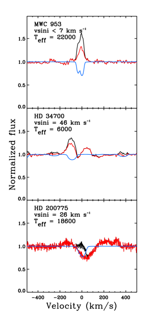
Figure 2.— He I $\lambda$10830 spectra of objects that required the removal of photospheric absorption features. The corrected spectrum is plotted in black, the observed spectrum in red, and the synthetic photosphere in blue.

In order to evaluate the contamination of photospheric absorption features, we employed both observed spectroscopic standards and synthetic spectra generated using SYNTHMAG (Piskunov 1999). A sample of our observed standards are shown in Figure 1. Many of our observed standards, which cover spectral types from B2 to F7, do not show any photospheric features. An overwhelming majority of our science targets also do not show any obvious photospheric lines. This is not unexpected: according to line lists extracted from VALD (Piskunov et al. 1995), there are few strong spectral lines ($\;\buildrel<\over{\sim}\;$0.90 of the continuum) in our observed wavelength range in A–type stars, the exception being Si I at $\lambda$10827 and 10843 and a S I line at $\lambda$10821 in the A6–7 objects. Photospheric He I lines only become prominent in $\sim$B5 stars and earlier. Most of our B–type objects are rotating so fast that the photospheric He I lines are broadened to the point of becoming negligible contributors to the spectrum. As a check, we visually examined the photospheric contribution of a broadened synthetic spectrum of similar $T_{eff}$ to each object. Out of the sample, only HD 34700, MWC 953, and HD 200775 were significantly altered by the subtraction of the synthetic spectrum. The result of this subtraction is shown in Figure 2. It can be seen that the profile morphology is not altered, i.e. the profile classification of these objects does not change. The low number of impacted objects is mainly a result of the moderate–to–high vsini values of our targets which tend to make the photospheric contributions weak compared to the circumstellar features. For the reasons stated above, the large majority of our sample does not require any removal of photospheric features and we are confident that the spectra presented in Figure 3 represent true contributions from the circumstellar environment. First–order normalization was performed using an average of the detector response along the columns on the detector where the spectra are located. This response function was measured using a median flat field from each night. Any residual slope was divided out using a linear fit.

4. LINE PROFILES

He I $\lambda$10830 line profiles for our sample are presented in Figure 3 and ordered according to morphology. To boost S/N and provide better clarity, 5–pixel ($\sim$6.9 km s^-1) binned spectra are plotted for the Phoenix observations. A number of measurements were made for each line profile, and these are provided in Table 3. The measurements contained in Table 3 are profile classification (column 3), the maximum blue and red–shifted line velocities (cols. 4 and 5), the velocity of peak emission and absorption (cols. 6 and 7), the line fluxes relative to the continuum at the peak emission and absorption velocities (cols. 8 and 9), and the blue and red equivalent widths (cols. 10 and 11). In general, our 56 objects can be categorized into six different morphology groups: 1. P–Cygni (PC–18 objects); 2. inverse P–Cygni (IPC–10 objects); 3. pure absorption (A–5 objects); 4. single–peaked emission (E–6 objects); 5. double–peaked emission (DP–6 objects); and 6. featureless (F–9 objects). Grouping of the few ambiguous profile morphologies (e.g. HD 35187, HD 34282) will not have a significant impact on the final morphology statistics. We note that the profiles of V374 Cep and MWC 137, listed as O for “other” in Figure 3 and Figure 4, do not neatly fit any of the profile categories given above. These are the only objects in our sample that display relatively strong, narrow absorption near the stellar rest velocity. These objects will not be included in the general profile descriptions of our sample and will be discussed briefly in §4.6. The number of objects in each morphology group, separated into Ae and Be stars, is shown in Figure 4. The featureless spectra will not be discussed in this section. We note that the signal–to–noise of the HBC 547, V1977 Cyg, and LkH$\alpha$ 215 observations are too low to rule out weak line signatures. For this same reason we treat them as featureless spectra. This choice does not significantly change the occurrence statistics of any one group of features.

Table 3HAEBE sample profile parameters

			$V_{max}^{blue}$	$V_{max}^{red}$	$V_{peak}^{em}$	$V_{peak}^{abs}$	$F_{peak}^{em}$	$F_{peak}^{abs}$	Wblue	Wred
Object ID	Spectral Type	Profile Typea	(km s-1)	(km s-1)	(km s-1)	(km s-1)	($F_{cont}$)	($F_{cont}$)	(Å)	(Å)
(1)	(2)	(3)	(4)	(5)	(6)	(7)	(8)	(9)	(10)	(11)
AB Aur	A0	PC	-175	405	185	-90	1.29	0.69	1.30	-1.70
BD+41 3731	B5	F	$\cdots$	$\cdots$	$\cdots$	$\cdots$	$\cdots$	$\cdots$	0.34	.27
BD+61 154	B8	PC	-350	300	25	-145	1.32	0.50	3.15	-1.19
BF Ori	A2	IPC	-385	285	-275	110	1.07	0.68	0.23	2.03
CQ Tau	F2	IPC	-490	130	-145	40	1.28	0.72	-2.24	0.78
DW CMa†	B3	A	-590	2	$\cdots$	-255	$\cdots$	0.35	8.92	$\sim$0
HBC 548†	B9	F	$\cdots$	$\cdots$	$\cdots$	$\cdots$	$\cdots$	$\cdots$	0.70	-0.20
HD 114981	B5	F	$\cdots$	$\cdots$	$\cdots$	$\cdots$	$\cdots$	$\cdots$	0.07	0.28
HD 141569	A0	F	$\cdots$	$\cdots$	$\cdots$	$\cdots$	$\cdots$	$\cdots$	0.04	0.07
HD 142666	A5	IPC	-310	150	-205	-35	1.15	0.70	0.28	0.66
HD 144432	A7	PC	-325	240	-10	-175	1.40	0.46	1.59	-1.58
HD 163296	A1	PC	-355	450	180	-80	1.27	0.61	1.35	-2.39
HD 17081	B8	F	$\cdots$	$\cdots$	$\cdots$	$\cdots$	$\cdots$	$\cdots$	0.17	0.04
HD 190073	A1	PC	-480	180	-30	-320	1.40	0.12	4.00	-1.36
HD 200775	B4	IPC	-200	355	-135	40	1.07	0.73	0.01	0.29
HD 244604	A4	PC	-290	260	35	-175	1.29	0.57	2.19	-1.25
HD 250550	B8	PC	-490	455	120	-275	1.56	0.30	4.70	-5.57
HD 287823	A0	F	$\cdots$	$\cdots$	$\cdots$	$\cdots$	$\cdots$	$\cdots$	0.12	0.24
HD 34282	A3	IPC	-300	300	-250	$\sim$0	1.09	0.75	0.58	1.54
HD 34700	F9	DP	-175	100	5	$\cdots$	1.22	$\cdots$	-0.61	-0.14
HD 35187	A2	DP	-350	390	205	10	1.11	0.81	0.26	-0.17
HD 36408	B8	A	-20	110	$\cdots$	45	$\cdots$	0.92	0.03	0.24
HD 37490	B4	DP	-305	290	-170	$\cdots$	1.17	$\cdots$	-1.04	-0.71
HD 38120	B9	PC	-325	365	90	-210	1.31	0.78	0.77	-2.31
HD 50083	B4	E	-190	290	70	$\cdots$	1.08	$\cdots$	-0.25	-0.48
HD 52721	B3	E	-185	310	-65	$\cdots$	1.06	$\cdots$	-0.34	-0.37
HD 53367	B1	DP	-300	165	30	$\cdots$	1.28	$\cdots$	-1.86	-1.04
HK Ori	A3	E	-310	120	30	$\cdots$	1.40	$\cdots$	-1.71	-0.75
IL Cep	B4	F	$\cdots$	$\cdots$	$\cdots$	$\cdots$	$\cdots$	$\cdots$	0.06	0.06
IP Per	A3	PC	-310	260	100	-240	1.44	0.77	1.24	-2.37
IRAS 15462-2551 S†	A5	IPC	-225	430	-45	162	1.58	0.57	-2.83	2.50
LkH$\alpha$ 215	B7	F	$\cdots$	$\cdots$	$\cdots$	$\cdots$	$\cdots$	$\cdots$	-0.07	-0.07
MWC 1080†	B1	PC	-530	465	150	-245	1.18	0.43	6.10	-1.68
MWC 120	B9	IPC	-245	370	-135	65	1.10	0.83	-0.42	0.32
MWC 137†	$\cdots$	$\cdots$	-180	550	100	55	6.48	0.57	-2.24	-18.8
MWC 480	A4	PC	-275	405	235	-125	1.27	0.42	4.25	-0.07
MWC 610	B3	DP	-275	160	-185	-10	1.03	0.94	-0.05	0.16
MWC 614	A0	DP	-250	230	-90	$\cdots$	1.16	$\cdots$	-0.87	-0.79
MWC 758	A5	PC	-360	415	145	-60	1.33	0.31	6.00	-2.38
MWC 863	A1	PC	-330	330	35	-105	1.25	0.73	0.63	-1.65
MWC 953	B3	E	-65	45	-5	$\cdots$	1.74	$\cdots$	-0.98	-0.48
T Ori	A3	E	-260	195	-80	$\cdots$	1.23	$\cdots$	-1.17	-0.46
UX Ori	A1	IPC	-230	150	-135	55	1.19	0.65	-0.54	1.34
V1185 Tau	A2	PC	-170	190	40	-120	1.23	0.74	0.92	-0.78
V1578 Cyg	A1	A	-170	120	-80	$\cdots$	$\cdots$	0.82	0.98	0.64
V1685 Cyg†	B4	E	-80	355	35	$\cdots$	1.25	$\cdots$	-0.30	-2.01
V1977 Cyg	B9	F	$\cdots$	$\cdots$	$\cdots$	$\cdots$	$\cdots$	$\cdots$	0.14	0.25
V346 Ori	A7	IPC	-300	320	-175	170	1.13	0.67	-0.28	0.67
V351 Ori	A6	PC	-325	280	-185	-15	1.07	0.87	-0.22	0.17
V374 Cep†	B5	$\cdots$	-350	445	145	10	1.40	0.19	-0.77	-1.68
V380 Ori	B9	PC	-220	245	5	-220	1.68	0.75	-0.94	-3.05
V718 Sco	A4	A	-155	205	$\cdots$	50	$\cdots$	0.46	1.07	2.49
V791 Mon	B5	PC	-480	320	20	-280	1.54	0.60	1.98	-3.42
VY Mon†	B8	PC	-445	340	90	-140	1.51	0.65	3.63	-2.87
XY Per	A2	IPC	-390	205	-230	20	1.12	0.62	-0.10	1.60
Z CMa	B9	A	-790	250	$\cdots$	-240	$\cdots$	0.51	7.46	0.89

Note. — Stars with unknown radial velocities are marked with a $\dagger$.

The red and blue–shifted absorption statistics for our sample, as well as those for the CTTS study of Edwards et al. (2006), hereafter EFHK, are given in Table 4. The 68% confidence intervals are calculated using Wilson’s score interval (Wilson 1927). The given percentage is the observed incidence and not the adjusted estimate given by Wilson’s test. We also employ contingency tests (see Feigelson & Babu 2012) to compare the number of red and blue absorption profiles observed in each group. Due to the small number statistics in most cases, we employ Fisher’s exact test for calculating the p–values. The null hypothesis in this case is that red–shifted and blue–shifted absorption features are equally as likely in both groups of objects. The p–value gives the probability of obtaining the observed distribution of profiles morphologies given the null hypothesis is true. Thus lower $p$–values indicate higher confidence in rejecting the null hypothesis. Table 5 displays the contingency tables and the results of the Fisher tests are shown in Table 6.

Table 4Statistical summary of absorption features

	This study				EFHK
	HAea	HBe	Total		CTTSs
	(1)	(2)	(3)		(4)
Red absorptionb	36%${}^{+9}_{-8}$	15%${}^{+10}_{-6}$	27%${}^{+7}_{-6}$		46%${}^{+8}_{-8}$
Blue absorption	36%${}^{+9}_{-8}$	45%${}^{+11}_{-10}$	40%${}^{+7}_{-7}$		69%${}^{+7}_{-8}$
Nietherc	28%${}^{+9}_{-8}$	40%${}^{+10}_{-10}$	33%${}^{+7}_{-6}$		10%${}^{+6}_{-4}$

The equivalent widths (EW) in columns (10) and (11) in Table 3 are calculated using the unbinned spectra. An estimate of the uncertainties in the equivalent widths can be gained by looking at the EW measurements for the featureless spectra. Typical EW uncertainties range from $\sim$2.0 Å for spectra with S/N$\sim$10 down to $\sim$0.1 Å for spectra with S/N$\sim$200. Radial velocity measurements (column 3 in Table 2) for most objects were taken from the literature. For objects which do not have previously determined radial velocities, we used shifted and rotationally broadened synthetic spectrum fits to high resolution optical spectra (data collected separately, Cauley & Johns–Krull 2014, in prep) to provide an estimate. For objects without identifiable photospheric features, we attempted gaussian fits to the wings of the H$\alpha$ emission profile. This method proved to be unreliable and these objects are analyzed without accounting for radial velocity. The 8 objects for which we do not have reliable RV estimates are indicated in Table 2 and Table 3. Interpretations of these object profiles are not significantly affected, assuming the RV values are not unreasonably high ($>\lvert 100\rvert$ km s^-1), which we do not see in the stars with known RVs.

Figure 3.— He I $\lambda$10830 line profiles for the objects listed in Table 1. Profiles are grouped according to morphology. The morphology abbreviation is given in the lower right hand corner of each plot window. Five–pixel binning is used to plot the objects observed with Phoenix. Spectral types are noted in the upper–right of each plot window. Objects that have potentially been misclassified as HAEBES (see §3.1) are marked with a $\star$ symbol next to their names. Note that the plot range has been narrowed for some objects with weak features.

Due to the importance of generating accurate statistics concerning the occurrence of mass accretion and wind flows around HAEBES, we discuss below (§4.1) the potential inclusion of objects in our sample that are not appropriate for comparison to CTTSs. It is important to note that although objects may be young (i.e. pre–main sequence) and thus correctly classified as a HAEBE, their inactivity or lack of interaction with their environments renders them irrelevant for comparing the methods by which HAEBES and CTTSs evolve. This is due to the fact that all CTTSs are accreting from their disks and the interaction of the star and disk is what produces the characteristic CTTS signatures. Thus HAEBES that are not surrounded by a close circumstellar accretion disk, and thus are non–accreting, are more similar to WTTSs, although there is currently no precise distinction between HAEBES with active disks and those without. Objects of this nature in our sample are excluded from most of the analysis. In sections 4.2–4.5 brief interpretations of the line profiles will be given along with the morphology descriptions. We will elaborate on the nature of the blue and red–shifted absorption profiles in §5.1.

4.1. Potentially misclassified objects

Based on the line profiles shown here and separately obtained H$\alpha$ profiles, as well as circumstellar disk indicators from the literature, we have identified 7 objects that may not be pre–main sequence stars. We note that classical Be stars often show featureless spectra or emission at He I $\lambda$10830 and the emission is often double–peaked (Groh et al. 2007). Discussions of the line profile morphology statistics will take these potential interlopers into account throughout this section and §5. There are two objects in our sample, HBC 548 and HD 141569, that have featureless spectra but also show evidence for circumstellar disks. HD 141569 appears to have significant grain growth in its disk and there is tentative evidence that a massive planet is present (Thi et al. 2014). It also shows significant evidence of accretion (Mendigutía et al. 2011). Thus although this object shows no evidence of activity at $\lambda$10830, its young age ($\sim$5 Myr) and the direct detection of warm molecular gas in its disk does not allow us to rule out its classification as a HAEBE. There is little information in the literature concerning the nature of the circumstellar material surrounding HBC 548 so we maintain its status as a HAEBE for our analysis. Objects not discussed in this section are assumed to be HAEBES that are interacting with their circumstellar environments.

4.1.1 BD+41 3731

This object has a featureless He I $\lambda$10830 spectrum. In addition, it shows a purely photospheric H$\alpha$ profile and no sign of a disk has been detected. Thé, de Winter, & Pérez (1994) in fact rejected this object as a HAEBE and Finkenzeller & Mundt (1984) also find little evidence for classification as a pre–main sequence object. Our observations add evidence to support its non–PMS nature and we suggest that it not be included as such in future studies.

4.1.2 HD 114981

HD 114981 was labeled as a HAEBE candidate by Viera et al. (2003) due to its H$\alpha$ emission and its detection in the IRAS Faint Source Catalogue. The spectrum at He I $\lambda$10830 is featureless and the H$\alpha$ profile shows a very symmetric, broad, double–peaked emission profile that is more similar to those found in rotating classical Be star disks than in the circumstellar environments of HAEBEs. It also has a very small $H-K$ excess ($\sim$0.03) indicating a lack of inner disk material. We suggest that this object is actually a classical Be star.

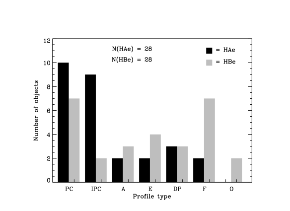
Figure 4.— Bar plot of the number of objects in each profile morphology category. The plot labels are the same as in Table 3. This plot includes the potentially misclassified objects from §3.1.

4.1.3 HD 17081

This star shows no features at He I $\lambda$10830. Dent et al. (2005) did not detect CO emission from HD 17081, indicating that it lacks a gaseous disk. In addition, the observations of Malfait et al. (1998) show that its IR excess begins at $\sim$12 $\mu$m making it closer to a Vega–type object that has completely dissipated the gas component of the disk and is left primarily with debris. Thus HD 17081 has most likely evolved past the point of accreting material from its surroundings, and probably lacks any significant close circumstellar disk.

4.1.4 HD 37490

This object shows no signs of a disk (Millan–Gabet et al. 2001) nor molecular material in its near vicinity (Fuente et al. 2002). The very symmetric double–peak at He I $\lambda$10830 matches the double–peaked H$\alpha$ profile. These line morphologies are very similar to those of a classical Be star, which is more likely the true nature of this object.

4.1.5 HD 52721

Hillenbrand et al. (1992) find no evidence of an IR excess around this object. Our observations show very weak, broad emission at He I $\lambda$10830; the H$\alpha$ emission profile is single–peaked, broad, and centered at the stellar rest velocity. The low vsini (21 km s^-1) suggests a small viewing angle which is consistent with single–peaked, centered emission at H$\alpha$ if the emission arises in classical Be disk. Thus this object is more likely a classical Be star than a HAEBE.

4.1.6 HD 53367

No IR excess was detected by Hillenbrand et al. (1992) around HD 53367. Furthermore, Pogodin et al. (2006) find significant evidence of a $\sim$20 ${\rm\,\it{M_{\odot}}}$ primary object in orbit with a $\sim$4–5 ${\rm\,\it{M_{\odot}}}$ secondary star. They conclude that the massive primary has already evolved onto (or beyond) the main sequence. By chance, we collected two spectra of this object separated by 9 months. The double–peaked nature of the emission line is present in both spectra with clear evidence that the peaks have shifted in velocity. Finally, the H$\alpha$ profile is well matched by two broad, relatively weak gaussian profiles suggesting two separate emission lines centered at different velocities. Thus our observations support the close binary scenario, indicating that the emission lines may not be an indicator of the age of the primary.

4.1.7 LkH$\alpha$ 215

There is mixed evidence for a disk surrounding LkH$\alpha$ 215. Hillenbrand et al. (1992) find a substantial IR excess past 1 $\mu$m that is typical of their Class I objects. Verhoeff et al. (2012), however, using higher resolution IR imaging, find that most of the IR flux is associated with the surrounding nebula and suggest that this object may instead be a classical Be star. No disk is detected at millimeter wavelengths by Alonso–Albi et al. (2009). Our featureless He I $\lambda$10830 spectrum is more consistent with the classical Be star scenario.

Given the uncertain nature of the 7 objects discussed above, we do not include them in the discussion below. We also recommend that they be excluded from any future HAEBE studies and that their classification be re–examined.

Table 5Contingency data

		HAe	HBe	Total		HAEBES	CTTS	Total
Red	Yes	10	3	13		13	18	30
absorption?	No	18	17	35		35	21	57
Blue	Yes	10	9	19		19	27	46
absorption?	No	18	11	29		29	12	41
	Total	28	20	48		48	39	87
		HAe	CTTS	Total		HBe	CTTS	Total
Red	Yes	10	18	28		3	18	21
absorption?	No	18	21	39		17	21	38
Blue	Yes	10	27	37		9	27	36
absorption?	No	18	12	30		11	12	23
	Total	28	39	67		20	39	59

Table 6Contingency test $p$–values

Feature	Groups	$p$–value
Red absorption	HAe vs. HBe	0.188
	HAEBES vs. CTTSs	0.076
	HAe vs. CTTSs	0.457
	HBe vs. CTTSs	0.023
Blue absorption	HAe vs. HBe	0.561
	HAEBES vs. CTTSs	0.009
	HAe vs. CTTSs	0.012
	HBe vs. CTTSs	0.094

4.2. P–Cygni profiles and blue absorption

Objects with P–Cygni (PC) profiles or blue absorption comprise 40%${}^{+7}_{-7}$ of our corrected sample. The Herbig Ae stars (HAe) show a 36%${}^{+9}_{-8}$ blue–shifted absorption incidence and the Herbig Be stars (HBe) show a 45%${}^{+11}_{-10}$ incidence. Table 6 shows there is a significant difference between the blue absorption incidence between CTTSs and both HAe and HBe stars. The blue–shifted absorption incidence in HAEBES as a whole is also significantly different from that in CTTSs. There is no signficant difference in the blue absorption incidence between HAe and HBe stars.

There are two objects (DW CMa and Z CMa) with strong blue absorption and no emission (classified as A type profiles). PC line profiles and broad blue–shifted absorption are classical indicators of outflows and are commonly found in the Balmer lines of many HAEBES (e.g. Finkenzeller & Mundt 1984; Viera et al. 2003). The blue absorption in many of our profiles extends out to terminal velocities near -400 – -500 km s^-1 with maximum depth velocities near $\sim$-200 km s^-1. The maximum blue velocities for DW CMa and Z CMa are much higher at $\sim$-600 and -800 km s^-1, respectively. Z CMa is a known binary consisting of a HAEBE and an FU Orionis–like object (e.g. Hinkley et al. 2013); DW CMa is an early B–star (Verhoeff et al. 2012). Both of these systems have strong wind signatures in the optical (Finkenzeller & Mundt 1984). The strong, extended He I $\lambda$10830 lines shown here confirm the strong outflows emerging from both systems. Four objects (AB Aur, HD 36112, IP Per, and MWC 758) show evidence of an emission bump near the maximum depth of the absorption profile.

There are two general types of PC profiles exhibited by our sample: I – (hereafter PCI) the peak of the emission component is red–shifted by $>$50 km s^-1 (e.g. AB Aur, MWC 480), and II – (hereafter PCII) the peak of the emission component is near (within 50 km s^-1) zero velocity (e.g. V380 Ori, HD 144432). Profiles PCI and PCII are split almost evenly across the PC objects. The equivalent widths of the absorption and emission components are approximately equal in 11 of 17 objects, while the absorption equivalent width is substantially larger in 5 of 17 profiles. The exception is V380 Ori for which the zero velocity–centered emission is much stronger than the blue–shifted absorption.

We note that the blue absorption signatures exhibited by the objects in this section are very broad and are more consistent with a stellar wind–like outflows than a broadened inner disk wind. Inner disk winds tend to produce narrower blue–shifted absorption profiles with relatively weak emission compared with stellar wind profiles (Kwan et al. 2007). In fact, our HAEBE sample shows no strong evidence of narrow, blue–shifted absorption indicating a lack of inner–disk winds in our sample. The larger rotational velocities expected for inner disk winds in HAEBES most likely cannot account for the observed broad, stellar wind–like profiles due to the narrow range of velocities projected against the stellar disk. Furthermore, disk winds have trouble reproducing the standard P-Cygni profiles observed in most of our PC objects (Kwan et al. 2007). One example supporting stellar winds over broadened disk winds in our sample is HD 190073 which has a $v$sin$i$ of $\sim$4 km s^-1 and an inclination angle of $\sim$45^∘, ruling out rotational broadening as the mechanism responsible for the broad absorption profile. Interpretations of the blue–shifted absorption profiles are given in §5.1.1. We will return to the lack of disk winds in our sample in §5.2.1.

4.3. Inverse P–Cygni profiles and red absorption

Inverse P–Cygni (IPC) profiles are formed through the scattering or absorption of photons by infalling material, producing red–shifted absorption features which are most easily detected when the absorption extends below the continuum. Our sample contains 13 objects, or 27%${}^{+7}_{-6}$ (Table 4) of the sample, that display IPC characteristics or red–shifted absorption (classified as ”A” type profiles) in their He I $\lambda$10830 profiles (e.g. CQ Tau, MWC 120). Interpretations of the red–shifted absorption profiles described here are presented in §5.1.2. Of these 13 objects, 10 are HAe stars and 3 are HBe stars. This corresponds to an incidence of 36%${}^{+9}_{-8}$ for the HAe objects and 15%${}^{+10}_{-6}$ for the HBe objects, indicating that MA is more common among HAe stars than HBe stars. A contingency test, however, shows (Table 6) that these percentages are not significantly different given the sample sizes. There is also no significant difference in the red absorption incidence between HAe stars and CTTSs. HBe stars show a significantly lower incidence than CTTSs. As a whole, the incidence of red–shifted absorption in HAEBES is significantly different from that in CTTSs.

The red–shifted absorption typically extends to $\sim$+200-250 km s^-1. The notable exception is IRAS 15462-2551 which displays broad, tapering absorption out to $\sim$+500 km s^-1. HD 34282 may have absorption that also extends to higher velocities but the continuum is noisy and difficult to locate. The red–shifted absorption in the profile of MWC 120 is superimposed on broad, weak emission that extends from -200 km s^-1 to +300 km s^-1. Similar behavior is exhibited by HD 200775, although the noise makes the extent of the emission less clear. Both of these objects have B spectral types.

Two of the 13 objects show only red–shifted absorption with no emission: HD 36408 and V718 Sco. HD 36408 shows weak, red–shifted absorption centered at +45 km s^-1. This signature may be due to a weak MA flow with a low surface filling factor viewed at a small inclination angle. This would be consistent with its relatively low accretion rate (Mendigutía et al. 2011). The profile of V718 Sco shows deep, asymmetric, slightly red–shifted absorption with relatively steep wings extending to -150 and +200 km s^-1. Evidence for accretion onto V718 Sco has been found in its Balmer lines (Guimarães et al. 2006) but no estimate exists for the accretion rate.

HD 142666, HD 34282, and V351 Ori all show IPC–type profiles but the maximum absorption is at slightly blue–shifted wavelengths. We include these objects in the IPC category since their emission components are clearly blue–shifted and the absorption is only marginally blue–shifted. Radial velocity estimates for these objects are accurate and cannot explain the blue–shifted maximum absorption depths. The profiles are entirely circumstellar since all of these objects are mid A–type stars and have no photospheric features near 10830 Å. These objects should be considered marginal IPC morphologies and follow up observations should be conducted to verify the line shapes.

4.4. Single–peaked emission

The six single–peaked emission objects (10%) in our sample display a variety of profile morphologies. HD 50083 and HD 52721 each show very weak, broad emission. These profiles may be evidence of a weak disk–wind viewed nearly edge on. This scenario is consistent with previous emission line studies of both objects and their high vsini values suggest a high viewing angle. In addition, the S/N in these observations is high making the emission signature unambiguous. MWC 953 displays strong, narrow emission centered near the stellar rest velocity. We note that this object was divided by a B3 (T_eff$\sim$18,000 K) synthetic spectrum due to the strong He absorption at 10830 Å; the original profile was similar in shape but less prominent (see Figure 2). The profile of MWC 953 is most readily reproduced by the nearly edge–on polar stellar wind models of Kwan et al. (2007). However, there is currently no evidence of an accretion disk around this object which is believed necessary for the formation of a polar wind. HK Ori shows broad, tapering emission in the blue out to $\sim$-310 km s^-1, with a much steeper red wing terminating at $\sim$115 km s^-1. Although the peak appears to be slightly red–shifted, the spectrum is rather noisy and thus the true peak velocity is uncertain. The emission of V1685 Cyg tapers to $\sim$350 km s^-1 and may have a second emission peak near -300 km s^-1, although this may be a broad absorption feature superimposed on a broad emission feature. We group V1685 Cyg as a single–peaked emission object based on the emission near zero velocity. The binned spectrum of T Ori also shows signs of being double–peaked but the spectrum is too noisy be certain.

4.5. Double–peaked emission

All of the double–peaked (DP) emission profiles (6 of 48 objects, or 8%) show broad, weak emission extending to velocities of $\pm$200–300 km s^-1. The velocities of the two emission peaks are generally not symmetric about zero velocity, with the center of the peak separation having an RV ranging from $\sim$-60 to 30 km s^-1. These shifts may be due to real system velocities caused by massive companions. HD 37490 is included in this group since we are not able to definitively rule out its classification as a HAEBE. We choose to classify HD 35187 as a DP object due to the fact that the absorption is centered and the emission peaks are at roughly the same velocities ($\sim$$\pm$200 km s^-1). The emission may well be masking a mass flow signature but it is not clear from the observed profile.

The most interesting thing to note about the DP profiles is the roughly equal equivalent widths of both the blue and red emission components, with a maximum deviation of $\sim$8% from a ratio of unity. With the exception of HD 35187, the DP profiles seen here do not show any sub–continuum absorption features; the peaks are always roughly symmetric and of comparable width and strength. Double–peaked profiles of this nature are often seen in molecular line observations of rotating disks (e.g. Mannings et al. 1997; Dent et al. 2005) and are common at H$\alpha$ in HAEBES with evidence of circumstellar material (Viera et al. 2003). Double–peaked profiles in Ca II have also been observed in a number of HAEBES (Hamann & Persson 1992).

Our DP profiles are, for the most part, consistent with the interpretation of Keplerian rotation in a disk and not with formation in a wind. As the inclination angle of the system decreases, the peaks will move closer to zero velocity until, at a face–on inclination, the peaks will completely merge and form a single–peaked emission line. If the emission is being formed in a rotating disk, the typical velocities seen here indicate an emission region within a few stellar radii of the surface. For example, HD 34700, which has a maximum blue emission velocity of 175 km s^-1, has a mass of 2.4 ${\rm\,M_{\odot}}$, a radius of 4.2 ${\rm\,R_{\odot}}$, and an inclination angle of $\sim 25^{\circ}$ which places the minimum distance of emission at $\sim$0.25 $R_{*}$ from the stellar surface. For the hottest objects, it is possible that the photoionization rate is too high within a few stellar radii for He I $\lambda$10830 to form, but a full treatment of the He ionization states and level populations near the star are beyond the scope of this paper. The lack of detected red–shifted absorption in the DP stars suggests magnetically controlled accretion is not the mechanism responsible for the emission. Instead, it is more likely that the DP profiles are formed as the result of Keplerian rotation very near the stellar surface. In addition, the profile shapes are qualitatively similar to the He I $\lambda$10830 double–peaked profiles of classical Be objects which contain disks of ejected material at small distances from the stellar surface (Groh et al. 2007). If the disk extends close to the stellar surface, material will be deposited onto the star via an equatorial boundary layer in which luminosity is generated by the difference in kinetic energy between the disk gas and the stellar photosphere. The luminosity generated by the boundary layer–star interaction is sufficient to produce to the excess Balmer emission seen in some HAEBES (Blondel & Tjin A Djie 2006). In the case of our DP sample, accretion rates are estimated in the literature for 3 of 4 objects suggesting that accretion is indeed occurring.

4.6. Exceptions: MWC 137 and V374 Cep

MWC 137 and V374 Cep both display unique morphologies. MWC 137 shows very strong, broad emission with the wings of the profile extending to $\pm$300 km s^-1. There is a strong absorption feature superimposed on the emission profile indicating a significant amount of material near zero velocity. We note that the RV for this object is unknown due to the lack of observable photspheric features. If the extended wings of the profile are actually centered at $\sim$0 km s^-1, the absorption feature would be blue–shifted to $\sim$-20 km s^-1. This narrow absorption is the only narrow blue absorption observed in our sample; however, this absorption is broader than expected for interstellar absorption. A reliable estimate of MWC 137’s RV will provide a clearer picture of the nature of the circumstellar environment.

V374 Cep shows a very strong absorption feature near zero velocity that is superimposed on a broad emission profile extending to $\sim$$\pm$300 km s^-1. This is the strongest absorption feature in our sample. Similar absorption features are present in the balmer lines. This feature is comparable to those of UX and GK Tau at He I $\lambda$10830 from EFHK. No information exists on the existence of a disk around V374 Cep. If a disk is present, it is possible we are looking at the system close to edge–on and the deep absorption is a result of the optically thick disk absorbing any stellar or accretion emission. The broad emission component could be the result of an extended wind surrounding the system. We are confident that this is not a strong photospheric absorption feature due to the lack of any photospheric absorption lines in B and A–type stars at 10830 Å with line depths greater than $\sim$0.3. The absorption seen here penetrates to a depth of $\sim$0.75, ruling out a stellar origin.

5. DISCUSSION

Our sample displays a wide variety of line profile morphologies. The incidence of red and blue–shifted absorption in HBe stars is significantly different than in CTTSs. For HAe stars, only the incidence of blue–shifted absorption differs significantly from that in CTTSs; red–shifted absorption appears in similar fractions of both groups of objects. Taken as a single group, both the red and blue–shifted incidence in HAEBES differs significantly from that in CTTSs. Below we elaborate on the implications of our data concerning the accretion and outflow geometry around HAEBES. We also discuss how the data highlight apparent differences between Herbig Ae and Be stars and between HAEBES and CTTSs.

5.1. Interpretation of line profile morphologies

In this section we will focus on the red and blue–shifted absorption profiles and interpret their key features within the context of accreting and outflowing material.

5.1.1 Winds: P–Cygni and blue–shifted absorption

In the discussion below of the observed blue–shifted absorption profiles, we largely base our interpretations on the models of Kwan et al. (2007, herafter KEF). Although these models are calculated using typical CTTS parameters, the general trends in profile morphology with inclination angle and inner disk radius should also hold for HAEBE parameters. KEF model the He I $\lambda$10830 profiles of CTTSs by assuming that the absorbing atoms are either (1) emerging radially away the central star in a spherically symmetric stellar wind, (2) emerging radially from the star at angles less than 60^∘ from the pole in a polar stellar wind, or (3) flowing away from the disk along streamlines at a fixed angle of 45^∘ from disk–normal in a disk wind. The polar stellar wind is meant to emulate the MA scenario in which accreting material is predominantly deposited at high latitudes, i.e. an accretion powered stellar wind (Matt & Pudritz 2005). The deposition of energy mainly at high latitudes is believed to drive a stellar wind more strongly from these locations. In a spherically expanding stellar wind, there is no preferred location on the stellar surface from which the wind is driven. It is unclear how MA can produce a wind of this nature. Thus the polar wind provides an approximation for what a stellar wind might look like if driven by high–latitude MA flows. Their models include the scattering of stellar continuum photons and, in some cases, an in situ emission component. The stellar wind models also follow multiple scatterings of photons back into the line of sight. They explore a range of disk truncation radii (resulting in disk shadowing of the retreating flow, in some cases), disk inclination angles, and high and low turbulent gas velocities ($V_{H}$ and $V_{L}$), all of which can have a significant impact on the resulting profile morphologies. Disk–shadowing is only important for the stellar wind calculations. Many of our He I $\lambda$10830 profiles qualitatively match the computed model profiles of KEF, readily facilitating interpretations of the outflow geometries producing our observations. In addition, KEF use a featureless continuum in their models. The HAEBES in our sample generally show no photospheric features at He I $\lambda$10830 ensuring that comparisons to KEF’s profiles will only be made between circumstellar features in both cases. Rotation, which could be a complicating factor due to the large $v$sin$i$ values of many objects in our sample, is not included in KEF’s stellar wind models. We note that KEF do not calculate line formation in the actual accretion flow.

In general, our observed profiles match better the stellar wind profiles of KEF, and those are the ones we discuss further. KEF show that the emission peaks near zero velocity can be reproduced if the receding flow is blocked by the disk, i.e. the disk either extends to the surface of the star or the truncation radius is well inside the radius of origin of the outflow (Figures 4 and 5 of KEF). The PCII type profiles in our sample are well matched by the disk–shadowing scenario of KEF which produce centered emission of comparable strength to the blue–shifted absorption. It is not possible to be more specific concerning the inclination angle and truncation radius of the system based on our observed profiles using only the qualitative similarities of different models from KEF. However, since the disk shadowing scenario is plausible and since it is difficult to produce our PCII profiles without some degree of disk shadowing, it is reasonable to conclude that this geometry applies to the PCII objects. We note that the polar stellar wind models, which is the likely case for accretion powered stellar winds where material is impacting the stellar surface along magnetic field lines at high latitudes, tend to produce stronger emission than absorption for non–polar viewing angles. The polar wind profiles do not match our PCII profiles as well as the spherical wind model profiles.

The PCI profiles tend to be matched better by models in which disk shadowing is unimportant, i.e. the disk truncation radius, $R_{t}$, is $\sim$2–5 $R_{*}$ allowing the red–shifted emission peak to become visible. However, this type of profile is also produced if the inclination angle is small for a disk–shadowed system, allowing the red–shifted emission to be viewed through the small space between the star and truncated disk. More importantly, the PCI profiles can also be produced by disk shadowed or non–disk shadowed systems that are viewed nearly edge–on allowing much of the receding flow to be visible above and below the disk. In both the disk–shadowed and non–disk–shadowed scenarios it is possible to produce the red–shifted peaks for a wide range of viewing angles, though a high turbulent gas velocity is required in all cases. On the other hand, the lack of detected magnetic fields on HAEBES makes large $R_{t}$, and thus the absence of disk–shadowing, unlikely. The polar wind profiles of KEF do not show red–shifted peaks and thus cannot account for the PCI profile morphologies. The profiles of AB Aur, HD 163296, HD 38120, and HD 250550 all have comparable emission and absorption components implying that some form of in situ emission is necessary to balance the profile contributions. Objects with broad, deep absorption and weaker emission such as MWC 758, MWC 1080, and MWC 480 are better matched by profiles which only include scattering and disk shadowing is unimportant. It appears that a variety of scenarios are potentially responsible for the formation of the PCI profiles. However, due to the evidence for smaller magnetospheres, and thus smaller disk truncation radii, presented in the next section we believe it is less likely that the PCI profiles are produced in systems with large $R_{t}$.

The profile of V380 Ori is unique among our PC objects: the emission is centered at zero–velocity and strongly dominates the blue–shifted absorption. This type of profile is most commonly produced by the polar wind models of KEF in which the viewing angle is $\sim$60^∘ and in situ emission is present. V380 Ori is a confirmed magnetic HAEBE (Wade et al. 2005; Alecian et al. 2013) and appears to be strongly accreting (Donehew & Brittain 2011). In addition, it shows clear signs of significant circumstellar material (Hillenbrand et al. 1992). Thus it is possible that the polar wind signature is the result of a stellar wind driven by magnetically controlled accretion onto the star at high latitudes. However, if the viewing angle is $\sim$60^∘ and the accretion stream is impacting the star at $<$60^∘ from the pole, then red–shifted absorption should appear in the profile. This scenario will be explored more fully using optical accretion diagnostics (Cauley & Johns–Krull 2014, in prep).

5.1.2 Accretion: Inverse P–Cygni and red–shifted absorption

In CTTSs IPC signatures are produced by MA (e.g. Edwards et al. 1994; Alencar & Basri 2000). As was previously mentioned in §2, the lack of magnetic fields detected around HAEBES casts doubt, but does not rule out the possibility, that the MA scenario holds for most of these objects. This is especially true for the HBe stars which show a much lower incidence of red–shifted absorption at He I $\lambda$10830 than CTTSs (Table 4 and Table 6). None of the objects displaying IPC profiles in our sample have detected magnetic fields (Alecian et al. 2013). Fischer et al. (2008), hereafter FKEH, modeled the red absorption at He I $\lambda$10830 in CTTSs by assuming that stellar and accretion–generated continuum photons are scattered by a funnel flow falling along a dipolar magnetic field geometry from an annulus in an accretion disk. Their models show that for all but the smallest inclination angles, i.e. a viewing angle nearly pole–on, red–shifted absorption is prominent for almost the entire range of funnel flow parameters. EFHK observe red–shifted sub–continuum absorption in at least one observation in 19 of 39 CTTSs, 49% of their sample, all of which are known to be accreting. Even excluding the objects that have variable He I $\lambda$10830 profiles and do not show red absorption in all observations, 18 of 39, or 46%, of their objects show red–shifted absorption. Thus the detected 36% of HAe stars and 15% of HBe stars with IPC profiles in our study (Table 4) suggests that MA is less common among the HBe stars than it is among CTTSs and occurs at a similar rate in the HAe stars compared to CTTSs. This is confirmed by contingency tests performed on the different groups (Table 6).

If HAEBES experiencing MA have smaller magnetospheres, the maximum infall velocities reached by the accreting gas should be smaller fractions of the stellar escape velocity than is found for CTTSs. FKEH measured the approximate maximum red–shifted absorption velocity for the CTTS He I $\lambda$10830 profiles from EFHK. We have reproduced Figure 5 from FKEH with the inclusion of the red–shifted absorption HAEBES from this study. Figure 5 shows the measured maximum red–shifted absorption velocity plotted against the stellar escape velocity for the IPC and red–shifted absorption HAEBES in our sample (blue circles) and the CTTSs from FKEH (red diamonds). It is clear that CTTSs on average show maximum red–shifted absorption velocities that are a greater fraction of their stellar surface escape velocities. This suggests that accretion flows in HAEBES begin deeper in the system’s gravitational potential, i.e. closer to the star, as can be readily understood by noting the relationship between $V_{red}$ and $R_{red}$, the distance at which the infalling material originates, given in equation 2 of FKEH. This is what one would expect if the magnetospheres, and thus the disk truncation radii, are smaller in HAEBES than in CTTSs.

In order to test the significance of the differences between the HAEBES and CTTSs in Figure 5, we have performed two–sample KS tests on ten thousand random samplings of the observed distributions of the ratio of red–shifted absorption velocity to stellar escape velocity. In order to specify a range of allowed values for each sampling, we have assigned a 50% uncertainty in the stellar mass and a 25% uncertainty in the stellar radius to each object which allows the escape velocity to vary by 28%. We believe these values to be reasonable based on typical published uncertainties (e.g. Alecian et al. 2013). Each sampling is assigned a random escape velocity within the computed 28% range. No uncertainty is assigned to the measured red–shifted velocity. The empirical distribution function for each group is shown in the top panel of Figure 6; a histogram of the $p$–values from the KS tests is shown in the bottom panel. It is clear from the distribution of $p$–values, where greater than 99% of the resulting values are less than 0.01, that there is a significant difference between the ratio of red–shifted absorption velocities to stellar escape velocities for HAEBES and CTTSs. This result confirms that the distributions are different at the $>$99% confidence level and supports the hypothesis that the magnetospheres in HAEBES experiencing magnetospheric accretion are smaller than in CTTSs.

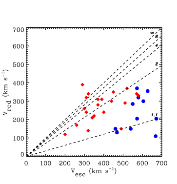
Figure 5.— The maximum red–shifted absorption velocity versus escape velocity for the red–shifted absorption HAEBES in our sample (blue circles) and the CTTSs from FKEH (red diamonds). This plot is a reproduction of Figure 5 from FKEH with the addition of the red–shifted absorption HAEBES from this study. The diagonal dashed lines indicate the maximum infall velocity attained by material originating from the distance (given in units of $R_{*}$) indicated on the right hand side of the plot. The HAEBES on average display maximum absorption velocities that are a smaller percentage of their escape velocities suggesting that material is accreting onto the star from closer to the stellar surface.

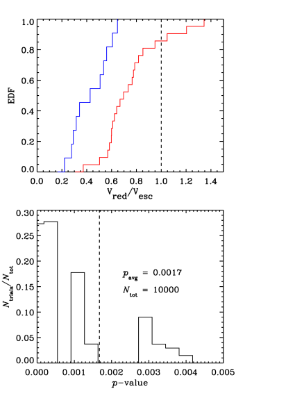
Figure 6.— The emipirical distribution functions (top panel) for the HAEBES (blue line) and CTTSs (red line) from Figure 5 and a histogram of two sample KS test $p$-values (bottom panel) for 10,000 random samplings, limited by an assigned 28% uncertainty in the stellar escape velocity, of the observed velocity ratio distributions. The vast majority of $p$–values are $<$0.01 indicating that the distributions are different at a confidence level $>$99%.

5.2. Outflows and Accretion

5.2.1 Magnetospheric and boundary layer accretion

Magnetospheric accretion appears to be uncommon in mid to early B–type stars but seems to be present at a similar rate to CTTSs in HAe and late HBe stars. Useful information concerning the accretion geometries of the stars in our sample can be gained from narrowing our analysis to only the stars with determined accretion rates. If HAEBES occupy a broad range of evolutionary states, it is certainly possible that many negligibly accreting objects are present in our sample which would lower the occurrence rate of IPC profiles at He I $\lambda$10830, although we have attempted to remove these objects from the sample (see §3.1). EFHK and FKEH show that red–shifted absorption signatures at He I $\lambda$10830 are absent for CTTSs with 1–$\mu$m veilings $>$0.5, with veiling defined as the ratio of the excess emission to the underlying stellar photosphere (see Hartigan et al. 1989). Higher veiling at 1 $\mu$m has been shown to scale with other accretion indicators in CTTSs, indicating that objects with higher accretion rates will show higher veilings (Fischer et al. 2011). FKEH suggests this may be the result of different accretion geometries becoming important in CTTSs with higher accretion rates, i.e. MA may be inhibited by magnetospheres being crushed down to the stellar surface due to high disk accretion rates. Smaller magnetospheres in HAEBES could mimic this result since weaker red–shifted absorption tends to be produced by these geometries compared to larger magnetospheres (FKEH). These weak signatures may be masked by emission in an outflow and further reducing the incidence of red-shifted absorption.

To test this hypothesis in our HAEBE sample, in Figure 7 we have plotted the mass accretion rate (column 7 from Table 2) versus the blue EW minus the red EW. The EW difference is essentially a measure of profile type since negative values imply IPC profiles and positive values imply P–Cygni profiles; objects with centered emission or absorption, or no features, should be near zero. Accretion rates with upper limits are indicated by the downward arrows. The mean accretion rate for our sample (log($\dot{M}$)$\;\buildrel<\over{\sim}\;$-7.1) is indicated by the horizontal dashed line. Figure 7 clearly shows that there is a relative lack of objects with low accretion rates which display P–Cygni profiles. In other words, the objects in our sample with the lowest accretion rates predominantly show red absorption in their He I $\lambda$10830 profiles and the highest accretion rate objects are PC objects. There are also four objects with average accretion rates that show red absorption. Thus, the trend seen in CTTSs for highly accreting stars to not show red–shifted absorption seems to be present in our HAEBE sample. We note that there is no significant statistical difference between the accretion rate distributions of the PC and IPC objects in Figure 7, i.e. a KS test results in a $p$–value of 0.38.

Our spectra are not simultaneous with the observations used to determine the values of $\dot{M}$ and accretion onto young stars is intrinsically variable (Bouvier et al. 2003). Accretion signatures can also be variable due to the combined geometric effects of stellar rotation and magnetic field inclination angle, mimicking real changes in the accretion rate (e.g. Symington et al. 2005; Bouvier et al. 2007a). A more complete data set would combine simultaneous, independent measurements of both $\dot{M}$ and He I $\lambda$10830 EW. Mendigutía et al. (2011) estimate that HAEBE accretion rates in general vary by $\sim$0.5 dex, or a factor of $\sim$3, on timescales of days to months. The He I $\lambda$5876 line, which immediately precedes He I $\lambda$10830 in a recombination–cascade sequence, has a highly variable morphology in some objects (Mendigutía et al. 2011). However, the total He I $\lambda$5876 equivalent width only varies by $\sim$1.5 Åin even the most highly variable objects. Since we might expect changes in He I $\lambda$5876 to reflect similar changes in He I $\lambda$10830, even the largest changes in equivalent width would only impact the 3 red–shifted absorption objects in Figure 7 with equivalent width differences of $<$-1.5. Thus while variability may certainly impact individual objects, we believe the general trend seen in Figure 7 will not be significantly altered. This should be tested with simultaneous determinations of the equivalent width and accretion rate, as mentioned above.

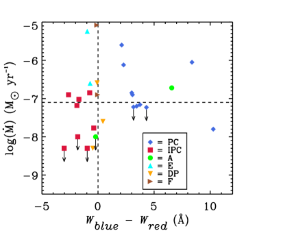
Figure 7.— Blue equivalent widths minus red equivalent widths versus accretion rate for the stars in our sample with measured accretion rates. The profile type abbreviations in the legend are the same as those used in Figure 4 and Table 3. Upper limits on accretion rates are marked with a downward arrow. The horizontal dashed line is the mean accretion rate for the objects in our sample. There is a dearth of stars with P–Cygni–like profiles at low accretion rates and a relative lack of red–shifted absorption objects with large accretion rates.

If red–shifted absorption at He I $\lambda$10830 in CTTSs with large accretion rates tends to be suppressed due to a crushed magnetosphere, then the relative lack of red–shifted absorption in HAEBES with large accretion rates suggests that a similar scenario is operating around these objects. The weaker magnetic field strengths on HAEBES compared to CTTSs supports the idea that large accretion rates are able to force the magnetosphere down to smaller radii, with the extreme cases (e.g. very weak magnetic fields or very large accretion rates) potentially resulting in boundary layer accretion. If the magnetospheres around HAEBES are intrinsically smaller and the field strengths are weaker, then increases in the accretion rate may more easily crush the magnetosphere closer to the stellar surface, resulting in the lower incidence of red–shifted absorption in HAEBES with large accretion rates. Figure 7 also shows a relative lack of blue–shifted absorption at low accretion rates. If HAEBE magnetospheres are crushed by large mass accretion rates, this would indicate that the outflows around HAEBES are predominantly driven by boundary layer–type accretion since the blue–shifted absorption profiles are predominantly produced by objects with large $\dot{M}$. However, as pointed out by FKEH for the CTTSs, the lack of red–shifted absorption could also be due to the filling in of red–shifted absorption by wind emission and not the altering of the accretion geometry. The lack of simultaneous red and blue–shifted absorption in our sample, however, suggests it is the latter since simultaneous accretion and outflows would likely result in observable simultaneous blue and red–shifted absorption in at least some objects.

If many accreting HAEBES have smaller magnetospheres or are accreting through a boundary layer, then the truncation radius will be smaller or nonexistent. The lack of a truncated disk has implications for planet migration down to small orbital radii. It was first suggested by Lin et al. (1996) that planetary migration may eventually be halted by a resonance interaction with the truncated inner–disk. If this mechanism contributes to halting inward planet migration, and sufficiently truncated disks are not present in many HAEBE systems, then the frequency of gas giant planets in close orbits ($r$$<$0.10 AU) should be much lower than for solar–mass objects. We note that simulated density functions by Plavchan & Bilinski (2013) recently found evidence that this migration–halting scenario does not match the orbital distribution of Jupiter–mass planets as well as a tidal circularization model does. However, this analysis was performed for objects with masses $<$1.5 ${\rm\,\it{M_{\odot}}}$ due to the small statistics for planets around F, A, and B–type stars. A larger sample of orbital radii for giant planets around F, A, and B stars will provide a better basis for comparing how the lack of inner disks during early stellar evolution can affect planet migration.

5.2.2 Disk winds

When comparing the He I $\lambda$10830 profiles of our HAEBES to the CTTS profiles in EFHK, a feature that differs significantly between the two samples is that the HAEBE sample shows no evidence of narrow, blue–shifted absorption at any velocity. We exclude the possible case of MWC 137 due to its unknown system RV. According to the models of KEF the key profile signature of a disk wind is narrow blue–shifted absorption resulting from the scattering of stellar photons along streamlines extending outward at some angle from the disk. The small range in absorbed velocities is due to the fact that the line of sight to the stellar surface only intersects a small range of velocities in the disk wind, compared to the entire range of velocities, including the acceleration zone, for wind streamlines that originate on the star. As the inclination of the system becomes more edge–on, the absorption tends to become stronger.

KEF find $\sim$29% of the EFHK CTTS sample to be good disk wind candidates at He I $\lambda$10830; our sample contains no strong disk wind candidates. Outflows launched from near the interaction region of the disk and stellar magnetosphere are a natural consequence of magnetically controlled accretion (e.g. Mohanty & Shu 2008; Kurosawa & Romanova 2012; Zanni & Ferreira 2013). Thus it is expected that some type of disk wind signature would be present in a non–zero fraction of accreting HAEBE profiles if MA involving large magnetospheres were the dominant accretion mechanism. On the other hand, if HAEBES tend to have smaller magnetospheres than CTTSs, a disk–wind launched from a range of radii near the truncation point closer to the stellar surface would become indistinguishable from a stellar wind for most viewing angles. This is especially true for X–wind configurations where the wind launching region is confined to a very narrow annulus near the corotation radius (Shu et al. 1994). Thus we cannot rule out the presence of disk winds in our sample based on the lack of narrow blue–shifted absorption profiles. We note that the lack of direct inner disk wind evidence in our sample does not conflict with the recent interpretations of interferometric observations of Br$\gamma$ in a small number of HAEBES as arising in a disk wind (Tatulli et al. 2007; Kraus et al. 2008). The disk winds diagnosed in these cases (specifically DX Cha, HD 163296, and V921 Sco Kraus et al. 2008) likely arise over much larger radii (i.e. near the dust sublimation radius at a few tenths of an AU) than are traced by He I $\lambda$10830.

5.2.3 Accretion–driven outflows in the IPC objects

There is an important difference between the IPC profiles in our HAEBE sample and the CTTSs from EFHK: blue–shifted absorption, indicating a disk or stellar wind, is present in 16 of 21 CTTSs that also show red–shifted absorption. The 13 stars with red–shifted absorption or IPC profiles in our sample do not show any evidence of blue–shifted wind signatures. There is a strong correlation between accretion and outflow rates in TTSs (e.g. Hartigan et al. 1995) which points to mass accretion being the main driver of outflows in these objects. The presence of outflow signatures in CTTS He I $\lambda$10830 IPC profiles also supports this conclusion. The relationship between mass accretion and mass outflow extends into the HAEBE mass range (e.g. Ellerbroek et al. 2013). Since this relationship seems to apply to HAEBES, we would expect to see some sort of outflow signature at He I $\lambda$10830 in a fraction of the IPC objects. Since this is not observed, and since literature H$\alpha$ profiles (e.g. Finkenzeller & Mundt 1984; Hamann & Persson 1992; Mendigutía et al. 2011) of the IPC objects do not show any direct evidence of blue–shifted wind signatures, it is currently unclear whether or not mass accretion is capable of driving strong outflows on these objects. As noted in §5.2.1 the IPC objects generally have average or below–average accretion rates. Based on the $\dot{M}_{W}$ vs $\dot{M}_{acc}$ relationship from Ellerbroek et al. (2013), accretion rates of this magnitude should be able to drive detectable outflows. Similar average accretion rates ($\sim$10^-7 ${\rm\,\it{M_{\odot}}}$ yr^-1) are seen in some of the PC objects confirming that these accretion rates are capable of driving outflows. This suggests that the IPC objects, which show evidence of MA, are less efficient at driving outflows compared to the PC objects which may be accreting through a different mechanism (see §5.2.4).

The presence of red–shifted absorption at He I $\lambda$10830 requires the existence of infalling material near the star. The lack of outflow signatures in our IPC objects suggests that these stars do not have strong accretion–powered outflows. It is unlikely that this is due to differing formation conditions for the wind versus the accretion flow since He I $\lambda$10830 signatures tracing outflowing gas is expected to form at similar distances from the star as the accreting material. In addition, the relative lack of strong outflows in HAEBES as a whole is supported by optical forbidden line statistics which show a much lower fraction of occurrence of large scale outflows in HAEBES than in CTTS (e.g. Hamann & Persson 1992). If HAEBE magnetospheres are smaller than those of CTTSs, it may be more difficult to produce the magnetic configurations at the disk–magnetosphere interaction region necessary to drive strong outflows. Furthermore, mass infall from deeper in the star’s gravitational potential will result in less of the necessary energy to accelerate an outflow from the stellar surface. Thus accretion driven stellar winds in HAEBES experiencing MA may be less efficient. To our knowledge, no simulations of the magnetospheric star–disk interaction region have been performed using typical HAEBE parameters. MHD calculations using HAEBE parameters would be informative.

5.2.4 Accretion–driven outflows in the PC objects

None of the P–Cygni objects in our sample show evidence of mass infall in He I $\lambda$10830. FKEH showed that weak red–shifted absorption is produced at most inclinations angles for stars with low veilings and truncation radii of $\sim$2 $R_{*}$. These weak absorption signatures could be overwhelmed by strong emission in a wind (Kwan et al. 2007). Red–shifted absorption from a MA flow would also be absent for inclination angles near $\sim$0^∘. Thus it is possible to see evidence of an accretion–launched outflow without seeing any direct signature of mass infall. However, the significant lack of red–shifted absorption seen in HBe He I $\lambda$10830 profiles compared to HAe stars and CTTSs suggests mass infall is truly absent rather than being the result of viewing angle effects or filling in by wind emission. An alternative to MA is to drive the outflows from an equatorial boundary layer created by the accretion disk at the stellar surface. This will be discussed below in §5.4. We note that only one object in our sample has an estimated luminosity high enough (MWC 1080; $L_{*}$$\sim$3.8 x 10⁴ ${\rm\,\it{L_{\odot}}}$) to potentially produce a radiatively driven wind of any significance (Krtička 2014). Thus the strong outflows observed in our sample are most likely accretion related.

5.3. Herbig Ae vs Be stars

There is growing consensus that Herbig Ae (HAe) stars interact with their environments differently than Herbig Be (HBe) stars. In particular, HBe objects are found to show weaker evidence for MA, including line widths inconsistent with gas rotating at Keplerian velocities near or inside of the disk truncation radius (Mendigutía et al. 2011), a lower incidence of line polarization effects due to scattering of stellar photons by disk–like circumstellar material (Vink et al. 2002; Mottram et al. 2007), differences in excitation conditions of H₂ (Martin–Zaïdi et al. 2008), and a possible breakdown of the Br $\gamma$–accretion luminosity relationship that holds for CTTSs and HAe stars (Donehew & Brittain 2011), although we note that the accretion luminosities determined by Donehew & Brittain (2011) are calculated with a relationship derived using an A2V photosphere which may under–predict $L_{acc}$ for stars with spectral types earlier than A2. A preliminary analysis of He I $\lambda$10830 data presented by Oudmaijer et al. (2011) for 79 HAEBES shows a shift from absorption dominated profiles in HAe objects to more emission dominated profiles in HBe objects (Figure 3 from Oudmaijer et al. 2011). We note that our data do not display this trend: we find no relationship between the total He I $\lambda$10830 EW and effective temperature. The observed differences between HBe and HAe objects may indicate that, in general, the two groups are being observed at different phases of their pre–main sequence evolution. More specific evolutionary classifications, as proposed, for example, by Malfait et al. (1998), would facilitate comparisons between objects that are at more similar stages of development. A second, although related, possible source of the observed differences is the misclassification of classical Be objects as HBe stars (see §4.1). It is unlikely that the PC and IPC HBe stars in our sample are misclassified since their H$\alpha$ features, in general, do not match the typical zero–velocity centered double–peaked emission of the classical Be objects (Hanuschik 1996).

Assuming that all of the objects in our sample not discussed in §4.1 are actually HAEBES, the HBe stars show different rates of occurrence of particular line profile morphologies compared to the HAe stars (Table 4), although the contingency tests result in relatively high $p$–values (Table 6) indicating that the red and blue–shifted absorption incidence is not significantly different between the two groups. The statistics are illustrated in Figure 8 where it is shown that any significant red–shifted absorption is almost completely absent from the HBe sample (symbols above the horizontal dotted line). There is only one early B–type object (HD 200775, a B4 star) that displays a red–shifted absorption profile. Note that MWC 137 is included in the figure (right– most left–facing purple triangle), although it is excluded from the statistics in Table 4 due to the lack of a reliable RV estimate. The HAe stars show a diverse variety of both PC and IPC profiles, indicating greater overall levels of accretion and outflow activity.

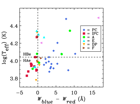
Figure 8.— Effective temperature versus blue minus red He I $\lambda$10830 equivalent width. Plotting symbols and colors are the same as in Fig. 7 with the exception of V374 Cep and MWC 137 which are plotted as a left–pointing purple triangles. An approximate separation between A and B spectral types is marked by the horizontal dotted line. Potentially misclassified objects from §3.1 are excluded. Note the lack of B–type stars in the upper left quadrant.

Although the differences in line profile morphology are not statistically significant for our sample, Figure 8 provides a hint that physical differences do exist between the HAe and HBe environments. Thus we argue that our data add to the recent evidence suggesting that there is a distinction between HAe and HBe stars concerning the circumstellar environment within a few stellar radii of the star. The late B–type objects are likely more similar to HAe stars than to early B–type objects. The greater incidence of IPC profiles in HAe stars suggests that mass accretion in a substantial fraction of these objects is occurring along magnetic field lines. HBe objects show a much lower incidence of IPC morphologies, although the sample size is small. Outflows seem to be present in similar numbers in both populations. The observed differences in the line profile statistics could be due to differing physical conditions in the immediate circumstellar environments of HAe and HBe stars. On the other hand, if the conditions around both groups of objects are similar, our data would indicate that accretion in HBe objects, and potentially some HAe stars, is occurring through a different mechanism, e.g. a boundary layer at the stellar surface. This was been previously suggested by Mendigutía et al. (2011). Boundary layer accretion would naturally explain the relative lack of red–shifted absorption features in HBe stars. The questions concerning the physical conditions in the immediate circumstellar environment can be further addressed with a larger sample size using optical and UV data. We are currently pursuing this (Cauley & Johns–Krull 2014, in prep).

5.4. Outflows driven from the boundary layer

If boundary layer accretion is partially responsible for the lack of red–shifted absorption signatures in HBe stars, and possibly for the smaller observed incidence in HAe stars compared to CTTSs, a natural question arises: can boundary layer accretion drive outflows in the same way as MA since outflows are seen in an appreciable fraction of both HAe and HBe stars? The luminosity released by the boundary layer differs from the luminosity of a magnetically channeled funnel flow by a negligible factor, at least for reasonable stellar parameters. Thus the energy required to drive outflows from near or at the stellar surface is readily available in the boundary layer paradigm. In current 3D MHD models of accretion–generated outflows around TTSs, magnetic fields provide the main acceleration mechanism and geometric constraint for the expanding wind (e.g. Romanova et al. 2005, 2009). As we have pointed out, there is currently no observational support for the existence of magnetic fields on the majority of HAEBES which are required to drive and support these flows. However, it has also been suggested that accretion–powered stellar winds are driven by a combination of thermal and centrifugal effects, the thermal effects being driven by the accretion–heated stellar corona (Matt & Pudritz 2005). Alfvén waves excited by accreting material may also play a role in driving the wind, although this mechanism also requires a magnetic field.

X–ray observations have shown a fraction ($\sim$50%) of HAEBES to be x–ray emitters, although this is an upper limit since it is unclear if the x–ray emission is intrinsic to the HAEBES or from unresolved low–mass companions (Stelzer et al. 2006, 2009). The small detected HAEBE x–ray–to–bolometric luminosity ratios (log($L_{x}$/$L_{bol}$)$\sim$-6.3; Stelzer et al. 2009) and the moderate fraction of x–ray emitters detected suggests that most HAEBES do not have sufficiently active coronae to drive strong Alfvén waves or thermal winds. It is unclear what effect the deposition of energy near the stellar equator will have compared to the higher latitudes that are characteristic of magnetically channeled accretion. However, one possible scenario is the X–celerator mechanism proposed by Shu et al. (1988) in which a wind is driven from a boundary layer at the interface between a star rotating near break–up velocity and an accretion disk. Many HAEBES have measured vsini values that are significant fractions of their break–up velocities. These boundary layer outflows, however, also require a magnetic field at the interaction region, although the required field strengths are small enough ($\sim$10–20 G for typical HAEBE parameters; Shu et al. (1988)) to be within the current observational uncertainties for many objects (Alecian et al. 2013). The high detection rate of PC profiles for accreting stars in our sample indicates that stellar winds are common among accreting HAEBES. Although our data are not conclusive, the indication that the PC objects are not accreting magnetically lends itself to the boundary layer accretion–driven stellar wind scenario. These winds are likely generated partially by the high rotation rates of HAEBES. Thus we tentatively conclude that boundary layer accretion in HAEBES, assisted by centrifgual acceleration, is able to drive strong stellar winds.

5.5. HAEBES as massive CTTSs?

HAEBES are often identified as the higher mass analogues of CTTSs (e.g. Muzerolle et al. 2004; Skinner et al. 2004; Grady et al. 2010). In reality, line profile statistics, including those gathered here, point to significant differences between the incidence, and likely the physical nature, of the mass flows in HAEBES compared to CTTSs. The optical permitted line study of CTTSs performed by Alencar & Basri (2000) found very high rates of outflow and accretion indicators, 80% and 40% respectively, in a sample of 30 CTTSs. A smaller sample of 15 objects was presented by Edwards et al. (1994) with an even larger incidence (87%, or 13 of 15 objects) of red–shifted absorption in at least one line diagnostic. A large sample of HAEBES studied by Finkenzeller & Mundt (1984) found only a 29% incidence of blue–shifted absorption and only a 3% incidence of red–shifted absorption at H$\alpha$ or Na I. Blue–shifted forbidden line emission with both high and low–velocity components is detected in almost all CTTSs (e.g. Hartigan et al. 1995), indicating the presence of extended collimated outflows. Similar line profiles are detected at a much lower rate in HAEBES: Corcoran & Ray (1997) found only 15% of their 56 HAEBES display this characteristic while Böhm & Catala (1994) find evidence of blue–shifted forbidden line emission in only 3%of their sample.

Our sample continues the trend of disparate line morphology statistics between HAEBES and CTTSs. In particular, outflows in both HAe and HBe stars seem to be much less common than in CTTSs while MA signatures are present in a similar but slightly lower rate in HAe stars compared to CTTSs. HBe stars show a considerably lower rate of red–shifted absorption signatures. These conclusions are confirmed by the contingency test $p$–values given in Table 6. The tests provide strong evidence that the rates of occurrence of these mass flow signatures differ between the two mass regimes and perhaps between HAe and HBe stars, although the statistical evidence is weaker for the differences between the HAEBE subgroups. Based on the He I $\lambda$10830 data then, it appears that the immediate circumstellar environments of HAEBES and CTTSs cannot be treated identically as a general rule.

The differences in He I $\lambda$10830 morphology statistics between HAEBES and CTTSs may be caused in part by smaller magnetospheres mediating the star–disk interaction in HAe and some HBe stars, as suggested by the results in §5.1.2. In addition, this would lead to a lower incidence of red–shifted absorption signatures in HAEBES, which is observed, due to fewer viewing angles that intersect the infalling part of the flow. The differing statistics may also be a result of the varying stages of pre–main sequence evolution included in our sample: we simply may not be comparing objects at similar enough stages of evolution, although we have attempted to remove the most obvious imposters from our sample. More precise evolutionary subclasses for HAEBES, similar to those for WTTSs and CTTSs, may account for the differences in line statistics observed here.

As outlined in §2, smaller magnetospheres should result in smaller values of $R_{A}$. The ratio $R_{A}$/$R_{*}$ is shown in Figure 9 for the CTTSs (red asterisks) exhibiting blue–shifted absorption from EFHK and for the HAEBES (blue circles and green triangles) from this study showing blue–shifted absorption. The green triangles are V380 Ori and HD 190073 which are both slowly rotating magnetic HAEBES. The right–hand axis shows the corotation radius. On average, the HAEBES have smaller values of $R_{A}$, and thus smaller corotation radii, than the CTTSs. This is mainly driven by the high $v$sin$i$ values of the HAEBES but this supports the idea that strong outflows can be launched from closer to the star and is consistent with the idea of smaller magnetospheres on HAEBES. The Shu et al. (1988) X–celerator mechanism is, in fact, the limiting case of a magnetosphere being pushed to the stellar surface with the outflow being launched centrifugally along some of the open field lines. Thus it is not surprising that we see outflows in HAEBES that are potentially launched from a point relatively closer to the stellar surface than seen in CTTSs.

Figure 9.— Alfvén radius, $R_{A}$, plotted against $T_{eff}$ for the blue–shifted absorption CTTSs from EFHK (red asterisks) and the blue–shifted absorption HAEBES from this study (blue circles and green triangles). The corotation radius, $R_{co}$, corresponding to each $R_{A}$ is shown on the right–hand axis. The green triangles are V380 Ori and HD 190073, both confirmed slowly rotating magnetic HAEBES. The HAEBES, in general, show smaller values of $R_{A}$ and $R_{co}$ which is consistent with the idea of smaller magnetospheres in HAEBES.

6. SUMMARY AND FUTURE WORK

We have presented high resolution He I $\lambda$10830 observations of a large sample of Herbig Ae/Be stars. These objects display a wide variety of line profile morphologies, including classical P–Cygni and inverse P–Cygni profiles. Our results are summarized as follows:

• A number of objects in our sample (7 of 56) do not display line profiles characteristic of young stars interacting with their environments. These stars are flagged as having been potentially misidentified as HAEBES.

• We find that there appear to be differences between the He I $\lambda$10830 line profile properties of HBe stars compared to HAe stars. In particular, HBe objects tend to display blue absorption with little evidence for infalling material; the HAe sample shows both blue and red shifted absorption features indicating overall higher levels of mass flow activity. This may indicate that HBe objects do not experience accretion in the same manner as HAe stars, i.e. instead of accreting along magnetic field lines from a disk, accretion occurs through a boundary layer at the surface of the star.

• HAe stars show a similar incidence of He I $\lambda$10830 red–shifted absorption to CTTSs while the incidence in HBe stars is significantly lower. Both HAe and HBe stars show a much lower incidence of blue–shifted absorption than is found in CTTSs. This suggests that HAe and especially HBe environments cannot be treated as the intermediate mass analogs of CTTS systems.

• In objects that display red–shifted absorption, we observe no simultaneous blue–shifted absorption, a feature common to CTTSs. Some blue absorption is expected (for most viewing angles) due to winds that are launched from the inner disk or stellar surface. Since none of the objects in our sample with clear red–shifted absorption show signs of blue absorption, it is unclear whether or not these objects are capable of launching accretion–generated outflows.

• The red–shifted absorption profiles in our sample show maximum absorption velocities that are smaller percentages of the system escape velocity than is found in CTTSs, suggesting these mass inflows originate closer to the star. This may be a result of more compact magnetospheres in HAEBES resulting in smaller disk truncation radii. This is expected for the magnetospheric accretion scenario for HAEBES due to their high rotation rates and weak or nonexistent magnetic fields.

• None of the objects in our sample show any sign of narrow blue–shifted absorption indicative of pure disk winds, which are common at He I $\lambda$10830 in CTTSs. We interpret these results as evidence that the inner environments around HAEBES cannot be considered scaled analogues of CTTS environments. More specifically, the magnetocentrifugally driven winds that are, theoretically, launched from near the interaction region of the stellar magnetosphere and accretion disk in CTTSs are not clearly indicated in HAEBES or are too weak to be detected in our data. This is supported by the lack of detected magnetic fields on HAEBES. Instead, stellar winds seem to be the only outflow mechanism for the objects in our sample. However, magnetocentrifugally driven ouflows from the star–disk interaction region can appear as stellar winds if the interaction region is near enough to the star. Thus these outflows cannot be ruled out based on the data presented here. We find that for HAEBES that do show outflow signatures, these can be driven from smaller magnetospheres than required for CTTSs. Finally, since stellar magnetic fields are either absent or too weak to be detected around most HAEBES, and since we detect no disk wind signatures in our sample, we suggest that the magnetic fields involved in launching disk winds in CTTSs are stellar in origin and not disk–generated or primordial. This would naturally explain the lack of obvious disk winds in HAEBES and their common appearance in CTTS systems.

One potential cause for the differences between profile statistics in HAe and HBe stars and between HAEBES and CTTSs is the likely spread of evolutionary stages present in the current catalog of HAEBES. The more rapid evolution of HAEBES, and especially HBe stars, compared to CTTSs results in a smaller chance of observing a particular HAEBE at any stage of its contraction towards the main sequence. Thus it would be more informative to only compare HAe and HBe stars at the same stages of evolution and to only compare CTTSs with HAEBES that are in the HAEBE equivalent of the CTTS phase. Malfait et al. (1998) suggested an evolutionary classification for HAEBES based on IR colors similar to the groupings given by Hillenbrand et al. (1992). The relevant CTTS phase in the Malfait et al. (1998) scheme would be panels (b) and (c) of their figure 3. A comparison of objects within these sub–groups may be more precise than the analysis presented here. However, a larger sample size than the one presented in this work would be needed to make such a comparison meaningful.

As suggested by EFHK, and numerically studied by Kwan & Fischer (2011), simultaneous measurements of He I $\lambda$5876 and He I $\lambda$10830 would provide constraints on the physical conditions of He I $\lambda$10830 line formation. Data sets of this type, to our knowledge, have not been published. Similar sample sizes of these data for CTTSs and HAEBES would facilitate an excellent comparison between the wind launching and accretion regions for the two groups and help clarify the origin of the statistical differences of line profile type presented in this work. We are presently pursuing this for a small sample of HAEBES.

The lack of observed wind signatures in the IPC objects in our sample is puzzling considering the high rate (76% from EFHK) of CTTSs showing both red–shifted absorption and blue-shifted absorption. We are currently analyzing a large sample of optical and UV HAEBE data. The analysis presented here will be extended in these studies with the hope of shedding light on this significant difference between HAEBES and CTTSs. In addition, variability studies of He I $\lambda$10830 in HAEBES will help clarify whether simultaneous red and blue–shifted absorption is truly absent or if our current data set is anomalous.

References

- Acke & van den Ancker (2004) Acke, B., & van den Ancker, M. E. 2004, A&A, 426, 151
- Alecian et al. (2013) Alecian, E., et al. 2013, MNRAS, 429, 1001
- Alencar & Basri (2000) Alencar, S. H. P., & Basri, G. 2000, AJ, 119, 1881
- Alonso–Albi et al. (2009) Alonso–Albi, T., et al. 2009, A&A, 117, 136
- Appenzeller et al. (1984) Appenzeller, I., Jankovics, I., & Östreicher, R. 1984, A&A, 151, 108
- Basri & Batalha (1990) Basri, G., & Batalha, C. 1990, ApJ, 363, 654
- Bertout et al. (1988) Bertout, C., Basri, G., & Bouvier, J. 1988, ApJ, 330, 350
- Blondel & Tjin A Djie (2006) Blondel, P. F. C., & Tjin A Djie, H. R. E. 2006, A&A, 456, 1045
- Böhm & Catala (1994) Böhm, T., & Catala, C. 1994, A&A, 290, 167
- Böhm & Catala (1995) Böhm, T., & Catala, C. 1995, A&A, 301, 155
- Bossier et al. (2011) Bossier, J., et al. 2011, A&A, 531, A50
- Bouvier et al. (2003) Bouvier, J., et al. 2003, A&A, 409, 169
- Bouvier et al. (2007) Bouvier, J., Alencar, S. H. P., Harries, T. J., Johns–Krull, C. M., and Romanova, M. M. 2007, Protostars and Planets V, eds. B. Reipurth, D. Jewitt, K. Keil, University of Arizona Press, Tucson, 951 pp., 2007, 479
- Bouvier et al. (2007a) Bouvier, J., et al. 2007, A&A, 463, 1017
- Calvet & Hartmann (1992) Calvet, N., & Hartmann, L. 1992, ApJ, 386, 239
- Calvet & Gullbring (1998) Calvet, N., & Gullbring, E. 1998, ApJ, 509, 802
- Cameron & Campbell (1993) Cameron, A. C., & Campbell, C. G. 1993, A&A, 274, 309
- Carmona et al. (2010) Carmona, A., van den Ancker, M. E., Audard, M., Henning, Th., Setiawan, J., & Rodmann, J. 2010, A&A, 517, A67
- Chen et al. (2012) Chen, L., et al. 2012, A&A, 541, A104
- Corcoran & Ray (1997) Corcoran, M., & Ray, T. P. 1997, A&A, 321, 189
- Corporon & Lagrange (1999) Corporon, P., & Lagrange, A.–M. 1999, A&ASS, 136, 429
- Dent et al. (2005) Dent, W. R. F., Greaves, J. S., & Coulson, I. M. 2005, MNRAS, 359, 663
- Donehew & Brittain (2011) Donehew, B., & Brittain, S. 2011, AJ, 141, 46
- Donati et al. (2010) Donati, J.–F., et al. 2010, MNRAS, 409, 1347
- Donati et al. (2011) Donati, J.–F., et al. 2011, MNRAS, 417, 1747
- Donati et al. (2011a) Donati, J.–F., et al. 2011, MNRAS, 412, 2454
- Dupree et al. (2005) Dupree, A. K., Brickhouse, N. S., Smith, G. H., & Strader, J. 2005, ApJ, 625, L131
- Edwards et al. (1987) Edwards, S., Cabrit, S., Strom, S. E., Heyer, I., Strom, K. M., & Anderson, E. 1987, ApJ, 321, 473
- Edwards et al. (1994) Edwards, S., Hartigan, P., Ghandour, L., & Andrulis, C. 1994, AJ, 103, 3
- Edwards et al. (2006) Edwards, S., Fischer, W., Hillenbrand, L., & Kwan, J. 2006, ApJ, 646, 319
- Eisner et al. (2004) Eisner, J. A., Lane, B. F., Hillenbrand, L. A., Akeson, R. L., & Sargent, A. I. 2004, ApJ, 613, 1049
- Eisner et al. (2007) Eisner, J. A., Chiang, E. I., Lane, B. F, & Akeson, R. L. 2007, ApJ, 657, 347
- Eisner et al. (2009) Eisner, J. A., Graham, J. R., Akeson, R. L., & Najita, J. 2009, ApJ, 692, 309
- Elias et al. (2006) Elias, J. H., Joyce R. R., Liang, M., Muller, G. P., Hileman, E. A., & George, J. R., 2006, in McLean I. S., Iye M., eds, Proc. SPIE Conf. Ser. Vol. 6269, Ground–based and Airborne Instrumentation for Astronomy. SPIE, Bellingham, p. 62694C
- Ellerbroek et al. (2013) Ellerbroek, L. E., et al. 2013, A&A, 551, A5
- Feigelson & Babu (2012) Feigelson, E. D., & Babu, G. J. 2012, Modern Statistical Methods for Astronomy (New York, NY: CUP)
- Finkenzeller & Mundt (1984) Finkenzeller, U., & Mundt, R. 1984, A&ASS, 55, 109
- Finkenzeller (1985) Finkenzeller, U. 1985, A&A, 151,340
- Fischer et al. (2008) Fischer, W., Kwan, J., Edwards, S., & Hillenbrand, L. 2008, ApJ, 687, 1117
- Fischer et al. (2011) Fischer, W., Edwards, S., Hillenbrand, L., & Kwan, J. 2011, ApJ, 730, 73
- Fuente et al. (2002) Fuente, A., Martín–Pintado, J., Bachiller, R., Rodríguez–Franco, & Palla, F. 2002, A&A, 387, 977
- Fukagawa et al. (2003) Fukagawa, M., Tamura, M., Itoh, Y., Hayashi, S. S., & Oasa, Y. 2003, ApJ, 590, L49
- Garcia Lopez et al. (2006) Garcia Lopez, R., Natta, A., Testi, L., & Habart, E. 2006, A&A, 459,837
- Garrison (1978) Garrison, Jr., L. M. 1978, ApJ, 224, 535
- Ghandour et al. (1994) Ghandour, L., Strom, S., Edwards, S., & Hillenbrand, L. 1994, The First Conference on the Nature and Evolutionary Status of Herbig Ae/Be stars, A. S. P. Conf. Ser., Vol. 62, 223
- Grady et al. (2000) Grady, C. A., et al. 2000, ApJ, 544, 895
- Grady et al. (2010) Grady, C. A., et al. 2010, ApJ, 719, 1565
- Guilloteau et al. (2011) Guilloteau, S., Dutrey, A., Piétu, V., & Boehler, Y. 2011, A&A, 529, A105
- Guilloteau et al. (2013) Guilloteau, S., Di Folco, E., Dutrey, A., Simon, M., Grosso, N., & Piétu, V. 2013, A&A, 549, A92
- Guimarães et al. (2006) Guimarães, M. M., Alencar, S. H. P., Corradi, W. J. B., & Vieira, S. L. A. 2006, A&A, 457, 581
- Groh et al. (2007) Groh, J. H., Damineli, A., & Jablonski, F. 2007, A&A, 465, 993
- Hamann & Persson (1992) Hamann, F., & Persson, S. E. 1992, ApJSS, 82, 285
- Hamann (1994) Hamann, F. 1994, ApJSS, 93, 485
- Hanuschik (1996) Hanuschik, R. W. 1996, A&A, 308, 170
- Hartigan et al. (1989) Hartigan, P., Hartmann, L., Kenyon, S., Hewett, R., & Stauffer, J. 1989, ApJSS, 70,899
- Hartigan et al. (1991) Hartigan, P., et al. 1991, ApJ, 382, 617
- Hartigan et al. (1995) Hartigan, P., Edwards, S., & Ghandour, L. ApJ, 452, 736
- Hartmann et al. (1993) Hartmann, L., Kenyon, S. J., & Calvet, N. 1993, ApJ, 407, 219
- Hartmann et al. (1994) Hartmann, L., Hewett, R., & Calvet, N. 1994, ApJ, 426, 669
- Herbig (1960) Herbig, G. H. 1960, ApJS, 4, 337
- Hernández et al. (2004) Hernández, J., Calvet, N., Briceo, C., Hartmann, L., & Berlind, P. 2004, ApJ, 127, 1682
- Hillenbrand et al. (1992) Hillenbrand, L. A., Strom, S. E., Vrba, F. J., & Keene, J. 1992, ApJ, 397, 613
- Hinkle et al. (1998) Hinkle, K. H., et al. 1998, Proc. SPIE, 3354, 810
- Hinkle et al. (2001) Hinkle, K. H., Joyce, R. R., Hedden, A., Wallace, L., & Engleman Jr., R. 2001, PASP, 113, 783, 548
- Hinkley et al. (2013) Hinkley, S., et al. 2013, ApJL, 763, L9
- Howarth & Schmutz (1992) Howarth, I. D., & Schmutz, W. 1992, A&A, 261, 503
- Iben (1967) Iben, I., Jr. 1967, ARA&A, 5,571
- Johns–Krull (2007) Johns–Krull, C. M. 2007, ApJ, 664, 975
- Königl (1991) Königl, A. 1991, ApJ, 370, L39
- Kraus et al. (2008) Kraus, S., et al. 2008, A&A, 489, 1157
- Kraus et al. (2010) Kraus, S., et al. 2010, Nature, 466, 339
- Krtička (2014) Krtička, J. 2014, A&A, 564, A70
- Kurosawa & Romanova (2012) Kurosawa, R., & Romanova, M. M. 2012, MNRAS, 426, 2901
- Kwan et al. (2007) Kwan, J., Edwards, S., & Fischer, W. 2007, ApJ, 657, 897
- Kwan & Fischer (2011) Kwan, J., & Fischer, W. 2011, 411, 2383
- Lada & Adams (1992) Lada, C. J., & Adams, F. C. 1992, ApJ, 393,278
- Leitner et al. (2004) Leitner, Ch., et al. 2004, A&A, 423, 537
- Lin et al. (1996) Lin, D. N. C., Bodenheimer, P., & Richardson, D. C. 1996, Nature, 380, 606
- Liu et al. (2007) Liu, W. M., et al. 2007, ApJ, 658, 1164
- Malfait et al. (1998) Malfait, K., Bogaert, E., & Waelkens, C. 1998, A&A, 331, 211
- Mannings & Sargent (1997) Mannings, V., & Sargent, A. I. 1997, ApJ, 490, 792
- Mannings et al. (1997) Mannings, V., Koerner, D. W., & Sargent, A. I. 1997, Nature, 388, 555
- Mariñas et al. (2011) Mariñas, N., Telesco, C. M., Fisher, R. S., & Packham, C., 2011, ApJ, 737, 57
- Martin–Zaïdi et al. (2008) Martin–Zaïdi, C., Deleuil, M., Le Bourlot, J., et al. 2008, A&A, 484, 225
- Matt & Pudritz (2005) Matt, S., & Pudritz, R. E. 2005, ApJ, 632, L135
- Matter et al. (2014) Matter, A., et al. 2014, A&A, 561 A26
- Meeus et al. (2001) Meeus, G., Waters, L. B. F. M., Bouwman, J., van den Ancker, M. E., Waelkens, C., & Malfait, K. 2001, A&A, 365, 476
- Mendigutía et al. (2011) Mendigutía, I., et al. 2011, A&A, 529, A34
- Mendigutía et al. (2011) Mendigutía, I., et al. 2011, A&A, 535, A99
- Mendigutía et al. (2012) Mendigutía, I., et al. 2012, A&A, 543, A59
- Millan–Gabet et al. (2001) Millan–Gabet, R., Schloerb, F. P., & Traub, W. A. 2001, ApJ, 546, 358
- Mohanty & Shu (2008) Mohanty, S., & Shu, F. H. 2008, ApJ, 687, 1323
- Mottram et al. (2007) Mottram, J. C., Vink, J. S., Oudmaijer, R. D., & Patel, M. 2007, MNRAS, 377, 1363
- Muzerolle et al. (1998) Muzerolle, J., Calvet, N., & Hartmann, L. 1998, ApJ, 492, 743
- Muzerolle et al. (2001) Muzerolle, J., Calvet, N., & Hartmann, L. 2001, ApJ, 550, 944
- Muzerolle et al. (2004) Muzerolle, J., D’Alessio, P., Calvet, N., & Hartmann, L. 2004, ApJ, 617
- Natta et al. (2001) Natta, A., Prusti, T., Neri, R., Wooden, D., Grinin, V. P., & Mannings, V. 2001, A&A, 371, 186
- Natta et al. (2004) Natta, A., Testi, L., Neri, R., Shepherd, D. S., & Wilner, D. J. 2004, A&A, 416, 179
- Okamoto et al. (2009) Okamoto, Y. K., et al. 2009, ApJ, 706, 665
- Oudmaijer et al. (1992) Oudmaijer, R. D., van der Veen, W. E. C. J., Waters, L. B. F. M., Trams, N. R., Waelkens, C., & Engelsman, E. 1992, A&ASS, 96, 625
- Oudmaijer et al. (2011) Oudmaijer, R. D., et al. 2011, AN, 332, 3, 238
- Palla & Stahler (1991) Palla, F., & Stahler, S. W. 1991, ApJ, 375, 288
- Perrin et al. (2006) Perrin, M. D., Duchne, G., Kalas, P., & Graham, J. R. 2006, ApJ, 645, 1272
- Piskunov et al. (1995) Piskunov, N. E., Kupka, F., Ryabchikova, T. A., Weiss, W. W., & Jeffery, C. S. 1995, A&AS, 112, 525
- Piskunov (1999) Piskunov, N. 1999, Polarization, 243, 515
- Plavchan & Bilinski (2013) Plavchan, P., & Bilinski, C. 2013, ApJ, 769, 86
- Pogodin et al. (2006) Pogodin, M. A., Malanushenko, V. P., Kozlova, O. V., Tarasova, T. N., & Franco, G. A. P. 2006, A&A, 452, 551
- Ragland et al. (2012) Ragland, S., et al. 2012, ApJ, 746, 126
- Romanova et al. (2005) Romanova, M. M., Ustyugova, G. V., Koldoba, A. V., & Lovelace, R. V. E. 2005, ApJ, 635, L165
- Romanova et al. (2009) Romanova, M. M., Ustyugova, G. V., Koldoba, A. V., & Lovelace, R. V. E. 2009, MNRAS, 399, 1802
- Schegerer et al. (2013) Schegerer, A. A., Ratzka, T., Schuller, P. A., Wolf, S., Mosoni, L., & Leinert, Ch. 2013, A&A, 555, A103
- Schütz et al. (2005) Schtz, O., Meeus, G., & Sterzik, M. F. 2005, A&A, 431, 165
- Shu et al. (1988) Shu, F. H., Lizano, S., Ruden, S. P., & Najita, J. 1988, ApJ, 328, L19
- Shu et al. (1994) Shu, F., et al. 1994, ApJ, 429, 781
- Skinner et al. (2004) Skinner, S. L., Güdel, M., Audard, M., & Smith, K. 2004, ApJ, 614, 221
- Stelzer et al. (2006) Stelzer, B., Micela, G., Hamaguchi, K., & Schmitt, J. H. M. M. 2006, A&A, 457, 223
- Stelzer et al. (2009) Stelzer, B., Robrade, J., Schmitt, J. H. M. M., & Bouvier, J. 2009, A&A, 493, 1109
- Strom et al. (1972) Strom, S. E., Strom, K. M., Yost, J., Carrasco, L., & Grasdalen, G. 1972, ApJ, 173, 353
- Symington et al. (2005) Symington, N. H., Harries, T. J., & Kurosawa, R. 2005, MNRAS, 356, 1489
- Tang et al. (2012) Tang, Y.-W., Guilloteau, S., Piétu, V., Dutrey, A., Ohashi, N., & Ho, P. T. P. 2012, A&A, 547, A84
- Tatulli et al. (2007) Tatulli, E., et al. 2007, A&A, 464, 55
- Thé, de Winter, & Pérez (1994) Thé, P. S., de Winter, D., & Péerez, M. R. 1994, A&ASS, 104,315
- Thi et al. (2014) Thi, W.–F., et al. 2014, A&A, 561, A50
- van Boekel et al. (2005) van Boekel, et al. 2005, A&A, 437, 189
- van den Ancker et al. (1997) van den Ancker, M. E., et al. 1997, A&A, 324, L33
- van den Ancker et al. (1998) van den Ancker, M. E., de Winter, D., & Tjin A Djie, H. R. E. 1998, A&A, 330, 145
- Verhoeff et al. (2012) Verhoeff, A. P., et al. 2012, A&A, 538, A101
- Viera et al. (2003) Viera, S. L. A., et al. 2003, AJ, 126, 2971
- Vink et al. (2002) Vink, J. S., Drew, J. E., Harries, T. J., & Oudmaijer, R. D. 2002, MNRAS, 337, 356
- Wade et al. (2005) Wade, G. A., et al. 2005, A&A, 442, L31
- Wade et al. (2007) Wade, G. A., Bagnulo, S., Drouin, D., Landstreet, J. D., & Monin, D. 2007, MNRAS, 376, 1145
- Wheelwright et al. (2010) Wheelwright, H. E., Oudmaijer, R. D., & Goodwin, S. P. 2010, MNRAS, 401, 1199
- Williams & Cieza (2011) Williams, J. P., & Cieza, L. A. 2011, ARAA, 49, 67
- Wilson (1927) Wilson, E. B. 1927, Journal of the American Statistical Association, 22, 158
- Zanni & Ferreira (2013) Zanni, C., & Ferreira, J. 2013, A&A, 550, A99