Parameterizing the semantics of fuzzy attribute implications by systems of isotone Galois connections

Abstract

We study the semantics of fuzzy if-then rules called fuzzy attribute implications parameterized by systems of isotone Galois connections. The rules express dependencies between fuzzy attributes in object-attribute incidence data. The proposed parameterizations are general and include as special cases the parameterizations by linguistic hedges used in earlier approaches. We formalize the general parameterizations, propose bivalent and graded notions of semantic entailment of fuzzy attribute implications, show their characterization in terms of least models and complete axiomatization, and provide characterization of bases of fuzzy attribute implications derived from data.

Keywords: attribute implication, complete axiomatization, data dependency, formal concept analysis, fuzzy logic, if-then rule, non-redundant base, residuated lattice

1 Introduction

Fuzzy if-then rules play a central role in many diverse applications of fuzzy logic ranging from fuzzy controllers [35, 41] to data analysis [14, 22] and their applications. In fuzzy controllers, graded if-then rules which involve linguistic variables constitute the core of the underlying approximate inference systems. It is often the case that knowledge bases consisting of if-then rules used for the approximate inference are prescribed by experts based on their knowledge of a particular problem domain where the need for automated control arises. The success of fuzzy controllers is often attributed to the easiness for non-technically oriented experts to formulate control rules as simple fuzzy if-then rules [66]. From the viewpoint of data analysis, various types of if-then rules are used to describe dependencies between attribute values in data collections and, in contrast to their role in controllers, the rules are often inferred from object-attribute incidence data by specialized algorithms. We are interested primarily in the data-analytical role of the rules.

In our paper, we consider rules which are syntactically similar to rules which have been studied earlier in formal concept analysis [28] of data with graded attributes [9] as fuzzy attribute implications and similarity-based relational database systems [12] as similarity-based functional dependencies. The principal difference compared to the earlier approaches is how we interpret the rules. Namely, the present paper shows a general approach to define semantics of such rules which encompasses the earlier approaches and, in addition, allows to consider new types of semantics which have not been captured by any previous approaches. Even if our approach attains a high level of generality, we show that most relevant laws regarding the if-then rules are preserved in the general setting. The rules we consider can be described as formalizations of data dependencies saying

$$\text{``if }A\text{ (is contained in $M$)},\text{ then }B\text{ (is contained in $M$),''}$$ (1)

where $A,B$ and $M$ are fuzzy sets in a universe $Y$. The elements of $Y$ are called attributes and we consider them as symbolic names. The fuzzy sets $A$ and $B$ in (1) are called the antecedent and consequent of the rule, respectively. For given $A$ and $B$, the rule is abbreviated by $A\Rightarrow B$ and can be seen as a formula in the narrow sense. Strictly speaking, the fuzzy set $M$ in (1) is not a part of the formula—it represents a semantic component using which we evaluate the formula $A\Rightarrow B$.

Obviously, by stating that the formulas under consideration (and their informal interpretation) can be understood as expressions (1) we do not define their formal semantics. As a matter of fact, formal semantics of (1) may be introduced in many ways and depend on factors like the choice of the interpretation of the graded material implication (the if-then connective) and the notion of containment. Also, we may introduce a bivalent notion of satisfaction of the rule (given $M$), i.e., the rule either is satisfied or not satisfied (given $M$), or a graded notion of satisfaction expressed by degrees to which the rule is satisfied (given $M$). Moreover, the satisfaction of (1) may be defined in terms of a partiality of truth or a partiality of confidence—these two entirely different concepts should not be mixed or confused (cf. “the frequentist’s temptation” in [35, 37]). All these factors, and possibly more, may be viewed as parameterizations of semantics of rules like (1).

In our paper, we deal with if-then rules like (1) with general semantics admitting a graded notion of satisfaction and partiality of truth (i.e., we consider purely truth-functional approach, cf. also the related notion of a veristic constraint in [65]). We assume that the degrees of truth come from complete residuated lattices [26, 48, 57] which include widely-used structures, including linear residuated lattices defined on the real unit-interval by left-continuous triangular norms or their finite substructures [20, 40]. From the perspective of general parameterizations, the choice of a complete residuated lattice represents a choice of one particular parameter of the semantics of (1). Namely, a chosen complete residuated lattice determines the set of degrees used to express partial truth and truth functions of logical connectives, most notably the truth function of “fuzzy implication” which serves as the interpretation of the “if … then …” connective in (1) and, together with general infima, defines the notion of a graded containment [32]. The first systematic study of the role of fuzzy if-then rules in the analysis of fuzzy object-attribute data with this particular type of parameterization goes back to [52]. Later, the approach was extended and substantially developed in [9, 14] by considering linguistic hedges [61] as additional parameters of the semantics.

The introduction of linguistic hedges as additional parameters brought several benefits. The hedges allow to put additional emphasis on the antecedent of (1). In practice, this means that by a choice of a hedge, we can consider rules with different types of containment, e.g., we may require that “$A$ is almost fully contained in $M$”. The approach via hedges allows us to handle the cases of graded and crisp containment by a single theory. This aspect is important since some desirable properties of the rules (like the uniqueness of bases given by pseudo-intents [14]) hold only if one considers a particular hedge. As a result, the approach via hedges simplifies the analysis of properties of the rules and brings a broader perspective. Let us note that parameterizations by hedges are not limited only to if-then rules. In [8] which was later extended in [13], we have shown that various approaches to constrained fuzzy concept lattices [7, 42, 59] can be seen as approaches to reducing the size of concept lattices by hedges.

In this paper, we focus on parameterizations which are considerably more general than the linguistic hedges used so far. We show that reasonable parameterizations may be introduced by considering systems of isotone Galois connections on fuzzy sets. We prove that most properties which are known for the if-then rules parameterized by hedges [14] are preserved in the general setting. In addition, we show several non-trivial parameterizations which can be described by systems of isotone Galois connections and cannot be expressed by hedges. The generality of our approach brings more versatility into the applications of the if-then rules in data analysis. Indeed, data analysis is inherently an interactive process where experts tune parameters of algorithms in order to infer information from data in a desirable form. More often than not, a reasonable output is derived only after several iterations during which different parameters are used. The present paper offers a formalism which allows experts to specify parameterizations of if-then rules from a rich family of parameterizations which supports this interactive process. For instance, in case of the inference of if-then rules from data, by a choice of different parameterizations, one influences the number and meaning of the rules which are extracted from data.

The following main results are shown in our paper: We formalize the parameterizations by systems of isotone Galois connections and show that if-then rules with this type of parameterization have two notions of entailment: a semantic entailment based on validation in models and a syntactic entailment based on provability using a system of inference rules. We prove a completeness theorem showing that both types of entailment coincide. Moreover, we introduce the entailments as crisp notions as well as graded notions and prove that degrees of entailment are expressible by the crisp entailment. In addition, we characterize the degrees of entailment as degrees of containment in least models. By all these observations we demonstrate that there is a reasonable logic behind the if-then rules with the considered general parameterizations. Further results are directly connected to issues of describing dependencies in given data. We introduce bases of if-then rules which represent non-redundant sets of if-then rules which convey the information about all if-then rules valid in given data and provide a characterization of bases using operators on fuzzy sets induced by data. Let us note that the results we obtain are interesting not only for the graded rules but also for the classic if-then rules which can be seen as a particular case of the graded ones when the structure of degrees is the two-element Boolean algebra. In this setting, the entailment of the graded rules is equivalent to the entailment of attribute implications [28] and functional dependencies [45]. Even in this borderline case, the parameterizations by systems of isotone Galois connections brings new types of semantics of the (classic) if-then rules. This is in contrast with the earlier approaches by hedges which yield no non-trivial parameterization in the crisp setting.

Our paper is organized as follows. In Section 2, we recall preliminary notions from structures of degrees and outline the existing approaches to parameterizations of if-then rules by hedges. In Section 3, we introduce the general parameterizations and provide characterization of semantic entailment of the rules in terms of least models. In Section 4, we present a description of non-redundant sets of if-then rules inferred from data. In addition, in Section 5, we discuss the axiomatization of the semantic entailment and the relationship of graded vs. crisp notions of entailment. Finally, Section 6 shows illustrative examples of parameterizations and their influence on the rules inferred from data.

2 Preliminaries

This section contains preliminaries from general structures of truth degrees we use in our approach, fuzzy attribute implications parameterized by linguistic hedges which are the starting point of our generalized view of semantic parameterizations, and closure structures which play a key role in the semantic parameterizations.

2.1 Structures of Truth Degrees

We use general structures of truth degrees which include the most widely-used structures of degrees in fuzzy logics based on left-continuous triangular norms [40]. Instead of focusing solely on structures defined on the real unit interval, we consider general complete lattices, optionally equipped with additional operations, as the basic structures. Recall that an ordered set $\mathbf{L}=\langle L,\leq\rangle$ is called a complete lattice whenever $\leq$ is a partial order such that any $K\subseteq L$ has its greatest lower bound (an infimum) in $\mathbf{L}$ denoted $\bigwedge K$ and its least upper bound (a supremum) in $\mathbf{L}$ denoted $\bigvee K$. The least and the greatest elements in $\mathbf{L}$, which always exist in a complete lattice, are denoted by $0$ and $1$, respectively. Alternatively, complete lattices are considered as algebras $\mathbf{L}=\langle L,\wedge,\vee,0,1\rangle$ where $a\leq b$ iff $a\wedge b=a$ (or, equivalently, $a\vee b=b$), see [15].

In the paper, we consider additional operations on complete lattices—multiplications which generalize left-continuous triangular norms and serve as (truth functions of) fuzzy conjunctions and their residua which serve as (truth functions of) fuzzy implications. Let $\mathbf{L}=\langle L,\wedge,\vee,0,1\rangle$ be a complete lattice. A binary operation $\otimes$ in $\mathbf{L}$ is called a multiplication if it is commutative, associative, $1$ (the greatest element in $\mathbf{L}$) is its neutral element (i.e., $a\otimes 1=a$), and it is distributive over general suprema [31], i.e.,

$$\textstyle\bigvee_{\!i\in I}(a\otimes b_{i}) =a\otimes\textstyle\bigvee_{\!i\in I}b_{i}$$ (2)

holds for all $a\in L$ and $b_{i}\in L$ ($i\in I$). For such $\otimes$, we can consider a binary operation $\rightarrow$ (a residuum [32, 40, 57]) which is given by

$$a\rightarrow b =\textstyle\bigvee\{c\in L;\,a\otimes c\leq b\}.$$ (3)

It is well known that $\otimes$ and $\rightarrow$ satisfy the following condition called the adjointness property:

$$a\otimes b\leq c\quad\text{if{}f}\quad a\leq b\rightarrow c$$ (4)

for all $a,b,c\in L$. In fact, it can be shown that under the assumption of $\otimes$ being commutative, associative, and neutral with respect to $1$, postulating (2) is equivalent to requiring the existence of $\rightarrow$ satisfying (4), cf. [3, 26]. Altogether, $\mathbf{L}=\langle L,\wedge,\vee,\otimes,\rightarrow,0,1\rangle$ is called a complete residuated lattice. Let us note that residuated lattices were proposed in [21, 57] and their importance to fuzzy logic and the theory of fuzzy sets was discovered by J. A. Goguen [31, 32]. Subclasses of residuated lattices are widely used in applications and constitute a basis for investigation of mathematical fuzzy logics [23, 30, 33, 35], see also monographs [16, 17] devoted to recent results.

The class of complete residuated lattices is rich and it includes infinite as well as finite structures. Frequently used infinite structures include linearly ordered complete residuated lattices defined on the real unit interval with $\wedge$ and $\vee$ being minimum and maximum, $\otimes$ being a left-continuous (or a continuous) triangular norm with the corresponding $\rightarrow$, see [40]. Three most important continuous triangular norms and their residua are the Łukasiewicz, Gödel (or minimum), and Goguen (or product) adjoint operations:

$$a\otimes b =\max(a+b-1,0), a\otimes b =\min(a,b), a\otimes b =a\cdot b,$$ (5)

$$a\rightarrow b =\min(1-a+b,1), a\rightarrow b =\left\{\begin{array}[]{@{\,}l@{\quad}l@{}}1,&\text{if }a\leq b,\\ b,&\text{otherwise,}\end{array}\right. a\rightarrow b =\left\{\begin{array}[]{@{\,}l@{\quad}l@{}}1,&\text{if }a\leq b,\\ \frac{b}{a},&\text{otherwise.}\end{array}\right.$$ (10)

In the paper we utilize addtional operations on $L$ called idempotent truth-stressing linguistic hedges [61, 62, 63, 64] which have been used to parameterize the semantics of fuzzy attribute implications in earlier approaches [13, 14]. An idempotent truth-stressing linguistic hedge (shortly, a hedge) on $\mathbf{L}$ is a map ${}^{*}\!:L\to L$ such that

$$1^{\ast} =1,$$ (11)

$$a^{\ast} \leq a,$$ (12)

$$(a\rightarrow b)^{\ast} \leq a^{\ast}\rightarrow b^{\ast},$$ (13)

$$a^{\ast\ast} =a^{\ast}$$ (14)

for all $a,b\in L$. Operations on $L$ satisfying (11)–(14) may be seen as truth functions of logical connectives “very true”. Technically, the hedges we consider are generalizations of Baaz’s $\Delta$ operation [2, 35] and they have been studied in fuzzy logics in the narrow sense [33] by Hájek in [36], see also [25] for a recent general approach. Every $\mathbf{L}$ admits two borderline hedges: (i) the identity (i.e., $a^{*}=a$ for any $a\in L$), and (ii) the so-called globalization [53]:

$$a^{\ast}=\left\{\begin{array}[]{@{\,}l@{\quad}l@{}}1,&\text{if }a=1,\\ 0,&\text{otherwise.}\end{array}\right.$$ (17)

Using complete residuated lattices as the structures of truth degrees, we consider the usual notions of $\mathbf{L}$-sets (fuzzy sets) and $\mathbf{L}$-relations (fuzzy relations), see [3, 31, 41]. That is, for a non-empty set $Y$ (call it a universe), we may consider a map $A\!:Y\to L$, assigning to each $y\in Y$ a degree $A(y)\in L$. Such a map is called an $\mathbf{L}$-set in $Y$. The system of all $\mathbf{L}$-sets in $Y$ is denoted by $L^{Y}$. For $Y$ and $c\in L$, we consider a constant $\mathbf{L}$-set $c_{Y}\in L^{Y}$ defined by

$$c_{Y}(y)=c$$ (18)

for all $y\in Y$. In particular, $0_{Y}$ satisfies $0_{Y}(y)=0$ ($y\in Y$) and is called the empty $\mathbf{L}$-set in $Y$.

If $Y$ is a Cartesian product of sets (say $Y_{1},\dots,Y_{n}$), we may call an $\mathbf{L}$-set $A$ in $Y$ an $\mathbf{L}$-relation (between $Y_{1},\dots,Y_{n}$). In particular, a binary $\mathbf{L}$-relation $R$ between $X$ and $Y$ is a map $R\!:X\times Y\to L$ assigning to each $x\in X$ and each $y\in Y$ the degree $R(x,y)\in L$ to which $x$ and $y$ are related by $R$. If $Y=\{y_{1},\dots,y_{n}\}$, we use the usual convention for writing $\mathbf{L}$-sets $A\in L^{Y}$ as $\{{}^{a_{1}\!}/y_{1},\dots,{}^{a_{n}\!}/y_{n}\}$ meaning that $A(y_{i})=a_{i}$ for all $i=1,\dots,n$. In addition, we omit ${}^{a_{i}\!}/y_{i}$ if $a_{i}=0$ and write $y_{i}$ if $a_{i}=1$.

For $\mathbf{L}$-sets (and $\mathbf{L}$-relations), we may consider two basic subsethood relations. First, for $A,B\in L^{Y}$, we write

$$A\subseteq B\text{ whenever }A(y)\leq B(y)\text{ holds for each }y\in Y$$ (19)

and say that $A$ is (fully) contained in $B$. Second, for $A,B\in Y$, we put

$$\mathrm{S}(A,B) =\textstyle\bigwedge_{y\in Y}\bigl{(}A(y)\rightarrow B(y)\bigr{)}$$ (20)

and call $\mathrm{S}(A,B)$ the subsethood degree of $A$ in $B$, i.e., $\mathrm{S}(A,B)\in L$ is a degree to which $A$ is included in $B$ [32]. We have $\mathrm{S}(A,B)=1$ iff $A\subseteq B$, see [3, Theorem 3.12]. We further utilize operations with $\mathbf{L}$-sets (and $\mathbf{L}$-relations) defined componentwise using operations in $\mathbf{L}$. That is, for $A_{i}\in L^{Y}$ ($i\in I$), we put

$$\textstyle\bigl{(}\bigcap_{i\in I}A_{i}\bigr{)}(y) =\textstyle\bigwedge_{i\in I}A_{i}(y),$$ (21)

$$\textstyle\bigl{(}\bigcup_{i\in I}A_{i}\bigr{)}(y) =\textstyle\bigvee_{\!i\in I}A_{i}(y),$$ (22)

for all $y\in Y$ and call $\bigcap_{i\in I}A_{i}$ and $\bigcap_{i\in I}A_{i}$ the (idempotent) intersection and union of $A_{i}$’s, respectively. For $A,B\in L^{Y}$, we use the usual infix notation $A\cap B$ and $A\cup B$. Analogously, we may define operations componentwise based on $\otimes$ and $\rightarrow$ in $\mathbf{L}$ as follows:

$$(A\otimes B)(y) =A(y)\otimes B(y),$$ (23)

$$(A\rightarrow B)(y) =A(y)\rightarrow B(y).$$ (24)

Note that $\otimes$ and $\rightarrow$ on the left-hand sides of (23) and (24) denote operations with $\mathbf{L}$-sets while the symbols of the right-hand sides of the equalities denote the operations in $\mathbf{L}$. As a particular cases of (23) and (24) which utilize constant $\mathbf{L}$-sets, for every $c\in L$ and $A\in L^{Y}$, we introduce

$$c\otimes A =c_{Y}\otimes A,$$ (25)

$$c\rightarrow A =c_{Y}\rightarrow A,$$ (26)

and call $c\otimes A$ and $c\rightarrow A$ the $c$-multiple and the $c$-shift of $A$, respectively. Recall that $c_{Y}$ which is used here is defined by (18).

Remark 1.

Our system does not have a negation as a fundamental operation. This is in contrast with approaches which use $1-a$ as the (truth function of) negation of $a\in[0,1]$, see [60]. In our case, $1-a$ does not make sense because we work with general structures of truth degrees which may not be defined on the real unit interval. More importantly, the negation is not essential for the presented results. Nevertheless, reasonable truth functions of negations may be defined using $\rightarrow$ in $\mathbf{L}$ as $a\rightarrow 0$ for all $a\in L$, see [23, 24, 35, 38] for details.

In the rest of the paper, $\mathbf{L}$ always denotes a complete (residuated) lattice. Moreover, we use the fact that for a universe set $Y$, the collection $L^{Y}$ of all $\mathbf{L}$-sets in $Y$ together with the full containment relation $\subseteq$ defined by (19) is also a complete lattice and we denote it by $\langle L,\subseteq\rangle$. In addition, $\langle L,\subseteq\rangle$ equipped with $\otimes$ and $\rightarrow$ defined componentwise using the operations in $\mathbf{L}$ as in (23) and (24) is a complete residuated lattice, cf. [3, Theorem 3.6].

2.2 Fuzzy Attribute Implications

Let $\mathbf{L}$ be a complete residuated lattice and $Y$ be a non-empty set of symbols called attributes. A fuzzy attribute implication (or a graded attribute implication, shortly a FAI) in $Y$ is an expression $A\Rightarrow B$, where $A,B\in L^{Y}$. The intended meaning of $A\Rightarrow B$ is to express data dependency saying that if each attribute $y\in Y$ is present at least to degree $A(y)$, then each $y\in Y$ is present at least to degree $B(y)$. Considering $M\in L^{Y}$ as an $\mathbf{L}$-set representing the presence of attributes (i.e., $M(y)$ is a degree to which $y\in Y$ is present), we define the degree $||A\Rightarrow B||^{*}_{M}$ to which $A\Rightarrow B$ is true in $M\in L^{Y}$ by

$$||A\Rightarrow B||^{*}_{M} =\mathrm{S}(A,M)^{*}\rightarrow\mathrm{S}(B,M),$$ (27)

where $\mathrm{S}$ is the graded subsethood (20), $\rightarrow$ is the residuum (a fuzzy implication) in $\mathbf{L}$, and ^∗ is a truth-stressing hedge which serves as an additional parameter of the interpretation of $A\Rightarrow B$.

Remark 2.

The first approach to fuzzy attribute implications and investigation of their role in formal concept analysis of graded incidence data goes back to Pollandt [52]. The parameterization of FAIs by hedges (27) was proposed later, see [14] for a survey of results. Using hedges, we encapsulate different possible interpretations of FAIs and can approach them by a single theory. The following cases which result by two borderline choices of hedges are especially important:

1. When ^∗ is globalization (17), then $||A\Rightarrow B||^{*}_{M}=1$ means that $A\subseteq M$ implies $B\subseteq M$, where $\subseteq$ is the full containment of $\mathbf{L}$-sets defined by (19). Therefore, $A,B\in L^{Y}$ can be seen as prescribing threshold for each attribute $y\in Y$. If $A\nsubseteq M$, i.e., the attributes (in $M$) are not present to the prescribed threshold degrees, we get $\mathrm{S}(A,M)<1$ and so $\mathrm{S}(A,M)^{*}=0$, meaning that $||A\Rightarrow B||^{*}_{M}=1$. If $A\subseteq M$, then $||A\Rightarrow B||^{*}_{M}=\mathrm{S}(B,M)$, i.e., $A\Rightarrow B$ is true to the degree to which $B$ is contained in $M$.

2. When ^∗ is identity, then $||A\Rightarrow B||^{*}_{M}=1$ means that $\mathrm{S}(A,M)\rightarrow\mathrm{S}(B,M)=1$ which is true iff $\mathrm{S}(A,M)\leq\mathrm{S}(B,M)$. Put in words, $||A\Rightarrow B||^{*}_{M}=1$ iff the degree to which the attributes in $B$ are present (in $M$) is at least as high as the degree to which the attributes in $A$ are present (in $M$).

Therefore, setting ^∗ to globalization and identity represents two possible (and both reasonable) interpretations of FAIs. The cases of other hedges can be seen as transitions between these two borderline semantics. More detailed explanation can be found in [14, Remark 3.3].

Let $\Sigma$ be a set of FAIs in $Y$. An $\mathbf{L}$-set $M\in L^{Y}$ is called a model of $\Sigma$ if $||A\Rightarrow B||^{*}_{M}=1$ for all $A\Rightarrow B\in\Sigma$. Let $\mathrm{Mod}^{*}(\Sigma)$ denote the set of all models of $\Sigma$. That is,

$$\mathrm{Mod}^{*}(\Sigma) =\bigl{\{}M\in L^{Y}\!;\,||A\Rightarrow B||^{*}_{M}=1\text{ for all }A\Rightarrow B\in\Sigma\bigr{\}}.$$ (28)

Let $A\Rightarrow B$ be a FAI in $Y$. The degree $||A\Rightarrow B||^{*}_{\Sigma}$ to which $A\Rightarrow B$ is semantically entailed by $\Sigma$ is defined by

$$||A\Rightarrow B||^{*}_{\Sigma} =\textstyle\bigwedge_{M\in\mathrm{Mod}^{*}(\Sigma)}||A\Rightarrow B||^{*}_{M}.$$ (29)

Put in words, $||A\Rightarrow B||^{*}_{\Sigma}$ is a degree to which $A\Rightarrow B$ is true in all models of $\Sigma$, i.e., it is the greatest lower bound of truth degrees to which $A\Rightarrow B$ is true in all models.

The semantic entailment has a complete axiomatization [14] which is based on a system of axioms and two inference rules and resembles the classic Armstrong axiomatic system [1] for functional dependencies. Namely, each FAI of the form $A{\cup}B\Rightarrow A$ ($A,B\in L^{Y}$) is an axiom. In addition, we introduce an inference rule

$$\dfrac{A\Rightarrow B,\,B\cup C\Rightarrow D}{A\cup C\Rightarrow D}\quad\text{for all }A,B,C,D\in L^{Y},$$ (30)

which is called a cut (or pseudo-transitivity, see [39, 45]) and an inference rule

$$\dfrac{A\Rightarrow B}{c^{*}{\otimes}A\Rightarrow c^{*}{\otimes}B}\quad\text{for all }A,B\in L^{Y}\text{ and }c\in L,$$ (31)

which is called a $c^{*}$-multiplication. As it is usual, the inference rules should be read “from $A\Rightarrow B$ and $B{\cup}C\Rightarrow D$ infer $A{\cup}C\Rightarrow D$” in case of (30) and “from $A\Rightarrow B$ infer $c^{*}{\otimes}A\Rightarrow c^{*}{\otimes}B$” in case of (31). Note that in (31), $c^{*}{\otimes}A$ and $c^{*}{\otimes}B$ are defined by (25). A notion of provability by $\Sigma$ is defined the usual way based on the existence of a finite sequence of formulas which are either assumptions from $\Sigma$, axioms, or are inferred from some preceding formulas in the sequence by (30) or (31). Let us stress at this point that analogously as in the case of semantic entailment, the hedge ^∗ serves as a parameter of the provability because it appears explicitly in (31). As a consequence, considering different hedges changes the inference system.

2.3 Galois Connections and Closure Structures

Let $\mathbf{L}$ be a complete (residuated) lattice and let $\langle L^{Y},\subseteq\rangle$ be the complete lattice of $\mathbf{L}$-sets in $Y$. A pair $\langle\boldsymbol{f},\boldsymbol{g}\rangle$ of operators $\boldsymbol{f}\!:L^{Y}\to L^{Y}$ and $\boldsymbol{g}\!:L^{Y}\to L^{Y}$ is called an isotone Galois connection [19] in $\langle L^{Y},\subseteq\rangle$ whenever

$$\boldsymbol{f}(A)\subseteq B\text{ if{}f }A\subseteq\boldsymbol{g}(B)$$ (32)

for all $A,B\in L^{Y}$; $\boldsymbol{f}$ is called the lower adjoint of $\boldsymbol{g}$ and, dually, $\boldsymbol{g}$ is called the upper adjoint of $\boldsymbol{f}$. In an isotone Galois connection $\langle\boldsymbol{f},\boldsymbol{g}\rangle$, $\boldsymbol{f}$ uniquely determines $\boldsymbol{g}$ and vice versa. In particular,

$$\boldsymbol{f}(A) =\textstyle\bigcap\{B\in L^{Y}\!;\,A\subseteq\boldsymbol{g}(B)\},$$ (33)

$$\boldsymbol{g}(B) =\textstyle\bigcup\{A\in L^{Y}\!;\,\boldsymbol{f}(A)\subseteq B\}.$$ (34)

In our paper, we utilize the following properties which follow by (32). For any $A,B\in L^{Y}$, $A_{i}\in L^{Y}$ ($i\in I$), and $B_{i}\in L^{Y}$ ($i\in I$), the following properties hold:

$$A\subseteq\boldsymbol{g}(\boldsymbol{f}(A)),$$ (35)

$$\boldsymbol{f}(\boldsymbol{g}(B))\subseteq B$$ (36)

$$A\subseteq B\text{ implies }\boldsymbol{f}(A)\subseteq\boldsymbol{f}(B),$$ (37)

$$A\subseteq B\text{ implies }\boldsymbol{g}(A)\subseteq\boldsymbol{g}(B),$$ (38)

$$\boldsymbol{f}\bigl{(}\textstyle\bigcup_{i\in I}A_{i}\bigr{)}=\textstyle\bigcup_{i\in I}\boldsymbol{f}\bigl{(}A_{i}\bigr{)},$$ (39)

$$\boldsymbol{g}\bigl{(}\textstyle\bigcap_{i\in I}B_{i}\bigr{)}=\textstyle\bigcap_{i\in I}\boldsymbol{g}\bigl{(}B_{i}\bigr{)}.$$ (40)

We also utilize composition of isotone Galois connections. That is, for isotone Galois connections $\langle\boldsymbol{f}_{\!1},\boldsymbol{g}_{1}\rangle$ and $\langle\boldsymbol{f}_{\!2},\boldsymbol{g}_{2}\rangle$ in $\langle L^{Y},\subseteq\rangle$, we put

$$\langle\boldsymbol{f}_{\!1},\boldsymbol{g}_{1}\rangle\circ\langle\boldsymbol{f}_{\!2},\boldsymbol{g}_{2}\rangle=\langle\boldsymbol{f}_{\!1}\boldsymbol{f}_{\!2},\boldsymbol{g}_{2}\boldsymbol{g}_{1}\rangle,$$ (41)

where $\boldsymbol{f}_{\!1}\boldsymbol{f}_{\!2}$ is a composed operator such that $\boldsymbol{f}_{\!1}\boldsymbol{f}_{\!2}(A)=\boldsymbol{f}_{\!1}(\boldsymbol{f}_{\!2}(A))$ for all $A\in L^{Y}$ and analogously for $\boldsymbol{g}_{2}\boldsymbol{g}_{1}$. It is easy to see that the composition is again an isotone Galois connection in $\langle L^{Y},\subseteq\rangle$. Furthermore, we denote by $\boldsymbol{1}$ the operator in $L^{Y}$ such that $\boldsymbol{1}(A)=A$ for any $A\in L^{Y}$. Then, $\langle\boldsymbol{1},\boldsymbol{1}\rangle$ is trivially an isotone Galois connection in $\langle L^{Y},\subseteq\rangle$. All isotone Galois connections in $\langle L^{Y},\subseteq\rangle$ together with $\circ$ defined by (41) and $\langle\boldsymbol{1},\boldsymbol{1}\rangle$ form a monoid (i.e., an algebra with associative binary operation $\circ$ with a neutral element $\langle\boldsymbol{1},\boldsymbol{1}\rangle$).

An operator $\boldsymbol{c}\!:L^{Y}\to L^{Y}$ is called an $\mathbf{L}^{*}$-closure operator [6] in $\langle L^{Y},\subseteq\rangle$ whenever

$$A \subseteq\boldsymbol{c}(A),$$ (42)

$$\mathrm{S}(A,B)^{*} \leq\mathrm{S}(\boldsymbol{c}(A),\boldsymbol{c}(B)),$$ (43)

$$\boldsymbol{c}(\boldsymbol{c}(A)) \subseteq\boldsymbol{c}(A),$$ (44)

for all $A,B\in L^{Y}$ (recall that ^∗ is a hedge on $\mathbf{L}$). A system $\mathcal{S}\subseteq L^{Y}$ is called an $\mathbf{L}^{*}$-closure system in $\langle L^{Y},\subseteq\rangle$ whenever it is closed under arbitrary intersections and

$$M\in\mathcal{S}\text{ implies }a^{*}\rightarrow M\in\mathcal{S},$$ (45)

for each $M\in\mathcal{S}$ and $a\in L$. There is a one-to-one correspondence between $\mathbf{L}^{*}$-closure systems and operators [6]. The structures play an important role in analysis on object-attribute data with fuzzy attributes, see [13]. In our case, it is important to note that $\mathrm{Mod}^{*}(\Sigma)$ (for any $\Sigma$) is an $\mathbf{L}^{*}$-closure system and the corresponding $\mathbf{L}^{*}$-closure operator maps any $M\in L^{Y}$ to the least model of $\Sigma$ containing $M$. In fact, in terms of their expressive power, the systems of models of FAIs parameterized by hedges are exactly the $\mathbf{L}^{*}$-closure systems, cf. [56].

3 Parameterizations of FAIs

In this section, we first formalize the notion of a parameterization and then we use it to define the notions of truth, models, and semantic entailment of FAIs. Note that in the case of the parameterizations by hedges outlined in Section 2.2, the parameterization is given by the chosen hedge. As we shall see in this section, the essence of the parameterization by hedges is captured just by considering the fixed points of hedges (here, by a fixed point of ^∗ we mean any $a\in L$ such that $a^{**}=a^{*}$) which induce particular isotone Galois connection. This motivates us to consider general parameterizations as systems of isotone Galois connections. The following definition summarizes our requirements on such systems.

Definition 1.

Let $S$ be a set of isotone Galois connections in $\langle L^{Y},\subseteq\rangle$ which contains $\langle\boldsymbol{1},\boldsymbol{1}\rangle$ and is closed under composition. The algebra $\mathbf{S}=\langle S,\circ,\langle\boldsymbol{1},\boldsymbol{1}\rangle\rangle$ is called a parameterization of FAIs.

According to Definition 1, the parameterizations are exactly the submonoids of the monoid of all isotone Galois connections in $\langle L^{Y},\subseteq\rangle$. In our paper, we assume this to be the weakest reasonable condition which is used to define interpretation of FAIs with reasonably strong properties as we shall see later. Given $\mathbf{S}$, we introduce notions related to the semantic entailment as follows.

Definition 2.

Let $A,B,M\in L^{Y}$ and let $\mathbf{S}$ be a parameterization of FAIs. We say that $A\Rightarrow B$ is true in $M$ under $\mathbf{S}$, written $M\models^{\mathbf{S}}A\Rightarrow B$, whenever

$$\boldsymbol{f}(A)\nsubseteq M\text{ or }\boldsymbol{f}(B)\subseteq M$$ (46)

holds for all $\langle\boldsymbol{f},\boldsymbol{g}\rangle\in S$. Otherwise, we write $M\not\models^{\mathbf{S}}A\Rightarrow B$. Let $\Sigma$ be a set of FAIs in $Y$. We say that $M\in L^{Y}$ is an $\mathbf{S}$-model of $\Sigma$ whenever $M\models^{\mathbf{S}}C\Rightarrow D$ for all $C\Rightarrow D\in\Sigma$. The set of all $\mathbf{S}$-models of $\Sigma$ is denoted by $\mathrm{Mod}^{\mathbf{S}}(\Sigma)$. Furthermore, $A\Rightarrow B$ is semantically entailed by $\Sigma$ under $\mathbf{S}$, written $\Sigma\models^{\mathbf{S}}A\Rightarrow B$, whenever $\mathrm{Mod}^{\mathbf{S}}(\Sigma)\subseteq\mathrm{Mod}^{\mathbf{S}}(\{A\Rightarrow B\})$.

Remark 3.

(a) Let us note that using the standard relationship between the material implication, negation, and disjunction, we can restate condition (46) as

$$\text{if }\boldsymbol{f}(A)\subseteq M\text{, then }\boldsymbol{f}(B)\subseteq M.$$ (47)

Furthermore, taking into account the fact that $\langle\boldsymbol{f},\boldsymbol{g}\rangle\in S$ is an isotone Galois connection, using (32), the previous condition is equivalent to

$$\text{if }A\subseteq\boldsymbol{g}(M)\text{, then }B\subseteq\boldsymbol{g}(M).$$ (48)

Thus, the notion of $A\Rightarrow B$ being true in $M$ under $\mathbf{S}$ may be equivalently defined using the upper adjoints in $\mathbf{S}$ instead of the lower adjoints in $\mathbf{S}$.

(b) The notions of an $\mathbf{S}$-model and semantic entailment under $\mathbf{S}$ are defined using the notion of truth in a standard way but they both depend on chosen $\mathbf{S}$. Note that Definition 2 defines the truth of FAIs and the semantic entailment as bivalent notions. In Section 5, we show that reasonable graded notions can also be introduced and, in addition, they are expressible by the bivalent ones. Considering this important fact, we investigate properties of the bivalent notions and later show how they can be used to reason about their graded counterparts.

It is important to show that parameterizations by hedges may be viewed as parameterizations by some systems of isotone Galois connections and thus the proposed notions constitute a proper generalization of the parametrization by hedges. This is shown in the following example. It also shows examples of other non-trivial parameterizations which can be handled in our approach.

Example 1.

(a) Let us first consider a parameterization $\mathbf{S}$ such that $S=\{\langle\boldsymbol{1},\boldsymbol{1}\rangle\}$. Trivially, $S$ is closed under composition and contains $\langle\boldsymbol{1},\boldsymbol{1}\rangle$ so it is indeed a parameterization according to Definition 1. Inspecting (46), $M\models^{\mathbf{S}}A\Rightarrow B$ means that $A=\boldsymbol{1}(A)\subseteq M$ implies $B=\boldsymbol{1}(B)\subseteq M$ which holds iff $||A\Rightarrow B||^{*}_{M}=1$ where ^∗ is (17). Therefore, the case of $S=\{\langle\boldsymbol{1},\boldsymbol{1}\rangle\}$ covers the semantics of FAIs parameterized by globalization, cf. Remark 2.

(b) For each $c\in L$ and $A,B\in L^{Y}$, we may consider the following operators:

$$\boldsymbol{f}_{\!c\otimes}(A) =c\otimes A,$$ (49)

$$\boldsymbol{g}_{c\rightarrow}(B) =c\rightarrow B.$$ (50)

In fact, $\boldsymbol{f}_{\!c\otimes}$ and $\boldsymbol{g}_{c\rightarrow}$ represent $c$-multiples and $c$-shifts of $\mathbf{L}$-sets, see (25) and (26). Clearly, (4) yields that $\langle\boldsymbol{f}_{\!c\otimes},\boldsymbol{g}_{c\rightarrow}\rangle$ is an isotone Galois connection. Now, let ^∗ be a general idempotent truth-stressing hedge on $\mathbf{L}$ and put

$$S^{*} =\{\langle\boldsymbol{f}_{\!c^{*}\otimes},\boldsymbol{g}_{c^{*}\rightarrow}\rangle;\,c\in L\}.$$ (51)

For $c=1$, we get $\langle\boldsymbol{1},\boldsymbol{1}\rangle\in S^{*}$. In addition, $S^{*}$ is closed under compositions because for any $a,b\in L$ and $c=a^{*}\otimes b^{*}$, we have $\boldsymbol{f}_{\!a^{*}\otimes}\boldsymbol{f}_{\!b^{*}\otimes}=\boldsymbol{f}_{\!c^{*}\otimes}$ and $\boldsymbol{g}_{b^{*}\rightarrow}\boldsymbol{g}_{a^{*}\rightarrow}=\boldsymbol{g}_{c^{*}\rightarrow}$. This is a direct consequence of the fact that $a^{*}\otimes b^{*}=(a^{*}\otimes b^{*})^{*}$ for all $a,b\in L$, see [11, Lemma 2]. Therefore, $\mathbf{S}^{*}$ may be used as a parameterization of the semantics of FAIs. Then, $M\models^{\mathbf{S}}A\Rightarrow B$ means that, for any $c\in L$, we have that $c^{*}{\otimes}A\subseteq M$ implies $c^{*}{\otimes}B\subseteq M$. Using [14, Lemma 3.13], the last condition is equivalent to stating that $||A\Rightarrow B||^{*}_{M}=1$. Therefore, parameterizations by hedges are indeed a special case of our general approach.

(c) As a particular case of (b), we may consider $S=\{\langle\boldsymbol{f}_{\!c\otimes},\boldsymbol{g}_{c\rightarrow}\rangle;\,c\in L\}$ which coincides with the parameterization by ^∗ considered as the identity on $L$ which corresponds to the approach by Pollandt [52]. Therefore, $M\models^{\mathbf{S}}A\Rightarrow B$ iff $\mathrm{S}(A,M)\leq\mathrm{S}(B,M)$, cf. Remark 2.

(d) A more general approach than using a single hedge is to introduce a hedge for any attribute. Concept lattices constrained by hedges in this sense are studied in [13]. In our setting, we may consider FAIs with an analogous type of a parameterization. In general, we may start by considering an $I$-indexed system of $\mathbf{L}$-sets $C_{i}\in L^{Y}$ ($i\in I$) and put

$$S^{\prime}=\{\langle\boldsymbol{f}_{\!C_{i}\otimes},\boldsymbol{g}_{C_{i}\rightarrow}\rangle;\,i\in I\},$$ (52)

where $\boldsymbol{f}_{\!C_{i}\otimes}$ is defined by $\boldsymbol{f}_{\!C_{i}\otimes}(A)=C_{i}\otimes A$ for all $A\in L^{Y}$ as in (23) and analogously for $\boldsymbol{g}_{C_{i}\rightarrow}$ as in (24). In general, $S^{\prime}$ is not closed under $\circ$ nor $\langle\boldsymbol{1},\boldsymbol{1}\rangle$ belongs to $S^{\prime}$ but we can consider $S$ which is generated by $S^{\prime}$, see [58, page 11]. That is $\mathbf{S}=\langle S,\circ,\langle\boldsymbol{1},\boldsymbol{1}\rangle\rangle$ is the least monoid which contains $S^{\prime}$. We then have $M\models^{\mathbf{S}}A\Rightarrow B$ iff for every sequence $i_{1},\ldots,i_{n}$ (including $n=0$) such that $\boldsymbol{f}_{\!C_{i_{1}}\otimes\cdots\otimes C_{i_{n}}\otimes}(A)\subseteq M$ we have $\boldsymbol{f}_{\!C_{i_{1}}\otimes\cdots\otimes C_{i_{n}}\otimes}(B)\subseteq M$ considering $\boldsymbol{f}_{\!\otimes}=\boldsymbol{g}_{\rightarrow}=\boldsymbol{1}$. Now, if each attribute has its hedge ${}^{*_{y}}$ as in [13] and if $F_{y}\subseteq L$ is the set of all its fixed points, then for $I=\prod_{y\in Y}F_{y}$, we may put $C_{i}(y)=i(y)$ for all $i\in I$ and $y\in Y$. In this particular case, (52) is already closed under $\circ$ and contains $\langle\boldsymbol{1},\boldsymbol{1}\rangle$, i.e., $\mathbf{S}^{\prime}=\langle S^{\prime},\circ,\langle\boldsymbol{1},\boldsymbol{1}\rangle\rangle$ follows Definition 1.

(e) Further parameterizations may be obtained analogously as in case of (c) using $\oplus$ (a generalization of a triangular co-norm [40]) which is adjoint to $\ominus$. Namely, we may consider binary operations $\oplus$ (called an addition) and $\ominus$ (called a difference) in $\mathbf{L}$ such that $\oplus$ is commutative, associative, and has $0$ as its neutral element, and

$$a\ominus b\leq c\quad\text{if{}f}\quad a\leq b\oplus c$$ (53)

for all $a,b,c\in L$, see [26, 48]. For any $C\in L^{Y}$, we put

$$(\boldsymbol{f}_{\!\ominus C}(A))(y) =A(y)\ominus C(y),$$ (54)

$$(\boldsymbol{g}_{C\oplus}(B))(y) =C(y)\oplus B(y),$$ (55)

for all $A,B\in L^{Y}$ and $y\in Y$. Clearly, (53) yields that $\langle\boldsymbol{f}_{\!\ominus C},\boldsymbol{g}_{C\oplus}\rangle$ is an isotone Galois connection and we may consider parameterizations generated by collections of such connections as in (d). Note that for $\mathbf{L}$ defined on the real unit interval by a left-continuous t-norm $\otimes$, we can consider $\oplus$ defined by $a\oplus b=1-((1-a)\otimes(1-b))$ for all $a,b\in[0,1]$ and the adjoint operation $\ominus$ is then $a\ominus b=1-((1-b)\rightarrow(1-a))$ for all $a,b\in[0,1]$. For illustration, Figure 1 depicts $\boldsymbol{f}_{\!c\otimes}$, $\boldsymbol{g}_{c\rightarrow}$, $\boldsymbol{f}_{\!\ominus c}$, and $\boldsymbol{g}_{c\oplus}$ in case of $c=\frac{1}{3}$ for the three most important pairs $\langle\otimes,\rightarrow\rangle$ of adjoint operations and the corresponding duals $\langle\oplus,\ominus\rangle$. The bold contour shows the result of these operators applied to the bell-shaped $\mathbf{L}$-set drawn by the dotted line. The dashed horizontal line marks the degree $c=\frac{1}{3}$.

$\boldsymbol{f}_{\!c\otimes}$
$\boldsymbol{g}_{c\rightarrow}$
$\boldsymbol{f}_{\!\ominus c}$
$\boldsymbol{g}_{c\oplus}$
	Łukasiewicz	Gödel	Goguen

Figure 1: Examples of operators from Example 1 for Łukasiewicz, Gödel, and Goguen operations.

(f) So far, the parameterizations have been generated by isotone Galois connections arising by adjoint operations in $\mathbf{L}$ but our approach is far more general than that. For instance, let $Y=\{0,1,\ldots,n-1\}$ and consider $S=\{\langle\boldsymbol{f}_{\!+i},\boldsymbol{g}_{-i}\rangle;\,i=1,\ldots,n\}$, where

$$(\boldsymbol{f}_{\!+i}(A))(y)=A((y+i)\bmod n),$$ (56)

$$(\boldsymbol{g}_{-i}(B))(y)=B((y-i)\bmod n)$$ (57)

for all $i=1,\ldots,n$, $A,B\in L^{Y}$, and $y\in Y$ with $x\bmod n$ denoting the result of the usual modulo operation. Clearly, $\langle\boldsymbol{f}_{\!+n},\boldsymbol{g}_{-n}\rangle=\langle\boldsymbol{1},\boldsymbol{1}\rangle\in S$ and $S$ is closed under $\circ$. Hence, $\mathbf{S}$ may be viewed as a parameterization which formalizes requirement on “rotation of attributes”. Indeed, $M\models^{\mathbf{S}}A\Rightarrow B$ iff, for every $i$: If $A$ rotated by $i$ (modulo $n$) is a subset of $M$, then $B$ rotated by $i$ (modulo $n$) is a subset of $M$. This particular parameterization represents a non-trivial modification of the semantics of if-then rules even in the crisp case, i.e., when $\mathbf{L}$ is a two-element Boolean algebra.

(g) All the methods (a)–(f) can be combined. In general, one can take existing parameterizations $\mathbf{S}_{1},\mathbf{S}_{2},\ldots$ and consider a parameterization which is generated by the union of sets of isotone Galois connections in all $\mathbf{S}_{1},\mathbf{S}_{2},\ldots$ Further possibilities of obtaining parameterizations is to generate them from existing object-attribute data with graded attributes [29].

In the rest of this section, we study the structure of models of FAIs with general parameterizations and properties of the semantic entailment under $\mathbf{S}$. We first show that systems of models of FAIs parameterized by $\mathbf{S}$ are exactly closure systems which are in addition closed under applications of all upper adjoints in $\mathbf{S}$.

Definition 3.

An operator $\boldsymbol{c}\!:L^{Y}\to L^{Y}$ is called an $\mathbf{S}$-closure operator in $\langle L^{Y},\subseteq\rangle$ whenever

$$A \subseteq\boldsymbol{c}(A),$$ (58)

$$A\subseteq B \text{ implies }\boldsymbol{c}(A)\subseteq\boldsymbol{c}(B),$$ (59)

$$\boldsymbol{c}(\boldsymbol{g}(\boldsymbol{c}(A))) \subseteq\boldsymbol{g}(\boldsymbol{c}(A)),$$ (60)

are satisfied for all $A,B\in L^{Y}$ and all $\langle\boldsymbol{f},\boldsymbol{g}\rangle\in S$. A system $\mathcal{S}\subseteq L^{Y}$ is called an $\mathbf{S}$-closure system in $\langle L^{Y},\subseteq\rangle$ whenever it is closed under arbitrary intersections and

$$M\in\mathcal{S}\text{ implies }\boldsymbol{g}(M)\in\mathcal{S}$$ (61)

for each $M\in\mathcal{S}$ and all $\langle\boldsymbol{f},\boldsymbol{g}\rangle\in S$.

Note that $\mathbf{S}$-closure operators are indeed closure operators because the idempotency condition $\boldsymbol{c}(\boldsymbol{c}(A))\subseteq\boldsymbol{c}(A)$ is a special case of (60) for $\boldsymbol{g}=\boldsymbol{1}$.

Theorem 4.

Let $\boldsymbol{c}$ and $\mathcal{S}$ be an $\mathbf{S}$-closure operator and an $\mathbf{S}$-closure system in $\langle L^{Y},\subseteq\rangle$, respectively. Then, $\mathcal{S}_{\boldsymbol{c}}=\{A\in L^{Y};\,A=\boldsymbol{c}(A)\}$ and $\boldsymbol{c}_{\mathcal{S}}$ where $\boldsymbol{c}_{\mathcal{S}}(A)=\bigcap\{B\in\mathcal{S};\,A\subseteq B\}$ for all $A\in L^{Y}$ are an $\mathbf{S}$-closure system and an $\mathbf{S}$-closure operator in $\langle L^{Y},\subseteq\rangle$, respectively. In addition to that, $\boldsymbol{c}=\boldsymbol{c}_{\mathcal{S}_{\boldsymbol{c}}}$ and $\mathcal{S}=\mathcal{S}_{\boldsymbol{c}_{\mathcal{S}}}$.

Proof.

Take $A\in\mathcal{S}_{\boldsymbol{c}}$. Using (60), $\boldsymbol{c}(\boldsymbol{g}(A))=\boldsymbol{c}(\boldsymbol{g}(\boldsymbol{c}(A)))\subseteq\boldsymbol{g}(\boldsymbol{c}(A))=\boldsymbol{g}(A)$. The converse inclusion follows by (58), i.e., $\boldsymbol{c}(\boldsymbol{g}(A))=\boldsymbol{g}(A)$, showing $\boldsymbol{g}(A)\in\mathcal{S}_{\boldsymbol{c}}$. Also, $\boldsymbol{c}_{\mathcal{S}}(A)\in\mathcal{S}$ and thus $\boldsymbol{g}(\boldsymbol{c}_{\mathcal{S}}(A))\in\mathcal{S}$ which gives $\boldsymbol{g}(\boldsymbol{c}_{\mathcal{S}}(A))=\boldsymbol{c}_{\mathcal{S}}(\boldsymbol{g}(\boldsymbol{c}_{\mathcal{S}}(A)))$, proving (60). The rest is clear. ∎

Theorem 5.

Let $\Sigma$ be a set of FAIs. Then $\mathrm{Mod}^{\mathbf{S}}(\Sigma)$ is an $\mathbf{S}$-closure system.

Proof.

The fact that $\mathrm{Mod}^{\mathbf{S}}(\Sigma)$ is closed under arbitrary intersections follows by standard arguments. We show that $\mathrm{Mod}^{\mathbf{S}}(\Sigma)$ is closed under all $\boldsymbol{g}$’s. That is, for any $M\in\mathrm{Mod}^{\mathbf{S}}(\Sigma)$ and $A\Rightarrow B\in\Sigma$, we prove that $\boldsymbol{g}(M)\models A\Rightarrow B$ for all $\boldsymbol{g}$ in $\mathbf{S}$. We utilize the fact that $S$ is closed under composition. Let $\langle\boldsymbol{g}_{1},\boldsymbol{f}_{\!1}\rangle\in S$ and $\langle\boldsymbol{g}_{2},\boldsymbol{f}_{\!2}\rangle\in S$. If $\boldsymbol{f}_{\!2}(A)\subseteq\boldsymbol{g}_{1}(M)$, then using (32), we get $\boldsymbol{f}_{\!1}\boldsymbol{f}_{\!2}(A)=\boldsymbol{f}_{\!1}(\boldsymbol{f}_{\!2}(A))\subseteq M$ and so $\boldsymbol{f}_{\!1}\boldsymbol{f}_{\!2}(B)=\boldsymbol{f}_{\!1}(\boldsymbol{f}_{\!2}(B))\subseteq M$ because $\boldsymbol{f}_{\!1}\boldsymbol{f}_{\!2}$ is a composed operator in $\mathbf{S}$ and $M\models A\Rightarrow B$. Therefore, (32) used once again yields $\boldsymbol{f}_{\!2}(B)\subseteq\boldsymbol{g}_{1}(M)$, meaning that $\boldsymbol{g}_{1}(M)\models A\Rightarrow B$ and so $\boldsymbol{g}_{1}(M)\in\mathrm{Mod}^{\mathbf{S}}(\Sigma)$. ∎

Theorem 6.

Let $\mathcal{S}$ be an $\mathbf{S}$-closure system in $\langle L^{Y},\subseteq\rangle$. Then, for

$$\Sigma_{\mathcal{S}}=\{A\Rightarrow\boldsymbol{c}_{\mathcal{S}}(A);\,A\in L^{Y}\},$$ (62)

we have $\mathcal{S}=\mathrm{Mod}^{\mathbf{S}}(\Sigma_{\mathcal{S}})$.

Proof.

Recall that $\boldsymbol{c}_{\mathcal{S}}$ is the $\mathbf{S}$-closure operator induced by $\mathcal{S}$, see Theorem 4. We prove the assertion by showing that both inclusions of $\mathcal{S}=\mathrm{Mod}^{\mathbf{S}}(\Sigma_{\mathcal{S}})$ hold.

Let $M\in\mathcal{S}$ and $A\in L^{Y}$. That is, $M=\boldsymbol{c}_{\mathcal{S}}(M)$ and $A\Rightarrow\boldsymbol{c}_{\mathcal{S}}(A)\in\Sigma_{\mathcal{S}}$. Furthermore, consider any $\langle\boldsymbol{f},\boldsymbol{g}\rangle\in S$. If $\boldsymbol{f}(A)\subseteq M$, then $\boldsymbol{f}(A)\subseteq\boldsymbol{c}_{\mathcal{S}}(M)$ and so $A\subseteq\boldsymbol{g}(\boldsymbol{c}_{\mathcal{S}}(M))$. Using the isotony of $\boldsymbol{c}_{\mathcal{S}}$, we further get $\boldsymbol{c}_{\mathcal{S}}(A)\subseteq\boldsymbol{c}_{\mathcal{S}}(\boldsymbol{g}(\boldsymbol{c}_{\mathcal{S}}(M)))$ and so (60) yields $\boldsymbol{c}_{\mathcal{S}}(A)\subseteq\boldsymbol{g}(\boldsymbol{c}_{\mathcal{S}}(M))$, i.e., $\boldsymbol{f}(\boldsymbol{c}_{\mathcal{S}}(A))\subseteq\boldsymbol{c}_{\mathcal{S}}(M)=M$. Therefore, for an operator $\boldsymbol{f}$, we have shown that, for any $A\in L^{Y}$, $\boldsymbol{f}(A)\subseteq M$ implies $\boldsymbol{f}(\boldsymbol{c}_{\mathcal{S}}(A))\subseteq M$, i.e., $M\in\mathrm{Mod}^{\mathbf{S}}(\Sigma_{\mathcal{S}})$.

Conversely, assume that $M\in\mathrm{Mod}^{\mathbf{S}}(\Sigma_{\mathcal{S}})$. It suffices to show that $M$ is a fixed point of $\boldsymbol{c}_{\mathcal{S}}$. This is easy to see since from $M\Rightarrow\boldsymbol{c}_{\mathcal{S}}(M)\in\Sigma_{\mathcal{S}}$ and considering $\boldsymbol{f}=\boldsymbol{g}=\boldsymbol{1}$, it follows that $\boldsymbol{1}(M)\subseteq M$ and so $\boldsymbol{c}_{\mathcal{S}}(M)=\boldsymbol{1}(\boldsymbol{c}_{\mathcal{S}}(M))\subseteq M$, proving that $M=\boldsymbol{c}_{\mathcal{S}}(M)$. ∎

The following assertion characterizes the semantic entailment under $\mathbf{S}$ in terms of least models. Since $\mathrm{Mod}^{\mathbf{S}}(\Sigma)$ is an $\mathbf{S}$-closure system, Theorem 4 allows us to consider the corresponding $\mathbf{S}$-closure operator $\boldsymbol{c}_{\mathrm{Mod}^{\mathbf{S}}(\Sigma)}$. For brevity, we denote the operator $\boldsymbol{c}_{\mathrm{Mod}^{\mathbf{S}}(\Sigma)}$ simply by $[{\cdots}]^{\mathbf{S}}_{\Sigma}$, i.e., $[A]^{\mathbf{S}}_{\Sigma}$ is the least $\mathbf{S}$-model of $\Sigma$ containing $A$.

Theorem 7.

For each set $\Sigma$ of FAIs and each $A\Rightarrow B$, the following conditions are equivalent:

1. $\Sigma\models^{\mathbf{S}}A\Rightarrow B$,

2. $[M]^{\mathbf{S}}_{\Sigma}\models^{\mathbf{S}}A\Rightarrow B$ for all $M\in L^{Y}$,

3. $[A]^{\mathbf{S}}_{\Sigma}\models^{\mathbf{S}}A\Rightarrow B$,

4. $B\subseteq[A]^{\mathbf{S}}_{\Sigma}$,

Proof.

If (i) holds, then (ii) is satisfied because $[M]^{\mathbf{S}}_{\Sigma}\in\mathrm{Mod}^{\mathbf{S}}(\Sigma)$ for all $M\in L^{Y}$. In addition to that, (ii) implies (iii) trivially. Furthermore, for $\boldsymbol{f}=\boldsymbol{g}=\boldsymbol{1}$, we have $\boldsymbol{f}(A)=A\subseteq[A]^{\mathbf{S}}_{\Sigma}$ and by (iii) it follows that $B=\boldsymbol{f}(B)\subseteq[A]^{\mathbf{S}}_{\Sigma}$, showing (iv). So, it suffices to check that (iv) implies (i).

Take $M\in\mathrm{Mod}^{\mathbf{S}}(\Sigma)$ and let $\boldsymbol{f}(A)\subseteq M$ for $\langle\boldsymbol{f},\boldsymbol{g}\rangle\in S$. As a consequence, $A\subseteq\boldsymbol{g}(M)$ and thus $[A]^{\mathbf{S}}_{\Sigma}\subseteq[\boldsymbol{g}(M)]^{\mathbf{S}}_{\Sigma}$ because of the isotony of $[{\cdots}]^{\mathbf{S}}_{\Sigma}$. Now, (iv) yields $B\subseteq[\boldsymbol{g}(M)]^{\mathbf{S}}_{\Sigma}$. In addition to that, Theorem 5 shows that $\boldsymbol{g}(M)\in\mathrm{Mod}^{\mathbf{S}}(\Sigma)$ and so $[\boldsymbol{g}(M)]^{\mathbf{S}}_{\Sigma}=\boldsymbol{g}(M)$, showing $B\subseteq\boldsymbol{g}(M)$ and thus $\boldsymbol{f}(B)\subseteq M$, proving $M\models^{\mathbf{S}}A\Rightarrow B$ which establishes (i). ∎

The semantic entailment of FAIs parameterized by hedges has the following property: For any set $\Sigma$ of FAIs and any $A,B\in L^{Y}$, $||A\Rightarrow B||^{*}_{\Sigma}=1$ if and only if $||0_{Y}\Rightarrow B||^{*}_{\Sigma\cup\{0_{Y}\Rightarrow A\}}=1$. This property can be seen as a semantic counterpart to the classic deduction theorem of propositional logic. The following assertion shows that the property holds for the general semantics if all $\boldsymbol{f}$’s are intensive, i.e., $\boldsymbol{f}(M)\subseteq M$ for all $\boldsymbol{f}$ and $M$.

Theorem 8.

Let $\boldsymbol{f}(M)\subseteq M$ for all $\langle\boldsymbol{f},\boldsymbol{g}\rangle\in S$ and $M\in L^{Y}$. Then, for any $\Sigma$ and $A,B\in L^{Y}$, we have $\Sigma\models^{\mathbf{S}}A\Rightarrow B$ iff $\Sigma\cup\{0_{Y}\Rightarrow A\}\models^{\mathbf{S}}0_{Y}\Rightarrow B$.

Proof.

The only-if part follows by the monotony of $\models^{\mathbf{S}}$. In order to prove the if-part of the assertion, assume that $\Sigma\cup\{0_{Y}\Rightarrow A\}\models^{\mathbf{S}}0_{Y}\Rightarrow B$ and take any $M\in\mathrm{Mod}^{\mathbf{S}}(\Sigma)$. Furthermore, suppose that $\boldsymbol{f}_{\!1}(A)\subseteq M$ for $\langle\boldsymbol{f}_{\!1},\boldsymbol{g}_{1}\rangle\in S$. It follows that $A\subseteq\boldsymbol{g}_{1}(M)$. In addition, for any $\langle\boldsymbol{f}_{\!2},\boldsymbol{g}_{2}\rangle\in S$, $\boldsymbol{f}_{\!2}$ is isotone and so $\boldsymbol{f}_{\!2}(A)\subseteq\boldsymbol{f}_{\!2}(\boldsymbol{g}_{1}(M))$. Using the assumption of intensivity of $\boldsymbol{f}_{\!2}$, the last inequality yields $\boldsymbol{f}_{\!2}(A)\subseteq\boldsymbol{g}_{1}(M)$. That is, $\boldsymbol{g}_{1}(M)\models^{\mathbf{S}}0_{Y}\Rightarrow A$ because $\boldsymbol{f}_{\!2}$ has been taken arbitrarily. Moreover, Theorem 5 shows that $\boldsymbol{g}_{1}(M)\in\mathrm{Mod}^{\mathbf{S}}(\Sigma)$ and so $\boldsymbol{g}_{1}(M)\in\mathrm{Mod}^{\mathbf{S}}(\Sigma\cup\{0_{Y}\Rightarrow A\})$ which further gives $\boldsymbol{g}_{1}(M)\models^{\mathbf{S}}0_{Y}\Rightarrow B$ because $\Sigma\cup\{0_{Y}\Rightarrow A\}\models^{\mathbf{S}}0_{Y}\Rightarrow B$. Hence, for $\boldsymbol{f}=\boldsymbol{1}$, $\boldsymbol{g}_{1}(M)\models^{\mathbf{S}}0_{Y}\Rightarrow B$ yields $B\subseteq\boldsymbol{g}_{1}(M)$. Therefore, we have shown that $\boldsymbol{f}_{\!1}(A)\subseteq M$ implies $\boldsymbol{f}_{\!1}(B)\subseteq M$ for all $\langle\boldsymbol{f}_{\!1},\boldsymbol{g}_{1}\rangle\in S$ and $M\in\mathrm{Mod}^{\mathbf{S}}(\Sigma)$, proving $\Sigma\models^{\mathbf{S}}A\Rightarrow B$. ∎

According to Theorem 7, in order to check $\Sigma\models^{\mathbf{S}}A\Rightarrow B$, it suffices to determine $[A]^{\mathbf{S}}_{\Sigma}$ and check whether the inclusion $B\subseteq[A]^{\mathbf{S}}_{\Sigma}$ is satisfied. Constructive methods to compute fixed points of $[{\cdots}]^{\mathbf{S}}_{\Sigma}$ can be introduced based on computing fixed points of immediate consequence operators [54, 55]. For any $\Sigma$ and $\mathbf{S}$, we define an operator $\boldsymbol{t}^{\mathbf{S}}_{\Sigma}\!:L^{Y}\to L^{Y}$ by

$$\boldsymbol{t}^{\mathbf{S}}_{\Sigma}(M) =M\cup\textstyle\bigcup\{\boldsymbol{f}(B);\,A\Rightarrow B\in\Sigma,\langle\boldsymbol{f},\boldsymbol{g}\rangle\in S\text{, and }\boldsymbol{f}(A)\subseteq M\}.$$ (63)

for all $M\in L^{Y}$. The operator is isotone and extensive and by standard arguments it follows that fixed points of $[{\cdots}]^{\mathbf{S}}_{\Sigma}$ may be obtained as fixed points of an iterated closure operator based on (63). In particular, if both $Y$ and $L$ are finite, then there is $N$ such that $N=\boldsymbol{t}^{\mathbf{S}}_{\Sigma}(\boldsymbol{t}^{\mathbf{S}}_{\Sigma}(\cdots(M)\cdots))$ with $\boldsymbol{t}^{\mathbf{S}}_{\Sigma}$ applied at most $|L|\times|Y|$ times for which we have $\boldsymbol{t}^{\mathbf{S}}_{\Sigma}(N)=N$ and thus $[M]^{\mathbf{S}}_{\Sigma}=N$, see also [18, 44]. This observation allows to use a simple modification of the well-known algorithm Closure [45, Algorithm 4.2] to compute the fixed points of $[{\cdots}]^{\mathbf{S}}_{\Sigma}$, cf. also [28].

4 Description of Dependencies in Data

In this section, we describe FAIs which are true in given object-attribute data with fuzzy attributes and characterize non-redundant sets of FAIs which describe all FAIs true in given data. The input data can be seen as two-dimensional tables with rows corresponding to objects, columns corresponding to attributes, and table entries being degrees in $L$, incidating degrees to which objects have do/not have attributes, i.e., we work with the same type of input data as in [13] and related approaches. The input data is formalized as follows.

For a non-empty set $X$ of objects and set $Y$ of attributes (as before), an $\mathbf{L}$-context (a fuzzy context with degrees in $\mathbf{L}$, see [3, 13, 52]) is a triplet $\langle X,Y,I\rangle$ where $I\!:X\times Y\to L$, i.e., $I$ is a binary $\mathbf{L}$-relation between $X$ and $Y$; $I(x,y)\in L$ is interpreted as a degree to which the object $x\in X$ has the attribute $y\in Y$. In order to simplify notation, for any $x\in X$ we consider $I_{x}\in L^{Y}$ such that $I_{x}(y)=I(x,y)$ for all $y\in Y$. Under this notation, we define the notion of $A\Rightarrow B$ being true in $\langle X,Y,I\rangle$ under $\mathbf{S}$ as follows.

Definition 9.

Let $\langle X,Y,I\rangle$ be an $\mathbf{L}$-context and let $A,B\in L^{Y}$. We say that $A\Rightarrow B$ is true in $\langle X,Y,I\rangle$, written $I\models^{\mathbf{S}}A\Rightarrow B$, whenever $I_{x}\models^{\mathbf{S}}A\Rightarrow B$ for all $x\in X$.

Our goal is to characterize, in a concise way, all FAIs which are true in given $\langle X,Y,I\rangle$ considering $\mathbf{S}$. The description we offer here utilizes a couple of operators ${}^{{\shortuparrow_{I}}}\!:2^{X\times S_{g}}\to L^{Y}$ and ${}^{{\shortdownarrow_{I}}}\!:L^{Y}\to 2^{X\times S_{g}}$ where $S_{g}=\{\boldsymbol{g};\,\langle\boldsymbol{f},\boldsymbol{g}\rangle\in S\}$ such that

$$F^{\shortuparrow_{I}} =\textstyle\bigcap\{\boldsymbol{g}(I_{x});\,\langle x,\boldsymbol{g}\rangle\in F\},$$ (64)

$$G^{\shortdownarrow_{I}} =\{\langle x,\boldsymbol{g}\rangle;\,G\subseteq\boldsymbol{g}(I_{x})\},$$ (65)

for all $F\subseteq X\times S_{g}$ and $G\in L^{Y}$. It is easy to see that $\langle{}^{{\shortuparrow_{I}}},{}^{{\shortdownarrow_{I}}}\rangle$ forms an antitone Galois connection [28], i.e., $F\subseteq G^{{\shortdownarrow_{I}}}$ iff $G\subseteq F^{{\shortuparrow_{I}}}$ for all $F\subseteq X\times S_{g}$ and $G\in L^{Y}$. As a consequence, the composed operator ${}^{{\shortdownarrow_{I}}{\shortuparrow_{I}}}\!:L^{Y}\to L^{Y}$, i.e.

$$G^{{\shortdownarrow_{I}}{\shortuparrow_{I}}} =\textstyle\bigcap\{\boldsymbol{g}(I_{x});\,G\subseteq\boldsymbol{g}(I_{x})\},$$ (66)

for all $G\in L^{Y}$, is a closure operator. The following assertion shows that $G^{{\shortdownarrow_{I}}{\shortuparrow_{I}}}$ can be seen as an $\mathbf{L}$-set of attributes which are implied by $G$ and can be used to characterize FAIs which are true in $\langle X,Y,I\rangle$ under $\mathbf{S}$.

Theorem 10.

For each $I\!:X\times Y\to L$ and each $A\Rightarrow B$, the following conditions are equivalent:

1. $I\models^{\mathbf{S}}A\Rightarrow B$,

2. $M^{{\shortuparrow_{I}}{\shortdownarrow_{I}}}\models^{\mathbf{S}}A\Rightarrow B$ for all $M\in L^{Y}$,

3. $A^{{\shortuparrow_{I}}{\shortdownarrow_{I}}}\models^{\mathbf{S}}A\Rightarrow B$,

4. $B\subseteq A^{{\shortuparrow_{I}}{\shortdownarrow_{I}}}$,

5. $A^{{\shortdownarrow_{I}}}\subseteq B^{{\shortdownarrow_{I}}}$.

Proof.

First, observe that “(ii) $\Rightarrow$ (iii)” is trivial, “(iii) $\Rightarrow$ (iv)” follows immediately for $\boldsymbol{f}=\boldsymbol{1}$, and “(iv) $\Rightarrow$ (v)” is a consequence of the fact that $\langle{}^{\shortuparrow_{I}},{}^{\shortdownarrow_{I}}\rangle$ is an antitone Galois connection. Hence, it remains to prove that (i) implies (ii) and that (v) implies (i).

Suppose that (i) is satisfied. Take $\langle\boldsymbol{f}_{\!1},\boldsymbol{g}_{1}\rangle\in S$ and $M\in L^{Y}$ such that $\boldsymbol{f}_{\!1}(A)\subseteq M^{{\shortdownarrow_{I}}{\shortuparrow_{I}}}$. Using (66), the last inclusion means that $\boldsymbol{f}_{\!1}(A)\subseteq\boldsymbol{g}_{2}(I_{x})$ for all $x\in X$ and $\langle\boldsymbol{f}_{\!2},\boldsymbol{g}_{2}\rangle\in S$ such that $M\subseteq\boldsymbol{g}_{2}(I_{x})$. Since $I\models^{\mathbf{S}}A\Rightarrow B$, it then follows that $\boldsymbol{f}_{\!1}(B)\subseteq\boldsymbol{g}_{2}(I_{x})$ for all $x\in X$ and $\langle\boldsymbol{f}_{\!2},\boldsymbol{g}_{2}\rangle\in S$ such that $M\subseteq\boldsymbol{g}_{2}(I_{x})$. Hence, (66) gives $\boldsymbol{f}_{\!1}(B)\subseteq M^{{\shortdownarrow_{I}}{\shortuparrow_{I}}}$, proving (ii).

Finally, suppose that (v) is satisfied. Using (65), $A^{{\shortdownarrow_{I}}}\subseteq B^{{\shortdownarrow_{I}}}$ yields that for all $x\in X$ and $\langle\boldsymbol{f},\boldsymbol{g}\rangle\in S$: $A\subseteq\boldsymbol{g}(I_{x})$ implies $B\subseteq\boldsymbol{g}(I_{x})$, i.e., $\boldsymbol{f}(A)\subseteq I_{x}$ implies $\boldsymbol{f}(B)\subseteq I_{x}$, proving (i). ∎

The rest of this section is devoted to determining bases of FAIs. That is, given $\langle X,Y,I\rangle$, we wish to find non-redudnant sets of FAIs which entail exactly all FAIs which are true in $\langle X,Y,I\rangle$ under $\mathbf{S}$. In a similar way as in the case of parameterizations by hedges [14, Section 5], we show that all properties necessary to determine bases hold for any parameterization $\mathbf{S}$.

Definition 11.

Let $\langle X,Y,I\rangle$ be an $\mathbf{L}$-context. A set $\Sigma$ of FAIs is called $\mathbf{S}$-complete in $\langle X,Y,I\rangle$ whenever, for all $A,B\in L^{Y}$, $\Sigma\models^{\mathbf{S}}A\Rightarrow B$ iff $I\models^{\mathbf{S}}A\Rightarrow B$. Furthermore, $\Sigma$ is called an $\mathbf{S}$-base of $\langle X,Y,I\rangle$ if it is $\mathbf{S}$-complete in $\langle X,Y,I\rangle$ and no $\Sigma^{\prime}\subset\Sigma$ is $\mathbf{S}$-complete in $\langle X,Y,I\rangle$.

Theorem 12.

Let $\langle X,Y,I\rangle$ be an $\mathbf{L}$-context and $\Sigma$ be a set of FAIs in $Y$. Then, the following conditions are equivalent:

1. $\Sigma$ is $\mathbf{S}$-complete in $\langle X,Y,I\rangle$,

2. $\mathrm{Mod}^{\mathbf{S}}(\Sigma)=\mathcal{S}_{{\shortdownarrow_{I}}{\shortuparrow_{I}}}$,

3. $[M]^{\mathbf{S}}_{\Sigma}=M^{{\shortdownarrow_{I}}{\shortuparrow_{I}}}$ for all $M\in L^{Y}$.

Proof.

Clearly, (ii) and (iii) are equivalent because $\mathrm{Mod}^{\mathbf{S}}(\Sigma)$ and $\mathcal{S}_{{\shortdownarrow_{I}}{\shortuparrow_{I}}}$ (the set of all fixed points of the closure operator ${}^{{\shortdownarrow_{I}}{\shortuparrow_{I}}}$) coincide if and only if the fixed points generated by any $M\in L^{Y}$ coincide. Furthermore, (iii) implies (i). Indeed, for any $A\Rightarrow B$, using Theorem 7, we have $\Sigma\models^{\mathbf{S}}A\Rightarrow B$ iff $B\subseteq[A]^{\mathbf{S}}_{\Sigma}=A^{{\shortdownarrow_{I}}{\shortuparrow_{I}}}$ which is according to Theorem 10 true iff $I\models^{\mathbf{S}}A\Rightarrow B$, proving (i). Therefore, it suffices to prove that (i) implies (iii). Take any $M\in L^{Y}$. Since $M^{{\shortdownarrow_{I}}{\shortuparrow_{I}}}\subseteq M^{{\shortdownarrow_{I}}{\shortuparrow_{I}}}$, Theorem 10 gives $I\models^{\mathbf{S}}M\Rightarrow M^{{\shortdownarrow_{I}}{\shortuparrow_{I}}}$ and so $\Sigma\models^{\mathbf{S}}M\Rightarrow M^{{\shortdownarrow_{I}}{\shortuparrow_{I}}}$, showing $M^{{\shortdownarrow_{I}}{\shortuparrow_{I}}}\subseteq[M]^{\mathbf{S}}_{\Sigma}$ on account of Theorem 7. The converse inclusion can be proved in much the same way: $[M]^{\mathbf{S}}_{\Sigma}\subseteq[M]^{\mathbf{S}}_{\Sigma}$ gives $\Sigma\models^{\mathbf{S}}M\Rightarrow[M]^{\mathbf{S}}_{\Sigma}$ by Theorem 7 and so we have $I\models^{\mathbf{S}}M\Rightarrow[M]^{\mathbf{S}}_{\Sigma}$ which yields $[M]^{\mathbf{S}}_{\Sigma}\subseteq M^{{\shortdownarrow_{I}}{\shortuparrow_{I}}}$ owing to Theorem 10. ∎

Theorem 13.

Let $\langle X,Y,I\rangle$ be an $\mathbf{L}$-context and $\Sigma$ be a set of FAIs which is $\mathbf{S}$-complete in $\langle X,Y,I\rangle$. Then, the following conditions are equivalent:

1. $\Sigma$ is an $\mathbf{S}$-base of $\langle X,Y,I\rangle$,

2. $\Sigma\setminus\{A\Rightarrow B\}\not\models^{\mathbf{S}}A\Rightarrow B$ for all $A\Rightarrow B\in\Sigma$,

3. $[A]^{\mathbf{S}}_{\Sigma\setminus\{A\Rightarrow B\}}\subset[A]^{\mathbf{S}}_{\Sigma}$  for all $A\Rightarrow B\in\Sigma$.

Proof.

In order to see that (i) implies (ii), take any $A\Rightarrow B\in\Sigma$ and observe that $\Sigma\setminus\{A\Rightarrow B\}$ is not $\mathbf{S}$-complete in $\langle X,Y,I\rangle$. Hence, $\mathrm{Mod}^{\mathbf{S}}(\Sigma)\subset\mathrm{Mod}^{\mathbf{S}}(\Sigma\setminus\{A\Rightarrow B\})$ on account of Theorem 12. Take $M\in\mathrm{Mod}^{\mathbf{S}}(\Sigma\setminus\{A\Rightarrow B\})$ such that $M\not\in\mathrm{Mod}^{\mathbf{S}}(\Sigma)$. We have $M\not\models^{\mathbf{S}}A\Rightarrow B$ because otherwise we would obtain $M\in\mathrm{Mod}^{\mathbf{S}}(\Sigma)$. Therefore, $\Sigma\setminus\{A\Rightarrow B\}\not\models^{\mathbf{S}}A\Rightarrow B$.

Now, assume that (ii) is satisfied. The fact $\Sigma\setminus\{A\Rightarrow B\}\not\models^{\mathbf{S}}A\Rightarrow B$ means $B\nsubseteq[A]^{\mathbf{S}}_{\Sigma\setminus\{A\Rightarrow B\}}$ owing to Theorem 7. Since $\Sigma\models^{\mathbf{S}}A\Rightarrow B$ trivially because $A\Rightarrow B\in\Sigma$, we get $B\subseteq[A]^{\mathbf{S}}_{\Sigma}$. Moreover, $[A]^{\mathbf{S}}_{\Sigma\setminus\{A\Rightarrow B\}}\subseteq[A]^{\mathbf{S}}_{\Sigma}$ together with $B\subseteq[A]^{\mathbf{S}}_{\Sigma}$ and $B\nsubseteq[A]^{\mathbf{S}}_{\Sigma\setminus\{A\Rightarrow B\}}$ yield $[A]^{\mathbf{S}}_{\Sigma\setminus\{A\Rightarrow B\}}\subset[A]^{\mathbf{S}}_{\Sigma}$, proving (iii).

Finally, assume that (iii) is satisfied and let any $\Sigma^{\prime}\subset\Sigma$. Take $A\Rightarrow B\in\Sigma$ such that $A\Rightarrow B\not\in\Sigma^{\prime}$. We have $\Sigma\models^{\mathbf{S}}A\Rightarrow[A]^{\mathbf{S}}_{\Sigma}$ on account of Theorem 7. On the other hand, $[A]^{\mathbf{S}}_{\Sigma\setminus\{A\Rightarrow B\}}\subset[A]^{\mathbf{S}}_{\Sigma}$ means $[A]^{\mathbf{S}}_{\Sigma}\nsubseteq[A]^{\mathbf{S}}_{\Sigma\setminus\{A\Rightarrow B\}}$ and so $\Sigma\setminus\{A\Rightarrow B\}\not\models^{\mathbf{S}}A\Rightarrow[A]^{\mathbf{S}}_{\Sigma}$ by Theorem 7. As a consequence, $\Sigma^{\prime}\not\models^{\mathbf{S}}A\Rightarrow[A]^{\mathbf{S}}_{\Sigma}$. Therefore, $\Sigma^{\prime}$ is not $\mathbf{S}$-complete in $\langle X,Y,I\rangle$, proving (i). ∎

Particular sets of FAIs which are $\mathbf{S}$-complete in given data and can be used to find bases by removing redundant formulas are given by systems of $\mathbf{L}$-sets which are based on a generalized concept of a pseudo-intent [34].

Definition 14.

An $\mathbf{L}$-set $P\in L^{Y}$ is an $\mathbf{S}$-pseudo intent of $\langle X,Y,I\rangle$ whenever $P\subset P^{{\shortdownarrow_{I}}{\shortuparrow_{I}}}$ and for each $\mathbf{S}$-pseudo intent $Q\subset P$ of $\langle X,Y,I\rangle$, we have $Q^{{\shortdownarrow_{I}}{\shortuparrow_{I}}}\subseteq P$.

Theorem 15.

If $\mathbf{L}$ and $Y$ are finite, then $\Sigma_{I}=\{P\Rightarrow P^{{\shortdownarrow_{I}}{\shortuparrow_{I}}};\,P\text{ is $\mathbf{S}$-pseudo intent of $\langle X,Y,I\rangle$}\}$ is $\mathbf{S}$-complete in $\langle X,Y,I\rangle$.

Proof.

As in the case of bivalent attribute implications [28, 34], the finiteness of $\mathbf{L}$ and $Y$ ensures that $\mathbf{S}$-pseudo intents are well defined. Owing to Theorem 12, it suffices to check that $\mathrm{Mod}^{\mathbf{S}}(\Sigma_{I})=\mathcal{S}_{{\shortdownarrow_{I}}{\shortuparrow_{I}}}$. Evidently, we have $\mathcal{S}_{{\shortdownarrow_{I}}{\shortuparrow_{I}}}\subseteq\mathrm{Mod}^{\mathbf{S}}(\Sigma_{I})$ on account of Theorem 6. Thus, it suffices to prove the converse inclusion. Let $M\in\mathrm{Mod}^{\mathbf{S}}(\Sigma_{I})$, i.e., $M\models^{\mathbf{S}}P\Rightarrow P^{{\shortdownarrow_{I}}{\shortuparrow_{I}}}$ for each $\mathbf{S}$-pseudo intent $P$ of $\langle X,Y,I\rangle$. Now, if $M$ were an $\mathbf{S}$-pseudo intent of $\langle X,Y,I\rangle$, we would get $M\not\in\mathrm{Mod}^{\mathbf{S}}(\Sigma_{I})$ since $M\not\models^{\mathbf{S}}M\Rightarrow M^{{\shortdownarrow_{I}}{\shortuparrow_{I}}}$. Therefore, $M$ is not an $\mathbf{S}$-pseudo intent of $\langle X,Y,I\rangle$. In addition, for every $\mathbf{S}$-pseudo intent $P\subset M$, $M\models^{\mathbf{S}}P\Rightarrow P^{{\shortdownarrow_{I}}{\shortuparrow_{I}}}$ yields $P^{{\shortdownarrow_{I}}{\shortuparrow_{I}}}=\boldsymbol{f}(P^{{\shortdownarrow_{I}}{\shortuparrow_{I}}})\subseteq M$ for $\boldsymbol{f}=\boldsymbol{1}$. Therefore, by Definition 14, we must have $M=M^{{\shortdownarrow_{I}}{\shortuparrow_{I}}}$, i.e., $M\in\mathcal{S}_{{\shortdownarrow_{I}}{\shortuparrow_{I}}}$. ∎

Based on Theorem 15, we may determine an $\mathbf{S}$-base of $\langle X,Y,I\rangle$ by first computing all $\mathbf{S}$-pseudo intents. This can be done by any algorithm for computing fixed points of fuzzy closure operators [4] in lectical order [27]. Then, Theorem 15 yields that $\Sigma_{I}$ is complete. In case of $S=\{\langle\boldsymbol{1},\boldsymbol{1}\rangle\}$, it can be shown that it is in addition non-redundant and minimal in the number of formulas [14, Theorem 5.20]. This is a consequence of the fact that for such $\mathbf{S}$, the semantics of FAIs corresponds to the parameterization by globalization, see Example 1 (a). In general, $\Sigma_{I}$ is not an $\mathbf{S}$-base but applying Theorem 13 (ii) and Theorem 7 (iv), we can determine its subset which is an $\mathbf{S}$-base by removing all $P\Rightarrow P^{{\shortdownarrow_{I}}{\shortuparrow_{I}}}\in\Sigma_{I}$ which are redundant in $\Sigma_{I}$.

Remark 4.

We have shown that the fixed points of ${}^{{\shortdownarrow_{I}}{\shortuparrow_{I}}}$ are useful in describing $\mathbf{S}$-bases of data. In addition, the fixed points may be seen as (fuzzy) clusters of attributes present in $\langle X,Y,I\rangle$. Indeed, following the usual interpretation of fixed points of concept-forming operators in formal concept analysis [28], $M^{{\shortdownarrow_{I}}{\shortuparrow_{I}}}$ is a (fuzzy) cluster of attributes (so-called intent generated by $M$) shared by all objects $x\in X$ which have all the attributes in $M$; $M^{{\shortdownarrow_{I}}{\shortuparrow_{I}}}(y)$ is interpreted as the degree to which $y\in Y$ belongs to the cluster. When ordered by $\subseteq$ defined by (19), the set of all clusters in $\langle X,Y,I\rangle$ forms a complete lattice.

5 Complete Axiomatization and Approximate Inference

The semantic entailment under $\mathbf{S}$ is axiomatizable. Indeed, in this section, we present a complete inference system and a particular notion of provability which coincides with the semantic entailment under $\mathbf{S}$. Furthermore, in addition to the bivalent notion of a semantic entailment under $\mathbf{S}$, we introduce its graded counterpart. That is, instead of just considering $\Sigma\models^{\mathbf{S}}A\Rightarrow B$ or $\Sigma\not\models^{\mathbf{S}}A\Rightarrow B$, we show there is a reasonable notion of a degree to which $A\Rightarrow B$ follows by $\Sigma$ under $\mathbf{S}$. Interestingly, the degrees of semantic entailment can also be characterized by a suitable notion of provability which can be derived from the bivalent provability. In the following definition we utilize axioms and the inference rule (30) as they were presented in Section 2.2.

Definition 16.

Let $\Sigma$ be a set of FAIs in $Y$ and $\mathbf{S}$ be a parameterization. An $\mathbf{S}$-proof of $A\Rightarrow B$ by $\Sigma$ is a sequence $\varphi_{1},\ldots,\varphi_{n}$ of FAIs such that $\varphi_{n}$ is $A\Rightarrow B$ and, for every $i\in I$, $\varphi_{i}$ is an axiom or $\varphi_{i}\in\Sigma$ or $\varphi_{i}$ results from some $\varphi_{1},\ldots,\varphi_{i-1}$ using (30) or using

$$\dfrac{A\Rightarrow B}{\boldsymbol{f}(A)\Rightarrow\boldsymbol{f}(B)}$$ (67)

for some $\langle\boldsymbol{f},\boldsymbol{g}\rangle\in S$. If there is an $\mathbf{S}$-proof of $A\Rightarrow B$ by $\Sigma$, we say that $A\Rightarrow B$ is $\mathbf{S}$-provable by $\Sigma$ and denote the fact by $\Sigma\vdash^{\mathbf{S}}A\Rightarrow B$.

The following soundness and completeness theorems are established.

Theorem 17.

If $\Sigma\vdash^{\mathbf{S}}A\Rightarrow B$, then $\Sigma\models^{\mathbf{S}}A\Rightarrow B$.

Proof.

Observe we have $M\models^{\mathbf{S}}A{\cup}B\Rightarrow B$ for any $M\in L^{Y}$. Indeed, if $\boldsymbol{f}(A{\cup}B)\subseteq M$ for $\langle\boldsymbol{f},\boldsymbol{g}\rangle\in S$ then owing to the isotony of $\boldsymbol{f}$ and transitivity of $\subseteq$, we get $\boldsymbol{f}(B)\subseteq\boldsymbol{f}(A{\cup}B)\subseteq M$.

We show that (30) is a sound inference rule. Let $M\models^{\mathbf{S}}A\Rightarrow B$ and $M\models^{\mathbf{S}}B{\cup}C\Rightarrow D$. Suppose that for $\langle\boldsymbol{f},\boldsymbol{g}\rangle\in S$, we have $\boldsymbol{f}(A{\cup}C)\subseteq M$. Then, we also have $\boldsymbol{f}(A)\subseteq M$ and $\boldsymbol{f}(C)\subseteq M$ because $\boldsymbol{f}$ is isotone. Hence, $\boldsymbol{f}(A)\subseteq M$ and $M\models^{\mathbf{S}}A\Rightarrow B$ yield $\boldsymbol{f}(B)\subseteq M$. Now, $\boldsymbol{f}(B)\subseteq M$ together with $\boldsymbol{f}(C)\subseteq M$ give $B\subseteq\boldsymbol{g}(M)$ and $C\subseteq\boldsymbol{g}(M)$ and thus $B\cup C\subseteq\boldsymbol{g}(M)$, i.e., $\boldsymbol{f}(B{\cup}C)\subseteq M$. Using $\boldsymbol{f}(B{\cup}C)\subseteq M$, we get $\boldsymbol{f}(D)\subseteq M$ because $M\models^{\mathbf{S}}B{\cup}C\Rightarrow D$. As a consequence, if $M\models^{\mathbf{S}}A\Rightarrow B$ and $M\models^{\mathbf{S}}B{\cup}C\Rightarrow D$, then $M\models^{\mathbf{S}}A{\cup}C\Rightarrow D$.

Moreover, (67) is sound: Let $M\models^{\mathbf{S}}A\Rightarrow B$, $\langle\boldsymbol{f}_{\!1},\boldsymbol{g}_{1}\rangle\in S$, and $\langle\boldsymbol{f}_{\!2},\boldsymbol{g}_{2}\rangle\in S$. Clearly, if $\boldsymbol{f}_{\!1}(\boldsymbol{f}_{\!2}(A))=\boldsymbol{f}_{\!1}\boldsymbol{f}_{\!2}(A)\subseteq M$, then $\boldsymbol{f}_{\!1}(\boldsymbol{f}_{\!2}(B))=\boldsymbol{f}_{\!1}\boldsymbol{f}_{\!2}(B)\subseteq M$ because $M\models^{\mathbf{S}}A\Rightarrow B$ and $\boldsymbol{f}_{\!1}\boldsymbol{f}_{\!2}$ is a composed operator in $\mathbf{S}$. Therefore, $M\models^{\mathbf{S}}\boldsymbol{f}(A)\Rightarrow\boldsymbol{f}(B)$ for any $\langle\boldsymbol{f},\boldsymbol{g}\rangle\in S$.

The rest follows by induction on the length of an $\mathbf{S}$-proof. ∎

Theorem 18.

Let $Y$ and $\mathbf{L}$ be finite. If $\Sigma\models^{\mathbf{S}}A\Rightarrow B$, then $\Sigma\vdash^{\mathbf{S}}A\Rightarrow B$.

Proof.

Suppose that $\Sigma\nvdash^{\mathbf{S}}A\Rightarrow B$, we show that $\Sigma\not\models^{\mathbf{S}}A\Rightarrow B$. In order to see that, we find an $\mathbf{S}$-model of $\Sigma$ in which $A\Rightarrow B$ is not true. Put $\mathcal{S}_{A}=\{C\in L^{Y};\,\Sigma\vdash^{\mathbf{S}}A\Rightarrow C\}$ and take $A^{+}=\bigcup\mathcal{S}_{A}$. Since $\mathcal{S}_{A}$ is finite, using additivity [14, Lemma 4.2] which is a consequence of having (30) as our inference rule, we get that $A^{+}\in\mathcal{S}_{A}$ and so $\Sigma\vdash^{\mathbf{S}}A\Rightarrow A^{+}$. Take any $E\Rightarrow F\in\Sigma$ and suppose that $\boldsymbol{f}(E)\subseteq A^{+}$ for $\langle\boldsymbol{f},\boldsymbol{g}\rangle\in S$. By projectivity [14, Lemma 4.2], we get $\Sigma\vdash^{\mathbf{S}}A\Rightarrow\boldsymbol{f}(E)$. Moreover, using $\Sigma\vdash^{\mathbf{S}}E\Rightarrow F$, we get $\Sigma\vdash^{\mathbf{S}}\boldsymbol{f}(E)\Rightarrow\boldsymbol{f}(F)$ by (67). By (30), $\Sigma\vdash^{\mathbf{S}}A\Rightarrow\boldsymbol{f}(F)$ which means $\boldsymbol{f}(F)\subseteq A^{+}$. Therefore, $A^{+}\in\mathrm{Mod}^{\mathbf{S}}(\Sigma)$.

In addition to that, we have $A^{+}\not\models^{\mathbf{S}}A\Rightarrow B$. Indeed, by contradiction, $A^{+}\models^{\mathbf{S}}A\Rightarrow B$ would yield $A=\boldsymbol{1}(A)\subseteq A^{+}$ and so $B=\boldsymbol{1}(B)\subseteq A^{+}$, i.e., $\Sigma\vdash^{\mathbf{S}}A\Rightarrow B$ by projectivity which contradicts the fact that $\Sigma\nvdash^{\mathbf{S}}A\Rightarrow B$. ∎

Remark 5.

Theorem 18 is limited to finite $Y$ and $\mathbf{L}$. If one wishes to have a complete axiomatization for any $Y$ and $\mathbf{L}$, it can be done by introducing an infinitary cut, see [43] and [10] for details. Also note that there are several other inference systems which are equivalent to the system we use in this section. For instance, the inference rules (30) and (67) can equivalently be replaced by a single rule of the form

$$\dfrac{A\Rightarrow\boldsymbol{f}(B),\,B\cup C\Rightarrow D}{A\cup\boldsymbol{f}(C)\Rightarrow\boldsymbol{f}(D)}$$ (68)

for all $A,B,C,D\in L^{Y}$ and $\langle\boldsymbol{f},\boldsymbol{g}\rangle\in S$. This is easy to see using (39) and $\boldsymbol{f}(0_{Y})=0_{Y}$.

Another equivalent inference system may be introduced by considering normalized proofs using inference rules of reflexivity, accumulation, and projectivity together with (67) analogously as it is shown in [11]. In fact, in order to adopt the approach in [11] to our setting, it suffices to prove that (67) is idempotent and commutes with axioms and (30) in the following sense.

Lemma 19.

Each FAI which is derived using (67) from an axiom is an axiom. If a FAI is derived first by using (30) and then by using (67), it can also be derived first by using (67) twice and then by using (30).

Proof.

Both claims follow by (39). Indeed, the first claim is immediate and the second one can be shown as follows. If a formula is derived first by (30) from $A\Rightarrow B$ and $B\cup C\Rightarrow D$ and then by (67), then it must be of the form $\boldsymbol{f}(A\cup C)\Rightarrow\boldsymbol{f}(D)$. Observe that (67) used with $A\Rightarrow B$ and $B\cup C\Rightarrow D$ yields $\boldsymbol{f}(A)\Rightarrow\boldsymbol{f}(B)$ and $\boldsymbol{f}(B\cup C)\Rightarrow\boldsymbol{f}(D)$ which is equal to $\boldsymbol{f}(B)\cup\boldsymbol{f}(C)\Rightarrow\boldsymbol{f}(D)$. Therefore, we may use (30) to infer $\boldsymbol{f}(A)\cup\boldsymbol{f}(C)\Rightarrow\boldsymbol{f}(D)$ which equals $\boldsymbol{f}(A\cup C)\Rightarrow\boldsymbol{f}(D)$. ∎

As a consequence of Lemma 19, each $\mathbf{S}$-proof by $\Sigma$ can be transformed into an $\mathbf{S}$-proof of the same formula in which all applications of (67) appear before all applications of (30). In the transformed proof, (67) is applied only to formulas in $\Sigma$. We therefore have the following consequence.

Corollary 20.

$\Sigma\vdash^{\mathbf{S}}A\Rightarrow B$ iff there is

$$\Sigma^{\mathbf{S}}\subseteq\{\boldsymbol{f}(A)\Rightarrow\boldsymbol{f}(B);\,A\Rightarrow B\in\Sigma\text{ and }\langle\boldsymbol{f},\boldsymbol{g}\rangle\in S\}$$ (69)

such that $A\Rightarrow B$ is provable by $\Sigma^{\mathbf{S}}$ using axioms and (30) as the only inference rule. ∎

In the rest of this section, we deal with graded notions of semantic entailment and provability using general parameterization $\mathbf{S}$. Recall that $\models^{\mathbf{S}}$ introduced in Definition 2 is a bivalent notion. A formula either is true in $M$ (or entailed by $\Sigma$) or not. In contrast, the notions of truth and entailment of FAIs parameterized by hedges [14], i.e., (27) and (29), are introduced as graded notions. We now show that our general approach also admits such graded notions. Interestingly, the introduced notions are fully expressible by the bivalent ones.

Definition 21.

Let $A,B,M\in L^{Y}$ and let $\mathbf{S}$ be a parameterization of FAIs. The degree to which $A\Rightarrow B$ is true in $M$ under $\mathbf{S}$, written $||A\Rightarrow B||^{\mathbf{S}}_{M}$, is defined by

$$||A\Rightarrow B||^{\mathbf{S}}_{M} =\textstyle\bigvee\{c\in L;\,M\models^{\mathbf{S}}A\Rightarrow c{\otimes}B\}.$$ (70)

Let $\Sigma$ be a set of FAIs. The degree to which $A\Rightarrow B$ is semantically entailed by $\Sigma$ under $\mathbf{S}$, written $||A\Rightarrow B||^{\mathbf{S}}_{\Sigma}$, is defined by

$$||A\Rightarrow B||^{\mathbf{S}}_{\Sigma} =\textstyle\bigwedge_{M\in\mathrm{Mod}^{\mathbf{S}}(\Sigma)}||A\Rightarrow B||^{\mathbf{S}}_{M}.$$ (71)

Remark 6.

Two remarks are in order. First, $||A\Rightarrow B||^{\mathbf{S}}_{M}\in L$ is not only a supremum of degrees but also the greatest degree among all $c\in L$ such that $M\models^{\mathbf{S}}A\Rightarrow c{\otimes}B$. Indeed, put $K=\{c\in L;\,M\models^{\mathbf{S}}A\Rightarrow c{\otimes}B\}$ and observe that trivially $0\in K$. Moreover, if $c_{i}\in K$ ($i\in I$), then $\boldsymbol{f}(c_{i}{\otimes}B)\subseteq M$ for all $i\in I$ yields $c_{i}{\otimes}B\subseteq\boldsymbol{g}(M)$ for all $i\in I$ and so $c{\otimes}B\subseteq\boldsymbol{g}(M)$ for $c=\bigvee_{\!i\in I}c_{i}$ owing to (2) and so $c\in K$, proving $||A\Rightarrow B||^{\mathbf{S}}_{M}\in K$. Second, if $\mathbf{S}^{*}$ corresponds to a parameterization given by hedge ^∗ as in Example 1 (b), then $||A\Rightarrow B||^{\mathbf{S}^{*}}_{M}=||A\Rightarrow B||^{*}_{M}$ for all $A,B,M\in L^{Y}$ and the same applies to (71) and (29). This shows that graded entailment under $\mathbf{S}$ is a proper generalization of the graded entailment parameterized by hedges [14].

The following assertion shows that the least $\mathbf{S}$-model $[A]^{\mathbf{S}}_{\Sigma}$ containing $A$ can be used to express the degrees of semantic entailment under $\mathbf{S}$. Therefore, the assertion extends Theorem 7 in that it characterizes arbitrary degrees of entailment and is not restricted just to the “full entailment’, i.e, the entailment to degree $1$.

Theorem 22.

Let $\Sigma$ be a set of FAIs in $Y$, $\mathbf{S}$ be a parameterization. Then, for any $A,B\in L^{Y}$,

$$||A\Rightarrow B||^{\mathbf{S}}_{\Sigma} =\textstyle\bigvee\{c\in L;\,\Sigma\models^{\mathbf{S}}A\Rightarrow c{\otimes}B\}=\mathrm{S}\bigl{(}B,[A]^{\mathbf{S}}_{\Sigma}\bigr{)}.$$ (72)

Proof.

Using (71), $[A]^{\mathbf{S}}_{\Sigma}\in\mathrm{Mod}^{\mathbf{S}}(\Sigma)$, (70), and Theorem 7 (iii), we have

$$||A\Rightarrow B||^{\mathbf{S}}_{\Sigma} =\textstyle\bigwedge_{M\in\mathrm{Mod}^{\mathbf{S}}(\Sigma)}||A\Rightarrow B||^{\mathbf{S}}_{M}\leq||A\Rightarrow B||^{\mathbf{S}}_{[A]^{\mathbf{S}}_{\Sigma}}$$

$$=\textstyle\bigvee\{c\in L;\,[A]^{\mathbf{S}}_{\Sigma}\models^{\mathbf{S}}A\Rightarrow c{\otimes}B\}=\textstyle\bigvee\{c\in L;\,\Sigma\models^{\mathbf{S}}A\Rightarrow c{\otimes}B\}.$$

Using Theorem 7 (iv), it follows that

$$\textstyle\bigvee\{c\in L;\,\Sigma\models^{\mathbf{S}}A\Rightarrow c{\otimes}B\} =\textstyle\bigvee\{c\in L;\,c{\otimes}B\subseteq[A]^{\mathbf{S}}_{\Sigma}\}$$

$$=\textstyle\bigvee\{c\in L;\,c\leq\mathrm{S}(B,[A]^{\mathbf{S}}_{\Sigma})\}=\mathrm{S}(B,[A]^{\mathbf{S}}_{\Sigma}).$$

In order to prove that $\mathrm{S}(B,[A]^{\mathbf{S}}_{\Sigma})\leq||A\Rightarrow B||^{\mathbf{S}}_{\Sigma}$, we show $\mathrm{S}(B,[A]^{\mathbf{S}}_{\Sigma})\leq||A\Rightarrow B||^{\mathbf{S}}_{M}$ for any $M\in\mathrm{Mod}^{\mathbf{S}}(\Sigma)$. By (70), it means showing $\mathrm{S}(B,[A]^{\mathbf{S}}_{\Sigma})\leq\bigvee\{c\in L;\,M\models^{\mathbf{S}}A\Rightarrow c{\otimes}B\}$ for any $M\in\mathrm{Mod}^{\mathbf{S}}(\Sigma)$. For every $M\in\mathrm{Mod}^{\mathbf{S}}(\Sigma)$, it suffices to prove $M\models^{\mathbf{S}}A\Rightarrow c{\otimes}B$ for $c=\mathrm{S}(B,[A]^{\mathbf{S}}_{\Sigma})$ which is indeed the case: Assume that $\boldsymbol{f}(A)\subseteq M$ for $\langle\boldsymbol{f},\boldsymbol{g}\rangle\in S$. Then, $A\subseteq\boldsymbol{g}(M)$ and the isotony of $[{\cdots}]^{\mathbf{S}}_{\Sigma}$ yields $[A]^{\mathbf{S}}_{\Sigma}\subseteq[\boldsymbol{g}(M)]^{\mathbf{S}}_{\Sigma}=\boldsymbol{g}(M)$ because $\boldsymbol{g}(M)\in\mathrm{Mod}^{\mathbf{S}}(\Sigma)$ owing to Theorem 5. Therefore, $\mathrm{S}(B,[A]^{\mathbf{S}}_{\Sigma})\leq\mathrm{S}(B,\boldsymbol{g}(M))$ which holds iff $\mathrm{S}(B,[A]^{\mathbf{S}}_{\Sigma}){\otimes}B\subseteq\boldsymbol{g}(M)$, i.e., iff $\boldsymbol{f}(\mathrm{S}(B,[A]^{\mathbf{S}}_{\Sigma}){\otimes}B)\subseteq M$, proving $M\models^{\mathbf{S}}A\Rightarrow c{\otimes}B$ for $c=\mathrm{S}(B,[A]^{\mathbf{S}}_{\Sigma})$. ∎

The previous observation allows us to define a degree $|A\Rightarrow B|^{\mathbf{S}}_{\Sigma}$ to which $A\Rightarrow B$ is $\mathbf{S}$-provable by $\Sigma$ by $|A\Rightarrow B|^{\mathbf{S}}_{\Sigma}=\textstyle\bigvee\{c\in L;\,\Sigma\vdash^{\mathbf{S}}A\Rightarrow c{\otimes}B\}$ for which Theorem 18 yields that $|A\Rightarrow B|^{\mathbf{S}}_{\Sigma}=||A\Rightarrow B||^{\mathbf{S}}_{\Sigma}$ provided that $\mathbf{L}$ and $Y$ are finite (otherwise we may introduce an infinitary cut or its equivalent [10, 43]). Recall that in the terminology of [35, Section 9.2], this shows that our logic is Pavelka-style [49, 50, 51] complete which means that degrees of semantic entailment (under $\mathbf{S}$) are exactly the degrees of $\mathbf{S}$-provability. Readers interested in fuzzy logics admitting this style of completeness are referred to [30, 47].

6 Illustrative Examples

In this section, we show examples of concrete parameterizations of FAIs and show their influence on the number of dependencies derived from object-attribute data using methods described in Section 4. We take the table in Fig. 2 as the input data.

	happy kids	low cost	happy adults	easy travel
walking holiday	$0.25$	$0.75$	$1$	$0.75$
cruise holiday	$0.5$	$0.25$	$0.5$	$0.5$
beach holiday	$0.75$	$0.25$	$0.75$	$0.25$
stay at home	$0.25$	$1$	$0.5$	$1$
holiday camp	$1$	$0.25$	$0.25$	$0.25$

Figure 2: Input data: Leisure activities and their properties expressed by degrees.

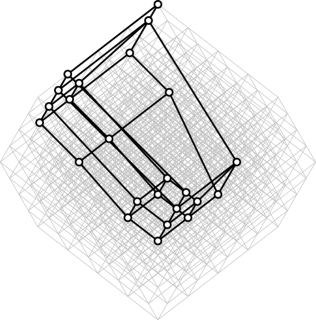
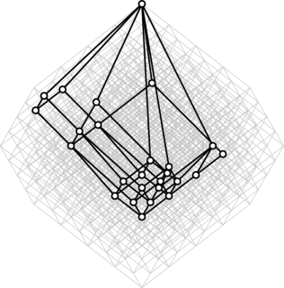
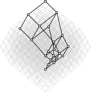
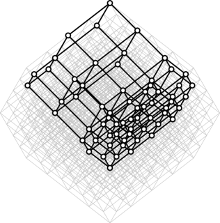
Figure 3: Systems of fixed points of ${}^{{\shortdownarrow_{I}}{\shortuparrow_{I}}}$ from Example 2.

Note that in the terminology of formal concept analysis [28] of data with fuzzy attributes [3, 46, 52], the table in Fig. 2 represents an $\mathbf{L}$-context with the set $X$ of object being the types of leisure activities, the set $Y$ of attributes being properties/features of the activities, and the $\mathbf{L}$-relation $I$ representing the presence of properties by degrees taken from the real unit interval, e.g.,

$$I(\text{beach holiday},\text{happy adults})=0.75$$

means “beach holiday makes adults happy at least to degree $0.75$.” In the examples below, we assume that $\mathbf{L}$ (our structure of degrees) is a complete residuated lattice on $L=\{0,0.25,0.5,0.75,1\}$ with the Gödel operations, i.e., $\wedge$ and $\otimes$ coincide with the minimum, $\vee$ coincides with the maximum, and $a\rightarrow b=b$ for $a>b$ and $a\rightarrow b=1$ for $a\leq b$, cf. (5) and (10).

Given this data, we may be interested in discovering dependencies between the presence of attributes to be able to answer questions like “Does a low cost holiday make parents happy (and to what degree)?” We show by examples that non-redundant bases which describe all such dependencies present in data as well as their systems of models, which can be seen as systems of clusters found in the data [28], are directly influenced by the choice of a parameterization.

Example 2.

(a) Consider $S_{1}=\{\langle\boldsymbol{1},\boldsymbol{1}\rangle,\langle\boldsymbol{f}_{\!0.5\otimes},\boldsymbol{g}_{0.5\rightarrow}\rangle\}$ where $\boldsymbol{f}_{\!0.5\otimes}$ and $\boldsymbol{g}_{0.5\rightarrow}$ are defined by (49) and (50), respectively. This parameterization agrees with a parameterization by a hedge with fixed points $0$, $0.5$, and $1$. In this case, the set of FAIs given by Theorem 15 which is $\mathbf{S}_{1}$-complete in $\langle X,Y,I\rangle$ is also an $\mathbf{S}_{1}$-base and consists of $11$ formulas:

$$\Sigma_{I}=\{ \{k,{}^{0.25\!}/l,{}^{0.75\!}/a,{}^{0.25\!}/e\}\,{\Rightarrow}\,\{k,{}^{0.25\!}/l,a,{}^{0.25\!}/e\},$$

$$\{{}^{0.75\!}/k,{}^{0.25\!}/l,a,{}^{0.25\!}/e\}\,{\Rightarrow}\,\{k,{}^{0.25\!}/l,a,{}^{0.25\!}/e\},$$

$$\{{}^{0.75\!}/k,{}^{0.25\!}/l,{}^{0.5\!}/a,{}^{0.25\!}/e\}\,{\Rightarrow}\,\{{}^{0.75\!}/k,{}^{0.25\!}/l,{}^{0.75\!}/a,{}^{0.25\!}/e\},$$

$$\{{}^{0.5\!}/k,{}^{0.25\!}/l,{}^{0.75\!}/a,{}^{0.25\!}/e\}\,{\Rightarrow}\,\{{}^{0.75\!}/k,{}^{0.25\!}/l,{}^{0.75\!}/a,{}^{0.25\!}/e\},$$

$$\{{}^{0.5\!}/k,{}^{0.25\!}/l,{}^{0.5\!}/a,{}^{0.75\!}/e\}\,{\Rightarrow}\,\{k,{}^{0.25\!}/l,a,e\},$$

$$\{{}^{0.25\!}/k,l,{}^{0.5\!}/a,{}^{0.75\!}/e\}\,{\Rightarrow}\,\{{}^{0.25\!}/k,l,{}^{0.5\!}/a,e\},$$

$$\{{}^{0.25\!}/k,{}^{0.75\!}/l,{}^{0.5\!}/a,e\}\,{\Rightarrow}\,\{{}^{0.25\!}/k,l,{}^{0.5\!}/a,e\},$$

$$\{{}^{0.25\!}/k,{}^{0.5\!}/l,{}^{0.25\!}/a,{}^{0.25\!}/e\}\,{\Rightarrow}\,\{{}^{0.25\!}/k,{}^{0.75\!}/l,{}^{0.5\!}/a,{}^{0.75\!}/e\},$$

$$\{{}^{0.25\!}/k,{}^{0.25\!}/l,{}^{0.75\!}/a,{}^{0.5\!}/e\}\,{\Rightarrow}\,\{{}^{0.25\!}/k,{}^{0.25\!}/l,a,{}^{0.75\!}/e\},$$

$$\{{}^{0.25\!}/k,{}^{0.25\!}/l,{}^{0.25\!}/a,{}^{0.5\!}/e\}\,{\Rightarrow}\,\{{}^{0.25\!}/k,{}^{0.25\!}/l,{}^{0.5\!}/a,{}^{0.5\!}/e\},$$

$$0_{Y}\,{\Rightarrow}\,\{{}^{0.25\!}/k,{}^{0.25\!}/l,{}^{0.25\!}/a,{}^{0.25\!}/e\}\}.$$

The $\mathbf{S}_{1}$-base can be presented in a more compact way by removing superfluous attributes from antecedents and consequents of formulas. That is, for each $A\Rightarrow B$ in $\Sigma_{I}$, we may take minimal $A^{\prime},B^{\prime}\in L^{Y}$ such that $A^{\prime}\subseteq A$ and $B^{\prime}\subseteq B$ and $\Sigma^{\prime}_{I}=\{A^{\prime}\Rightarrow B^{\prime};A\Rightarrow B\in\Sigma_{I}\}$ is $\mathbf{S}_{1}$-complete in $\langle X,Y,I\rangle$. For instance,

$$\Sigma^{\prime}_{I}=\{ \{k,{}^{0.5\!}/a\}\,{\Rightarrow}\,\{a\},\{{}^{0.5\!}/k,a\}\,{\Rightarrow}\,\{k\},\{{}^{0.75\!}/k,{}^{0.5\!}/a\}\,{\Rightarrow}\,\{{}^{0.75\!}/a\},\{{}^{0.5\!}/k,{}^{0.75\!}/a\}\,{\Rightarrow}\,\{{}^{0.75\!}/k\},$$

$$\{{}^{0.5\!}/k,{}^{0.75\!}/e\}\,{\Rightarrow}\,\{{}^{0.75\!}/a,e\},\{l\}\,{\Rightarrow}\,\{e\},\{{}^{0.5\!}/l,e\}\,{\Rightarrow}\,\{l\},\{{}^{0.5\!}/l\}\,{\Rightarrow}\,\{{}^{0.75\!}/l,{}^{0.75\!}/e\},$$

$$\{{}^{0.75\!}/a,{}^{0.5\!}/e\}\,{\Rightarrow}\,\{a,{}^{0.75\!}/e\},\{{}^{0.5\!}/e\}\,{\Rightarrow}\,\{{}^{0.5\!}/a\},0_{Y}\,{\Rightarrow}\,\{{}^{0.25\!}/k,{}^{0.25\!}/l,{}^{0.25\!}/a,{}^{0.25\!}/e\}\}$$

is an $\mathbf{S}_{1}$-base obtained from $\Sigma_{I}$ this way. Let us note that according to Theorem 12, in order to check that $\Sigma^{\prime}_{I}$ is an $\mathbf{S}_{1}$-base, it suffices to check that $[{\cdots}]^{\mathbf{S}_{1}}_{\Sigma^{\prime}_{I}}$ and ${}^{{\shortdownarrow_{I}}{\shortuparrow_{I}}}$ have the same fixed points. This can be done by enumerating the fixed points by algorithms as in [5]. Recall that the fixed points are $\mathbf{L}$-sets of attributes and play the role of conceptual clusters found in the data, see Remark 4. For this particular $\langle X,Y,I\rangle$, $\mathbf{L}$, and $\mathbf{S}_{1}$, there are $22$ distinct fixed points (clusters) of ${}^{{\shortdownarrow_{I}}{\shortuparrow_{I}}}$. Fig. 3 (upper left) depicts the clusters by a Hasse diagram (circled vertices and bold edges) drawn in the space $\langle L^{Y},\subseteq\rangle$ of all $\mathbf{L}$-sets (a hypercube with $|L|^{|Y|}=5^{4}=625$ nodes drawn in gray).

(b) By taking $S_{2}=\{\langle\boldsymbol{1},\boldsymbol{1}\rangle,\langle\boldsymbol{f}_{\!C\otimes},\boldsymbol{g}_{C\rightarrow}\rangle\}$ for $C=\{k,{}^{0.5\!}/a,{}^{0.5\!}/e\}$, we introduce a parameterization which can be seen as a refinement of that in (a). Described verbally, $I\models^{\mathbf{S}_{1}}A\Rightarrow B$ means that, for each activity $x$, if the activity has all the properties in $A$ (fully or at least to degree $0.5$), then it has all the properties in $B$ (fully or at least to degree $0.5$). In contrast, $\mathbf{S}_{2}$ puts more emphasis on “happy kids” (attribute $k$) because $C(k)=1>0.5$ and disregards the cost (attribute $l$) because $C(l)=0<0.5$. Thus, by using such a constraint, a user puts more/less emphasis on certain attributes. An $\mathbf{S}_{2}$-base obtained as in (a) has $15$ FAIs, and ${}^{{\shortdownarrow_{I}}{\shortuparrow_{I}}}$ has $28$ fixed points, see Fig. 3 (upper middle).

(c) Considering $S_{3}$ as in (b) for $C=\{k,{}^{0.75\!}/a,{}^{0.25\!}/e\}$, we put more emphasis on “happy adults” and less emphasis on “easy travel” than in case of (b). In this setting, an $\mathbf{S}_{3}$-base consists of $12$ FAIs and ${}^{{\shortdownarrow_{I}}{\shortuparrow_{I}}}$ has $24$ fixed points, see Fig. 3 (upper right).

(d) Parameterizations with completely different semantics than in (a)–(c) result by considering permutations of attributes. For example, take $S_{4}=\{\langle\boldsymbol{1},\boldsymbol{1}\rangle,\langle\boldsymbol{f}_{\!\circlearrowleft},\boldsymbol{g}_{\circlearrowleft}\rangle\}$ where $(\boldsymbol{f}_{\!\circlearrowleft}(A))(k)=A(a)$, $(\boldsymbol{f}_{\!\circlearrowleft}(A))(l)=A(e)$, $(\boldsymbol{f}_{\!\circlearrowleft}(A))(a)=A(k)$, $(\boldsymbol{f}_{\!\circlearrowleft}(A))(e)=A(l)$ for all $A\in L^{Y}$, and $\boldsymbol{g}_{\circlearrowleft}=\boldsymbol{f}_{\!\circlearrowleft}$ (notice that $\boldsymbol{f}_{\!\circlearrowleft}$ is an involution). Clearly, $\langle\boldsymbol{f}_{\!\circlearrowleft},\boldsymbol{g}_{\circlearrowleft}\rangle$ coincide with (56) and (57) provided that we renumber the attributes $k$, $l$, $a$, and $e$ as $0$, $1$, $2$, and $3$, respectively. Put in words, $I\models^{\mathbf{S}_{1}}A\Rightarrow B$ means that, for each activity $x$, if the activity has all the properties in $A$ (including situations with “happy adults” and “happy kids” interchanged and “low cost” and “easy travel” interchanged), then it has all the properties in $B$ (on the same condition of attibutes being interchanged). In this case, the $\mathbf{S}_{4}$-complete set given by Theorem 15 consists of $17$ implications but unlike the previous cases, the set is redundant. Indeed, $7$ formulas can be removed using Theorem 13 (ii) and Theorem 7 (iv); ${}^{{\shortdownarrow_{I}}{\shortuparrow_{I}}}$ has $26$ fixed points, see Fig. 3 (upper left).

(e) By taking $S_{5}=\{\langle\boldsymbol{1},\boldsymbol{1}\rangle,\langle\boldsymbol{f}_{\!\ominus C},\boldsymbol{g}_{C\oplus}\}$ for $C=\{k,{}^{0.5\!}/a,{}^{0.5\!}/e\}$ with $\boldsymbol{f}_{\!\ominus C}$ and $\boldsymbol{g}_{C\oplus}$ defined by (54) and (55), respectively, we introduce a parameterization $\mathbf{S}_{5}$ which is conceptually similar to $\mathbf{S}_{2}$ but has a different meaning. Indeed, observe that the condition $C\otimes A\subseteq M$ which appears in the definition of $I\models^{\mathbf{S}_{2}}A\Rightarrow B$ reads: For each activity $x$ and each property $y$, $x$ has the property $y$ at least to the degree to which $y$ is in $A$ and $y$ is prescribed by $C$. Analogously for $C\otimes B\subseteq M$. In case of $I\models^{\mathbf{S}_{5}}A\Rightarrow B$, condition $A\ominus C\subseteq M$ reads: For each activity $x$ and each property $y$, $x$ has the property $y$ at most to the degree to which $y$ is in $A$ and $y$ is not prescribed by $C$. It can be shown that if $\mathbf{L}$ is the Łukasiewicz structure of degrees, both types of parameterizations are mutually reducible but not for general $\mathbf{L}$. An $\mathbf{S}_{5}$-base determined by Theorem 15 has $13$ FAIs and ${}^{{\shortdownarrow_{I}}{\shortuparrow_{I}}}$ has $21$ fixed points, see Fig. 3 (lower middle).

(f) Finally, we consider $\mathbf{S}_{6}$ which is generated by $S_{4}\cup S_{5}$, i.e., $\mathbf{S}_{6}$ is a parameterization which combines the constraints on the semantics of FAIs from (d) and (e). Note that in this case, the universe of $S_{6}$ is not the union of $S_{4}$ and $S_{5}$ because the union is not closed under compositions. One may check that $|S_{6}|=8$. An $\mathbf{S}_{6}$-complete set given by Theorem 15 can be reduced to an $\mathbf{S}_{6}$-base consisting of the following formulas (with superfluous attributes removed):

$$\Sigma_{I}=\{ 0_{Y}\,{\Rightarrow}\,\{{}^{0.25\!}/a,{}^{0.25\!}/e\},\{{}^{0.75\!}/l\}\,{\Rightarrow}\,\{{}^{0.75\!}/e\},\{l,{}^{0.75\!}/a\}\,{\Rightarrow}\,\{{}^{0.5\!}/k,e\},\{{}^{0.75\!}/k,{}^{0.5\!}/e\}\,{\Rightarrow}\,\{k\}\}.$$

In this case, ${}^{{\shortdownarrow_{I}}{\shortuparrow_{I}}}$ has $65$ fixed points, cf. Fig. 3 (lower right). We conclude the examples by showing that $\{{}^{0.75\!}/a,e\}\Rightarrow\{{}^{0.5\!}/k,l,a\}$ is semantically entailed by $\Sigma_{I}$ under $\mathbf{S}_{6}$. According to Theorem 18, it suffices to show that $\Sigma_{I}\vdash^{\mathbf{S}_{6}}\{{}^{0.75\!}/a,e\}\Rightarrow\{{}^{0.5\!}/k,l,a\}$ which is indeed the case:

1. $\{l,{}^{0.75\!}/a\}\,{\Rightarrow}\,\{{}^{0.5\!}/k,e\}$ formula in $\Sigma_{I}$,

2. ${\{e,{}^{0.75\!}/k\}\,{\Rightarrow}\,\{l,{}^{0.5\!}/a\}}$ (67) for $\boldsymbol{f}_{\!\circlearrowleft}$ applied to 1,

3. $\{e\}\,{\Rightarrow}\,\{l\}$ (67) for $\boldsymbol{f}_{\!\ominus C}$ with $C=\{k,{}^{0.5\!}/a,{}^{0.5\!}/e\}$ applied to 2,

4. $\{{}^{0.75\!}/a,e\}\,{\Rightarrow}\,\{l,{}^{0.75\!}/a,e\}$ (30) applied to 3 and axiom $\{l,{}^{0.75\!}/a,e\}\,{\Rightarrow}\,\{l,{}^{0.75\!}/a,e\}$,

5. $\{l,{}^{0.75\!}/a\}\,{\Rightarrow}\,\{{}^{0.5\!}/k,e\}$ formula in $\Sigma_{I}$,

6. $\{l,{}^{0.75\!}/a,e\}\,{\Rightarrow}\,\{{}^{0.5\!}/k,l,{}^{0.75\!}/a,e\}$ (30) applied to 5 and $\{{}^{0.5\!}/k,l,{}^{0.75\!}/a,e\}\,{\Rightarrow}\,\{{}^{0.5\!}/k,l,{}^{0.75\!}/a,e\}$,

7. $\{{}^{0.75\!}/a,e\}\,{\Rightarrow}\,\{{}^{0.5\!}/k,l,{}^{0.75\!}/a,e\}$ (30) applied to 4 and 6,

8. $\{{}^{0.75\!}/k,{}^{0.5\!}/e\}\,{\Rightarrow}\,\{k\}$ formula in $\Sigma_{I}$,

9. $\{{}^{0.5\!}/l,{}^{0.75\!}/a\}\,{\Rightarrow}\,\{a\}$ (67) for $\boldsymbol{f}_{\!\circlearrowleft}$ applied to 8,

10. $\{{}^{0.5\!}/k,l,{}^{0.75\!}/a,e\}\,{\Rightarrow}\,\{{}^{0.5\!}/k,l,a,e\}$ (30) applied to 9 and $\{{}^{0.5\!}/k,l,a,e\}\,{\Rightarrow}\,\{{}^{0.5\!}/k,l,a,e\}$,

11. $\{{}^{0.75\!}/a,e\}\,{\Rightarrow}\,\{{}^{0.5\!}/k,l,a,e\}$ (30) applied to 7 and 10,

12. $\{{}^{0.75\!}/a,e\}\,{\Rightarrow}\,\{{}^{0.5\!}/k,l,a\}$ (30) applied to 11 and $\{{}^{0.5\!}/k,l,a,e\}\Rightarrow\{{}^{0.5\!}/k,l,a\}$.

7 Conclusion

General family of if-then rules parameterized by systems of isotone Galois connections has been investigated. Bivalent and graded notions of semantic entailment of if-then rules have been characterized in terms of least models and complete axiomatization has been provided. Non-redundant bases of if-then rules derived from object-attribute data with fuzzy attributes have been characterized using operators on fuzzy sets induced by data. Several examples of parameterizations have been shown. Future research will focus on applications of the parameterizations in formal concept analysis, metods for data dimensionality reduction, and related areas where the earlier parameterizations by hedges have been successfully applied.

Acknowledgment

Supported by grant no. P202/14-11585S of the Czech Science Foundation.

=-4pt

References

- [1] William Ward Armstrong, Dependency structures of data base relationships, Information Processing 74: Proceedings of IFIP Congress (Amsterdam) (J. L. Rosenfeld and H. Freeman, eds.), North Holland, 1974, pp. 580–583.
- [2] Mathias Baaz, Infinite-valued Gödel logics with 0-1 projections and relativizations, GÖDEL ’96, Logical Foundations of Mathematics, Computer Sciences and Physics (Berlin/Heidelberg), Lecture Notes in Logic, vol. 6, Springer-Verlag, 1996, pp. 23–33.
- [3] Radim Belohlavek, Fuzzy Relational Systems: Foundations and Principles, Kluwer Academic Publishers, Norwell, MA, USA, 2002.
- [4] Radim Belohlavek, Bernard De Baets, Jan Outrata, and Vilem Vychodil, Computing the lattice of all fixpoints of a fuzzy closure operator, Fuzzy Systems, IEEE Transactions on 18 (2010), no. 3, 546–557.
- [5] , Computing the lattice of all fixpoints of a fuzzy closure operator, IEEE Transactions on Fuzzy Systems 18 (2010), no. 3, 546–557.
- [6] Radim Belohlavek, Tatana Funiokova, and Vilem Vychodil, Fuzzy closure operators with truth stressers, Logic Journal of IGPL 13 (2005), no. 5, 503–513.
- [7] Radim Belohlavek, Vladimir Sklenar, and Jiri Zacpal, Crisply generated fuzzy concepts, Formal Concept Analysis (Bernhard Ganter and Robert Godin, eds.), Lecture Notes in Computer Science, vol. 3403, Springer Berlin Heidelberg, 2005, pp. 269–284.
- [8] Radim Belohlavek and Vilem Vychodil, Reducing the size of fuzzy concept lattices by hedges, Fuzzy Systems, 2005. FUZZ ’05. The 14th IEEE International Conference on, 2005, pp. 663–668.
- [9] , Attribute implications in a fuzzy setting, Formal Concept Analysis (Rokia Missaoui and Jürg Schmidt, eds.), Lecture Notes in Computer Science, vol. 3874, Springer Berlin Heidelberg, 2006, pp. 45–60.
- [10] , Fuzzy attribute logic over complete residuated lattices, Journal of Experimental & Theoretical Artificial Intelligence 18 (2006), no. 4, 471–480.
- [11] , On proofs and rule of multiplication in fuzzy attribute logic, Foundations of Fuzzy Logic and Soft Computing (P. Melin, O. Castillo, T. Aguilar, L. J. Kacprzyk, and W. Pedrycz, eds.), Lecture Notes in Computer Science, vol. 4529, Springer Berlin Heidelberg, 2007, pp. 471–480.
- [12] , Codd’s relational model from the point of view of fuzzy logic, J. Log. Comput. 21 (2011), no. 5, 851–862.
- [13] , Formal concept analysis and linguistic hedges, International Journal of General Systems 41 (2012), no. 5, 503–532.
- [14] , Attribute dependencies for data with grades, CoRR abs/1402.2071 (2014).
- [15] Garrett Birkhoff, Lattice theory, 1st ed., American Mathematical Society, Providence, 1940.
- [16] Petr Cintula, Petr Hájek, and Carles Noguera (eds.), Handbook of Mathematical Fuzzy Logic, Volume 1, Studies in Logic, Mathematical Logic and Foundations, vol. 37, College Publications, 2011.
- [17] Petr Cintula, Petr Hájek, and Carles Noguera (eds.), Handbook of Mathematical Fuzzy Logic, Volume 2, Studies in Logic, Mathematical Logic and Foundations, vol. 38, College Publications, 2011.
- [18] Carlos Damásio and Luís Pereira, Monotonic and residuated logic programs, Symbolic and Quantitative Approaches to Reasoning with Uncertainty (Salem Benferhat and Philippe Besnard, eds.), Lecture Notes in Computer Science, vol. 2143, Springer Berlin / Heidelberg, 2001, pp. 748–759.
- [19] Brian A. Davey and Hilary A. Priestley, Introduction to Lattices and Order, Cambridge University Press, Cambridge, 1990.
- [20] Bernard De Baets and Radko Mesiar, Triangular norms on product lattices, Fuzzy Sets Syst. 104 (1999), no. 1, 61–75.
- [21] Robert P. Dilworth, Abstract residuation over lattices, Bull. Amer. Math. Soc. 44 (1938), 262–268.
- [22] Didier Dubois, Eyke Hüllermeier, and Henri Prade, A systematic approach to the assessment of fuzzy association rules, Data Min. Knowl. Discov. 13 (2006), no. 2, 167–192.
- [23] Francesc Esteva and Lluís Godo, Monoidal t-norm based logic: Towards a logic for left-continuous t-norms, Fuzzy Sets and Systems 124 (2001), no. 3, 271–288.
- [24] Francesc Esteva, Lluís Godo, Petr Hájek, and Mirko Navara, Residuated fuzzy logics with an involutive negation, Archive for Mathematical Logic 39 (2000), no. 2, 103–124.
- [25] Francesc Esteva, Lluís Godo, and Carles Noguera, A logical approach to fuzzy truth hedges, Information Sciences 232 (2013), 366–385.
- [26] Nikolaos Galatos, Peter Jipsen, Tomacz Kowalski, and Hiroakira Ono, Residuated Lattices: An Algebraic Glimpse at Substructural Logics, Volume 151, 1st ed., Elsevier Science, San Diego, USA, 2007.
- [27] Bernhard Ganter, Two basic algorithms in concept analysis, Proceedings of the 8th International Conference on Formal Concept Analysis (Berlin, Heidelberg), ICFCA’10, Springer-Verlag, 2010, pp. 312–340.
- [28] Bernhard Ganter and Rudolf Wille, Formal concept analysis: Mathematical foundations, 1st ed., Springer-Verlag New York, Inc., Secaucus, NJ, USA, 1997.
- [29] George Georgescu and Andrei Popescu, Non-dual fuzzy connections, Archive for Mathematical Logic 43 (2004), no. 8, 1009–1039.
- [30] Giangiacomo Gerla, Fuzzy Logic. Mathematical Tools for Approximate Reasoning, Kluwer Academic Publishers, Dordrecht, The Netherlands, 2001.
- [31] Joseph A. Goguen, -fuzzy sets, Journal of Mathematical Analysis and Applications 18 (1967), no. 1, 145–174.
- [32] , The logic of inexact concepts, Synthese 19 (1979), 325–373.
- [33] Siegfried Gottwald, Mathematical fuzzy logics, Bulletin of Symbolic Logic 14 (2008), no. 2, 210–239.
- [34] Jean-Louis Guigues and Vincent Duquenne, Familles minimales d’implications informatives resultant d’un tableau de données binaires, Math. Sci. Humaines 95 (1986), 5–18.
- [35] Petr Hájek, Metamathematics of Fuzzy Logic, Kluwer Academic Publishers, Dordrecht, The Netherlands, 1998.
- [36] , On very true, Fuzzy Sets and Systems 124 (2001), no. 3, 329–333.
- [37] Petr Hájek and Jeff Paris, A dialogue on fuzzy logic, Soft Computing 1 (1997), no. 1, 3–5.
- [38] Ulrich Höhle, Monoidal logic, Fuzzy-Systems in Computer Science (R. Kruse, J. Gebhardt, and R. Palm, eds.), Artificial Intelligence / Künstliche Intelligenz, Vieweg+Teubner Verlag, 1994, pp. 233–243.
- [39] Richard Holzer, Knowledge acquisition under incomplete knowledge using methods from formal concept analysis: Part I, Fundamenta Informaticae 63 (2004), no. 1, 17–39.
- [40] Erich Peter Klement, Radko Mesiar, and Endre Pap, Triangular Norms, 1 ed., Springer, 2000.
- [41] George J. Klir and Bo Yuan, Fuzzy Sets and Fuzzy Logic: Theory and Applications, Prentice-Hall, Inc., Upper Saddle River, NJ, USA, 1995.
- [42] Stanislav Krajči, Cluster based efficient generation of fuzzy concepts, Neural Network World (2003), no. 5, 521–530.
- [43] Tomas Kuhr and Vilem Vychodil, Fuzzy logic programming reduced to reasoning with attribute implications, Fuzzy Sets and Systems (2014), in press, DOI 10.1016/j.fss.2014.04.013.
- [44] John W. Lloyd, Foundations of Logic Programming, Springer-Verlag New York, Inc., New York, NY, USA, 1984.
- [45] David Maier, Theory of Relational Databases, Computer Science Pr, Rockville, MD, USA, 1983.
- [46] Jesús Medina, Manuel Ojeda-Aciego, and Jorge Ruiz-Calviño, Formal concept analysis via multi-adjoint concept lattices, Fuzzy Sets and Systems 160 (2009), no. 2, 130–144.
- [47] Vilém Novák, Irina Perfilieva, and Jiří Močkoř, Mathematical Principles of Fuzzy Fogic, Kluwer Academic Publishers, Boston, MA, USA, 1999.
- [48] Ewa Orłowska and Anna Radzikowska, Double residuated lattices and their applications, Revised Papers from the 6th International Conference and 1st Workshop of COST Action 274 TARSKI on Relational Methods in Computer Science (London, UK, UK), ReIMICS ’01, Springer-Verlag, 2002, pp. 171–189.
- [49] Jan Pavelka, On fuzzy logic I: Many-valued rules of inference, Mathematical Logic Quarterly 25 (1979), no. 3–6, 45–52.
- [50] , On fuzzy logic II: Enriched residuated lattices and semantics of propositional calculi, Mathematical Logic Quarterly 25 (1979), no. 7–12, 119–134.
- [51] , On fuzzy logic III: Semantical completeness of some many-valued propositional calculi, Mathematical Logic Quarterly 25 (1979), no. 25–29, 447–464.
- [52] Silke Pollandt, Fuzzy-Begriffe: Formale Begriffsanalyse unscharfer Daten, Springer, 1997.
- [53] Gaisi Takeuti and Satoko Titani, Globalization of intuitionistic set theory, Annals of Pure and Applied Logic 33 (1987), 195–211.
- [54] Alfred Tarski, A lattice-theoretical fixpoint theorem and its applications, Pacific Journal of Mathematics 5 (1955), 285–309.
- [55] Maarten H. Van Emden and Robert A. Kowalski, The semantics of predicate logic as a programming language, J. ACM 23 (1976), no. 4, 733–742.
- [56] Vilem Vychodil, Fuzzy attribute implications and their expressive power, International Journal of Uncertainty, Fuzziness and Knowledge-Based Systems 21 (2013), no. 4, 483–496.
- [57] Morgan Ward and Robert P. Dilworth, Residuated lattices, Trans. Amer. Math. Soc. 45 (1939), 335–354.
- [58] Wolfgang Wechler, Universal Algebra for Computer Scientists, EATCS Monographs on Theoretical Computer Science, vol. 25, Springer-Verlag, Berlin Heidelberg, 1992.
- [59] Sadok Ben Yahia and Ali Jaoua, Data Mining and Computational Intelligence (Janusz Kacprzyk, Abraham Kandel, Mark Last, and Horst Bunke, eds.), Physica-Verlag GmbH, Heidelberg, Germany, Germany, 2001, pp. 167–190.
- [60] Lotfi A. Zadeh, Fuzzy sets, Information and Control 8 (1965), no. 3, 338–353.
- [61] , A fuzzy-set-theoretic interpretation of linguistic hedges, Journal of Cybernetics 2 (1972), no. 3, 4–34.
- [62] , The concept of a linguistic variable and its application to approximate reasoning–I, Information Sciences 8 (1975), no. 3, 199–249.
- [63] , The concept of a linguistic variable and its application to approximate reasoning–II, Information Sciences 8 (1975), no. 4, 301–357.
- [64] , The concept of a linguistic variable and its application to approximate reasoning–III, Information Sciences 9 (1975), no. 1, 43–80.
- [65] , Toward a theory of fuzzy information granulation and its centrality in human reasoning and fuzzy logic, Fuzzy Sets and Systems 90 (1997), no. 2, 111–127.
- [66] , Is there a need for fuzzy logic?, Information Sciences 178 (2008), no. 13, 2751–2779.