Success and Failure of Adaptation-Diffusion Algorithms
for Consensus in Multi-Agent Networks

Abstract

This paper investigates the problem of distributed stochastic approximation in multi-agent systems. The algorithm under study consists of two steps: a local stochastic approximation step and a diffusion step which drives the network to a consensus. The diffusion step uses row-stochastic matrices to weight the network exchanges. As opposed to previous works, exchange matrices are not supposed to be doubly stochastic, and may also depend on the past estimate.

We prove that non-doubly stochastic matrices generally influence the limit points of the algorithm. Nevertheless, the limit points are not affected by the choice of the matrices provided that the latter are doubly-stochastic in expectation. This conclusion legitimates the use of broadcast-like diffusion protocols, which are easier to implement. Next, by means of a central limit theorem, we prove that doubly stochastic protocols perform asymptotically as well as centralized algorithms and we quantify the degradation caused by the use of non doubly stochastic matrices. Throughout the paper, a special emphasis is put on the special case of distributed non-convex optimization as an illustration of our results.

I INTRODUCTION

Distributed stochastic approximation has been recently proposed using different cooperative approaches. In the so-called incremental approach (see for instance [1, 2, 3, 4]) a message containing an estimate of the quantity of interest iteratively travels all over the network. This paper focuses on another cooperative approach based on average consensus techniques where the estimates computed locally by each agent are combined through the network.

Consider a network composed by $N$ agents, or nodes. Agents seek to find a consensus on some global parameter by means of local observations and peer-to-peer communications. The aim of this paper is to analyze the behavior of the following distributed algorithm. Node $i$ ($i=1,\dots,N$) generates a ${\mathbb{R}}^{d}$-valued stochastic process $(\theta_{n,i})_{n\geq 0}$. At time $n$, the update is in two steps:
[Local step] Node $i$ generates a temporary iterate $\tilde{\theta}_{n,i}$ given by

$$\tilde{\theta}_{n,i}=\theta_{n-1,i}+\gamma_{n}\,Y_{n,i}\ ,$$ (1)

where $\gamma_{n}$ is a deterministic positive step size and where the ${\mathbb{R}}^{d}$-valued random process $(Y_{n,i})_{n\geq 1}$ represents the observations made by agent $i$.
[Gossip step] Node $i$ is able to observe the values $\tilde{\theta}_{n,j}$ of some other $j$’s and computes the weighted average:

$$\theta_{n,i}=\sum_{j=1}^{N}w_{n}(i,j)\,\tilde{\theta}_{n,j}\ ,$$ (2)

where the $w_{n}(i,j)$’s are scalar non-negative random coefficients such that $\sum_{j=1}^{N}w_{n}(i,j)=1$ for any $i$. The sequence of random matrices $W_{n}:=[w_{n}(i,j)]_{i,j=1}^{N}$ represents the time-varying communication network between the nodes. One simply set $w_{n}(i,j)=0$ whenever nodes $i$ and $j$ are unable to communicate at time $n$. The aim of this paper is to investigate the almost sure (a.s.) convergence of this algorithm as $n$ tends to infinity as well as the convergence rate. Our goal is in particular to quantify the effect of the sequence of matrices $(W_{n})_{n\geq 1}$ on the convergence. The algorithm is initialized at some arbitrary ${\mathbb{R}}^{d}$-valued vectors $\theta_{0,1},\cdots,\theta_{0,N}$.

Application to distributed optimization. The algorithm (1)-(2) under study is not new. The idea beyond the algorithm traces back to [5, 6] where a network of processors seeks to optimize some objective function known by all agents (possibly up to some additive noise). More recently, numerous works extended this kind of algorithm to more involved multi-agent scenarios, see [7, 8, 9, 10, 11, 12, 13, 14, 15, 16, 17, 18, 19] as a non-exhaustive list. In this context, one seeks to minimize a sum of local private cost functions $f_{i}$ of the agents:

$$\min_{\theta\in{\mathbb{R}}^{d}}\ \sum_{i=1}^{N}f_{i}(\theta)\ ,$$ (3)

where for all $i$, the function $f_{i}$ is supposed to be unknown by any other agent $j,j\neq i$. To address this question, it is assumed that

$$Y_{n,i}=-\nabla f_{i}(\theta_{n-1,i})+\xi_{n,i}$$ (4)

where $\nabla$ is the gradient operator and $\xi_{n,i}$ represents some random perturbation which possibly occurs when observing the gradient. In this paper, we handle the case where functions $f_{i}$ are not necessarily convex. Of course, in that case, there is generally no hope to ensure the convergence to a minimizer to (3). Instead, a more realistic objective is to achieve critical points of the objective function i.e., points $\theta$ such that $\sum_{i}\nabla f_{i}(\theta)=0$.

Convergence to a global minimizer is shown in [20] assuming convex utility functions and bounded (sub)gradients. The results of [20] are extended in [21] to the stochastic descent case i.e., when the observation of utility functions is perturbed by a random noise. More recently, [14] investigated distributed stochastic approximation at large, providing stability conditions of the algorithm (1)-(2) while relaxing the bounded gradient assumption and including the case of random communication links. In [14], it is also proved under some hypotheses that the estimation error is asymptotically normal: the convergence rate and the asymptotic covariance matrix are characterized. An enhanced averaging algorithm à la Polyak is also proposed to recover the optimal convergence rate.

Doubly and non-doubly stochastic matrices. In most works (see for instance [20, 21, 22]), the matrices $(W_{n})_{n\geq 1}$ are assumed doubly stochastic, meaning that $W_{n}^{T}{\boldsymbol{1}}=W_{n}{\boldsymbol{1}}={\boldsymbol{1}}$ where ${\boldsymbol{1}}$ is the $N\times 1$ vector whose components are all equal to one and where ^T denotes transposition. Although row-stochasticity ($W_{n}{\boldsymbol{1}}={\boldsymbol{1}}$) is rather easy to ensure in practice, column-stochasticity ($W_{n}^{T}{\boldsymbol{1}}={\boldsymbol{1}}$) implies more stringent restrictions on the communication protocol. For instance, in [23], each one-way transmission from an agent $i$ to another agent $j$ requires at the same time a feedback link from $j$ to $i$. As a matter of fact, double stochasticity prevents from using natural broadcast schemes, in which a given node may transmit its local estimate to all neighbors without expecting any immediate feedback.

Remarkably, although generally assumed, double stochasticity of the matrices $W_{n}$ is in fact not mandatory. A couple of works (see e.g. [24, 14]) get rid of the column-stochasticity condition, but at the price of assumptions that may not always be satisfied in practice. Other works ([25, 17, 26]) manage to circumvent the use of feedback links by coupling the gradient descent with the so-called push-sum protocol [27]. The latter however introduces an additional communication of weights in the network in order to keep track of some summary of the past transmissions. In this paper, we address the following questions: What conditions on the sequence $(W_{n})_{n\geq 1}$ are needed to ensure that Algorithm (1)-(2) drives all agents to a common critical point of $\sum_{i}f_{i}$? What happens if these conditions are not satisfied? How is the convergence rate influenced by the communication protocol?

Contributions.

1. Assuming that $(W_{n})_{n\geq 1}$ forms an independent and identically distributed (i.i.d.) sequence of stochastic matrices, we prove under some technical hypotheses that Algorithm (1)-(2) leads the agents to a consensus, which is characterized. It is shown that the latter consensus does not necessarily coincide with a critical point of $\sum_{i}f_{i}$.

2. We provide sufficient conditions either on the communication protocol $(W_{n})_{n\geq 1}$ or on the functions $f_{i}$ which ensure that limit points are the critical points of $\sum_{i}f_{i}$.

3. When such conditions are not satisfied, we also propose a simple modification of the algorithm which allows to recover the sought behavior.

4. We extend our results to a broader setting, assuming that the matrices $(W_{n})_{n\geq 1}$ are no longer i.i.d., but are likely to depend on both the current observations and the past estimates. We also investigate a general stochastic approximation framework which goes beyond the model (4) and beyond the only problem of distributed optimization.

5. We characterize the convergence rate of the algorithm under the form of a central limit theorem. Unlike [14], we address the case where the sequence $(W_{n})_{n\geq 1}$ is not necessarily doubly stochastic. We show that non-doubly stochastic matrix have an influence on the asymptotic error covariance (even if they are doubly stochastic in average). On the other hand, we prove that when the matrix $W_{n}$ is doubly stochastic for all $n$, the asymptotic covariance is identical to the one obtained in a centralized setting.

The paper is organized as follows. Section II is a gentle presentation of our results in the special case of distributed optimization (see (3)) assuming in addition that sequence $(W_{n})$ is i.i.d. In Section III we provide the general setting to study almost sure convergence. Almost sure convergence is studied in Section IV. Section V investigates convergence rates. Conclusions and numerical results complete the paper.

Notations: Throughout the paper, the vectors are column vectors. The random variables $W_{n}\in{\mathbb{R}}^{N\times N}$ and $Y_{n}:=(Y_{n,1}^{T},\dots,Y_{n,N}^{T})^{T}\in{\mathbb{R}}^{dN}$, $n\geq 1$, are defined on the same measurable space equipped with a probability ${\mathbb{P}}$; ${\mathbb{E}}$ denotes the associated expectation. For any $n\geq 1$, define the $\sigma$-field ${\mathcal{F}}_{n}:=\sigma({\theta}_{0},W_{1},\dots,W_{n},Y_{1},\dots,Y_{n})$ where $\theta_{0}$ is the (possibly random) initial point of the algorithm.
It is assumed that for any $i\in 1,\dots,N$, $(\theta_{n,i})_{n\geq 0}$ satisfies the update equations (1)-(2); and we set

$$\theta_{n}:=(\theta_{n,1}^{T},\dots,\theta_{n,N}^{T})^{T}.$$

For any vector $x\in{\mathbb{R}}^{\ell}$, $|x|$ represents the Euclidean norm of $x$. $I_{N}$ is the $N\times N$ identity matrix. $J:={\boldsymbol{1}}{\boldsymbol{1}}^{T}/N$ denotes the orthogonal projector onto the linear span of the all-one $N\times 1$ vector ${\boldsymbol{1}}$, and ${J_{\bot}}:=I_{N}-J$. We denote by $\otimes$ the Kronecker product between matrices. For a matrix $A$, the spectral norm is denoted by $\|A\|$ and the spectral radius is denoted by $r(A)$ whenever $A$ is a square matrix.

II Distributed Optimization

II-A Framework

We first sketch our result in the special case of distributed optimization i.e., when the “innovation” $Y_{n,i}$ of the algorithm in (1) has the form (4).

Assumption 1.

1. $f_{i}:{\mathbb{R}}^{d}\to{\mathbb{R}}$ is differentiable and $\nabla f_{i}$ is locally Lipschitz-continuous.

2. For any Borel set A of ${\mathbb{R}}^{dN}$, ${\mathbb{P}}\left[\xi_{n+1}\in A\,|\,{\mathcal{F}}_{n}\right]=\nu_{\theta_{n}}(A)$ almost surely (a.s.) where $(\nu_{\theta})_{\theta\in{\mathbb{R}}^{dN}}$ is a family of probability measures such that $\int z\,d\nu_{\theta}(z)=0$ and $\sup\limits_{\theta\in{\mathcal{K}}}\int|z|^{2}d\nu_{\theta}(z)<\infty$ for any compact set ${\mathcal{K}}\subset{\mathbb{R}}^{dN}$ .

For simplicity, the matrix-valued process $W_{n}$ will be assumed i.i.d. and independent of both processes $Y_{n}$ and $\theta_{n}$. This assumption will be relaxed in section III.

Assumption 2.

1. For any $n\geq 0$, conditionally to ${\mathcal{F}}_{n}$, $(Y_{n+1},W_{n+1})$ are independent.

2. $(W_{n})_{n\geq 1}$ is an i.i.d. sequence of row-stochastic matrices (i.e., $W_{n}{\boldsymbol{1}}={\boldsymbol{1}}$ for any $n$) with non-negative entries.

3. The spectral radius of the matrix ${\mathbb{E}}[W_{1}^{T}J_{\bot}W_{1}]$ is strictly lower than $1$.

The row-stochasticity assumption is a rather mild condition. In many works, it is also assumed that $W_{n}$ is column-stochastic i.e., $\sum_{i}w_{n}(i,j)=1$ for any $j$, though this assumption is not required in this work. Assumption 2-3) is a contraction condition which is required to drive the network to a consensus.

Assumption 3.

The deterministic step-size sequence $(\gamma_{n})_{n\geq 1}$ satisfies $\gamma_{n}>0$ and:

1. $\lim_{n}\gamma_{n+1}/\gamma_{n}\ =1$,

2. $\sum_{n}\gamma_{n}=+\infty$, $\sum_{n}\gamma_{n}^{1+\lambda}<\infty$ for some $\lambda\in(0,1)$,

3. $\sum_{n}|\gamma_{n}-\gamma_{n-1}|<\infty$ .

Polynomially decreasing sequences $\gamma_{n}\sim\gamma_{\star}/n^{a}$ when $n\to\infty$, for some $a\in(1/2,1]$ and $\gamma_{\star}>0$ satisfy Assumption 3. Finally, we introduce a stability-like condition.

Assumption 4.

Almost surely, there exists a compact set ${\mathcal{K}}$ of ${\mathbb{R}}^{dN}$ such that $\theta_{n}\in{\mathcal{K}}$ for any $n\geq 0$.

Assumption 4 claims that the sequence $(\theta_{n})_{n\geq 0}$ remains in a compact set and this compact set may depend on the path. It is implied by the stronger assumption “there exists a compact set ${\mathcal{K}}$ of ${\mathbb{R}}^{dN}$ such that with probability one, $\theta_{n}\in{\mathcal{K}}$ for any $n\geq 0$”. Checking Assumption 4 is not always an easy task. As the main scope of this paper is the analysis of convergence rather than stability, it is taken for granted: we refer to [14] for sufficient conditions implying stability.

II-B Results

The following lemma follows from standard algebra.

Lemma 1.

Under Assumptions 2-2) and 2-3), the $N\times 1$ vector $v$ defined by $v^{T}:=\frac{1}{N}{\boldsymbol{1}}^{T}\overline{W}(I_{N}-J_{\bot}\overline{W})^{-1}$ is the unique non-negative vector satisfying $v^{T}=v^{T}\overline{W}$ and $v^{T}{\boldsymbol{1}}=1$.

If $A$ is a set, we say that $(x_{n})_{n}$ converges to $A$ if $\inf\{|x_{n}-y|:y\in A\}$ tends to zero as $n\to\infty$.

Theorem 1.

Let Assumptions 1, 2, 3 and  4 hold true. Define the function $V:{\mathbb{R}}^{d}\to{\mathbb{R}}$

$$V(\theta):=\sum_{i=1}^{N}v_{i}\,f_{i}(\theta)\,$$ (5)

where $v=(v_{1},\dots,v_{N})$ is the vector defined in Lemma 1. Assume that the set ${\mathcal{L}}=\{\theta\in{\mathbb{R}}^{d}\,|\,\nabla V=0\}$ of critical points of $V$ is non-empty and included in some level set $\{\theta:V(\theta)\leq C\}$, and that $V({\mathcal{L}})$ has an empty interior. Assume also that the level sets $\{\theta:V(\theta)\leq C\}$ are either empty or compact. The following holds with probability one:

1. The algorithm converges to a consensus i.e., $\lim_{n\to\infty}\max_{i,j}|\theta_{n,i}-\theta_{n,j}|=0$.

2. The sequence $(\theta_{n,1})_{n\geq 0}$ converges to ${\mathcal{L}}$ as $n\to\infty$.

Theorem 1 is proved in Appendix A. Its proof consists in showing that it is a special case of the more general convergence result given by Theorem 2.

II-C Success and Failure of Convergence

The algorithm converges to ${\mathcal{L}}$ which in general is not the set of the critical points of $\theta\mapsto\sum_{i}f_{i}(\theta)$. We discuss some special where both sets actually coincide.

Scenario 1. All functions $f_{i}$ are strictly convex and admit a (unique) common minimizer $\theta_{\star}$.

This case is for instance investigated by [13] in the framework of statistical estimation in wireless sensor network. The set ${\mathcal{L}}$ is formed by the minimizers of $\,\sum_{i}f_{i}$. Relaxing strict convexity, note that when the functions $f_{i}$ are just convex with a common minimizer and $v_{i}>0$ for any $i$, then ${\mathcal{L}}$ is formed by the minimizers of $\sum_{i}f_{i}$, then the same conclusion holds.

Scenario 2. $\overline{W}$ is column-stochastic i.e., ${\boldsymbol{1}}^{T}\overline{W}={\boldsymbol{1}}^{T}$ .

In this case, $v$ given by Lemma 1 is the vector $\frac{1}{N}{\boldsymbol{1}}$. Consequently, $V=\frac{1}{N}\sum_{i}f_{i}$. Here again, ${\mathcal{L}}$ is the set of minimizers of $\sum_{i}f_{i}$. An example of random communication protocol (see [28]) satisfying ${\boldsymbol{1}}^{T}\overline{W}={\boldsymbol{1}}^{T}$ is the following: at time $n$, a single node $i$ wakes up at random with probability $p_{i}$ and broadcasts its temporary update $\tilde{\theta}_{n,i}$ to all its neighbors ${\mathcal{N}}_{i}$. Any neighbor $j$ computes the weighted average $\theta_{n,j}=\beta\tilde{\theta}_{n,i}+(1-\beta)\tilde{\theta}_{n,j}$. On the other hand, any node $k$ which does not belong to the neighborhood of $i$ (including $i$ itself) sets $\theta_{n,k}=\tilde{\theta}_{n,k}$. Then, given $i$ wakes up, the $(k,\ell)$th entry of $W_{n}$ is given by:

$$w_{n}(k,\ell)=\left\{\begin{array}[h]{ll}1&\textrm{if }k\notin{\mathcal{N}}_{i}\textrm{ and }k=\ell\ ,\\ \beta&\textrm{if }k\in{\mathcal{N}}_{i}\textrm{ and }\ell=i\ ,\\ 1-\beta&\textrm{if }k\in{\mathcal{N}}_{i}\textrm{ and }k=\ell\ ,\\ 0&\textrm{otherwise.}\end{array}\right.$$

Here, $W_{n}$ is not doubly stochastic. However, when nodes wake up according to the uniform distribution ($p_{i}=\frac{1}{N}$ for all $i$) it is easily seen that ${\boldsymbol{1}}^{T}{\mathbb{E}}[W_{n}]={\boldsymbol{1}}^{T}$.

II-D Enhanced Algorithm with Weighted Step Sizes

We end up this section with a simple modification of the initial algorithm in the case where $v_{i}>0$ for all $i$. Let us replace the local step (1) of the algorithm by

$$\tilde{\theta}_{n,i}:=\theta_{n-1,i}+\gamma_{n}\,v_{i}^{-1}Y_{n,i}$$ (6)

where $Y_{n,i}$ is still given by (4). As an immediate Corollary of Theorem 1, the algorithm (6)-(2) drives the agent to a consensus which coincides with the critical points of $\sum_{i}f_{i}$.

Of course, this modification requires for each node $i$ to have some prior knowledge of the communication protocol through the coefficients $v_{i}$ (in that case, questions related to a distributed computation of the $v_{i}$’s would be of interest, but are beyond the scope of this paper).

III Distributed Robbins-Monro Algorithm: General Setting

In this section, we consider the general setting described by Algorithm (1)-(2) with weaker conditions on the distribution of the observations $Y_{n}$. We also weaken the assumptions on $(Y_{n+1},W_{n+1})$: our general framework includes the case when the communication protocol is adapted at each time $n$.

We denote by $\mathsf{M}_{1}$ the set of $N\times N$ non-negative row-stochastic matrices and we endow $\mathsf{M}_{1}$ with its Borel $\sigma$-field.

Assumption 5.

1. There exists a collection of distributions $\left(\mu_{\theta}\right)_{\theta\in{\mathbb{R}}^{dN}}$ on ${\mathbb{R}}^{dN}\times\mathsf{M}_{1}$ such that a.s. for any Borel set $A$:

   $${\mathbb{P}}\left[(Y_{n+1},W_{n+1})\in A\,|\,{\mathcal{F}}_{n}\right]=\mu_{\theta_{n}}(A)\ .$$

   In addition, the application $\theta\mapsto\mu_{\theta}(A)$ defined on ${\mathbb{R}}^{dN}$ is measurable for any $A$ in the Borel $\sigma$-field of ${\mathbb{R}}^{dN}\times\mathsf{M}_{1}$.

2. For any compact set ${\mathcal{K}}\subset{\mathbb{R}}^{dN}$, $\sup\limits_{\theta\in{\mathcal{K}}}\int|y|^{2}d\mu_{\theta}(y,w)<\infty$.

Assumption 5-1) means that the joint distribution of the r.v.’s $Y_{n+1}$ and $W_{n+1}$ depends on the past ${\mathcal{F}}_{n}$ only through the last value $\theta_{n}$ of the vector of estimates. It also implies that $W_{n}$ is almost-surely (a.s.) non-negative and row-stochastic. Since the variables $(Y_{n+1},W_{n+1})$ are not necessarily independent conditionally to the past $\mathcal{F}_{n}$ and $(W_{n})_{n\geq 1}$ are no longer i.i.d., the contraction condition on $J_{\bot}W_{1}$ is replaced with the following condition:

Assumption 6.

For any compact set ${\mathcal{K}}\subset{\mathbb{R}}^{dN}$, there exists $\rho_{\mathcal{K}}\in(0,1)$ such that for all $\theta\in{\mathcal{K}}$, $\phi$ in $\mathbb{R}^{dN}$ and $A\in{\mathbb{R}}^{dN}\times{\mathbb{R}}^{dN}$,

$$\int|((J_{\bot}w)\otimes I_{d})(\phi+Ay)|^{2}d\mu_{\theta}(y,w)\leq\rho_{{\mathcal{K}}}\!\!\int\!\!|\phi+Ay|^{2}\,d\mu_{\theta}(y,w)\,.$$

Assumption 6 is satisfied as soon as the spectral radius $r\left({\mathbb{E}}\left[W_{1}^{T}{J_{\bot}}W_{1}|\theta_{0},Y_{1}\right]\right)$ is upper bounded by a constant independent of $(\theta_{0},Y_{1})$ when $\theta_{0}\in{\mathcal{K}}$ and strictly lower than one. When $(W_{n})_{n\geq 1}$ is an i.i.d. sequence, independent of the sequence $(Y_{n})_{n\geq 1}$ and of $\theta_{0}$, the above condition reduces to $r({\mathbb{E}}[W_{1}^{T}{J_{\bot}}W_{1}])<1$.

IV Convergence Analysis

For any vector ${x}\in{\mathbb{R}}^{dN}$ of the form $x=(x_{1}^{T},\dots,x_{N}^{T})^{T}$ where $x_{i}\in{\mathbb{R}}^{d}$, we define the vector of ${\mathbb{R}}^{d}$ $\langle x\rangle:=(x_{1}+\cdots+x_{N})/N=({{\boldsymbol{1}}^{T}\otimes I_{d}})x/N$. We extend the notation to matrices $X\in{\mathbb{R}}^{dN\times k}$ as $\langle X\rangle=\frac{1}{N}({{\boldsymbol{1}}^{T}\otimes I_{d}})X$. We note ${\mathcal{J}}:=J\otimes I_{d}$ and ${\mathcal{J}}_{\bot}:=J_{\bot}\otimes I_{d}$. Note that ${\mathcal{J}}x=\boldsymbol{1}\otimes\langle x\rangle$ . Algorithm (1-2) can be written in matrix form as:

$$\theta_{n}=\mathcal{W}_{n}\left(\theta_{n-1}+\gamma_{n}Y_{n}\right)\quad\text{where}\quad\mathcal{W}_{n}=W_{n}\otimes I_{d}\,.$$ (7)

We decompose the estimate vector $\theta_{n}$ into two components $\theta_{n}=\boldsymbol{1}\otimes\langle\theta_{n}\rangle+{\mathcal{J}}_{\bot}\theta_{n}$. In Section IV-A, we analyze the asymptotic behavior of the disagreement vector ${\mathcal{J}}_{\bot}\theta_{n}$. The study of the average vector $\langle\theta_{n}\rangle$ will be addressed in Section IV-B. These two sections are prefaced by a result which established the dynamics of these sequences. Set $\alpha_{n}:=\gamma_{n}/\gamma_{n+1}$ and

$$\phi_{n}:=\gamma_{n+1}^{-1}\,{\mathcal{J}}_{\bot}\theta_{n}\,.$$ (8)

The following lemma is left to the reader.

Lemma 2.

For each $n$, let $\theta_{n}$ be given by (7) and let $W_{n}$ be row stochastic. Then,

$$\langle{\theta}_{n}\rangle =\langle{\theta}_{n-1}\rangle+\gamma_{n}\langle{\cal W}_{n}(Y_{n}+\phi_{n-1})\rangle\ ,$$ (9)

$$\phi_{n} =\alpha_{n}\,{\mathcal{J}}_{\bot}{\cal W}_{n}(\phi_{n-1}+Y_{n})\,.$$ (10)

IV-A Disagreement Vector

Lemma 3.

Let Assumptions 3-1),  5 and 6 hold. Let $(\phi_{n})_{n\geq 0}$ be the sequence given by (8). For any compact set ${\mathcal{K}}\subset{\mathbb{R}}^{dN}$, $\sup_{n}{\mathbb{E}}\left(|\phi_{n}|^{2}\mathbb{I}_{\bigcap_{j\leq n-1}\{\theta_{j}\in{\mathcal{K}}\}}\right)<\infty$.

The result is proved in Appendix B. This lemma implies that for any compact set, there exists $C$ such that for any $n\geq 0$, ${\mathbb{E}}[|{\mathcal{J}}_{\bot}\theta_{n}|^{2}\mathbb{I}_{\bigcap_{k}\{\theta_{k}\in{\mathcal{K}}_{m}\}}]\leq C\gamma_{n+1}^{2}$.

Proposition 1 (Agreement).

Under Assumptions 3-1),  3-2),  4,  5 and 6, $\lim_{n\to\infty}{\mathcal{J}}_{\bot}\theta_{n}=0$ a.s.

Proof.

Let $({\mathcal{K}}_{m})_{m\geq 0}$ be an increasing sequence of compact subsets of ${\mathbb{R}}^{dN}$ such that $\bigcup_{m}{\mathcal{K}}_{m}={\mathbb{R}}^{dN}$. Under Assumption 4, we have to prove equivalently that for any $m\geq 0$, $\lim_{n}{\mathcal{J}}_{\bot}\theta_{n}{\boldsymbol{1}}_{\bigcap_{k}\{\theta_{k}\in{\mathcal{K}}_{m}\}}=0$ a.s. Let $m\geq 0$. Lemma 3 implies that there exists a constant $C$ such that for any $n$, ${\mathbb{E}}[|{\mathcal{J}}_{\bot}\theta_{n}|^{2}\mathbb{I}_{\bigcap_{k}\{\theta_{k}\in{\mathcal{K}}_{m}\}}]\leq C\gamma_{n+1}^{2}$. By Assumption 3-2), this implies that $\sum_{n}{\mathbb{E}}[|{\mathcal{J}}_{\bot}\theta_{n}|^{2}\mathbb{I}_{\bigcap_{k}\{\theta_{k}\in{\mathcal{K}}_{m}\}}]$ is finite; hence $\sum_{n}|{\mathcal{J}}_{\bot}\theta_{n}|^{2}\mathbb{I}_{\bigcap_{k}\{\theta_{k}\in{\mathcal{K}}_{m}\}}$ is finite a.s. which yields $\lim_{n}{\mathcal{J}}_{\bot}\theta_{n}^{2}\mathbb{I}_{\bigcap_{k}\{\theta_{k}\in{\mathcal{K}}_{m}\}}=0$ a.s. ∎

IV-B Average vector

We now study the long-time behavior of the average estimate $\langle\theta_{n}\rangle$. Define for any $\theta\in{\mathbb{R}}^{dN}$:

$$\overline{\mathcal{W}}_{\theta} := \int\left(w\otimes I_{d}\right)\,d\mu_{{\theta}}(y,w)$$ (11)

$$z_{\theta} := \int(w\otimes I_{d})y\,d\mu_{{\theta}}(y,w)\,.$$ (12)

and let us assume regularity-in-$\theta$ properties of these quantities

Assumption 7.

There exists $\lambda_{\mu}\in(1/2,1]$ and for any compact set ${\mathcal{K}}\subset{\mathbb{R}}^{dN}$, there exists a constant $C>0$ such that for any $\theta,\theta^{\prime}\in{\mathcal{K}}$,

$$\left\|\overline{\mathcal{W}}_{\theta}-\overline{\mathcal{W}}_{{\theta}^{\prime}}\right\|\leq C|{\theta}-{\theta}^{\prime}|^{\lambda_{\mu}}\,,$$ (13)

$$\left|{\mathcal{J}}z_{\theta}-{\mathcal{J}}z_{{\mathcal{J}}{\theta}}\right|\leq C|{{\mathcal{J}}_{\bot}}{\theta}|^{\lambda_{\mu}}\,,$$ (14)

$$\left|{\mathcal{J}}_{\bot}z_{\theta}-{\mathcal{J}}_{\bot}z_{{\theta}^{\prime}}\right|\leq C|{\theta}-{\theta}^{\prime}|^{\lambda_{\mu}}\,,$$ (15)

We define the mean field function $h:{\mathbb{R}}^{d}\to{\mathbb{R}}^{d}$ (10) by

$$h(\vartheta)=\langle z_{{\boldsymbol{1}}\otimes\vartheta}+\overline{\mathcal{W}}_{{\boldsymbol{1}}\otimes\vartheta}\,m_{{\boldsymbol{1}}\otimes\vartheta}^{(1)}\rangle$$ (16)

where $m_{{\boldsymbol{1}}\otimes\vartheta}^{(1)}$ is the expectation of the invariant distribution $\pi_{1,{\boldsymbol{1}}\otimes\vartheta}$, given by (see Proposition 4 in Appendix C)

$$m^{(1)}_{\theta}:=(I_{dN}-{{\mathcal{J}}_{\bot}}\overline{\mathcal{W}}_{\theta})^{-1}{{\mathcal{J}}_{\bot}}z_{\theta}\,.$$

Note that under Assumption 6, this quantity is well defined since for any compact ${\mathcal{K}}\subset{\mathbb{R}}^{dN}$, $\sup_{\theta\in{\mathcal{K}}}\|{\mathcal{J}}_{\bot}\overline{\mathcal{W}}_{\theta}\|\leq\sqrt{\rho_{\mathcal{K}}}$.

Assumption 8.

1. $h:{\mathbb{R}}^{d}\to{\mathbb{R}}^{d}$ is continuous.

2. There exists a continuously differentiable function $V:{\mathbb{R}}^{d}\to{\mathbb{R}}^{+}$ such that

   1. there exists $M>0$ such that ${\mathcal{L}}=\{\vartheta\in{\mathbb{R}}^{d}:\nabla V^{T}(\vartheta)h(\vartheta)=0\}\subset\{V\leq M\}$. In addition, $V({\mathcal{L}})$ has an empty interior;

   2. there exists $M^{\prime}>M$ such that $\{V\leq M^{\prime}\}$ is a compact subset of ${\mathbb{R}}^{d}$;

   3. for any $\vartheta\in{\mathbb{R}}^{d}\setminus{\mathcal{L}}$, $\nabla V^{T}(\vartheta)h(\vartheta)<0$.

Assumptions 5, 6 and 7 imply that $\vartheta\mapsto m^{(1)}_{{\boldsymbol{1}}\otimes\vartheta}$ is continuous on ${\mathbb{R}}^{d}$ (see Proposition 5 in Appendix C). Therefore, a sufficient condition for the Assumption 8-1) is to strengthen the conditions (14-15) of Assumption 7 as follows: $\left|z_{\theta}-z_{{\theta}^{\prime}}\right|\leq C|{\theta}-{\theta}^{\prime}|^{\lambda_{\mu}}$.

Proposition 2.

Let Assumptions 3, 4, 5, 6,7 and 8 hold true. Assume in addition that $\lambda\leq\lambda_{\mu}$ where $\lambda,\lambda_{\mu}$ are resp. given by Assumption 3 and 7. The average sequence $(\langle\theta_{n}\rangle)_{n}$ converges almost-surely to a connected component of ${\mathcal{L}}$.

The proof of Proposition 2 is given in Appendix D. It consists in verifying the assumptions of [29, Theorem 2].

IV-C Main Convergence Result

As a trivial consequence of Propositions 1 and 2, we have

Theorem 2.

Let Assumptions 3, 4, 5, 6, 7 and 8 hold true. Assume in addition that $\lambda\leq\lambda_{\mu}$ where $\lambda,\lambda_{\mu}$ are resp. given by Assumption 3 and 7. The following holds with probability one:

1. The algorithm converges to a consensus i.e., $\lim_{n\to\infty}{{\mathcal{J}}_{\bot}}{\theta}_{n}=0$;

2. $\theta_{n,1}$ converges to a connected component of ${\mathcal{L}}$.

V Convergence Rate

V-A Main Result

We derive the rate of convergence of the sequence $\{\theta_{n},n\geq 0\}$ to ${\boldsymbol{1}}\otimes\theta_{\star}$ for some $\theta_{\star}$ satisfying

Assumption 9.

$\theta_{\star}$ is a root of $h$ i.e., $h(\theta_{\star})=0$. Moreover, $h$ is twice continuously differentiable in a neighborhood of $\theta_{\star}$. The Jacobian $\nabla h(\theta_{\star})$ is a Hurwitz matrix. Denote by $-L$, $L>0$, the largest real part of its eigenvalues.

The moment conditions on the conditional distributions of the observations $Y_{n}$ and the contraction assumption on the network have to be strengthened as follows:

Assumption 10.

There exists $\tau\in(0,2)$ such that for any compact set ${\mathcal{K}}\subset{\mathbb{R}}^{dN}$, one has $\sup_{\theta\in{\mathcal{K}}}\int|y|^{2+\tau}\ d\mu_{\theta}(y,w)<\infty$.

Assumption 11.

Let $\tau$ be given by Assumption 10. For any compact set ${\mathcal{K}}\subset{\mathbb{R}}^{dN}$, there exists $\tilde{\rho}_{\mathcal{K}}\in(0,1)$ such that for any $\phi\in{\mathbb{R}}^{dN}$

$$\sup_{\theta\in{\mathcal{K}}}\int|((J_{\bot}w)\otimes I_{d})|^{2+\tau}d\mu_{\theta}(y,w)\leq\tilde{\rho}_{\mathcal{K}}\ |\phi|^{2+\tau}\ .$$

We also go further in the regularity-in-$\theta$ of the integrals w.r.t. $\mu_{\theta}$. More precisely

Assumption 12.

There exists $\lambda_{\mu}\in(1/2,1]$ and for any compact set ${\mathcal{K}}\subset{\mathbb{R}}^{dN}$ there exists a constant $C$ such that

1. for any $\theta,\theta^{\prime}\in{\mathcal{K}}$, $\left|\langle z_{\theta}\rangle-\langle z_{\theta^{\prime}}\rangle\right|\leq C\left|\theta-\theta^{\prime}\right|^{\lambda_{\mu}}$.

2. Set $\mathcal{Q}_{A}(x,y,w):=(x+y)^{\text{{t}}}(w\otimes I_{d})^{\text{{t}}}{\mathcal{J}}_{\bot}A{\mathcal{J}}_{\bot}(w\otimes I_{d})(x+y)$ for some $dN\times dN$ matrix $A$. For any $\theta,\theta^{\prime}\in{\mathcal{K}}$, $x\in{\mathbb{R}}^{dN}$ and any matrix $A$ such that $\|A\|\leq 1$,

   $$\left|\int\mathcal{Q}_{A}(x,y,w)d\mu_{\theta}(y,w)-\mathcal{Q}_{A}(x,y,w)d\mu_{\theta^{\prime}}(y,w)\ \right|\\ \leq C\,\left|\theta-\theta^{\prime}\right|^{\lambda_{\mu}}\ (1+|x|^{2})\ .$$

We finally have to strengthen the conditions on the step-size sequence.

Assumption 13.

Let $\tau$ (resp. $\lambda_{\mu}$) be given by Assumption 10 (resp. Assumption 12). As $n\to\infty$, $\gamma_{n}\sim\gamma_{\star}/n^{a}$ for some $a\in((1+\lambda_{\mu})^{-1}\vee(1+\tau/2)^{-1};1]$ and $\gamma_{\star}>0$. In addition, if $a=1$ then $\gamma_{\star}>1/(2L)$ where $L$ is given by Assumption 9.

Define $m^{(1)}_{\star}:=(I_{dN}-{{\mathcal{J}}_{\bot}}\overline{\mathcal{W}}_{{\boldsymbol{1}}\otimes\theta_{\star}})^{-1}{{\mathcal{J}}_{\bot}}z_{{\boldsymbol{1}}\otimes\theta_{\star}}$ and $m^{(2)}_{\star}:=\left(I_{d^{2}N^{2}}-\Phi_{\star}\right)^{-1}\zeta_{\star}$ where $z_{\theta}$ is defined in (12), where

$$\Phi_{\star} := \int T(w)\,d\mu_{{\boldsymbol{1}}\otimes\theta_{\star}}(y,w)$$

$$\zeta_{\star} := \int T(w)\text{vec}\,\left(yy^{T}+2m^{(1)}_{\star}y^{T}\right)\,d\mu_{{\boldsymbol{1}}\otimes\theta_{\star}}(y,w)$$

and where we used the notation $T(w):=(({J_{\bot}}w)\otimes I_{d})\otimes(({J_{\bot}}w)\otimes I_{d})$. As will be seen in the proofs, $m^{(1)}_{\star}$ and $m^{(2)}_{\star}$ represent the asymptotic first order moment and (vectorized) second order moment of the r.v. $\phi_{n}$ defined by (8). Define also $R_{\star}(w):=(w\otimes I_{d})-\overline{\mathcal{W}}_{{\boldsymbol{1}}\otimes\theta_{\star}}$ and $\upsilon_{\star}(y,w):=(w\otimes I_{d})y-z_{{\boldsymbol{1}}\otimes\theta_{\star}}$. Finally, define

$${\mathsf{A}}_{\star} :=\left(\frac{{\boldsymbol{1}}^{T}}{N}\otimes I_{d}\right)(I_{dN}+\overline{\mathcal{W}}_{{\boldsymbol{1}}\otimes\theta_{\star}}(I_{dN}-{{\mathcal{J}}_{\bot}}\overline{\mathcal{W}}_{{\boldsymbol{1}}\otimes\theta_{\star}})^{-1}{{\mathcal{J}}_{\bot}})$$

$${\mathcal{R}}_{\star} :=\int(R_{\star}(w)\otimes R_{\star}(w))\ d\mu_{{\boldsymbol{1}}\otimes\theta_{\star}}(y,w)$$

$${\mathcal{T}}_{\star} :=\int(\upsilon_{\star}(y,w)\otimes R_{\star}(w))d\mu_{{\boldsymbol{1}}\otimes\theta_{\star}}(y,w)$$

$${\mathcal{S}}_{\star} :=\int\text{vec}\,(\upsilon_{\star}(y,w)\upsilon_{\star}(y,w)^{T})d\mu_{{\boldsymbol{1}}\otimes\theta_{\star}}(y,w)\,.$$

We establish in Section E the following result.

Theorem 3.

Let Assumption 5-1), Assumption 7, Assumption 6 and Assumption 9 to Assumption 13 hold true. Let $U_{\star}$ be the positive-definite matrix given by

$$\text{vec}\,U_{\star}=({\mathsf{A}}_{\star}\otimes{\mathsf{A}}_{\star})({\mathcal{R}}_{\star}\,m^{(2)}_{\star}+2{\mathcal{T}}_{\star}m^{(1)}_{\star}+{\mathcal{S}}_{\star})$$

Then conditionally to the event $\{\lim_{n}\theta_{n}={\boldsymbol{1}}\otimes\theta_{\star}\}$, the sequence $\{\gamma_{n}^{-1/2}(\langle\theta_{n}\rangle-\theta_{\star}),n\geq 0\}$ converges in distribution to a zero mean Gaussian distribution with covariance matrix $\mathsf{V}$ where $\mathsf{V}$ is the unique positive-definite matrix satisfying

$$\mathsf{V}\nabla h(\theta_{\star})^{T}+\nabla h(\theta_{\star})\mathsf{V}=-U_{\star}\quad\text{if $a<1$,}$$

$$\mathsf{V}\left(I_{d}+2\gamma_{\star}\nabla h(\theta_{\star})\right)^{T}+\left(I_{d}+2\gamma_{\star}\nabla h(\theta_{\star})\right)\mathsf{V}=-2\gamma_{\star}U_{\star}\quad\text{if $a=1$.}$$

V-B A Special Case: Doubly-Stochastic Matrices

In this paragraph, let us investigate the special case when $(W_{n})_{n}$ are $N\times N$ doubly-stochastic matrices. Note that in this case, (9) gets into $\langle\theta_{n}\rangle=\langle\theta_{n-1}\rangle+\gamma_{n}\langle Y_{n}\rangle$ and the mean field function $h$ is equal to $h(\vartheta)=\int\langle y\rangle d\mu_{{\boldsymbol{1}}\otimes\vartheta}(y,w)$. Since $W_{n}$ is column-stochastic, $\int w\,d\mu_{{\boldsymbol{1}}\otimes\theta_{\star}}(y,w)$ is column-stochastic, and we have ${\mathsf{A}}_{\star}=\frac{{\boldsymbol{1}}^{T}}{N}\otimes I_{d}$. Then, it is not difficult to check that ${\mathsf{A}}_{\star}R_{\star}(w)=0$, which implies that ${\mathcal{R}}_{\star}={\mathcal{T}}_{\star}=0$. This yields the following corollary

Corollary 1.

In addition to the assumptions of Theorem 3, assume that $(W_{n})_{n}$ are $N\times N$ doubly-stochastic matrices and set $\bar{y}_{\star}=\int y\,d\mu_{{\boldsymbol{1}}\otimes\theta_{\star}}(y,w)$. Then

$$U_{\star}=\int\langle y-\bar{y}_{\star}\rangle\langle y-\bar{y}_{\star}\rangle^{T}d\mu_{{\boldsymbol{1}}\otimes\theta_{\star}}(y,w)\,.$$

VI Concluding remarks

In this paragraph, we informally draw some general conclusions of our study. We assimilate the communication protocol to the selection of the sequence $W_{n}$, which we assume i.i.d. in this paragraph for simplicity. We say that a protocol is doubly stochastic if $W_{n}$ is doubly stochastic for each $n$. We say that a protocol is doubly stochastic in average if ${\mathbb{E}}\left[W_{n}\right]$ is doubly stochastic for each $n$.

1. Consensus is fast. Theorem 3 states that the average estimation error converges to zero at rate $\sqrt{\gamma_{n}}$. This result was actually expected, as $\sqrt{\gamma_{n}}$ is the well-known convergence rate of standard stochastic approximation algorithms.

   On the other hand, Lemma 3 suggests that the disagreement vector ${{\mathcal{J}}_{\bot}}\theta_{n}$ goes to zero at rate $\gamma_{n}$ that is, one order of magnitude faster. Asymptotically, the fluctuations of the normalized estimation error $(\theta_{n}-{\boldsymbol{1}}\otimes\theta_{\star})/\sqrt{\gamma_{n}}$ are fully supported by the consensus space.

   This remark also suggests to analyze non-stationary communication protocols, for which the number of transmissions per unit of time decreases with $n$. This problem is addressed in [14].

2. Non-doubly stochastic protocols generally influence the limit points. This issue is discussed in Section II-C. The choice of the matrices $W_{n}$ is likely to have an impact on the set of limit points of the algorithms. This may be inconvenient especially in distributed optimization tasks.

3. Protocols that are doubly stochastic ”in average” all lead to the same limit points. In the framework of distributed optimization, the latter set of limit points precisely coincides with the sought critical points of the minimization problem. It means that non-doubly stochastic protocols can be used provided that they are doubly stochastic in average.

4. Asymptotically, doubly stochastic protocols perform as well as a centralized algorithm. By Corollary 1, if $W_{n}$ is chosen to be doubly stochastic for all $n$, the asympotic error covariance characterized in Theorem 3 does not depend on the specific choice of $W_{n}$. In distributed optimization, the asymptotic performance is identical to the performance that would have been obtained by replacing $W_{n}$ by the orthogonal projector $J$, which would lead to the centralized update $\langle\theta_{n}\rangle=\langle\theta_{n-1}\rangle+\frac{\gamma_{n}}{N}\sum_{i=1}^{N}Y_{n,i}\,.$ On the opposite, protocols that are not doubly stochastic generally influence the asymptotic error covariance, even if they are doubly stochastic in average.

VII Numerical Results

We illustrate the convergence results obtained in Section II-B and discussed in sections II-C and VI. We depict a particular case of the distributed optimization problem described in Section II. Consider a network of $N=5$ agents and for any $i=1,\dots,5$, we define a private cost function $f_{i}:{\mathbb{R}}\to{\mathbb{R}}$. We address the following minimization problem:

$$\min_{\theta\subset{\mathbb{R}}}\,\sum_{i=1}^{5}\frac{1}{2}(\theta-\alpha_{i})^{2}$$ (17)

where $\alpha^{T}=(-3,5,5,1,-3)$. The minimizer of (17) is $\theta_{f}=\langle\alpha\rangle=1$. The network is represented by an undirected graph $G=(V,E)$ with vertices $\{1,\dots,N\}$ and $6$ fixed edges $E$. The corresponding adjacency matrix is given by

$$A=\begin{pmatrix}0&1&0&1&0\\ 1&0&1&0&0\\ 0&1&0&1&1\\ 1&0&1&0&1\\ 0&0&1&1&0\end{pmatrix}.$$

We choose $\theta_{0,i}=0$ for each agent $i$ and the step-size sequence of the form $\gamma_{n}=0.1/n^{0.7}$. Observations $Y_{n,i}$ are defined as in (4): $(\xi_{n,i})_{n,i}$ is an i.i.d. sequence with Gaussian distribution ${\cal N}(0,\sigma^{2})$ where $\sigma^{2}=1$.

Figure 1 illustrates the two results of Theorem 1 according to different gossip matrices $(W_{n})_{n}$. First, Figure 1 (a) addresses the convergence of sequence $(\theta_{n,1})_{n\geq 0}$ as a function of $n$ to show the influence of matrices $W_{n}$ to the limit points. In particular, the dashed line curve corresponds to the algorithm (1)-(2) when $W_{n}$ is assumed to be fixed and deterministic ($W_{n}=W_{1}$ for all $n$); we select $W_{1}$ in such a way that each agent computes the average of the temporary estimates in its neighborhood. This is equivalent to set $W_{1}=(I_{N}+D)^{-1}(I_{N}+A)$, where $D$ is the diagonal matrix containing the degrees, i.e. $D(i,i)=\sum_{j=1}^{N}A(i,j)$ for each agent $i$. Note that $W_{1}$ is not doubly stochastic since ${\boldsymbol{1}}^{T}W_{1}\neq{\boldsymbol{1}}^{T}$. Computing the left Perron eigenvector defined by Lemma 1 yields the minimizer of $V=\sum_{i}v_{i}f_{i}$ being $\theta_{V}=v^{T}\alpha=1.24$. In that case, the sequence $(\theta_{n,1})_{n}$ converges to $\theta_{\star}=\theta_{V}$ instead of the desired $\theta_{\star}=\theta_{f}$. Figure 1 (a) includes the trajectory of $\theta_{n,1}$ generated by Algorithm (6)-(2) with $W_{1}=(I_{N}+D)^{-1}(I_{N}+A)$. As proposed in Section II-D when introducing the weighted step size such $\gamma_{n}v_{i}^{-1}$ the sequence now converge to the sought value $\theta_{f}$.

(a) Trajectories of $\theta_{n,1}$ as a function of $n$.

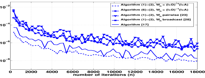
(b) $\sqrt{\frac{1}{N}\sum_{i=1}^{N}(\theta_{n,i}-\langle{\theta}_{n}\rangle)^{2}}$ as a function of $n$.

Figure 1: Convergence result of Theorem 1 according to different communication schemes for $(W_{n})_{n}$.

Figure 1 (a) also illustrates the convergence behavior of Scenario 2 where the limit point $\theta_{\star}$ of Algorithm (1)-(2) corresponds with $\theta_{f}$. In that case, we consider two standard models for $W_{n}$, namely the pairwise gossip of [23] and the broadcast gossip of [28] (we set $\beta=\frac{1}{2}$). Finally, the plain line in Figure 1 (a) shows the performance of the algorithm proposed by [17] for distributed optimization which is based on a synchronous version of the push-sum model of [27].

We conclude the illustration of Theorem 1 by the results on the consensus convergence for the same examples of $W_{n}$ considered in Figure 1 (a). Thus, Figure 1 (b) represents the norm of the scaled disagreement vector as a function of $n$. As expected from Theorem 1-2), consensus is asymptotically achieved independently of the limit point, i.e. $\theta_{f}$ or $\theta_{V}$. Note that the synchronous models of $W_{1}$ and [17] require $N$ transmissions at each iteration $n$ whereas the gossip protocols of [23] and [28] only require two and one transmissions respectively due to their asynchronous nature. This may explain the gap between the curves in Figure 1 (b) when regarding the convergence rate towards the consensus.

The result of Theorem 3 is illustrated in Figure 2 which leads to the concluding remark 4) of Section VI. Figures 2 (a) and 2 (b) display the asymptotic analysis of the normalized average error $\gamma_{n}^{-1/2}(\langle\theta_{n}\rangle-\theta^{\star})$. Indeed, once the convergence is achieved, the asymptotic distribution can be characterized by the closed form of the variance $U^{\star}\in{\mathbb{R}}$. In this example, Theorem 3 states that $\gamma_{n}^{-1/2}(\langle\theta_{n}\rangle-\theta^{\star})$ converges in distribution to a r.v. $\sim\mathcal{N}(0,\mathsf{V})$ where $\nabla h(\theta_{\star})=-1$ and thus the variance is $\mathsf{V}=\frac{U_{\star}}{2}$. The first boxplot and the first histogram in Figure 2 are related to the algorithm implemented in a centralized manner. We consider the distributed algorithm (1)-(2) with different choices of $W_{n}$: the pairwise gossip of [23], the broadcast gossip of [28] and the fixed $W_{1}$ defined by $(I_{N}+D)^{-1}(I_{N}+A)$. The normal distribution obtained in Theorem 3 is coherent with the empirical results.

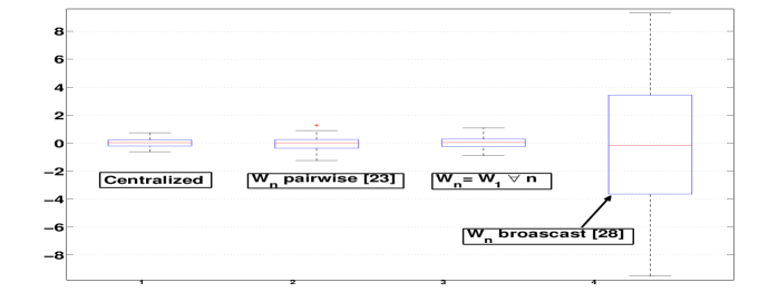
(a) Boxplots of the normalized average error.

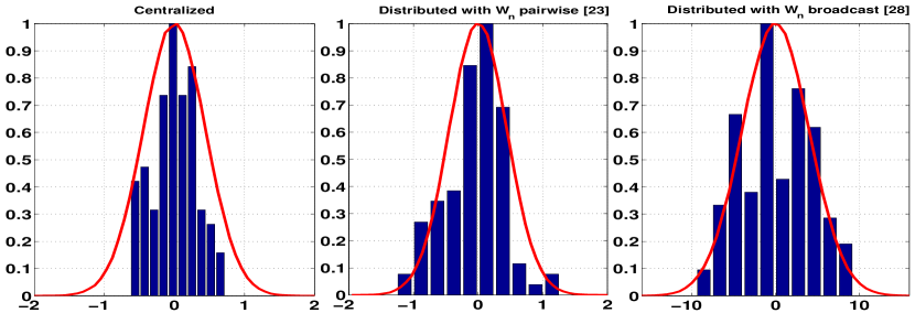
(b) Empirical distribution (dark bars) versus theoretical distribution given by Theorem 3 (solid line).

Figure 2: Asymptotic analysis of the normalized average error $\frac{1}{\sqrt{\gamma_{n}}}(\langle\theta_{n}\rangle-\theta^{\star})$ of Algorithm (1)-(2) according to different communication schemes for $(W_{n})_{n}$ after $n=30000$ iterations and over $100$ independent Monte-Carlo runs.

Appendix A Proof of Theorem 1

We prove that the Assumptions 5 to 8 hold. Then Theorem 1 will follow from Theorem 2. For any $\theta=(\theta_{1},\dots,\theta_{N})\in{\mathbb{R}}^{dN}$ where $\theta_{i}\in{\mathbb{R}}^{d}$, define the ${\mathbb{R}}^{dN}$-valued function $g$ by $g(\theta):=(-\nabla f_{1}(\theta_{1})^{T},\dots,-\nabla f_{N}(\theta_{N})^{T})^{T}$. Under Assumption 2-1) and Assumption 2-2), for any Borel set $A\times B$ of ${\mathbb{R}}^{dN}\times\mathsf{M}_{1}$ ${\mathbb{P}}[(Y_{n+1},W_{n+1})\in A\times B|{\mathcal{F}}_{n}]={\mathbb{P}}[Y_{n+1}\in A|{\mathcal{F}}_{n}]{\mathbb{P}}[W_{n+1}\in B]$. In addition, by Assumption 1 and Eq. (4) ${\mathbb{P}}[Y_{n+1}\in A|{\mathcal{F}}_{n}]=\int\mathbb{I}_{A}\left(g(\theta_{n})+z\right)\ d\nu_{\theta_{n}}(z)\,.$ The above discussion provides the expression of $\mu_{\theta}$ in Assumption 5-1). In addition, under Assumption 1-2), for any compact set ${\mathcal{K}}$ of ${\mathbb{R}}^{dN}$,

$$\sup_{\theta\in{\mathcal{K}}}\int|y|^{2}d\mu_{\theta}(y,w)=\sup_{\theta\in{\mathcal{K}}}\left(|g(\theta)|^{2}+\int|z|^{2}d\nu_{\theta}(z)\right)<\infty$$

which proves Assumption 5-2). Assumption 6 easily follows from Assumption 2-3). The regularity conditions of Assumption 7 are satisfied with $\lambda_{\mu}=\delta$, where $\delta$ is given by Assumption 1. Observe indeed that the left hand side of (13) is zero and (14) and (15) are true as long as $(\nabla f_{i})_{i}$ are locally Hölder-continuous. Again, the expression of $\mu_{\theta}$ implies that $\overline{\mathcal{W}}_{\theta}={\mathbb{E}}\left[{\cal W}_{1}\right]$. Therefore, $h(\vartheta)=\langle{\mathbb{E}}[{\cal W}_{1}]\,g\left({\boldsymbol{1}}\otimes\vartheta\right)\rangle=-\sum_{i=1}^{N}v_{i}\nabla f_{i}(\vartheta)$ which completes the proof.

Appendix B Proof of Lemma 3

From (10), we compute $|\phi_{n}|^{2}=\alpha_{n}^{2}(\phi_{n-1}+Y_{n})^{T}{\cal W}_{n}^{T}{\mathcal{J}}_{\bot}{\cal W}_{n}(\phi_{n-1}+Y_{n})$. Using Assumption 5-1), ${\mathbb{E}}\left[|\phi_{n}|^{2}|{\mathcal{F}}_{n-1}\right]$ is equal to

$$\alpha_{n}^{2}\ \int(\phi_{n-1}+y)^{T}(w\otimes I_{d}){\mathcal{J}}_{\bot}(w\otimes I_{d})(\phi_{n-1}+y)\ d\mu_{\theta_{n-1}}(y,w)\,.$$

By Fubini Theorem and Assumption 6, there exists $\rho_{\mathcal{K}}\in(0,1)$ such that for any $n\geq 1$, ${\mathbb{E}}\left[|\phi_{n}|^{2}|{\mathcal{F}}_{n-1}\right]\leq\alpha_{n}^{2}\rho_{\mathcal{K}}\int|\phi_{n-1}+y|^{2}d\mu_{\theta_{n-1}}(y,w)$. By Assumption 5-2), there exists a constant $C$ such that for any $n\geq 1$ almost-surely

$${\mathbb{E}}\left[|\phi_{n}|^{2}|{\mathcal{F}}_{n-1}\right]\mathbb{I}_{\theta_{n-1}\in{\mathcal{K}}}\leq\alpha_{n}^{2}\rho_{\mathcal{K}}\left(|\phi_{n-1}|^{2}+2|\phi_{n-1}|\sqrt{C}+C\right)\,.$$

Set $U_{n}:=|\phi_{n}|^{2}\mathbb{I}_{\bigcap_{j\leq n-1}\{\theta_{j}\in{\mathcal{K}}\}}$. Upon noting that $\mathbb{I}_{\bigcap_{j\leq n-1}\{\theta_{j}\in{\mathcal{K}}\}}\leq\mathbb{I}_{\bigcap_{j\leq n-2}\{\theta_{j}\in{\mathcal{K}}\}}$, the previous inequality implies ${\mathbb{E}}[U_{n}]\leq\alpha_{n}^{2}\rho_{\mathcal{K}}\left({\mathbb{E}}\left[U_{n-1}\right]+2\sqrt{{\mathbb{E}}[U_{n-1}]}\,\sqrt{C}+C\right)$. Let $\delta\in(\rho_{\mathcal{K}},1)$. For any $n$ large enough (say $n\geq n_{0}$), $\alpha_{n}^{2}\rho_{\mathcal{K}}\leq 1-\delta$ since $\lim_{n}\alpha_{n}=1$ under Assumption 3-1). There exist positive constants $M,b$ such that for any $n\geq n_{0}$,

$${\mathbb{E}}[U_{n}] \leq\left(1-\delta\right)\left({\mathbb{E}}\left[U_{n-1}\right]+2\sqrt{{\mathbb{E}}[U_{n-1}]}\,\sqrt{C}+C\right)$$

$$\leq\left(1-\frac{\delta}{2}\right){\mathbb{E}}[U_{n-1}]+b{\boldsymbol{1}}_{{\mathbb{E}}[U_{n-1}]\leq M}\,.$$

A trivial induction implies that ${\mathbb{E}}[U_{n}]\leq(1-\delta/2)^{n-n_{0}}{\mathbb{E}}[U_{n_{0}}]+2b/\delta$, which concludes the proof.

Appendix C Preliminary results on the sequence $(\phi_{n})_{n}$

Due to the coupling of the sequences $(\langle{\theta}_{n}\rangle)_{n}$ and $(\phi_{n})_{n}$ (see Eq. (9)), the asymptotic analysis of $(\langle{\theta}_{n}\rangle)_{n}$ requires a more detailed understanding of the behavior of $\phi_{n}$. Note from Assumption 5-1) and (10) that $\{\phi_{n},n\geq 0\}$ is a Markov chain w.r.t. the filtration $\{\mathcal{F}_{n},n\geq 0\}$ with a transition kernel controlled by $\{\alpha_{n},\theta_{n},n\geq 0\}$ (see also (19) below).

Let us introduce some notations and definitions. If $(x,A)\mapsto P(x,A)$ is a probability transition kernel on ${\mathbb{R}}^{dN}$, then for any bounded continuous function $f:{\mathbb{R}}^{dN}\to{\mathbb{R}}$, $Pf$ is the measurable function $x\mapsto\int f(y)P(x,dy)$ . If $\nu$ is a probability on ${\mathbb{R}}^{dN}$, $\nu P$ is the probability on ${\mathbb{R}}^{dN}$ given by $\nu P(A)=\int\nu(dx)\,P(x,A)$. For $n\geq 0$, notation $P^{n}$ stands for the $n$-order iterated kernel i.e., $P^{n}f(x)=\int P^{n-1}f(y)P(x,dy)$; by convention $P^{0}(x,A)={\boldsymbol{1}}_{A}(x)=\delta_{x}(A)$. A measure $\pi$ is said to be an invariant distribution w.r.t. $P$ if $\pi P=\pi$. For $p\geq 0$, denote by ${\mathcal{L}}_{p}({\mathbb{R}}^{dN})$ the set of lipschitz functions $f:{\mathbb{R}}^{dN}\to{\mathbb{R}}^{dN}$ satisfying

$$[f]_{p}:=\sup_{x,y\in{\mathbb{R}}^{dN}}\frac{|f(x)-f(y)|}{|x-y|(1+|x|^{p}+|y|^{p})}<\infty\,.$$

We define $N_{p}(f):=(\sup_{x\in{\mathbb{R}}^{dN}}\frac{|f(x)|}{1+|x|^{p+1}})\vee[f]_{p}$ for $f\in{\mathcal{L}}_{p}({\mathbb{R}}^{dN})$. For any ${\theta}\in{\mathbb{R}}^{dN}$ and any $\alpha\geq 0$, define the probability transition kernel $P_{\alpha,{\theta}}$ on ${\mathbb{R}}^{dN}$ as

$$P_{\alpha,{\theta}}f(x)=\int f\left(\alpha{\mathcal{J}}_{\bot}(w\otimes I_{d})(x+y)\right)\ d\mu_{\theta}(y,w)\,.$$ (18)

This collection of kernels is related to the sequence $(\phi_{n})_{n}$ since by Assumption 5-1) and (10), for any measurable positive function $f$ it holds almost-surely

$${\mathbb{E}}\left[f(\phi_{n+1})|{\mathcal{F}}_{n}\right]=P_{\alpha_{n+1},{\theta}_{n}}f(\phi_{n})\ .$$ (19)

We start with a result that claims that any transition kernel $P_{\alpha,\theta}$ possesses an unique invariant distribution $\pi_{\alpha,\theta}$ and is ergodic at a geometric rate. This also implies that for a large family of functions $f$, a solution $f_{\alpha,\theta}$ to the Poisson equation

$$f-\pi_{\alpha,\theta}(f)=f_{\alpha,\theta}-P_{\alpha,\theta}f_{\alpha,\theta}$$ (20)

exists, and is unique up to an additive constant.

Proposition 3.

Let Assumptions 5 and 6 hold. Let ${\mathcal{K}}\subset{\mathbb{R}}^{dN}$ be a compact set and let $\rho_{\mathcal{K}}\in(0,1)$ be given by Assumption 6. The following holds for any $a\in(0,1/\sqrt{\rho_{\mathcal{K}}})$.

1. For any $\theta\in{\mathcal{K}}$ and $\alpha\in[0,a]$, $P_{\alpha,\theta}$ admits an unique invariant distribution $\pi_{\alpha,\theta}$ such that $\sup_{\alpha\in[0,a],{\theta}\in{\mathcal{K}}}\int|x|^{2}d\pi_{\alpha,{\theta}}(x)<\infty\,.$

2. For any $p\in[0,1]$, there exists a constant $K$ such that for any $x\in{\mathbb{R}}^{dN}$ and any $f\in{\mathcal{L}}_{p}({\mathbb{R}}^{dN})$, $\sup_{\alpha\in[0,a],{\theta}\in{\mathcal{K}}}|P_{\alpha,{\theta}}^{n}f(x)-\pi_{\alpha,{\theta}}(f)|\leq KN_{p}(f)\,\left(a\sqrt{\rho_{\mathcal{K}}}\right)^{n}\ (1+|x|^{p+1})\,.$

3. For any $\alpha\in(0,a]$, $\theta\in{\mathcal{K}}$, $p\in[0,1]$ and $f\in{\mathcal{L}}_{p}({\mathbb{R}}^{dN})$, the function $f_{\alpha,\theta}:x\mapsto\sum_{n\geq 0}\left(P_{\alpha,\theta}^{n}f(x)-\pi_{\alpha,\theta}f\right)$ exists, solves the Poisson equation (20) and is in ${\mathcal{L}}_{p}({\mathbb{R}}^{dN})$. In addition,

   $$\sup_{\alpha\in[0,a],\theta\in{\mathcal{K}}}|f_{\alpha,\theta}(x)|\leq\frac{KN_{p}(f)\ }{1-a\sqrt{\rho_{\mathcal{K}}}}\ (1+|x|^{p+1})\,.$$

Proof.

Let ${\mathcal{K}}$ be a compact subset of ${\mathbb{R}}^{dN}$. Throughout this proof, for ease of notations, we will write $\rho$ instead of $\rho_{\mathcal{K}}$. Let $a\in(0,1/\sqrt{\rho})$ be fixed. We check the assumptions of [30, Proposition 2 p. 253] from which all the items follow. We first prove [30, (2.1.10) p.253]. By Assumption 6, for any $\alpha\in[0,a]$ and $\theta\in{\mathcal{K}}$

$$\int P_{\alpha,\theta}(x,dy)|y|^{2}\\ \leq a^{2}\rho\left(|x|^{2}+\int|y|^{2}d\mu_{\theta}(y,w)+2|x|\int|y|d\mu_{\theta}(y,w)\right)\,;$$

by Assumption 5-2), for any $\bar{\rho}\in(a^{2}\rho,1)$, there exists a positive constant $c$ such that for any $x\in{\mathbb{R}}^{dN}$

$$\sup_{\alpha\in[0,a],\theta\in{\mathcal{K}}}\int P_{a,\theta}(x,dy)|y|^{2}\leq\bar{\rho}|x|^{2}+c\,.$$

This concludes the proof of [30, (2.1.10) p.253]. Note that iterating this inequality and applying the Jensen’s inequality yield for any $n\geq 1$, $p\in[0,1]$, $x\in{\mathbb{R}}^{dN}$,

$$\sup_{\alpha\in[0,a],\theta\in{\mathcal{K}}}\int P^{n}_{a,\theta}(x,dy)|y|^{p+1}\leq\left(\bar{\rho}^{n}|x|^{2}+\frac{c}{1-\bar{\rho}}\right)^{\frac{p+1}{2}}\,.$$ (21)

We now prove [30, (2.1.9) p.253] Let $x,z\in{\mathbb{R}}^{dN}$, $\alpha\in[0,a]$ and $\theta\in{\mathcal{K}}$. We consider a coupling of the distributions $P_{\alpha,\theta}^{n}(x,\cdot)$ and $P_{\alpha,\theta}^{n}(z,\cdot)$ defined as follows: $(\overline{W}_{n},\overline{Y}_{n})_{n\in{\mathbb{N}}}$ are i.i.d. random variables with distribution $\mu_{\theta}$ and set $\overline{\cal W}_{n}=\overline{W}_{n}\otimes I_{d}$. The stochastic process $(\varphi^{x}_{n})_{n\in{\mathbb{N}}}$ defined recursively by $\varphi_{n}^{x}=\alpha{{\mathcal{J}}_{\bot}}\overline{\cal W}_{n}(\varphi_{n-1}^{x}+\overline{Y}_{n})$ and $\varphi^{x}_{0}=x$ is a Markov chain with transition kernel $P_{\alpha,\theta}$ starting from $x$. We denote by ${\mathbb{E}}_{\alpha,\theta}$ the expectation on the associated canonical space. Let $p\in[0,1]$. For any $g\in{\mathcal{L}}_{p}({\mathbb{R}}^{dN})$, it holds

$$\left|P_{\alpha,\theta}^{n}g(x)-P_{\alpha,\theta}^{n}g(z)\right|=\left|{\mathbb{E}}_{\alpha,\theta}\left(g(\phi_{n}^{x})-g(\phi_{n}^{z})\right)\right|$$

$$\leq{\mathbb{E}}_{\alpha,\theta}\left(\left|g(\phi_{n}^{x})-g(\phi_{n}^{z})\right|\right)$$

$$\leq[g]_{p}\,{\mathbb{E}}_{\alpha,\theta}\left[\left|\phi_{n}^{x}-\phi_{n}^{z}\right|\left(1+|\phi_{n}^{x}|^{p}+|\phi_{n}^{z}|^{p}\right)\right]$$

$$\leq[g]_{p}\,\left\{{\mathbb{E}}_{\alpha,\theta}\left|\phi_{n}^{x}-\phi_{n}^{z}\right|^{2}\,{\mathbb{E}}_{\alpha,\theta}\left[\left(1+|\phi_{n}^{x}|^{p}+|\phi_{n}^{z}|^{p}\right)^{2}\right]\right\}^{1/2}\,.$$ (22)

By Assumption 6 combined with a trivial induction,

$${\mathbb{E}}_{\alpha,\theta}(|\varphi^{x}_{n} -\varphi^{z}_{n}|^{2})^{1/2}=\alpha{\mathbb{E}}_{\alpha,\theta}(|{{\mathcal{J}}_{\bot}}\overline{\cal W}_{n}(\varphi^{x}_{n-1}-\varphi_{n-1}^{z})|^{2})^{1/2}$$

$$=\alpha{\mathbb{E}}_{\alpha,\theta}((\varphi^{x}_{n-1}-\varphi_{n-1}^{z})^{T}\mathsf{A}_{\theta}(\varphi^{x}_{n-1}-\varphi_{n-1}^{z}))^{1/2}$$

$$\leq a\sqrt{\rho}\,{\mathbb{E}}_{\alpha,\theta}(|\varphi^{x}_{n-1}-\varphi_{n-1}^{z}|^{2})^{1/2}$$

$$\leq\left(a\sqrt{\rho}\right)^{n}|x-z|\,,$$ (23)

where $\mathsf{A}_{\theta}:=\int(w\otimes I_{d})^{T}{{\mathcal{J}}_{\bot}}(w\otimes I_{d})d\mu_{\theta}(y,w)$. Combining (21) and (23) shows that there exists $C>0$ such that for any $x,z\in{\mathbb{R}}^{dN}$, $g\in{\mathcal{L}}_{p}({\mathbb{R}}^{dN})$ and $n\geq 1$,

$$\sup_{\alpha\in[0,a],\theta\in{\mathcal{K}}}\left|P_{\alpha,\theta}^{n}g(x)-P_{\alpha,\theta}^{n}g(z)\right|\\ \leq C\,[g]_{p}|x-z|\left(a\sqrt{\rho}\right)^{n}\left(1+|x|^{p}+|z|^{p}\right)\,.$$ (24)

This concludes the proof of [30, (2.1.9) p.253]. Finally, we show that the transition kernels are weak Feller. From (18) and the dominated convergence theorem, it is easily checked that for any bounded continuous function $f$ on ${\mathbb{R}}^{dN}$, $x\mapsto P_{\alpha,\theta}f(x)$ is continuous. Therefore, all the assumptions of [30, Proposition 2 p.253] are verified. ∎

Proposition 4.

Let Assumptions 5 and 6 hold. Let $\theta\in{\mathbb{R}}^{dN}$ and $\alpha$ such that $\pi_{\alpha,\theta}$ exists.

1. The first order moment $m^{(1)}_{\theta}(\alpha):=\int x\,d\pi_{\alpha,\theta}(x)$ of $\pi_{\alpha,\theta}$ is given by $m^{(1)}_{\theta}(\alpha)=(\alpha^{-1}I_{dN}-{{\mathcal{J}}_{\bot}}\overline{\mathcal{W}}_{\theta})^{-1}{{\mathcal{J}}_{\bot}}z_{\theta}$ where $\overline{\mathcal{W}}_{\theta}$ and $z_{\theta}$ are given by (11) and (12).

2. Set $T(w):=(({J_{\bot}}w)\otimes I_{d})\otimes(({J_{\bot}}w)\otimes I_{d})$. The vector $m^{(2)}_{\theta}(\alpha):=\text{vec}\,(\int xx^{T}d\pi_{a,\theta}(x))$ is given by $m^{(2)}_{\theta}(\alpha)=\left(\alpha^{-2}I_{d^{2}N^{2}}-\Phi_{\theta}\right)^{-1}\zeta_{\theta}(\alpha)$ where $\Phi_{\theta}:=\int T(w)d\mu_{\theta}(y,w)$ and $\zeta_{\theta}(\alpha):=\int T(w)\text{vec}\,\left(yy^{T}+2y\,m^{(1)}_{\theta}(\alpha)^{T}\right)d\mu_{\theta}(y,w)$.

Proof.

Since $\pi_{\alpha,\theta}=\pi_{\alpha,\theta}P_{\alpha,\theta}$, we obtain: $m^{(1)}_{\theta}(\alpha)=\int\!\!\!\int\alpha{\mathcal{J}}_{\bot}(w\otimes I_{d})(y+x)d\mu_{\theta}(y,w)d\pi_{\alpha,\theta}(x)=\alpha\int(({J_{\bot}}w)\otimes I_{d})(y+m^{(1)}_{\theta}(\alpha))d\mu_{\theta}(y,w)$. This yields the expression of $m^{(1)}_{\theta}(\alpha)$. The proof of item 2) follows the same lines as above and is omitted. ∎

The proof of the following Proposition is left to the reader.

Proposition 5.

Let Assumptions 5, 6 and 7 to hold. Let ${\mathcal{K}}\subset{\mathbb{R}}^{dN}$ be a compact set and let $\rho_{\mathcal{K}}\in(0,1)$ and $\lambda_{\mu}\in(0,1]$ be given resp. by Assumption 6 and Assumption 7. The following holds for any $a\in(0,1/\sqrt{\rho_{\mathcal{K}}})$.

1. For any $f\in{\mathcal{L}}_{1}({\mathbb{R}}^{dN})$, there exists a constant $C_{f}$ such that for any $\alpha,\alpha^{\prime}\in[0,a]$ and $\theta,\theta^{\prime}\in{\mathcal{K}}$, $\left|\int f(x)\,\left(d\pi_{\alpha,\theta}(x)-d\pi_{\alpha^{\prime},\theta^{\prime}}(x)\right)\right|\leq C_{f}\ \left(|\alpha-\alpha^{\prime}|+\left|\theta-\theta^{\prime}\right|^{\lambda_{\mu}}\right)$.

2. When $f$ is the identity function $f(x)=x$ then for any $\alpha\in(0,a]$, $\theta\in{\mathcal{K}}$, $x\in{\mathbb{R}}^{dN}$, one has

   $$f_{\alpha,\theta}(x)=(I_{dN}-\alpha{{\mathcal{J}}_{\bot}}\overline{\mathcal{W}}_{\theta})^{-1}(x-m^{(1)}_{\theta}(\alpha))\,.$$ (25)

   In addition, there exists a constant $K$ such that for any $\alpha,\alpha^{\prime}\in[0,a]$, $\theta,\theta^{\prime}\in{\mathcal{K}}$, one has $\left|P_{\alpha,\theta}f_{\alpha,\theta}(x)-P_{\alpha^{\prime},\theta^{\prime}}f_{\alpha^{\prime},\theta^{\prime}}(x)\right|+\left|f_{\alpha,\theta}(x)-f_{\alpha^{\prime},\theta^{\prime}}(x)\right|\leq K\left(\left|\alpha-\alpha^{\prime}\right|+\left|\theta-\theta^{\prime}\right|^{\lambda_{\mu}}\right)\left(1+|x|\right)$ .

3. For any function $f$ of the form $x^{\text{{t}}}Ax$, the Poisson solution $f_{\alpha,\theta}$ exists and there exists a constant $K$ such that for any $\alpha,\alpha^{\prime}\in[0,a]$, $\theta,\theta^{\prime}\in{\mathcal{K}}$, one has $\left|P_{\alpha,\theta}f_{\alpha,\theta}(x)-P_{\alpha^{\prime},\theta^{\prime}}f_{\alpha^{\prime},\theta^{\prime}}(x)\right|\leq K\left(\left|\alpha-\alpha^{\prime}\right|+\left|\theta-\theta^{\prime}\right|^{\lambda_{\mu}}\right)\left(1+|x|^{2}\right)$.

Appendix D Proof of Proposition 2

Lemma 4.

Under Assumptions 3-1) and  5, $\exists C>0$ s.t. $\left|\theta_{n+1}-\theta_{n}\right|\leq C\,\gamma_{n}\left(|Y_{n+1}|+|\phi_{n}|\right)$ a.s.

Proof.

Since $\lim_{n}\gamma_{n}/\gamma_{n+1}=1$, there exists a constant $C$ such that $|\theta_{n+1}-\theta_{n}|\leq|\boldsymbol{1}\otimes\langle\theta_{n+1}\rangle-\boldsymbol{1}\otimes\langle\theta_{n}\rangle|+|{{\mathcal{J}}_{\bot}}\theta_{n+1}|+|{{\mathcal{J}}_{\bot}}\theta_{n}|\leq C\left|\langle\theta_{n+1}\rangle-\langle\theta_{n}\rangle\right|+\gamma_{n}\phi_{n+1}+\gamma_{n}\phi_{n}$. The result follows from Eqs (9), (10) and $\sup_{n}\alpha_{n}<\infty$. ∎

D-A Decomposition of $\langle\theta_{n+1}\rangle-\langle\theta_{n}\rangle$

By (9), it holds $\langle\theta_{n+1}\rangle=\langle\theta_{n}\rangle+\gamma_{n+1}h(\langle{\theta}_{n}\rangle)+\gamma_{n+1}(\eta_{n+1,1}+\eta_{n+1,2})$ where $\eta_{n+1,1}=\langle{\cal W}_{n+1}(Y_{n+1}+\phi_{n})\rangle\ -\langle z_{\theta_{n}}+\overline{\mathcal{W}}_{\theta_{n}}\phi_{n}\rangle$, $\eta_{n+1,2}=\langle z_{\theta_{n}}+\overline{\mathcal{W}}_{\theta_{n}}\phi_{n}\rangle-h(\langle{\theta}_{n}\rangle)$. We write $\eta_{n+1,2}=u_{n}+v_{n}+w_{n+1}+z_{n}$ where $u_{n}=\langle z_{{\theta}_{n}}-z_{{\mathcal{J}}{\theta}_{n}}\rangle$, $v_{n}=\langle\overline{\mathcal{W}}_{{\theta}_{n}}-\overline{\mathcal{W}}_{{\mathcal{J}}{\theta}_{n}}\rangle\ \,\phi_{n}$, $w_{n+1}=\langle\overline{\mathcal{W}}_{{\mathcal{J}}{\theta}_{n}}\rangle(\phi_{n}-m^{(1)}_{\theta_{n}}(\alpha_{n+1}))$, $z_{n}=\langle\overline{\mathcal{W}}_{{\mathcal{J}}{\theta}_{n}}\rangle(m^{(1)}_{\theta_{n}}(\alpha_{n+1}))-m^{(1)}_{{\mathcal{J}}{\theta}_{n}}(1))$. We finally introduce a decomposition of $w_{n}$. For any compact ${\mathcal{K}}$, let $\rho_{\mathcal{K}}\in(0,1)$ be given by Assumption 6. Let $a\in(1,1/\sqrt{\rho_{\mathcal{K}}})$. Under Assumption 3, the sequence $(\alpha_{n})_{n}$ given by (8) converges to one; hence, there exists a (deterministic) integer $n_{0}$ (depending on ${\mathcal{K}}$) such that $\alpha_{n}\in(0,a)$ for all $n\geq n_{0}$. The identity function is in ${\mathcal{L}}_{0}({\mathbb{R}}^{dN})$ and by Proposition 5, there exists a solution $gf{\alpha,{\theta}}$ to the Poisson equation (20) with the $f$ equal to the identity function, for any $\alpha\in(0,a)$ and $\theta\in{\mathcal{K}}$; by (25) $f_{\alpha,{\theta}}(x)=(I_{dN}-\alpha{{\mathcal{J}}_{\bot}}\overline{\mathcal{W}}_{\theta})^{-1}(x-m^{(1)}_{\theta}(\alpha))$. To make the notation easier, we will set below $f_{n}:=f_{\alpha_{n+1},{\theta}_{n}}$ and $P_{n}:=P_{\alpha_{n+1},{\theta}_{n}}$. By Proposition 3-3), there exists a constant $C>0$ such that a.s.

$$\sup_{n\geq n_{0}}|f_{n}(x)|\mathbb{I}_{E_{\mathcal{K}}}\leq C(1+|x|)\,.$$ (26)

Letting $x=\phi_{n}$ in the Poisson equation (20), we obtain $\phi_{n}-m^{(1)}_{\theta_{n}}(\alpha_{n+1})=f_{n}(\phi_{n})-P_{n}f_{n}(\phi_{n})$. We set $w_{n+1}=e_{n+1}+c_{n+1}+s_{n+1}+t_{n}$ where $e_{n+1}=\langle\overline{\mathcal{W}}_{{\mathcal{J}}{\theta}_{n}}\rangle\left(f_{n}(\phi_{n+1})-P_{n}f_{n}(\phi_{n})\right)$, $c_{n+1}=\langle\overline{\mathcal{W}}_{{\mathcal{J}}{\theta}_{n}}\rangle\,f_{n-1}(\phi_{n})-\langle\overline{\mathcal{W}}_{{\mathcal{J}}\theta_{n+1}}\rangle\,f_{n}(\phi_{n+1})$, $s_{n+1}=\langle\overline{\mathcal{W}}_{{\mathcal{J}}\theta_{n+1}}-\overline{\mathcal{W}}_{{\mathcal{J}}{\theta}_{n}}\rangle\,f_{n}(\phi_{n+1})$ and finally $t_{n}=\langle\overline{\mathcal{W}}_{{\mathcal{J}}{\theta}_{n}}\rangle\,\left(f_{n}(\phi_{n})-f_{n-1}(\phi_{n})\right)$. As a conclusion, we have $\eta_{n+1,2}=u_{n}+v_{n}+z_{n}+e_{n+1}+c_{n+1}+s_{n+1}+t_{n}$.

D-B Proof of Proposition 2

Define $E_{\mathcal{K}}=\{\forall j\in{\mathbb{N}},\,\theta_{j}\in{\mathcal{K}}\}$ and $E_{n,{\mathcal{K}}}=\cap_{j\leq n}\{\theta_{j}\in{\mathcal{K}}\}$ for some compact set ${\mathcal{K}}$.

We show that $\sum_{n}\gamma_{n}\eta_{n,i}<\infty$ a.s. for both $i=1,2$. The proposition will then follow from [29]. By Assumption 4, it is enough to show that for any fixed compact set ${\mathcal{K}}$, $\sum_{k\geq 1}\gamma_{k}\eta_{k,i}\mathbb{I}_{E_{\mathcal{K}}}$ is finite a.s. Hereafter, ${\mathcal{K}}$ is fixed and $n_{0}$ is defined as in Section D-A.

We first study $\eta_{n,1}$. Note that for any $\omega$, the sequence $\mathbb{I}_{E_{n,{\mathcal{K}}}}(\omega)$ is identically equal to $\mathbb{I}_{E_{{\mathcal{K}}}}(\omega)$ for all large $n$. As a consequence, $\sum_{n}\gamma_{n}\eta_{n,1}(\mathbb{I}_{E_{{\mathcal{K}}}}-\mathbb{I}_{E_{n-1,{\mathcal{K}}}})$ is finite a.s. and it is therefore sufficient to prove that $\sum_{n}\gamma_{n}\eta_{n,1}\mathbb{I}_{E_{n-1,{\mathcal{K}}}}$ is finite a.s. Since $\eta_{n,1}\mathbb{I}_{E_{n-1,{\mathcal{K}}}}$ is a martingale difference noise, the sought result will be obtained provided $\sum_{n}\gamma_{n}^{1+\lambda}{\mathbb{E}}[|\eta_{n,1}|^{1+\lambda}\mathbb{I}_{E_{n-1,{\mathcal{K}}}}]<\infty$ where $\lambda>0$ (see e.g. [31, Theorem 2.18]); we choose $\lambda\in(0,1)$ given by Assumption 3. After some algebra, $\sup_{n}{\mathbb{E}}[|\eta_{n,1}|^{2}\mathbb{I}_{E_{n-1,{\mathcal{K}}}}]\leq 2\sup_{n}{\mathbb{E}}[|\langle{\cal W}_{n}(Y_{n}+\phi_{n-1})\rangle|^{2}\mathbb{I}_{E_{n-1,{\mathcal{K}}}}]\leq C\sup_{n}{\mathbb{E}}[(|Y_{n}|^{2}+|\phi_{n-1}|^{2})\mathbb{I}_{E_{n-1,{\mathcal{K}}}}]$ for some constant $C$ - where we used the fact that $W_{n}$ is row-stocahstic and thus has bounded entries. Assumption 5-2) directly leads to $\sup_{n}{\mathbb{E}}[|Y_{n}|^{2}\mathbb{I}_{E_{n-1,{\mathcal{K}}}}]<\infty$ whereas by Lemma 3, $\sup_{n}{\mathbb{E}}[|\phi_{n-1}|^{2}\mathbb{I}_{E_{n-1,{\mathcal{K}}}}]<\infty$. Hence, $\sum_{n}\gamma_{n}^{1+\lambda}{\mathbb{E}}[|\eta_{n,1}|^{1+\lambda}\mathbb{I}_{E_{n-1,{\mathcal{K}}}}]\leq C^{\prime}\sum_{n}\gamma_{n}^{1+\lambda}$ for some $C^{\prime}>0$. And the upper bound is finite by Assumption 3. This concludes the first step.

We now study $\eta_{n,2}$ for any $n\geq n_{0}$. By (14), there exists $C$ such that $|u_{n}|\mathbb{I}_{E_{\mathcal{K}}}\leq C|{{\mathcal{J}}_{\bot}}{\theta}_{n-1}|^{\lambda_{\mu}}\mathbb{I}_{E_{\mathcal{K}}}\leq C\gamma_{n}^{\lambda_{\mu}}|\phi_{n-1}|^{\lambda_{\mu}}\mathbb{I}_{E_{n-2,{\mathcal{K}}}}$ . Therefore, ${\mathbb{E}}(\mathbb{I}_{E_{\mathcal{K}}}\sum_{n}\gamma_{n}|u_{n}|)\leq C\sum_{n}\gamma_{n}^{1+\lambda_{\mu}}\sup_{n}{\mathbb{E}}(|\phi_{n-1}|\mathbb{I}_{E_{n-2,{\mathcal{K}}}})$ which is finite by Assumption 3 and Lemma 3. Thus $\sum_{n}\gamma_{n}|u_{n}|\mathbb{I}_{E_{\mathcal{K}}}$ is a.s. finite.

The term $v_{n}$ can be analyzed similarly: by (13) applied with ${\mathcal{K}}\leftarrow{\mathcal{K}}\cup\{{\mathcal{J}}\theta,\theta\in{\mathcal{K}}\}$, there exists a constant $C$ such that $|v_{n}|\mathbb{I}_{E_{\mathcal{K}}}\leq C|{{\mathcal{J}}_{\bot}}{\theta}_{n}|^{\lambda_{\mu}}\,|\phi_{n}|\mathbb{I}_{E_{n-1,{\mathcal{K}}}}\leq C\gamma_{n+1}^{\lambda_{\mu}}|\phi_{n}|^{1+\lambda_{\mu}}\mathbb{I}_{E_{n-1,{\mathcal{K}}}}$ and the fact that $\sum_{n}\gamma_{n}|v_{n}|\mathbb{I}_{E_{\mathcal{K}}}$ is finite a.s. follows from the same arguments as above.

We now study $|z_{n}|\leq C_{v}\,|m^{(1)}_{\theta_{n}}(\alpha_{n+1})-m^{(1)}_{{\mathcal{J}}{\theta}_{n}}(1)|$. By Proposition 5-1), since $\alpha_{n+1}<a<1/\sqrt{\rho_{\mathcal{K}}}$, there exists a constant $C^{\prime}$ such that $\sum_{n}\gamma_{n}{\mathbb{E}}(|z_{n}|\mathbb{I}_{E_{\mathcal{K}}})$ is no larger than $C^{\prime}\sum_{n}|\gamma_{n}-\gamma_{n+1}|+\gamma_{n}^{1+\lambda_{\mu}}\sup_{k}{\mathbb{E}}(|\phi_{k}|^{\lambda_{\mu}}\mathbb{I}_{E_{k-1,{\mathcal{K}}}})$. The latter is finite by Lemma 3 and Assumption 3. Hence, $\sum_{n}\gamma_{n}|z_{n}|\mathbb{I}_{E_{\mathcal{K}}}$ is finite a.s.

$(e_{n})_{n}$ is a martingale-increment sequence: as above for the term $\eta_{n,1}$, $\sum_{n}\gamma_{n}e_{n}\mathbb{I}_{E_{\mathcal{K}}}$ is finite a.s. if $\sup_{n}{\mathbb{E}}(|e_{n+1}|^{1+\lambda}\mathbb{I}_{E_{n,{\mathcal{K}}}})<\infty$. This holds true by (26) and Lemma 3.

Let us now investigate $c_{n+1}$. We write $\sum_{k=1}^{n}\gamma_{k+1}c_{k+1}=\sum_{k=2}^{n}(\gamma_{k+1}-\gamma_{k})\langle\overline{\mathcal{W}}_{{\mathcal{J}}\theta_{k}}\rangle f_{k-1}(\phi_{k})-\gamma_{n+1}\langle\overline{\mathcal{W}}_{{\mathcal{J}}\theta_{n+1}}\rangle f_{n}(\phi_{n+1})+\gamma_{2}\langle\overline{\mathcal{W}}_{{\mathcal{J}}\theta_{1}}\rangle f_{0}(\phi_{1})\,.$ Using again (26) and Lemma 3, there exists $C>0$ such that $\sum_{k=1}^{n}\gamma_{k+1}{\mathbb{E}}\left(|c_{k+1}|\mathbb{I}_{E_{{\mathcal{K}}}}\right)\leq C\left(\sum_{k\geq 1}|\gamma_{k+1}-\gamma_{k}|+\gamma_{n}+1\right)\,.$ The right hand side is finite by Assumption 3, thus implying that $\sum_{n}\gamma_{n}c_{n}\mathbb{I}_{E_{\mathcal{K}}}$ is finite a.s.

Consider the term $s_{n+1}$. Following similar arguments and using (26) again, we obtain

$$\sum_{k\leq n}\gamma_{k}|s_{k}|\mathbb{I}_{E_{{\mathcal{K}}}}\leq C\sum_{k\leq n}\gamma_{k}\|\langle\overline{\mathcal{W}}_{{\mathcal{J}}\theta_{k}}-\overline{\mathcal{W}}_{{\mathcal{J}}\theta_{k-1}}\rangle\|(1+|\phi_{k}|)\mathbb{I}_{E_{{\mathcal{K}}}}$$

for some constant $C$ which depends only on ${\mathcal{K}}$. By condition (13) and Lemma 4, one has $\|\langle\overline{\mathcal{W}}_{{\mathcal{J}}\theta_{k}}-\overline{\mathcal{W}}_{{\mathcal{J}}\theta_{k-1}}\|\mathbb{I}_{E_{\mathcal{K}}}\leq C_{\mathcal{K}}\gamma_{k}^{\lambda_{\mu}}\left(|Y_{k}|^{\lambda_{\mu}}+|\phi_{k-1}|^{\lambda_{\mu}}\right)\mathbb{I}_{E_{{\mathcal{K}}}}$. By Cauchy-Schwarz inequality, Assumption 5 and Lemma 3, it can be proved that

$$\sup_{k}{\mathbb{E}}\left[(|Y_{k}|+|\phi_{k-1}|)(1+|\phi_{k}|)\mathbb{I}_{E_{{\mathcal{K}}}}\right]<\infty\,.$$ (27)

By Assumption 3, ${\mathbb{E}}(\sum_{k}\gamma_{k}|s_{k}|\mathbb{I}_{E_{{\mathcal{K}}}})$ is finite thus implying that $\sum_{k\geq 1}\gamma_{k}s_{k}\mathbb{I}_{E_{\mathcal{K}}}$ exists a.s.

Finally consider the term $t_{n}$. By Proposition 5-2), there exists a constant $C$ such that for any $n\geq n_{0}$,$|t_{n}|\mathbb{I}_{E_{\mathcal{K}}}\leq C\left(|\alpha_{n}-\alpha_{n-1}|+|\theta_{n}-\theta_{n-1}|^{\lambda_{\mu}}\right)\left(1+|\phi_{n}|\right)$. By Lemma 4, (27) and Assumption 3, it can be shown that $\sum_{n}\gamma_{n}{\mathbb{E}}(|t_{n}|\mathbb{I}_{E_{\mathcal{K}}})<\infty$ which proves that $\sum_{n}\gamma_{n}t_{n}\mathbb{I}_{E_{\mathcal{K}}}$ converges a.s.

Appendix E Proof of Theorem 3

The core of the proof consists in checking the conditions of [32, Theorem 2.1]. To make the notations easier, we write the proofs in the case $d=1$ and under the assumption that $\lim_{n}\theta_{n}=\theta_{\star}{\boldsymbol{1}}$ almost-surely. Throughout the proof, we will write that a sequence of r.v. $(Z_{n})_{n}$ is $O_{w.p.1}(1)$ iff $\sup_{n}|Z_{n}|<\infty$ almost-surely; and $(Z_{n})_{n}$ is $O_{L^{1}}(1)$ iff $\sup_{n}{\mathbb{E}}\left[|Z_{n}|\right]<\infty$.

Fix $\delta>0$. Set for any positive integers $m\leq k$ ${\mathcal{A}}_{m}:=\bigcap_{j\geq m}\{|\theta_{j}-\theta_{\star}{\boldsymbol{1}}|\leq\delta$. From Section D-A, it holds $\langle\theta_{n+1}\rangle=\langle\theta_{n}\rangle+\gamma_{n+1}h(\langle\theta_{n}\rangle)+\gamma_{n+1}E_{n+1}+\gamma_{n+1}R_{n+1}$ where $E_{n+1}:=\langle{\cal W}_{n+1}\left(Y_{n+1}+\phi_{n}\right)\rangle-\left(\langle z_{\theta_{n}}\rangle+\langle\overline{\mathcal{W}}_{\theta_{n}}\rangle\phi_{n}\right)+\langle\overline{\mathcal{W}}_{{\mathcal{J}}\theta_{n}}\rangle\left(f_{n}(\phi_{n+1})-P_{n}f_{n}(\phi_{n})\right)$ and where $R_{n+1}:=u_{n}+v_{n}+z_{n}+c_{n+1}+s_{n+1}+t_{n}$. Note that ${\mathbb{E}}\left[E_{n+1}|\mathcal{F}_{n}\right]=0$ i.e., $(E_{n})_{n}$ is a ${\mathcal{F}}_{n}$-adapted martingale increment. From the expression of $f_{n}=f_{\alpha_{n+1},\theta_{n}}$ (see Proposition (25)), we have

$$f_{\alpha,\theta}(y)-{P_{\alpha,\theta}f_{\alpha,\theta}(x)}={\mathsf{B}}_{\alpha,\theta}\left(y-\alpha{\mathcal{J}}_{\bot}\overline{\mathcal{W}}_{\theta}x-\alpha{\mathcal{J}}_{\bot}z_{\theta}\right)$$ (28)

with ${\mathsf{B}}_{\alpha,\theta}:=\left(I_{dN}-\alpha{\mathcal{J}}_{\bot}\overline{\mathcal{W}}_{\theta}\right)^{-1}$. Hence,

$$E_{n+1}= \,\langle{\cal W}_{n+1}\left(Y_{n+1}+\phi_{n}\right)\rangle-\langle z_{\theta_{n}}\rangle-\langle\overline{\mathcal{W}}_{\theta_{n}}\rangle\phi_{n}$$

$$\,\,+\langle\overline{\mathcal{W}}_{{\mathcal{J}}\theta_{n}}\rangle{\mathsf{B}}_{\alpha_{n+1},\theta_{n}}\left(\phi_{n+1}-\alpha_{n+1}{\mathcal{J}}_{\bot}\left(\overline{\mathcal{W}}_{\theta_{n}}\phi_{n}+z_{\theta_{n}}\right)\right).$$

E-A Checking condition C2 of [32, Theorem 2.1]

We start with a preliminary Lemma which extends Lemma 3. The proof follows the same line and is thus omitted.

Lemma 5.

Let Assumptions 3-1), 5, 10 and 11 hold. Let $(\phi_{n})_{n\geq 0}$ be the sequence given by (8) and $\tau$ be given by Assumption 10. For any compact set ${\mathcal{K}}\subset{\mathbb{R}}^{dN}$,

$$\sup_{n}{\mathbb{E}}\left(|\phi_{n}|^{2+\tau}\mathbb{I}_{\bigcap_{j\leq n-1}\{\theta_{j}\in{\mathcal{K}}\}}\right)<\infty\,.$$

Let $\tilde{\rho}_{\mathcal{K}}$ be given by Assumption 11. For any $a\in(0,1/\sqrt{\tilde{\rho}_{\mathcal{K}}})$, $\sup_{\alpha\in[0,a],\theta\in{\mathcal{K}}}\int|x|^{2+\tau}d\pi_{\alpha,\theta}(x)<\infty$.

Let $m\geq 1$. From Assumption 10 and Lemma 5, it is easily seen from the above expression of $E_{n+1}$ that $\sup_{n}{\mathbb{E}}\left[\left|E_{n+1}\right|^{2+\tau}{\boldsymbol{1}}_{\bigcap_{m\leq j\leq n}\{|\theta_{j}-\theta_{\star}{\boldsymbol{1}}|\leq\delta\}}\right]<\infty$ where $\tau$ is given by Assumption 10.

In order to derive the asymptotic covariance, we go further in the expression of the conditional covariance ${\mathbb{E}}\left[E_{n+1}^{2}|{\mathcal{F}}_{n}\right]$. We write ${\mathbb{E}}\left[E_{n+1}^{2}|{\mathcal{F}}_{n}\right]=\Xi(\alpha_{n+1},\theta_{n},\phi_{n})$ where $\Xi(\alpha,\theta,x):=\int\left(\xi_{\alpha,\theta,x}(y,w)\right)^{2}\ d\mu_{\theta}(y,w)$

$$\xi_{\alpha,\theta,x}(y,w):={\mathsf{A}}_{\alpha,\theta}\left(\left(w-\overline{\mathcal{W}}_{\theta}\right)x+\left(wy-z_{\theta}\right)\right)$$ (29)

and ${\mathsf{A}}_{\alpha,\theta}:=\frac{{\boldsymbol{1}}^{\text{{t}}}}{N}\left(I_{dN}+\alpha\,\overline{\mathcal{W}}_{{\mathcal{J}}\theta}\,\left(I_{dN}-\alpha{\mathcal{J}}_{\bot}\overline{\mathcal{W}}_{\theta}\right)^{-1}{\mathcal{J}}_{\bot}\right).$ Set $\pi_{\star}:=\pi_{1,\theta_{\star}{\boldsymbol{1}}}$ and $\pi_{n}:=\pi_{\alpha_{n+1},\theta_{n}}$ where $\pi_{\alpha,\theta}$ is defined by Proposition 3. We write

$$\Xi(\alpha_{n+1},\theta_{n},\phi_{n})=\Xi(\alpha_{n+1},\theta_{n},\phi_{n})-\Xi(1,\theta_{n},\phi_{n})$$

$$+\int\Xi(1,\theta_{n},x)d\pi_{n}(x)-\int\Xi(1,\theta_{\star}{\boldsymbol{1}},x)d\pi_{\star}(x)$$

$$+\Xi(1,\theta_{n},\phi_{n})-\int\Xi(1,\theta_{n},x)d\pi_{n}(x)$$

$$+\int\Xi(1,\theta_{\star}{\boldsymbol{1}},x)d\pi_{\star}(x)\ .$$

For any $m\geq 1$, we have on the set ${\mathcal{A}}_{m}$

$$\left(\Xi(\alpha_{n+1},\theta_{n},\phi_{n})-\Xi(1,\theta_{n},\phi_{n})\right)\to 0\ \text{a.s.}$$

$$\left(\int\Xi(1,\theta_{n},x)d\pi_{n}(x)-\int\Xi(1,\theta_{\star}{\boldsymbol{1}},x)d\pi_{\star}(x)\right)\to 0\ \text{a.s.}$$

$$\gamma_{n}{\mathbb{E}}{\left|\sum_{k=1}^{n}\left\{\Xi(1,\theta_{k},\phi_{k})-\int\Xi(1,\theta_{k},x)d\pi_{l}(x)\right\}\right|{\boldsymbol{1}}_{{\mathcal{A}}_{m}}}\to 0\ .$$

The detailed computations are given in Section E-D. This implies that the key quantity involved in the asymptotic covariance matrix is $\int\Xi(1,\theta_{\star}{\boldsymbol{1}},x)d\pi_{\star}(x)$.

E-B Expression of $U_{\star}$

Set $U_{\star}:=\int\Xi(1,{\boldsymbol{1}}\otimes\theta_{\star},x)\,d\pi_{1,{\boldsymbol{1}}\otimes\theta_{\star}}(x)\,.$ Lemma 6 gives an explicit expression for $U_{\star}$.

Lemma 6.

Under the assumptions of Theorem 3, $\text{vec}\,U_{\star}=({\mathsf{A}}_{\star}\otimes{\mathsf{A}}_{\star})({\mathcal{R}}_{\star}\,m^{(2)}_{\star}+2{\mathcal{T}}_{\star}m^{(1)}_{\star}+{\mathcal{S}}_{\star}).$

Proof.

For simplicity, we use the notations $R_{\theta}(w):=w-\overline{\mathcal{W}}_{\theta}$ and $\upsilon_{\theta}(y,w):=wy-z_{\theta}$ and $\tilde{T}_{\theta,x}(y,w):=(R_{\theta}(w)x+\upsilon_{\theta}(y,w))(R_{\theta}(w)x+\upsilon_{\theta}(y,w))^{T}\ .$ Note that $\tilde{T}_{\theta,x}(y,w)$ coincides with $R_{\theta}(w)xx^{T}R_{\theta}(w)^{T}+2R_{\theta}(w)x\upsilon_{\theta}(y,w)^{T}+\upsilon_{\theta}(y,w)\upsilon_{\theta}(y,w)^{T}\,.$ From (29), $\xi_{\alpha,\theta,x}(y,w)={\mathsf{A}}_{\alpha,\theta}(R_{\theta}(w)x+\upsilon_{\theta}(y,w))$ so that $\text{vec}\,\Xi(\alpha,\theta,x)=({\mathsf{A}}_{\alpha,\theta}\otimes{\mathsf{A}}_{\alpha,\theta})\int\text{vec}\,\tilde{T}_{\theta,x}(y,w)\ d\mu_{\theta}(y,w)\ .$ Applying the vec  operator on $\tilde{T}_{\theta,x}(y,w)$ yields $(R_{\theta}(w)\otimes R_{\theta}(w))\text{vec}\,(xx^{T})+2(\upsilon_{\theta}(y,w)\otimes R_{\theta}(w))x+\text{vec}\,(\upsilon_{\theta}(y,w)\upsilon_{\theta}(y,w)^{T})\,.$ When applied with $\alpha=1$ and $\theta=\theta_{\star}{\boldsymbol{1}}$, it holds $\text{vec}\,\Xi(1,\theta_{\star}{\boldsymbol{1}},x)=({\mathsf{A}}_{\star}\otimes{\mathsf{A}}_{\star})({\mathcal{R}}_{\star}\,\text{vec}\,(xx^{T})+2{\mathcal{T}}_{\star}x+{\mathcal{S}}_{\star})\,.$ This yields the result by integrating $x$ w.r.t. $\pi_{\star}$. ∎

E-C Checking condition C3 of [32, Theorem 2.1]

We first prove that for any $m\geq 1$,

$$\left|u_{n}+v_{n}+z_{n}+s_{n+1}+t_{n}\right|{\boldsymbol{1}}_{{\mathcal{A}}_{m}}\leq\sqrt{\gamma_{n}}o(1)O_{L^{1}}(1)\ .$$ (30)

Let $m\geq 1$. By (8) and Proposition 5-1), there exists a constant $C_{1}$ such that almost-surely on the set ${\mathcal{A}}_{m}$, $\left|z_{n}\right|\leq C_{1}\left(|\alpha_{n+1}-1|+|{J_{\bot}}\theta_{n}|^{\lambda_{\mu}}\right)\leq C_{1}\left(|\alpha_{n+1}-1|+\gamma_{n+1}^{\lambda_{\mu}}\right)\left(1+|\phi_{n}|^{\lambda_{\mu}}\right)$. Assumption 13, Lemma 3 and $\lambda_{\mu}>1/2$ imply that $\left|z_{n}\right|{\boldsymbol{1}}_{{\mathcal{A}}_{m}}=\sqrt{\gamma_{n}}o(1)O_{L{{}^{1}}}(1)$. By Assumption 7, Proposition 3-3) and Lemma 4, there exist a constant $C_{2}>0$ and $n\geq n_{0}$ such that almost-surely, for all $n\geq n_{0}$, $\left|s_{n+1}\right|{\boldsymbol{1}}_{{\mathcal{A}}_{m}}\leq C_{2}\gamma_{n}^{\lambda_{\mu}}\left(|Y_{n+1}|^{\lambda_{\mu}}+|\phi_{n}|^{\lambda_{\mu}}\right)\left(1+|\phi_{n+1}|\right){\boldsymbol{1}}_{{\mathcal{A}}_{m}}\,.$ Assumption 5, Lemma 3 and the condition $\lambda_{\mu}>1/2$ imply that $\left|s_{n+1}\right|{\boldsymbol{1}}_{{\mathcal{A}}_{m}}=\sqrt{\gamma_{n}}O_{L^{1}}(1)$. By Proposition 5-2) and Lemma 4, there exist a constant $C_{3}>0$ and $n_{0}$ such that almost-surely, for any $n\geq n_{0}$, $\left|t_{n}\right|{\boldsymbol{1}}_{{\mathcal{A}}_{m}}\leq C_{3}\left(|\alpha_{n+1}-\alpha_{n}|+\gamma_{n}^{\lambda_{\mu}}\left(|Y_{n}|^{\lambda_{\mu}}+|\phi_{n}|^{\lambda_{\mu}}\right)\right){\boldsymbol{1}}_{{\mathcal{A}}_{m}}$. Lemma 3, Assumption 13 and $\lambda_{\mu}>1/2$ imply that $\left|t_{n+1}\right|{\boldsymbol{1}}_{{\mathcal{A}}_{m}}=\sqrt{\gamma_{n}}o(1)O_{L^{1}}(1)$. By Assumption 7, there exists a constant $C_{4}>0$ such that almost-surely, $\left|u_{n}\right|{\boldsymbol{1}}_{{\mathcal{A}}_{m}}\leq C_{4}\gamma_{n}^{\lambda_{\mu}}|\phi_{n}|^{\lambda_{\mu}}{\boldsymbol{1}}_{{\mathcal{A}}_{m}}$. Lemma 3 and the property $\lambda_{\mu}>1/2$ imply $u_{n}=o(\sqrt{\gamma_{n}})O_{L^{1}}(1)$. Finally, by Assumption 7, there exists a constant $C$ such that almost-surely, $\left|v_{n}\right|{\boldsymbol{1}}_{{\mathcal{A}}_{m}}\leq C\gamma_{n+1}^{\lambda_{\mu}}|\phi_{n}|^{1+\lambda_{\mu}}{\boldsymbol{1}}_{{\mathcal{A}}_{m}}$ so that by Lemma 3 again and the condition $\lambda_{\mu}>1/2$, $v_{n}=o(\sqrt{\gamma_{n}})O_{L^{1}}(1)$. The above discussion concludes the proof of (30).

The second step is to prove that for any $m\geq 1$, $\sqrt{\gamma_{n}}\sum_{k=1}^{n}c_{k}{\boldsymbol{1}}_{{\mathcal{A}}_{m}}=o(1)O_{w.p.1.}(1)O_{L^{1}}(1)$. By (26), there exists a constant $C>0$ such that almost-surely,

$$\left|\sum_{k=1}^{n}c_{k}\right|{\boldsymbol{1}}_{{\mathcal{A}}_{m}}\leq C\left(1+|\phi_{0}|+|\phi_{n}|\right){\boldsymbol{1}}_{{\mathcal{A}}_{m}}\ .$$

Lemma 3 implies that $\sum_{k=1}^{n}c_{k}=O_{L^{1}}(1)$. This concludes the proof of the condition C3 in [32].

E-D Detailed computations for verifying the condition C2

The proof of the following lemma follows from standard computations and is thus omitted.

Lemma 7.

Let Assumptions 5, 11 and 12-1) to hold. Let $\delta>0$ and set ${\mathcal{K}}:=\{\theta:|\theta-\theta_{\star}{\boldsymbol{1}}|\leq\delta\}$. Fix $a\in(0,1/\sqrt{\tilde{\rho}_{\mathcal{K}}})$ where $\tilde{\rho}_{\mathcal{K}}$ be given by Assumption 11. There exists a constant $C$ such that for any $\theta,\theta^{\prime}\in{\mathcal{K}}$, $\alpha,\alpha^{\prime}\in[0,a]$, $x,z,y\in\mathbb{R}^{dN}$ and $w\in\mathsf{M}_{1}$

$$\left|\xi_{\alpha,\theta,x}(y,w)\right|\leq C\left(1+|y|+|x|\right)\,,$$

$$\|{\mathsf{A}}_{\alpha,\theta}-{\mathsf{A}}_{\alpha^{\prime},\theta^{\prime}}\|\leq C\left(\left|\alpha-\alpha^{\prime}\right|+\left|\theta-\theta^{\prime}\right|^{\lambda_{\mu}}\right)\,,$$

$$\left|\xi_{\alpha,\theta,x}(y,w)-\xi_{\alpha^{\prime},\theta^{\prime},x}(y,w)\right|$$

$$\quad\leq C\left(\left|\alpha-\alpha^{\prime}\right|+\left|\theta-\theta^{\prime}\right|^{\lambda_{\mu}}\right)\left(1+|x|+|y|\right)\ ,$$

$$\left|\xi_{\alpha,\theta,x}(y,w)-\xi_{\alpha,\theta,z}(y,w)\right|\leq C\ \left|x-z\right|$$

where $\lambda_{\mu}$ is given by Assumptions 5 and 12-1).

E-D1 First term: $\Xi(\alpha_{n+1},\theta_{n},\phi_{n})-\Xi(1,\theta_{n},\phi_{n})$

It is sufficient to prove that this term converges almost-surely to zero along the event ${\mathcal{A}}_{m}$, for any $m\geq 1$; which is implied by the almost-sure convergence to zero along the event $\theta\in{\mathcal{K}}:=\{\theta:|\theta-\theta_{\star}|\leq\delta\}$. Below, $C_{m}$ is a constant whose value may change upon each appearance. By using the inequality $|a^{2}-b^{2}|\leq|a-b|(|a|+|b|)$, Assumption 10 and Lemma 7, there exists a constant $C_{m}$ such that for any $\alpha$ close enough to 1 and $\theta\in{\mathcal{K}}$, $\left|\Xi(\alpha,\theta,x)-\Xi(1,\theta,x)\right|\leq C_{m}\left(1+|x|^{2}\right)\,\left|\alpha-1\right|$. By Lemma 5, for any $\varepsilon>0$, there exists $C_{m}$ such that ${\mathbb{P}}\left\{\sup_{n\geq\ell}(1+|\phi_{n}|)^{2}|\alpha_{n+1}-1|{\boldsymbol{1}}_{\theta_{n}\in{\mathcal{K}}}\geq\varepsilon\right\}$ is no larger than $C_{m}\sum_{n\geq\ell}\left|\alpha_{n+1}-1\right|^{(1+\tau/2)}$. The latter term converges to zero as $\ell\to\infty$ by Assumption 13. This implies that almost-surely, $\lim_{n}\left|\Xi(\alpha_{n+1},\theta_{n},\phi_{n})-\Xi(1,\theta_{n},\phi_{n})\right|{\boldsymbol{1}}_{\theta_{n}\in{\mathcal{K}}}=0$.

E-D2 Second term: $\int\Xi(1,\theta_{n},x)d\pi_{n}(x)-\int\Xi(1,\theta_{\star}{\boldsymbol{1}},x)d\pi_{\star}(x)$

We apply the following lemma (see [33, Proposition 4.3.]).

Lemma 8.

Let $\mu,\{\mu_{n},n\geq 0\}$ be probability distributions on ${\mathbb{R}}^{dN}$ endowed with its Borel $\sigma$-field. Let $\{h_{n},n\geq 1\}$ be an equicontinuous family of functions from ${\mathbb{R}}^{dN}$ to ${\mathbb{R}}$. Assume

1. the sequence $\{\mu_{n},n\geq 0\}$ weakly converges to $\mu$.

2. for any $x\in{\mathbb{R}}^{dN}$, $\lim_{n}h_{n}(x)$ exists, and there exists $a>1$ such that $\sup_{n}\int|h_{n}|^{a}d\mu_{n}+\int|\lim_{n}h_{n}|d\mu<\infty$.

Then $\lim_{n}\int h_{n}d\mu_{n}=\int\lim_{n}h_{n}\ d\mu$.

Almost-sure weak convergence

In our case $\mu_{n}\leftarrow\pi_{n}$ and $\mu\leftarrow\pi_{\star}$ and $\mu_{n}$ is a random probability. Since the set of bounded Lipschitz functions is convergence determining (see e.g. [34, Theorem 11.3.3.]), we prove that for any bounded and Lipschitz function $h$, $\lim_{n}\int hd\pi_{n}=\int hd\pi_{\star}$ almost-surely, with an almost-sure set which has to be uniform for the set of bounded Lipschitz functions. Following the same lines as in the proof of [33, Proposition 5.2.], this convergence occurs almost-surely if and only if for any bounded Lipschitz function $h$, there exists a full set such that on this set, $\lim_{n}\int hd\pi_{n}=\int hd\pi_{\star}$.

Let $h$ be a bounded Lipschitz function. Then $h\in{\mathcal{L}}_{0}({\mathbb{R}}^{dN})$. By Proposition 5-1), there exists a constant $C_{f}$ such that for any $n$ large enough, on the set $\{\theta_{n}\in{\mathcal{K}}\}$ $\left|\int hd\pi_{n}-\int hd\pi_{\star}\right|\leq C_{f}\ \left(\left|\alpha_{n+1}-1\right|+\left|\theta_{n+1}-\theta_{\star}{\boldsymbol{1}}\right|^{\lambda_{\mu}}\right)$. Since $\lim_{n}\theta_{n}=\theta_{\star}{\boldsymbol{1}}$ almost-surely and $\lim_{n}\alpha_{n}=1$, we have $\lim_{n}\int hd\pi_{n}=\int hd\pi_{\star}$ almost-surely. This concludes the proof of the a.s. weak convergence.

Equicontinuity of the family of functions

We prove that the family of functions $\{x\mapsto\Xi(1,\theta,x);\theta\in{\mathcal{K}}\}$ is equicontinuous. Using again the inequality $|a^{2}-b^{2}|\leq|a-b|(|a|+|b|)$, Lemma 7 and Assumption 10, we know there exists a constant $C_{m}$ such that for any $\theta\in{\mathcal{K}}$, $x,z\in\mathbb{R}^{dN}$, $\left|\Xi(1,\theta,x)-\Xi(1,\theta,z)\right|\leq C_{m}\,(1+|x|+|z|)|x-z|$.

Almost-sure limit of $\Xi(1,\theta_{n},x)$ when $n\to\infty$

Let $x$ be fixed. We write

$$\left|\Xi(1,\theta,x)-\Xi(1,\theta^{\prime},x)\right|$$

$$\leq\int\left|\xi^{2}_{1,\theta,x}(y,w)-\xi^{2}_{1,\theta^{\prime},x}(y,w)\right|d\mu_{\theta^{\prime}}(y,w)$$

$$+\left|\int\xi^{2}_{1,\theta,x}(y,w)d\mu_{\theta}(y,w)-\int\xi^{2}_{1,\theta,x}(y,w)d\mu_{\theta^{\prime}}(y,w)\right|\ .$$

Let us consider the first term. Using again $|a{{}^{2}}-b^{2}|\leq|a-b|(|a|+|b|)$ and Lemma 7, there exists a constant $C_{m}$ such that the first term is upper bounded by $C_{m}\,(1+|x|^{2})|\theta-\theta_{\star}{\boldsymbol{1}}|^{\lambda_{\mu}}$ for any $\theta\in{\mathcal{K}}$. For the second term, we use Assumption 12-2) and obtain the same upper bound. Then, there exists a constant $C_{m}$ such that for any $\theta,\theta^{\prime}\in{\mathcal{K}}$

$$\left|\Xi(1,\theta,x)-\Xi(1,\theta^{\prime},x)\right|\leq C_{m}\ (1+|x|^{2})\left|\theta-\theta^{\prime}\right|^{\lambda_{\mu}}\ .$$ (31)

Since $\lim_{n}\theta_{n}=\theta_{\star}{\boldsymbol{1}}$ almost-surely, the above discussion implies that for any fixed $x$, $\lim_{n}\Xi(1,\theta_{n},x)=\Xi(1,\theta_{\star}{\boldsymbol{1}},x)$ almost-surely on ${\mathcal{A}}_{m}$.

Moment conditions

It is easily seen (using again Lemma 7) that there exists a constant $C_{m}$ such that for any $\theta\in{\mathcal{K}}$, $|\Xi(1,\theta,x)|\leq C_{m}(1+|x|^{2})$. Therefore, Lemma 5 implies that $\int|\Xi(1,\theta_{\star}{\boldsymbol{1}},x)|d\pi_{\star}(x)<\infty$. In addition, for any $\theta\in{\mathcal{K}}$, $\alpha$ in a neighborhood of $1$ and $a>1$,

$$\int|\Xi(1,\theta,x)|^{a}\pi_{\alpha,\theta}(dx)\leq C_{m}\left(1+\int|x|^{2a}\pi_{\alpha,\theta}(dx)\right)\ .$$

Lemma 5 implies that there exists $a>1$ such that

$$\sup_{n}{\boldsymbol{1}}_{\theta_{n}\in{\mathcal{K}}}\int|\Xi(1,\theta_{n},x)|^{a}\pi_{\alpha_{n+1},\theta_{n}}(dx)<\infty\ .$$

Conclusion

We can apply Lemma 8; we have a.s., $\lim_{n}\left|\int\Xi(1,\theta_{n},x)d\pi_{n}(x)-\int\Xi(1,\theta_{\star}{\boldsymbol{1}},x)d\pi_{\star}(x)\right|{\boldsymbol{1}}_{{\mathcal{A}}_{m}}=0$.

E-D3 Third term: $\Xi(1,\theta_{n},\phi_{n})-\int\Xi(1,\theta_{n},x)d\pi_{n}(x)$

We prove that for any $m\geq 1$

$$\lim_{n}\gamma_{n}\ {\mathbb{E}}\left[\left|\sum_{k=1}^{n}\left\{\Xi(1,\theta_{k},\phi_{k})-\int\Xi(1,\theta_{k},x)d\pi_{k}(x)\right\}\right|{\boldsymbol{1}}_{{\mathcal{A}}_{m}}\right]=0\ .$$

Set $\sum_{k=1}^{n}\left\{\Xi(1,\theta_{k},\phi_{k})-\int\Xi(1,\theta_{k},x)d\pi_{k}(x)\right\}=\sum_{i=1}^{3}\mathcal{T}_{n}^{(i)}$

$$\text{with }\,\mathcal{T}_{n}^{(1)} =\sum_{k=1}^{n}\left\{\Xi(1,\theta_{k},\phi_{k})-\Xi(1,\theta_{k-1},\phi_{k})\right\}$$

$$\mathcal{T}_{n}^{(2)} =\sum_{k=1}^{n}\left\{\Xi(1,\theta_{k-1},\phi_{k})-\int\Xi(1,\theta_{k-1},x)d\pi_{k-1}(x)\right\}$$

$$\mathcal{T}_{n}^{(3)} =\int\Xi(1,\theta_{0},x)d\pi_{0}(x)-\int\Xi(1,\theta_{n},x)d\pi_{n}(x)\ .$$

Term $\mathcal{T}_{n}^{(1)}$

By (31), there exists a constant $C_{m}$ such that for any $k\geq m+1$, on the set ${\mathcal{A}}_{m}$, $|\Xi(1,\theta_{k},\phi_{k})-\Xi(1,\theta_{k-1},\phi_{k})|\leq C_{m}|\theta_{k}-\theta_{k-1}|^{\lambda_{\mu}}(1+|\phi_{k}|^{2})$. Hence, by Lemma 4, on the set ${\mathcal{A}}_{m}$, $|\Xi(1,\theta_{k},\phi_{k})-\Xi(1,\theta_{k-1},\phi_{k})|\leq C_{m}\gamma_{k}^{\lambda_{\mu}}(1+|\phi_{k}|^{2})(|Y_{k}|^{\lambda_{\mu}}+|\phi_{k-1}|^{\lambda_{\mu}})$. By Assumption 10, Lemma 5 and Assumption 13, the sum $\sum_{k\geq 1}\gamma_{k}^{1+\lambda_{\mu}}{\mathbb{E}}\left[(1+|\phi_{k}|^{2})(|Y_{k}|^{\lambda_{\mu}}+|\phi_{k-1}|^{\lambda_{\mu}}){\boldsymbol{1}}_{{\mathcal{A}}_{m}}\right]$ is finite which implies $\lim_{n}\gamma_{n}{\mathbb{E}}\left[|\mathcal{T}_{n}^{(1)}|{\boldsymbol{1}}_{{\mathcal{A}}_{m}}\right]=0$ by the Kronecker Lemma.

Term $\mathcal{T}_{n}^{(2)}$

From the expression of $\xi$ (see (29)), we have $\Xi(1,\theta,\phi)-\Xi(1,\theta,x)=\phi^{\text{{t}}}{\mathsf{C}}_{\theta}\phi-x^{\text{{t}}}{\mathsf{C}}_{\theta}x+(\phi-x)^{\text{{t}}}{\mathsf{D}}_{\theta}$ with ${\mathsf{C}}_{\theta}:=\int(w-\overline{\mathcal{W}}_{\theta}){\mathsf{A}}_{1,\theta}^{\text{{t}}}{\mathsf{A}}_{1,\theta}(w-\overline{\mathcal{W}}_{\theta})\,d\mu_{\theta}(y,w)$ and ${\mathsf{D}}_{\theta}:=2\int(w-\overline{\mathcal{W}}_{\theta}){\mathsf{A}}_{1,\theta}^{\text{{t}}}{\mathsf{A}}_{1,\theta}(wy-z_{\theta})\,d\mu_{\theta}(y,w)$. We detail the proof of the statement

$$\lim_{n}\gamma_{n}{\mathbb{E}}\left[\left|\sum_{k=1}^{n}\left(\phi_{k}-\int x\,d\pi_{\alpha_{k},\theta_{k-1}}(x)\right)^{\text{{t}}}{\mathsf{D}}_{\theta_{k-1}}\right|{\boldsymbol{1}}_{{\mathcal{A}}_{m}}\right]=0$$

The second statement, with the quadratic dependence on $\phi_{k}$ is similar and omitted (its proof will use Proposition 5-3) and the condition $\lim_{n}\gamma_{n}n^{1/(1+\tau/2)}=0$). Using again the Poisson solution $f_{n}:=f_{\alpha_{n+1},\theta_{n}}$ associated to the identity function and the kernel $P_{n}:=P_{\alpha_{n+1},\theta_{n}}$, it holds by (28)

$$\left(\phi_{k}-\int x\,d\pi_{k-1}(x)\right)^{\text{{t}}}{\mathsf{D}}_{\theta_{k-1}}$$

$$\quad=\left(f_{k-1}(\phi_{k})-P_{k-1}f_{k-1}(\phi_{k-1})\right)^{\text{{t}}}\,{\mathsf{D}}_{\theta_{k-1}}$$ (32)

$$\quad+P_{k-1}f_{k-1}^{\text{{t}}}(\phi_{k-1}){\mathsf{D}}_{\theta_{k-1}}-P_{k}f_{k}^{\text{{t}}}(\phi_{k}){\mathsf{D}}_{\theta_{k}}$$ (33)

$$\quad+\left(P_{k}f_{k}^{\text{{t}}}(\phi_{k})-P_{k-1}f_{k-1}^{\text{{t}}}(\phi_{k})\right)\,{\mathsf{D}}_{\theta_{k}}$$ (34)

$$\quad+P_{k-1}f_{k-1}^{\text{{t}}}(\phi_{k})\left({\mathsf{D}}_{\theta_{k}}-{\mathsf{D}}_{\theta_{k-1}}\right)\ .$$ (35)

From Assumption 12-2) and Lemma 7, there exists a constant $C_{m}$ such that for any $k$,

$$|{\mathsf{D}}_{\theta_{k}}|{\boldsymbol{1}}_{{\mathcal{A}}_{m}}\leq C_{m}$$ (36)

$$|{\mathsf{D}}_{\theta_{k}}-{\mathsf{D}}_{\theta_{k-1}}|{\boldsymbol{1}}_{{\mathcal{A}}_{m}}\leq C_{m}\,|\theta_{k}-\theta_{k-1}|^{\lambda_{\mu}}\ .$$ (37)

Let us control the first term (32). Upon noting that it is a martingale-increment, the Burkholder inequality (see e.g. [31, Theorem 2.10]) applied with $p\leftarrow 2+\tau$ and Lemma 5 imply

$${\mathbb{E}}{\left|\sum_{k=1}^{n}\left(f_{k-1}(\phi_{k})-P_{k-1}f_{k-1}(\phi_{k-1})\right)^{\text{{t}}}\,{\mathsf{D}}_{\theta_{k-1}}\right|{\boldsymbol{1}}_{{\mathcal{A}}_{m}}}=O\left(\sqrt{n}\right)\ .$$

This term is $o(1/\gamma_{n})$ by Assumption 13. Let us consider (33).

$${\mathbb{E}}{\left|\sum_{k=1}^{n}\left(P_{k-1}f_{k-1}^{\text{{t}}}(\phi_{k-1}){\mathsf{D}}_{\theta_{k-1}}-P_{k}f_{k}^{\text{{t}}}(\phi_{k}){\mathsf{D}}_{\theta_{k}}\right)\right|{\boldsymbol{1}}_{{\mathcal{A}}_{m}}}$$

$$={\mathbb{E}}{\left|P_{0}f_{0}^{\text{{t}}}(\phi_{0}){\mathsf{D}}_{\theta_{0}}-P_{n}f_{n}^{\text{{t}}}(\phi_{n}){\mathsf{D}}_{\theta_{n}}\right|{\boldsymbol{1}}_{{\mathcal{A}}_{m}}}$$

and this term is $O(1)$ by Proposition 3-3), (36) and Lemma 5. Let us see the third term (34). By Proposition 5-2) and (36), we have

$${\mathbb{E}}{\left|\sum_{k=1}^{n}\left(P_{k}f_{k}^{\text{{t}}}(\phi_{k})-P_{k-1}f_{k-1}^{\text{{t}}}(\phi_{k})\right)\,{\mathsf{D}}_{\theta_{k}}\right|{\boldsymbol{1}}_{{\mathcal{A}}_{m}}}$$

$$\leq C_{m}\,\sum_{k=1}^{n}{\mathbb{E}}{\left(\left|\theta_{k}-\theta_{k-1}\right|^{\lambda_{\mu}}+|\alpha_{k+1}-\alpha_{k}|\right){\boldsymbol{1}}_{{\mathcal{A}}_{m}}}$$

By Lemmas 4 and  5 and Assumptions 10 and 13, this term is $o(1/\gamma_{n})$. Finally, the same conclusion holds for (35) by using Proposition 3-3), Lemma 5 and (37). This concludes the proof of $\lim_{n}\gamma_{n}{\mathbb{E}}{\left[|\mathcal{T}_{n}^{(2)}|{\boldsymbol{1}}_{{\mathcal{A}}_{m}}\right]}=0$.

Term $\mathcal{T}_{n}^{(3)}$

By Lemma 7, there exists $C_{m}$ such that for any $\theta\in{\mathcal{K}}$, $|\Xi(1,\theta,x)|\leq C_{m}(1+|x|^{2})$. By Lemma 5, for any $a$ in a neighborhood of $1$ we have $\sup_{\alpha\in[0,a],\theta\in{\mathcal{K}}}\int|x|^{2}\pi_{\alpha,\theta}(dx)<\infty$. Since $\lim_{n}\alpha_{n}=1$, we have $\sup_{n\geq m}\left|\int\Xi(1,\theta_{n},x)d\pi_{n}(x)\right|{\boldsymbol{1}}_{\theta_{n}\in{\mathcal{K}}}<C$ for some constant $C$, which implies that $\lim_{n}\gamma_{n}{\mathbb{E}}\left[\left|\mathcal{T}_{n}^{(3)}\right|{\boldsymbol{1}}_{{\mathcal{A}}_{m}}\right]=0$.

References

- [1] M. G. Rabbat and R. D. Nowak, “Quantized Incremental Algorithms for Distributed Optimization,” IEEE Journal on Selected Areas in Communications, vol. 23, no. 4, pp. 798–808, 2005.
- [2] C. Lopes and A. Sayed, “Incremental adaptive strategies over distributed networks,” IEEE Transactions on Signal Processing, vol. 55, pp. 4064 – 4077, 2007.
- [3] B. Johansson, T. Keviczky, M. Johansson, and K. Johansson, “Subgradient methods and consensus algorithms for solving convex optimization problems,” in Decision and Control, 2008. CDC 2008. 47th IEEE Conference on, 2008, pp. 4185 – 4190.
- [4] S. Ram, A. Nedic, and V. Veeravalli, “Incremental Stochastic Subgradient Algorithms for Convex Optimization,” SIAM Journal on Optimization, vol. 20, no. 2, pp. 691–717, 2009.
- [5] J. Tsitsiklis, “Problems in Decentralized Decision Making and Computation,” Ph.D. dissertation, Massachusetts Institute of Technology, 1984.
- [6] J. Tsitsiklis, D. Bertsekas, and M. Athans, “Distributed asynchronous deterministic and stochastic gradient optimization algorithms,” Automatic Control, IEEE Transactions on, vol. 31, no. 9, pp. 803 – 812, sep 1986.
- [7] H. J. Kushner and G. Yin, “Asymptotic properties of distributed and communicating stochastic approximation algorithms,” SIAM J. Control Optim., vol. 25, pp. 1266 – 1290, 1987.
- [8] C. Lopes and A. Sayed, “Distributed processing over adaptive networks,” in Adaptive Sensor Array Processing Workshop, June 2006, pp. 1–5.
- [9] A. Nedic, A. Ozdaglar, and P. Parrilo, “Constrained Consensus and Optimization in Multi-Agent Networks,” IEEE Transactions on Automatic Control, vol. 55, no. 4, pp. 922–938, April 2010.
- [10] S. Kar and J. Moura, “Distributed consensus algorithms in sensor networks: Quantized data and random link failures,” IEEE Transactions on Signal Processing, vol. 58, no. 3, pp. 1383–1400, 2010.
- [11] B. Yang and M. Johansson, Distributed Optimization and Games: A Tutorial Overview, ser. Lecture Notes in Control and Information Sciences, A. Bemporad, M. Heemels, and M. Johansson, Eds. Springer London, 2010, vol. 406.
- [12] S. Stankovic and, M. Stankovic, and D. Stipanovic, “Decentralized Parameter Estimation by Consensus Based Stochastic Approximation,” IEEE Transactions on Automatic Control, vol. 56, no. 3, pp. 531–543, march 2011.
- [13] J. Chen and A. Sayed, “Diffusion adaptation strategies for distributed optimization and learning over networks,” IEEE Trans. Signal Processing, vol. 60, no. 8, pp. 4289–4305, May 2012.
- [14] P. Bianchi, G. Fort, and W. Hachem, “Performance of a Distributed Stochastic Approximation Algorithm,” IEEE Trans. on Information Theory, vol. 59, no. 11, pp. 7405–7418, 2012.
- [15] P. Bianchi, G. Fort, W. Hachem, and J. Jakubowicz, “Performance of a Distributed Robbins-Monro Algorithm for Sensor Networks,” in EUSIPCO, Barcelona, Spain, 2011.
- [16] P. Bianchi and J. Jakubowicz, “On the convergence of a multi-agent projected stochastic gradient algorithm for non convex optimization,” IEEE Trans. on Automatic Control, vol. 58, no. 2, pp. 391–405, February 2013, [online] arXiv:1107.2526v1.
- [17] A. Nedic and A. Olshevsky, “Distributed optimization over time-varying directed graphs,” in IEEE conf. on Decision and Control, Florence, Italy, 2013.
- [18] F. Iutzeler, P. Bianchi, P. Ciblat, and W. Hachem, “Asynchronous distributed optimization using a randomized alternating direction method of multipliers,” in Proceedings of the 52nd IEEE Conference on Decision and Control, CDC 2013, 2013, pp. 3671–3676.
- [19] P. Bianchi, W. Hachem, and F. Iutzeler, “A stochastic coordinate descent primal-dual algorithm and applications to large-scale composite optimization,” CoRR, 2014. [Online]. Available: http://arxiv.org/abs/1407.0898
- [20] A. Nedic and A. Ozdaglar, “Distributed Subgradient Methods for Multi-Agent Optimization,” IEEE Transactions on Automatic Control, vol. 54, no. 1, pp. 48–61, 2009.
- [21] S. Ram, A. Nedic, and V. Veeravalli, “Distributed stochastic subgradient projection algorithms for convex optimization,” Journal of Optimization Theory and Applications, vol. 147, pp. 516–545, 2010, 10.1007/s10957-010-9737-7. [Online]. Available: http://dx.doi.org/10.1007/s10957-010-9737-7
- [22] K. Tsianos, S. Lawlor, Y. Jun, and M. Rabbat, “Networked optimization with adaptive communication,” in Global Conference on Signal and Information Processing (GlobalSIP), 2013 IEEE, 2013, pp. 579–582.
- [23] S. Boyd, A. Ghosh, B. Prabhakar, and D. Shah, “Randomized Gossip Algorithms,” IEEE Transactions on Inform. Theory, vol. 52, no. 6, pp. 2508–2530, 2006.
- [24] A. Nedic, “Asynchronous Broadcast-Based Convex Optimization Over a Network,” IEEE Transactions on Automatic Control, vol. 56, no. 6, pp. 1337–1351, june 2011.
- [25] K. I. Tsianos, S. Lawlor, and M. G. Rabbat, “Push-sum distributed dual averaging for convex optimization,” in Proceedings of the 51th IEEE Conference on Decision and Control, CDC, 2012, pp. 5453–5458.
- [26] A. Nedic and A. Olshevsky, “Stochastic gradient-push for strongly convex functions on time-varying directed graphs,” CoRR, 2014. [Online]. Available: http://arxiv.org/abs/1406.2075
- [27] D. Kempe, A. Dobra, and J. Gehrke, “Gossip-based computation of aggregate information,” in Proceedings of the 44th Annual IEEE Symposium on Foundations of Computer Science, ser. FOCS. IEEE Computer Society, 2003, pp. 482–491. [Online]. Available: http://dl.acm.org/citation.cfm?id=946243.946317
- [28] T. Aysal, M. Yildiz, A. Sarwate, and A. Scaglione, “Broadcast Gossip Algorithms for Consensus,” IEEE Transactions on Signal Processing, vol. 57, no. 7, pp. 2748–2761, 2009.
- [29] C. Andrieu, E. Moulines, and P. Priouret, “Stability of Stochastic Approximation under Verifiable Conditions,” SIAM J. Control Optim., vol. 44, no. 1, pp. 283–312, 2005.
- [30] A. Benveniste, M. Metivier, and P. Priouret, Adaptive Algorithms and Stochastic Approximations. Springer-Verlag, 1987.
- [31] P. Hall and C. C. Heyde, Martingale Limit Theory and its Application. New York, London: Academic Press, 1980.
- [32] G. Fort, “Central Limit Theorems for Stochastic Approximation with Controlled Markov Chain Dynamics,” Accepted for publication in ESAIM PS, 2014.
- [33] G. Fort, E. Moulines, and P. Priouret, “Convergence of adaptive and interacting Markov chain Monte Carlo algorithms,” Ann. Statist., vol. 39, no. 6, pp. 3262–3289, 2012.
- [34] R. Dudley, Real analysis and Probability. Cambridge University Press, 2002.