Update of the electroweak precision fit, interplay with Higgs-boson signal strengths and model-independent constraints on new physics

Abstract

We present updated global fits of the Standard Model and beyond to electroweak precision data, taking into account recent progress in theoretical calculations and experimental measurements. From the fits, we derive model-independent constraints on new physics by introducing oblique and epsilon parameters, and modified $Zb\bar{b}$ and $HVV$ couplings. Furthermore, we also perform fits of the scale factors of the Higgs-boson couplings to observed signal strengths of the Higgs boson.

1 Introduction

In 2012 a Higgs boson, possibly the last missing piece of the Standard Model (SM), was discovered at the Large Hadron Collider (LHC) [1, 2]. The observed properties of the discovered Higgs boson look very much like the SM ones. Furthermore, no new particle, except for the Higgs boson, has been observed so far. Indirect searches for new physics (NP) are therefore as relevant as ever after the LHC 7-8 TeV run.

In this study we present a global electroweak (EW) precision fit which provides severe constraints on any NP models relevant to solve the hierarchy problem. Recent studies of the EW precision fit can also be found, e.g., in Refs. [3, 4, 5, 6, 7, 8]. The precise measurements of the masses of the top quark, the Higgs boson and the $W$ boson at the Tevatron and the LHC increase the constraining power of the EW precision fit. On the theoretical side, full fermionic two-loop EW corrections to the partial widths of the $Z$ boson have been recently calculated [9, 10, 11]. Consequently, theoretical uncertainties associated with missing higher-order corrections are expected to be below the experimental uncertainties [12]. For example, the current theoretical and experimental uncertainties on the $W$-boson mass are 4 MeV and 15 MeV, respectively. The theoretical uncertainties thus can be neglected in the fit at the current experimental precision. We perform a Bayesian analysis of the EW precision data in the SM and beyond using the Bayesian Analysis Toolkit (BAT) library [13]. We study NP contributions to EW precision observables (EWPO) in a model-independent way by introducing oblique parameters [14, 15], epsilon parameters [16, 17, 18], modified $Zb\bar{b}$ couplings, and modified $HVV$ couplings to EW vector bosons ($V$).

	Data	Fit	Indirect	Pull
$\alpha_{s}(M_{Z}^{2})$	$0.1185\pm 0.0005$	$0.1185\pm 0.0005$	$0.1185\pm 0.0028$	$+0.0$
$\Delta\alpha_{\rm had}^{(5)}(M_{Z}^{2})$	$0.02750\pm 0.00033$	$0.02741\pm 0.00026$	$0.02727\pm 0.00042$	$-0.4$
$M_{Z}$ [GeV]	$91.1875\pm 0.0021$	$91.1879\pm 0.0020$	$91.198\pm 0.011$	$+0.9$
$m_{t}$ [GeV]	$173.34\pm 0.76$	$173.6\pm 0.7$	$176.6\pm 2.5$	$+1.2$
$m_{H}$ [GeV]	$125.5\pm 0.3$	$125.5\pm 0.3$	$99.9\pm 26.6$	$-0.8$
$M_{W}$ [GeV]	$80.385\pm 0.015$	$80.367\pm 0.006$	$80.363\pm 0.007$	$-1.3$
$\Gamma_{W}$ [GeV]	$2.085\pm 0.042$	$2.0892\pm 0.0005$	$2.0892\pm 0.0005$	$+0.1$
$\Gamma_{Z}$ [GeV]	$2.4952\pm 0.0023$	$2.4945\pm 0.0004$	$2.4944\pm 0.0004$	$-0.3$
$\sigma_{h}^{0}$ [nb]	$41.540\pm 0.037$	$41.488\pm 0.003$	$41.488\pm 0.003$	$-1.4$
$\sin^{2}\theta_{\rm eff}^{\rm lept}(Q_{\rm FB}^{\rm had})$	$0.2324\pm 0.0012$	$0.23145\pm 0.00009$	$0.23144\pm 0.00009$	$-0.8$
$P_{\tau}^{\rm pol}$	$0.1465\pm 0.0033$	$0.1476\pm 0.0007$	$0.1477\pm 0.0007$	$+0.3$
$\mathcal{A}_{\ell}$ (SLD)	$0.1513\pm 0.0021$	$0.1476\pm 0.0007$	$0.1471\pm 0.0007$	$-1.9$
$\mathcal{A}_{c}$	$0.670\pm 0.027$	$0.6682\pm 0.0003$	$0.6682\pm 0.0003$	$-0.1$
$\mathcal{A}_{b}$	$0.923\pm 0.020$	$0.93466\pm 0.00006$	$0.93466\pm 0.00006$	$+0.6$
$A_{\rm FB}^{0,\ell}$	$0.0171\pm 0.0010$	$0.0163\pm 0.0002$	$0.0163\pm 0.0002$	$-0.8$
$A_{\rm FB}^{0,c}$	$0.0707\pm 0.0035$	$0.0740\pm 0.0004$	$0.0740\pm 0.0004$	$+0.9$
$A_{\rm FB}^{0,b}$	$0.0992\pm 0.0016$	$0.1035\pm 0.0005$	$0.1039\pm 0.0005$	$+2.8$
$R^{0}_{\ell}$	$20.767\pm 0.025$	$20.752\pm 0.003$	$20.752\pm 0.003$	$-0.6$
$R^{0}_{c}$	$0.1721\pm 0.0030$	$0.17224\pm 0.00001$	$0.17224\pm 0.00001$	$+0.0$
$R^{0}_{b}$	$0.21629\pm 0.00066$	$0.21578\pm 0.00003$	$0.21578\pm 0.00003$	$-0.8$

Table 1: Experimental data and SM fit results for the five input parameters and fifteen EWPO considered in this study. The values in the column “Indirect” are determined without using the corresponding experimental information, while those in the column “Pull” represent the pulls in units of standard deviations [19].

Moreover we also derive constraints on Higgs-boson couplings from the experimental data on the signal strengths of the Higgs boson measured at the Tevatron and the LHC. We consider only the couplings which have the same tensor structures as in the SM, and introduce the scale factors $\kappa_{V}$ and $\kappa_{f}$ for the $HVV$ and $Hf\bar{f}$ couplings to SM vector bosons and fermions ($f$), respectively. Constraints from the EWPO are also investigated.

The paper is organized as follows: in Sec. 2 we present our implementation of the EW precision fit of the SM in some detail. Model-independent constraints on NP from the EW precision fits are studied in Sec. 3. In Sec. 4 we derive constraints on the Higgs-boson couplings from the data on the Higgs-boson signal strengths and the EWPO. Finally we give a brief summary in Sec. 5.

2 Electroweak precision fit in the Standard Model

Here we present the EW precision fit of the SM that we have performed in our analysis. Details on the EWPO considered in the fit can be found in Ref. [6] and references therein. Compared to our previous analysis in Ref. [6] by four of the current authors, we update the data on the strong coupling constant $\alpha_{s}(M_{Z}^{2})$ [25], the top-quark mass $m_{t}$ [26], and the Higgs-boson mass $m_{H}$ [30, 31, 32], and use the recent theoretical expressions for the observables related to the $Z$-boson partial widths [9, 10, 11], which include the full fermionic two-loop EW contributions.

The pole mass of the top quark reported by the hadron-collider experiments is subject to ambiguities due to the renormalon contribution and to the modeling of parton showers, colour reconnection, and other technical details of the Monte Carlo (MC) programs used in experimental analyses [33, 34, 35]. It is believed that the ambiguity is at the level of 250 to 500 MeV [36], which does not affect significantly the EW precision fit at the current experimental precision. Hence we do not consider it in the current analysis.

In Table 1 we present the results of the fit to the EWPO considered in our analysis together with the corresponding experimental measurements (data). In the fourth column, we also present the indirect determinations of the input parameters and the EWPO, obtained by assuming a flat prior for the parameter or the observable under consideration. The values in the last column show the compatibility between the data and the indirect determination [19]. We observe sizable deviations from the SM in $\mathcal{A}_{\ell}$ and $A_{\mathrm{FB}}^{0,b}$ by $-1.9\sigma$ and $2.8\sigma$, respectively.

3 Model-independent constraints on new physics from the electroweak precision data

In this section, we fit NP parameters to the EWPO, together with the five SM parameters in Table 1. The fit results for the SM parameters will not be presented below, since they are similar to the ones in the SM.

First we present fit results for the oblique parameters $S$, $T$, and $U$ introduced in Ref. [14, 15]. Those parameters are useful for models where dominant NP effects appear in the vacuum-polarization amplitudes of the EW gauge bosons. When the EW symmetry is realized linearly, the parameter $U$ is associated with a dimension-eight operator, and thus smaller than the others. The EWPO considered in the current study depend on the three combinations of the oblique parameters introduced in Ref. [6]. We summarize our fit results in Tables 2 and 3 and in Fig. 1. They do not show evidence for NP and are in agreement with those reported in Refs. [5, 8].

	Fit result	Correlations
$S$	$0.08\pm 0.10$	$1.00$
$T$	$0.10\pm 0.12$	$0.85$	$1.00$
$U$	$0.00\pm 0.09$	$-0.49$	$-0.79$	$1.00$

Table 2: Fit results for the oblique parameters.

	Fit result	Correlations
$S$	$0.08\pm 0.09$	$1.00$
$T$	$0.10\pm 0.07$	$0.87$	$1.00$

Table 3: Fit results for the oblique parameters fixing $U=0$.

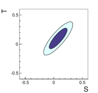
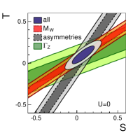
Figure 1: Two-dimensional probability distributions for the oblique parameters $S$ and $T$ at $68\%$ (the dark region) and $95\%$ (the light region) floating $U$ (left) or fixing $U=0$ (right). In the right plot, the individual constraints from $M_{W}$, the asymmetry parameters $\sin^{2}\theta_{\rm eff}^{\rm lept}$, $P_{\tau}^{\rm pol}$, $A_{f}$ and $A_{\rm FB}^{0,f}$ with $f=\ell,c,b$, and $\Gamma_{Z}$ are also presented.

Next we consider the epsilon parameters introduced in Refs [16, 17, 18]. Unlike the $S$, $T$, and $U$ parameters discussed above, the epsilon parameters involve SM contributions associated with the top quark and the Higgs boson. Moreover, they also involve flavour non-universal vertex corrections in the SM [6] and the vacuum-polarization corrections that are not taken into account in the $S$, $T$, and $U$ parameters [40]. Since all the SM parameters, including $m_{t}$ and $m_{H}$, have now been measured, we separate the NP contribution from the SM one, by defining,

$$\delta\epsilon_{i}=\epsilon_{i}-\epsilon_{i,\mathrm{SM}}\qquad\mathrm{for}\ \ i=1,2,3,b,$$ (1)

where $\epsilon_{i}$ are the original epsilon parameters. Here and in the following, a quantity with the subscript “SM” represents the corresponding SM contribution. Using $\delta\epsilon_{i}$, the $W$-boson mass and the effective vector and axial-vector couplings for the $Zf\bar{f}$ interactions are given by

$$M_{W} =M_{W,\mathrm{SM}}\Bigg{\{}1-\frac{1}{2(c_{W,\mathrm{SM}}^{2}-s_{W,\mathrm{SM}}^{2})}$$

$$\hskip 28.45274pt\times\Big{[}-c_{0}^{2}\delta\epsilon_{1}+(c_{0}^{2}-s_{0}^{2})\delta\epsilon_{2}+2s_{0}^{2}\delta\epsilon_{3}\Big{]}\Bigg{\}}\,,$$ (2)

$$g_{V}^{f} =g_{V,\mathrm{SM}}^{f}+\Big{(}g_{V,\mathrm{SM}}^{f}-g_{A,\mathrm{SM}}^{f}\Big{)}\Bigg{(}\frac{\delta\epsilon_{3}-c_{0}^{2}\,\delta\epsilon_{1}}{c_{0}^{2}-s_{0}^{2}}-\delta\epsilon_{b}\Bigg{)}$$

$$\hskip 14.22636pt+\frac{g_{V,\mathrm{SM}}^{f}}{2}\,\big{(}\delta\epsilon_{1}+2\delta\epsilon_{b}\big{)}\,,$$ (3)

$$g_{A}^{f} =g_{A,\mathrm{SM}}^{f}+\frac{I_{3}^{f}}{2}\big{(}\delta\epsilon_{1}+2\delta\epsilon_{b}\big{)}\,,$$ (4)

where $\delta\epsilon_{b}=0$ for $f\neq b$, $I_{3}^{f}$ is the third component of weak isospin of fermion $f$, and $s_{W}$, $c_{W}$, $s_{0}$ and $c_{0}$ are defined in Ref. [6]. Using the above effective couplings, the $Z$-pole observables are calculated with the formulae presented in Appendix A of Ref. [6]. Our fit results for the $\delta\epsilon_{i}$ parameters are summarized in Tables 4 and 5, where $\delta\epsilon_{2}$ and $\delta\epsilon_{b}$ are set to be zero in the latter. The corresponding two-dimensional probability distributions for $\delta\epsilon_{1}$ and $\delta\epsilon_{3}$ are plotted in Fig. 2. The results are consistent with the SM.

	Fit result	Correlations
$\delta\epsilon_{1}$	$\phantom{-}0.0007\pm 0.0010$	$1.00$
$\delta\epsilon_{2}$	$-0.0001\pm 0.0009$	$0.80$	$1.00$
$\delta\epsilon_{3}$	$\phantom{-}0.0006\pm 0.0009$	$0.86$	$0.51$	$1.00$
$\delta\epsilon_{b}$	$\phantom{-}0.0003\pm 0.0013$	$-0.33$	$-0.32$	$-0.22$	$1.00$

Table 4: Fit results for the $\delta\epsilon_{i}$ parameters.

	Fit result	Correlations
$\delta\epsilon_{1}$	$0.0008\pm 0.0006$	$1.00$
$\delta\epsilon_{3}$	$0.0007\pm 0.0008$	$0.87$	$1.00$

Table 5: Fit results for $\delta\epsilon_{1}$ and $\delta\epsilon_{3}$ fixing $\delta\epsilon_{2}=\delta\epsilon_{b}=0$.

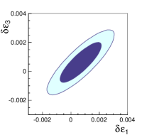
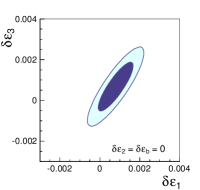
Figure 2: Two-dimensional probability distributions for $\delta\epsilon_{1}$ and $\delta\epsilon_{3}$ at $68\%$ (the dark region) and $95\%$ (the light region) floating all $\delta\epsilon_{i}$ parameters (left) or fixing $\delta\epsilon_{2}=\delta\epsilon_{b}=0$ (right).

	Fit result	Correlations
$\delta g_{R}^{b}$	$0.018\pm 0.007$	$1.00$
$\delta g_{L}^{b}$	$0.0029\pm 0.0014$	$0.90$	$1.00$
$\delta g_{V}^{b}$	$\phantom{-}0.021\pm 0.008$	$1.00$
$\delta g_{A}^{b}$	$-0.015\pm 0.006$	$-0.98$	$1.00$

Table 6: Fit results for the shifts in the $Zb\bar{b}$ couplings.

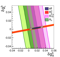
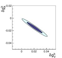
Figure 3: Two-dimensional probability distributions for $\delta g_{R}^{b}$ and $\delta g_{L}^{b}$ (left), or $\delta g_{V}^{b}$ and $\delta g_{A}^{b}$ (right) at $68\%$ (the dark region) and $95\%$ (the light region). The individual constraints in the left plot are computed by omitting $\mathcal{A}_{b}$, $A_{\rm FB}^{0,b}$, $\Gamma_{Z}$, $\sigma_{h}^{0}$, $R_{\ell}^{0}$, $R_{c}^{0}$ and $R_{b}^{0}$ except when specified in the legend.

We also consider the case where dominant NP contributions appear in the $Zb\bar{b}$ couplings (see, e.g., Ref. [41] and references therein). We parameterize NP contributions to the $Zb\bar{b}$ couplings as follows:

$$g_{i}^{b} =g^{b}_{i,\mathrm{SM}}+\delta g_{i}^{b}\qquad\mathrm{for}\ \ i=R,L,V,A,$$ (5)

where the definitions of these couplings are given in Ref. [6]. The EW precision fit provides four solutions for the couplings, while two of them are disfavored by the off $Z$-pole data for the forward-backward asymmetry in $e^{+}e^{-}\to b\bar{b}$ [42]. In Tables 6 and Fig. 3, we present the solution that is closer to the SM. We observe significant deviations from the SM, which are attributed to the measured value of $A_{\mathrm{FB}}^{0,b}$.

In various NP models the Higgs-boson couplings to the SM vector bosons and fermions deviate from their SM values. It is therefore of interest to study constraints on the Higgs-boson couplings from the EW precision test. We consider a general effective Lagrangian for a light Higgs-boson-like scalar field $H$, assuming an approximate custodial symmetry and no other new light states below a cutoff scale [43, 44, 45, 46]:

$$\mathcal{L}=\frac{v^{2}}{4}{\rm Tr}\big{(}D_{\mu}\Sigma^{\dagger}D^{\mu}\Sigma\big{)}\left(1+2\kappa_{V}\frac{H}{v}+\cdots\right)+\cdots,$$ (6)

where $v$ is the vacuum expectation value of the Higgs-boson field, and the longitudinal components of the $W$ and $Z$ bosons, $\chi^{a}(x)$, are described by the two-by-two matrix $\Sigma(x)=\exp(i\tau^{a}\chi^{a}(x)/v)$ with $\tau^{a}$ being the Pauli matrices. The deviation in the $HVV$ couplings is parameterized by the scale factor $\kappa_{V}$, which is equal to one in the SM. The oblique parameters $S$ and $T$ then receive the following contributions [47]:

$$S =\frac{1}{12\pi}(1-\kappa_{V}^{2})\ln\bigg{(}\frac{\Lambda^{2}}{m_{H}^{2}}\bigg{)}\,,$$ (7)

$$T =-\frac{3}{16\pi c_{W}^{2}}(1-\kappa_{V}^{2})\ln\bigg{(}\frac{\Lambda^{2}}{m_{H}^{2}}\bigg{)}\,,$$ (8)

where $\Lambda=4\pi v/\sqrt{|1-\kappa_{V}^{2}|}$ is the cutoff scale of the effective Lagrangian. We present fit results for $\kappa_{V}$ in Table 7 and Fig. 4. Typical NP models, such as composite Higgs models, generate smaller $\kappa_{V}$ ($\kappa_{V}<1$), while larger $\kappa_{V}$ requires that the $W_{L}W_{L}$ scattering is dominated by an isospin-two channel [48, 49]. The present fit disfavors smaller $\kappa_{V}$, where the lower bound at 95% corresponds to the cutoff scale $\Lambda=18$ TeV. In the right plot of Fig. 4, we generalize the analysis allowing for $\Lambda<4\pi v/\sqrt{|1-\kappa_{V}^{2}|}$ and assuming that the dynamics at the cutoff does not contribute sizably to the oblique parameters. We find that $\kappa_{V}$ is tightly constrained for $\Lambda>1$ TeV. Extra contributions to the oblique parameters were studied, e.g., in Refs. [50, 51, 52, 53].

	68%	95%
$\kappa_{V}$	$1.025\pm 0.021$	$[0.985,\,1.069]$

Table 7: Fit results for the scale factor $\kappa_{V}$ at 68% and 95% probabilities.

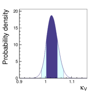
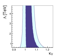
Figure 4: Left: Probability distribution for the scale factor $\kappa_{V}$. Right: Two-dimensional probability distributions for $\kappa_{V}$ and $\Lambda$. The dark and light regions correspond to $68\%$ and $95\%$ probabilities, respectively.

4 Constraints on the Higgs-boson couplings from the Higgs-boson and electroweak precision data

In this section we fit the Higgs-boson couplings to the data for the Higgs-boson signal strengths and the EWPO, where the former are taken from Refs. [31, 54] for $H\to\gamma\gamma$, Refs. [55, 56] for $H\to ZZ$, Refs. [57, 58] for $H\to W^{+}W^{-}$, Refs. [59, 60] for $H\to\tau^{+}\tau^{-}$, and Refs. [61, 62, 63, 64, 65] for $H\to b\bar{b}$ (see also Ref. [66]). We consider the scale factors $\kappa_{V}$ and $\kappa_{f}$ for the Higgs-boson couplings to the EW vector bosons and to fermions, respectively, and do not introduce new couplings that are absent in the SM. For the SM loop-induced couplings ($Hgg$, $H\gamma\gamma$, and $HZ\gamma$) we assume that there is no contribution from new particles in the loop. For the relations between the scale factors and the Higgs-boson signal strengths, we refer the reader to Ref. [67].

	68%	95%	Correlations
$\kappa_{V}$	$1.02\pm 0.05$	$[0.93,\,1.11]$	$1.00$
$\kappa_{f}$	$0.97\pm 0.11$	$[0.76,\,1.20]$	$0.22$	$1.00$

Table 8: SM-like solution in the fit of $\kappa_{V}$ and $\kappa_{f}$ to the Higgs-boson signal strengths.

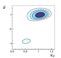
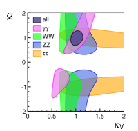
Figure 5: Left: Two-dimensional probability distributions for $\kappa_{V}$ and $\kappa_{f}$ at 68%, 95%, 99%, and 99.9% (darker to lighter), obtained from the fit to the Higgs-boson signal strengths. Right: Constraints from individual channels at 95%.

	68%	95%	Correlations
$\kappa_{V}$	$1.02\pm 0.02$	$[0.99,\,1.06]$	$1.00$
$\kappa_{f}$	$0.97\pm 0.11$	$[0.77,\,1.20]$	$0.10$	$1.00$

Table 9: Same as Table 8, but considering both the Higgs-boson signal strengths and the EWPO.

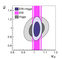
Figure 6: Two-dimensional probability distributions for $\kappa_{V}$ and $\kappa_{f}$ at $68\%$ (the dark region) and $95\%$ (the light region), obtained from the fit to the Higgs-boson signal strengths and the EWPO.

In Table 8 we summarize the fit results for $\kappa_{V}$ and $\kappa_{f}$ from the Higgs-boson signal strengths. Note that theoretical predictions are symmetric under the exchange $\{\kappa_{V},\ \kappa_{f}\}\leftrightarrow\{-\kappa_{V},\ -\kappa_{f}\}$. In the left plot in Fig. 5, we present two-dimensional probability distributions for $\kappa_{V}$ and $\kappa_{f}$ at 68%, 95%, 99%, and 99.9%, where only the parameter space with positive $\kappa_{V}$ is presented. The region with negative $\kappa_{f}$ is disfavored in the fit. The right plot in Fig. 5 shows constraints from the individual decay channels. The constraints from $H\to b\bar{b}$ are weaker than that from $H\to\tau^{+}\tau^{-}$ and are not presented for simplicity. It is noted that because of the presence of flat directions in the fit, the detailed shapes of the individual constraints depend on the choice of the allowed ranges of the scale factors. We also consider constraints from the EWPO with the formulae in Eqs. (7) and (8), which are valid under the assumptions given above Eq. (6). As shown in Table 9 and Fig. 6, the constraint on $\kappa_{V}$ from the EWPO is stronger than that from the Higgs-boson signal strengths.

Next we consider the case where the coupling to $W^{+}W^{-}$, parameterized by $\kappa_{W}$, can differ from that to $ZZ$, parameterized by $\kappa_{Z}$. Note that theoretical predictions are symmetric under the exchanges $\{\kappa_{W},\ \kappa_{f}\}\leftrightarrow\{-\kappa_{W},\ -\kappa_{f}\}$ and/or $\kappa_{Z}\leftrightarrow-\kappa_{Z}$, where $\kappa_{Z}$ can flip the sign independent of $\kappa_{W}$, since the interference between the $W$ and $Z$ contributions to the vector-boson fusion cross section is negligible. Hence we consider only the parameter space where both $\kappa_{W}$ and $\kappa_{Z}$ are positive. Here we do not consider the EWPO, since $\kappa_{W}\neq\kappa_{Z}$ develops power divergences in the oblique corrections. It means that the detailed information on UV theory is necessary for calculating the oblique corrections. The fit results to the Higgs-boson signal strengths are summarized in Table 10 and Fig. 7, which are consistent with custodial symmetry.

	68%	95%	Correlations
$\kappa_{W}$	$1.00\pm 0.06$	$[0.88,\,1.11]$	$1.00$
$\kappa_{Z}$	$1.09\pm 0.10$	$[0.88,\,1.27]$	$-0.12$	$1.00$
$\kappa_{f}$	$0.94\pm 0.12$	$[0.72,\,1.18]$	$0.35$	$-0.16$	$1.00$

Table 10: SM-like solution in the fit of $\kappa_{W}$, $\kappa_{Z}$, and $\kappa_{f}$ to the Higgs-boson signal strengths.

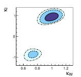
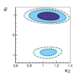
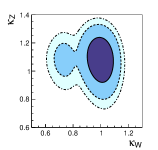
Figure 7: Two-dimensional probability distributions for $\kappa_{W}$ and $\kappa_{f}$ (left), for $\kappa_{Z}$ and $\kappa_{f}$ (center), and for $\kappa_{W}$ and $\kappa_{Z}$ (right) at $68\%$, $95\%$, and $99\%$ (darker to lighter), obtained from the fit to the Higgs-boson signal strengths.

We also consider the case where the universality in the couplings to the fermions is relaxed by introducing $\kappa_{\ell}$, $\kappa_{u}$ and $\kappa_{d}$ for the couplings to the charged leptons, to the up-type quarks, and to the down-type quarks. In this case, the Higgs-boson signal strengths are symmetric under the exchanges $\kappa_{\ell}\leftrightarrow-\kappa_{\ell}$ and/or $\{\kappa_{V},\ \kappa_{u},\ \kappa_{d}\}\leftrightarrow\{-\kappa_{V},\ -\kappa_{u},\ -\kappa_{d}\}$. Therefore, we consider only the parameter space where both $\kappa_{V}$ and $\kappa_{\ell}$ are positive. The constraints on the scale factors from the Higgs-boson signal strengths are presented in Table 11 and Fig. 8. By adding the EWPO to the fit, the constraints become stronger as shown in Table 12 and Fig. 9.

	68%	95%	Correlations
$\kappa_{V}$	$1.07\pm 0.09$	$[0.87,\,1.24]$	$1.00$
$\kappa_{\ell}$	$1.13\pm 0.17$	$[0.80,\,1.47]$	$0.54$	$1.00$
$\kappa_{u}$	$0.89\pm 0.13$	$[0.65,\,1.18]$	$0.37$	$0.36$	$1.00$
$\kappa_{d}$	$1.01\pm 0.24$	$[0.52,\,1.51]$	$0.79$	$0.60$	$0.75$	$1.00$

Table 11: SM-like solution in the fit of $\kappa_{V}$, $\kappa_{\ell}$, $\kappa_{u}$, and $\kappa_{d}$ to the Higgs-boson signal strengths.

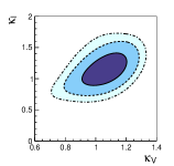
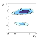
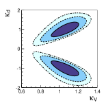
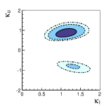
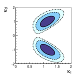
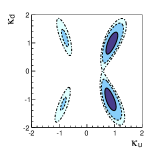
Figure 8: Two-dimensional probability distributions for $\kappa_{V}$ and $\kappa_{\ell}$ (top-left), for $\kappa_{V}$ and $\kappa_{u}$ (top-center), for $\kappa_{V}$ and $\kappa_{d}$ (top-right), for $\kappa_{\ell}$ and $\kappa_{u}$ (bottom-left), for $\kappa_{\ell}$ and $\kappa_{d}$ (bottom-center), and for $\kappa_{u}$ and $\kappa_{d}$ (bottom-right) at $68\%$, $95\%$, and $99\%$ (darker to lighter), obtained from the fit to the Higgs-boson signal strengths.

	68%	95%	Correlations
$\kappa_{V}$	$1.03\pm 0.02$	$[0.99,\,1.07]$	$1.00$
$\kappa_{\ell}$	$1.10\pm 0.14$	$[0.82,\,1.38]$	$0.14$	$1.00$
$\kappa_{u}$	$0.88\pm 0.12$	$[0.66,\,1.15]$	$0.09$	$0.23$	$1.00$
$\kappa_{d}$	$0.92\pm 0.15$	$[0.65,\,1.26]$	$0.28$	$0.35$	$0.81$	$1.00$

Table 12: Same as Table 11, but considering both the Higgs-boson signal strengths and the EWPO.

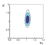
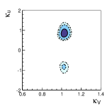
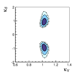
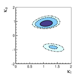
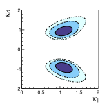
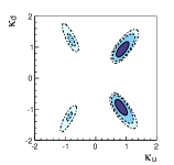
Figure 9: Same as Fig. 8, but considering both the Higgs-boson signal strengths and the EWPO.

5 Summary

We have updated the EW precision fits in the SM and beyond taking into account the recent theoretical and experimental developments. The results of the SM fit are presented in Table 1, while the constraints on the NP parameters (the oblique and epsilon parameters, and the modified $Zb\bar{b}$ and $HVV$ couplings) are summarized in Tables 2-7. Furthermore, we have performed fits of the scale factors of the Higgs-boson couplings to the Higgs-boson signal strengths and the EW precision data as summarized in Tables 8-12. More detailed analyses and results will be presented in a future publication [68].

References

- [1] The ATLAS collaboration, G. Aad, et al., Phys.Lett. B716 (2012) 1. arXiv:1207.7214.
- [2] The CMS collaboration, S. Chatrchyan, et al., Phys.Lett. B716 (2012) 30. arXiv:1207.7235.
- [3] O. Eberhardt, et al., Phys.Rev.Lett. 109 (2012) 241802. arXiv:1209.1101.
- [4] The Gfitter group, M. Baak, et al., Eur.Phys.J. C72 (2012) 2205. arXiv:1209.2716.
- [5] J. Erler, arXiv:1209.3324.
- [6] M. Ciuchini, E. Franco, S. Mishima, L. Silvestrini, JHEP 1308 (2013) 106. arXiv:1306.4644.
- [7] J. de Blas, EPJ Web Conf. 60 (2013) 19008. arXiv:1307.6173.
- [8] The Gfitter group, M. Baak, et al., Eur.Phys.J. C74 (2014) 3046. arXiv:1407.3792.
- [9] A. Freitas, Y.-C. Huang, JHEP 1208 (2012) 050. arXiv:1205.0299.
- [10] A. Freitas, Phys.Lett. B730 (2014) 50. arXiv:1310.2256.
- [11] A. Freitas, JHEP 1404 (2014) 070. arXiv:1401.2447.
- [12] A. Freitas, arXiv:1406.6980.
- [13] A. Caldwell, D. Kollar, K. Kroninger, Comput.Phys.Commun. 180 (2009) 2197. arXiv:0808.2552.
- [14] M. E. Peskin, T. Takeuchi, Phys.Rev.Lett. 65 (1990) 964.
- [15] M. E. Peskin, T. Takeuchi, Phys.Rev. D46 (1992) 381.
- [16] G. Altarelli, R. Barbieri, Phys.Lett. B253 (1991) 161.
- [17] G. Altarelli, R. Barbieri, S. Jadach, Nucl.Phys. B369 (1992) 3.
- [18] G. Altarelli, R. Barbieri, F. Caravaglios, Nucl.Phys. B405 (1993) 3.
- [19] The UTfit collaboration, M. Bona, et al., JHEP 0507 (2005) 028. arXiv:hep-ph/0501199.
- [20] The CMS collaboration, S. Chatrchyan, et al., Phys.Rev. D84 (2011) 112002. arXiv:1110.2682.
- [21] The ATLAS collaboration, ATLAS-CONF-2013-043 (2013).
- [22] The CDF collaboration, T. Aaltonen, et al., Phys.Rev. D88 (2013) 072002. arXiv:1307.0770.
- [23] The CDF collaboration, T. Aaltonen, et al., Phys.Rev. D89 (2014) 072005. arXiv:1402.2239.
- [24] The D0 collaboration, V. M. Abazov, et al., arXiv:1408.5016.
- [25] The Particle Data Group, J. Beringer, et al., Phys.Rev. D86 (2012) 010001, and 2013 partial update for the 2014 edition.
- [26] The ATLAS, CDF, CMS and D0 collaborations, arXiv:1403.4427.
- [27] The CMS collaboration, CMS-PAS-TOP-14-001 (2014).
- [28] The D0 collaboration, V. M. Abazov, et al., Phys.Rev.Lett. 113 (2014) 032002. arXiv:1405.1756.
- [29] The Tevatron Electroweak Working Group, arXiv:1407.2682.
- [30] The ATLAS collaboration, G. Aad, et al., Phys.Rev. D90 (2014) 052004. arXiv:1406.3827.
- [31] The CMS collaboration, CMS-PAS-HIG-13-001 (2013).
- [32] The CMS collaboration, S. Chatrchyan, et al., Phys.Rev. D89 (2014) 092007. arXiv:1312.5353.
- [33] P. Z. Skands, D. Wicke, Eur.Phys.J. C52 (2007) 133. arXiv:hep-ph/0703081.
- [34] D. Wicke, P. Z. Skands, Nuovo Cim. B123 (2008) S1. arXiv:0807.3248.
- [35] A. Buckley, et al., Phys.Rept. 504 (2011) 145. arXiv:1101.2599.
- [36] M. Mangano, talk given at TOP2013, Durbach, Germany, Sep. 14-19, 2013.
- [37] S. Moch, et al., arXiv:1405.4781.
- [38] S. Moch, arXiv:1408.6080.
- [39] M. Davier, A. Hoecker, B. Malaescu, Z. Zhang, Eur.Phys.J. C71 (2011) 1515. arXiv:1010.4180.
- [40] R. Barbieri, A. Pomarol, R. Rattazzi, A. Strumia, Nucl.Phys. B703 (2004) 127. arXiv:hep-ph/0405040.
- [41] B. Batell, S. Gori, L.-T. Wang, JHEP 1301 (2013) 139. arXiv:1209.6382.
- [42] D. Choudhury, T. M. Tait, C. Wagner, Phys.Rev. D65 (2002) 053002. arXiv:hep-ph/0109097.
- [43] G. Giudice, C. Grojean, A. Pomarol, R. Rattazzi, JHEP 0706 (2007) 045. arXiv:hep-ph/0703164.
- [44] R. Contino, et al., JHEP 1005 (2010) 089. arXiv:1002.1011.
- [45] A. Azatov, R. Contino, J. Galloway, JHEP 1204 (2012) 127. arXiv:1202.3415.
- [46] R. Contino, et al., JHEP 1307 (2013) 035. arXiv:1303.3876.
- [47] R. Barbieri, B. Bellazzini, V. S. Rychkov, A. Varagnolo, Phys.Rev. D76 (2007) 115008. arXiv:0706.0432.
- [48] A. Falkowski, S. Rychkov, A. Urbano, JHEP 1204 (2012) 073. arXiv:1202.1532.
- [49] B. Bellazzini, L. Martucci, R. Torre, JHEP 1409 (2014) 100. arXiv:1405.2960.
- [50] C. Grojean, W. Skiba, J. Terning, Phys.Rev. D73 (2006) 075008. arXiv:hep-ph/0602154.
- [51] A. Azatov, R. Contino, A. Di Iura, J. Galloway, Phys.Rev. D88 (2013) 075019. arXiv:1308.2676.
- [52] A. Pich, I. Rosell, J. J. Sanz-Cillero, Phys.Rev.Lett. 110 (2013) 181801. arXiv:1212.6769.
- [53] A. Pich, I. Rosell, J. J. Sanz-Cillero, JHEP 1401 (2014) 157. arXiv:1310.3121.
- [54] The ATLAS collaboration, ATLAS-CONF-2013-012 (2013).
- [55] The ATLAS collaboration, ATLAS-CONF-2013-013 (2013).
- [56] The CMS collaboration, CMS-PAS-HIG-13-002 (2013).
- [57] The ATLAS collaboration, ATLAS-CONF-2013-030 (2013).
- [58] The CMS collaboration, S. Chatrchyan, et al., JHEP 1401 (2014) 096. arXiv:1312.1129.
- [59] The ATLAS collaboration, ATLAS-CONF-2013-108 (2013).
- [60] The CMS collaboration, CMS-PAS-HIG-13-004 (2013).
- [61] The CDF and D0 collaborations, arXiv:1207.0449.
- [62] The ATLAS collaboration, ATLAS-CONF-2013-079 (2013).
- [63] The ATLAS collaboration, ATLAS-CONF-2014-011 (2014).
- [64] The CMS collaboration, S. Chatrchyan, et al., Phys.Rev. D89 (2014) 012003. arXiv:1310.3687.
- [65] The CMS collaboration, CMS-PAS-HIG-13-019 (2013).
- [66] P. Bechtle, et al., arXiv:1403.1582.
- [67] LHC Higgs Cross Section Working Group, S. Heinemeyer, et al. (Eds.), CERN-2013-004 (2013). arXiv:1307.1347.
- [68] M. Ciuchini, E. Franco, S. Mishima, M. Pierini, L. Reina, L. Silvestrini, in preparation.