Homogenization of a system of elastic and reaction-diffusion equations modelling plant cell wall biomechanics

Abstract.

In this paper we present a derivation and multiscale analysis of a mathematical model for plant cell wall biomechanics that takes into account both the microscopic structure of a cell wall coming from the cellulose microfibrils and the chemical reactions between the cell wall’s constituents. Particular attention is paid to the role of pectin and the impact of calcium-pectin cross-linking chemistry on the mechanical properties of the cell wall. We prove the existence and uniqueness of the strongly coupled microscopic problem consisting of the equations of linear elasticity and a system of reaction-diffusion and ordinary differential equations. Using homogenization techniques (two-scale convergence and periodic unfolding methods) we derive a macroscopic model for plant cell wall biomechanics.

Key words: Homogenization; two-scale convergence; periodic unfolding method; elasticity; reaction-diffusion equations; plant modelling.

AMS subject classifications: 35B27, 35Q92, 35Kxx, 74Qxx, 74A40, 74D05

Introduction

For a better understanding of plant growth and development it is important to analyse the influence of chemical processes on the mechanical properties (elasticity and extensibility) of plant cells. The main feature of plant cells are their walls, which must be strong to resist a high internal hydrostatic pressure (turgor pressure) and flexible to permit growth. Plant cell walls consist of a wall matrix (composed mainly of pectin, hemicellulose, structural proteins, and water) and cellulose microfibrils. It is supposed that calcium-pectin cross-linking chemistry is one of the main regulators of plant cell wall elasticity and extension [61]. Pectin is deposited into cell walls in a methylesterified form. In cell walls pectin can be modified by the enzyme pectin methylesterase (PME), which removes methyl groups by breaking ester bonds. The de-esterified pectin is able to form calcium-pectin cross-links, and so stiffen the cell wall and reduce its expansion. On the other hand, mechanical stresses can break calcium-pectin cross-links and hence increase the extensibility of plant cell walls.

To analyse the interactions between calcium-pectin dynamics and the deformations of a plant cell wall, as well as the influence of the microscopic structure on the mechanical properties of a cell wall, we derive a mathematical model for plant cell wall biomechanics at the length scale of cell wall microfibrils. We model the cell wall as a three-dimensional continuum consisting of a wall matrix and microfibrils. Within the wall matrix, we consider the dynamics of five chemical substances: the enzyme PME, methylesterfied pectin, demethylesterfied pectin, calcium ions, and calcium-pectin cross-links. The cell wall matrix is assumed to be isotropic and linearly elastic, whereas microfibrils are modelled as an anisotropic, linearly elastic material. The interplay between the mechanics and the cross-link dynamics comes in by assuming that the elastic properties of the matrix depend on the density of the cross-links and that strain or stress within the cell wall can break calcium-pectin cross-links. The strain- or stress-dependent opening of calcium channels in the cell plasma membrane is addressed in the flux boundary conditions for calcium ions. We consider two different cases, one in which the calcium-pectin cross-links diffuse and another in which they do not diffuse. Thus the microscopic problem is a strongly coupled system of reaction-diffusion equations or reaction-diffusion and ordinary differential equations, with reaction terms depending on the displacement gradient, and the equations of linear elasticity, with elastic moduli depending on the density of calcium-pectin cross-links.

To analyse the macroscopic behaviour of plant cell walls, comprising a complex microscopic structure, we rigorously derive a macroscopic model for plant cell wall biomechanics. As there are thousands of microfibrils in a plant cell wall, the derivation of the macroscopic equations is also important for effective numerical simulations. The two-scale convergence, e.g. [3, 42], and the periodic unfolding method, e.g. [11, 12], are applied to obtain the macroscopic equations. Some previous results on the homogenization of problems in linear elasticity can be found in [4, 5, 28, 43, 53] (and the references therein). A multiscale analysis of microscopic problems comprising the equations of linear elasticity for a solid matrix or cells combined with the Stokes equations for the fluid part was considered in [23, 27, 39].

The main novelty of this paper is twofold: (i) we derive a new model for plant cell wall biomechanics where the mechanical properties and biochemical processes in a cell wall are considered on the scale of its structural elements (on the scale of the microfibrils) and (ii) using homogenization techniques we obtain a macroscopic model for plant cell wall biomechanics from a microscopic description of the mechanical and chemical processes. This approach allows us to take into account the complex microscopic structure of a plant cell wall and to analyze the impact of the heterogeneous distribution of cell wall’s structural elements on the mechanical properties and development of plants.

The main mathematical difficulty arises from the strong coupling between the equations of linear elasticity for cell wall mechanics and the system of reaction-diffusion and ordinary differential equations for the chemical processes in the wall matrix. The Galerkin method together with classical fixed-point approaches are used to prove the existence of a unique solution of the microscopic problem. However, since the reaction terms depend on the displacement gradient and the elasticity tensor is a function of the density of chemical substances, the derivation of a contraction inequality is non-standard and relies on estimates for the $L^{\infty}$-norm of the solutions of the reaction-diffusion and ordinary differential equations in term of the $L^{2}$-norm of the displacement gradient. The theory of positively invariant regions [51, 55] and the Alikakos [2] iteration techniques are applied to show the non-negativity and uniform boundedness of solutions of the microscopic model. The iteration technique [2] is also used to derive a contraction inequality.

The analysis of the coupled system also depends strongly on the microscopic model for the chemical processes. For the chemical processes in the cell wall matrix we consider two situations: (i) chemical processes are described by a system of reaction-diffusion and ordinary differential equations and (ii) all chemical processes are modelled by reaction-diffusion equations.

In the first situation, the solutions of the ordinary differential equation have the same regularity with respect to the spatial variables as the reaction terms. Thus, for the proof of the well-posedness results for the microscopic problem and for the rigorous derivation of the macroscopic equations, the dependence of the reaction terms on a local average of the displacement gradient is essential. The well-posedness of the microscopic problem can be proven by considering an $\varepsilon$-average, where the small parameter $\varepsilon$ characterizes the microscopic structure of the cell wall. However, the proof of the strong convergence for a sequence of solutions of the ordinary differential equation, which is necessary for the homogenization of the microscopic problem, relies on the fact that the local average is independent of $\varepsilon$. Also, in the proof of the strong convergence we apply the unfolding operator to map solutions of the ordinary differential equation, defined in a perforated $\varepsilon$-dependent domain, to a fixed domain.

In the second case when all chemical substances diffuse, solutions of the reaction-diffusion equations have higher regularity with respect to the spatial variables and a point-wise dependence of the reaction terms on the displacement gradient can be considered. In this situation in order to pass to the limit in the nonlinear reaction terms we prove the strong two-scale convergence for the displacement gradient.

Similar to the microscopic problems, the uniqueness of a solution of the macroscopic equations is proven by deriving a contraction inequality involving the $L^{\infty}$-norm of the difference of two solutions of the reaction-diffusion and ordinary differential equations.

The paper is organised as follows. In Section 1 we give the general setting of the two microscopic models for plant cell wall biomechanics. The main results of the paper are summarized in Section 2. The existence and uniqueness results for weak solutions of the two microscopic problems are proven in Sections 3 and 4. The homogenization and derivation of the macroscopic equations for both microscopic models for plant cell wall biomechanics are conducted in Sections 5 and 6. Some results on the numerical simulations of the unit cell problems, which determine the effective macroscopic elastic properties of a plant cell wall, are given in Section 8. The detailed derivation of the microscopic model for plant cell wall biomechanics on the length-scale of the cell wall microfibrils is presented in Section 9. Concluding remarks are included in Section 10.

1. Formulation of the mathematical models for plant cell wall biomechanics.

In the mathematical model for plant cell wall biomechanics we consider interactions between the mechanical properties of the plant cell wall and the chemical processes in the cell wall. The derivation of the models is presented in Section 9.

In the mathematical model we consider the microscopic structure of a plant cell wall, which is given by microfibrils embedded in the cell wall matrix. By $\Omega\subset\mathbb{R}^{3}$ we denote a domain occupied by a flat section of a plant cell wall and can consider $\Omega=(0,a_{1})\times(0,a_{2})\times(0,a_{3})$, where $a_{i}$, $i=1,2,3$, are positive numbers. We assume that the microfibrils are oriented in the $x_{3}$-direction, see Fig. 1(a). The part of $\partial\Omega$ on the exterior of the cell wall is given by $\Gamma_{{\mathcal{E}}}=\{a_{1}\}\times(0,a_{2})\times(0,a_{3}),$ and the interior boundary $\Gamma_{\mathcal{I}}$ of the cell wall is given by $\Gamma_{{\mathcal{I}}}=\{0\}\times(0,a_{2})\times(0,a_{3}).$ The top and bottom boundaries are defined by $\Gamma_{\mathcal{U}}=(0,a_{1})\times\{0\}\times(0,a_{3})\cup(0,a_{1})\times\{a_{2}\}\times(0,a_{3})$.

To determine the microscopic structure of the cell wall, we consider $\hat{Y}=(0,1)^{2}$ and an open subset $\hat{Y}_{F}$, with $\overline{\hat{Y}_{F}}\subset\hat{Y}$, and define $\hat{Y}_{M}=\hat{Y}\setminus\overline{\hat{Y}_{F}}$, $Y=\hat{Y}\times(0,a_{3})$, $Y_{F}=\hat{Y}_{F}\times(0,a_{3})$, and $Y_{M}=Y\setminus\overline{Y_{F}}$, where $Y_{M}$ and $Y_{F}$ represent the cell wall matrix and a microfibril, respectivelly, see Fig. 1(b). We also denote $\Gamma=\partial Y_{F}$ and $\hat{\Gamma}=\partial\hat{Y}_{F}$.

We assume that the microfibrils in the cell wall are distributed periodically and have a diameter on the order of $\varepsilon$, where the small parameter $\varepsilon$ characterizes the size of the microstructure (the ratio of the diameter of microfibrils to the thickness of the cell wall, i.e.  the microfibrils of a plant cell wall are about $3$ nm in diameter and are separated by a distance of about $6$ nm, see e.g. [14, 29, 57], whereas the thickness of a plant cell wall is of the order of a few micrometers). The domains

$$\Omega_{F}^{\varepsilon}=\bigcup_{\xi\in\mathbb{Z}^{2}}\big{\{}\varepsilon(\hat{Y}_{F}+\xi)\times(0,a_{3})\;\;|\;\;\varepsilon(\hat{Y}+\xi)\subset(0,a_{1})\times(0,a_{2})\big{\}}\qquad\text{ and }\qquad\Omega_{M}^{\varepsilon}=\Omega\,\setminus\overline{\Omega_{F}^{\varepsilon}}$$

denote the part of $\Omega$ occupied by the microfibrils and by the cell wall matrix, respectively. The boundary between the matrix and the microfibrils is denoted by

$$\Gamma^{\varepsilon}=\partial\Omega_{M}^{\varepsilon}\cap\partial\Omega_{F}^{\varepsilon}.$$

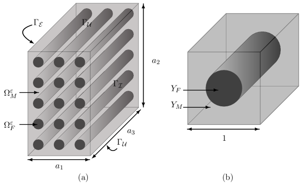
Figure 1. (a) A depiction of the domain $\Omega$ with the subsets representing the cell wall matrix $\Omega_{M}^{\varepsilon}$ and the microfibrils $\Omega_{F}^{\varepsilon}$. The surface $\Gamma_{\mathcal{I}}$ is in contact with the interior of the cell, and the (hidden) surface $\Gamma_{\mathcal{E}}$ is facing the outside of the cell, and $\Gamma_{\mathcal{U}}$ is the union of the surfaces on the top and bottom of $\Omega$. (b) A depiction of the unit cell $Y$.

In the mathematical model of plant cell wall biomechanics we consider deformations of the cell wall and the interactions between five species within the plant cell wall matrix: the number densities of methylestrified pectin $\textbf{p}_{1}^{\varepsilon}$, of enzyme PME $\textbf{p}_{2}^{\varepsilon}$, of demethylestrified pectin $\textbf{n}_{1}^{\varepsilon}$, of calcium ions $\textbf{n}_{2}^{\varepsilon}$, and of calcium-pectin cross-links $b^{\varepsilon}$. We shall consider two situations: (i) it is assumed that the calcium-pectin cross-links $b^{\varepsilon}$ do not diffuse and (ii) the diffusion of the calcium-pectin cross-links $b^{\varepsilon}$ in the cell wall matrix is considered.

Model I: In the first case, where the calcium-pectin cross-links $b^{\varepsilon}$ do not diffuse, the microscopic problem is composed of a system of reaction-diffusion and ordinary differential equations for $\textbf{p}^{\varepsilon}=(\textbf{p}^{\varepsilon}_{1},\textbf{p}^{\varepsilon}_{2})^{T}$, $\textbf{n}^{\varepsilon}=(\textbf{n}^{\varepsilon}_{1},\textbf{n}^{\varepsilon}_{2})^{T}$, and $b^{\varepsilon}$, coupled with the equations of linear elasticity for the displacement ${\bf u}^{\varepsilon}$

(2) $$\partial_{t}{\bf p}^{\varepsilon}=\text{div}(D_{p}\nabla\textbf{p}^{\varepsilon})-\textbf{F}_{p}(\textbf{p}^{\varepsilon})\hskip 167.87108pt\text{in}\ (0,T)\times\Omega^{\varepsilon}_{M},$$

$$\begin{aligned} &\partial_{t}\textbf{n}^{\varepsilon}=\text{div}(D_{n}\nabla\textbf{n}^{\varepsilon})+\textbf{F}_{n}(\textbf{p}^{\varepsilon},\textbf{n}^{\varepsilon})+\textbf{R}_{n}(\textbf{n}^{\varepsilon},b^{\varepsilon},\mathcal{N}_{\delta}({\bf e}({\bf u}^{\varepsilon})))\quad\\ &\partial_{t}b^{\varepsilon}=\phantom{\text{div}(D_{c}\nabla n^{\varepsilon})++\textbf{F}_{n}(\textbf{p}^{\varepsilon},\textbf{n}^{\varepsilon})\quad}R_{b}(\textbf{n}^{\varepsilon},b^{\varepsilon},\mathcal{N}_{\delta}({\bf e}({\bf u}^{\varepsilon})))\end{aligned}\qquad\text{in}\ (0,T)\times\Omega^{\varepsilon}_{M},$$

with the boundary and initial conditions

(3) $$\begin{cases}D_{p}\nabla\textbf{p}^{\varepsilon}\,\boldsymbol{\nu}=\textbf{J}_{p}(\textbf{p}^{\varepsilon})\\ D_{n}\nabla\textbf{n}^{\varepsilon}\,\boldsymbol{\nu}=\textbf{G}(\textbf{n}^{\varepsilon})\,\mathcal{N}_{\delta}({\bf e}({\bf u}^{\varepsilon}))\end{cases}\qquad \text{on}\ (0,T)\times\Gamma_{\mathcal{I}},$$

$$\begin{cases}D_{p}\nabla\textbf{p}^{\varepsilon}\,\boldsymbol{\nu}=-\gamma_{p}\,\textbf{p}^{\varepsilon}\qquad\\ D_{n}\nabla\textbf{n}^{\varepsilon}\,\boldsymbol{\nu}=\textbf{J}_{n}(\textbf{n}^{\varepsilon})\end{cases} \text{on}\ (0,T)\times\Gamma_{\mathcal{E}},$$

$$\;D_{p}\nabla\textbf{p}^{\varepsilon}\,\boldsymbol{\nu}=0,\;\;\quad D_{n}\nabla\textbf{n}^{\varepsilon}\,\boldsymbol{\nu}=0\qquad \text{on}\ (0,T)\times(\Gamma_{\mathcal{U}}\cup\Gamma^{\varepsilon}),$$

$$\;\textbf{p}^{\varepsilon},\;\textbf{n}^{\varepsilon} \quad\text{$a_{3}$-periodic in }x_{3},$$

$$\textbf{p}^{\varepsilon}(0,x)=\textbf{p}_{0}(x),\quad\textbf{n}^{\varepsilon}(0,x)=\textbf{n}_{0}(x),\quad b^{\varepsilon}(0,x)=b_{0}(x)\qquad \text{ for }\quad x\in\Omega_{M}^{\varepsilon},$$

where $\text{div}(D_{p}\nabla\textbf{p}^{\varepsilon})=(\text{div}(D_{p}^{1}\nabla\textbf{p}^{\varepsilon}_{1}),\text{div}(D_{p}^{2}\nabla\textbf{p}^{\varepsilon}_{2}))^{T}$ and $\text{div}(D_{n}\nabla\textbf{n}^{\varepsilon})=(\text{div}(D_{n}^{1}\nabla\textbf{n}^{\varepsilon}_{1}),\text{div}(D_{n}^{2}\nabla\textbf{n}^{\varepsilon}_{2}))^{T}$.

The displacement ${\bf u}^{\varepsilon}$ satisfies the equations of linear elasticity

(4) $$\left\{\begin{aligned} \text{div}(\mathbb{E}^{\varepsilon}(b^{\varepsilon},x){\bf e}({\bf u}^{\varepsilon}))&=\textbf{0}\qquad\qquad&&\qquad\text{in}\ (0,T)\times\Omega,\\ (\mathbb{E}^{\varepsilon}(b^{\varepsilon},x){\bf e}({\bf u}^{\varepsilon}))\,\boldsymbol{\nu}&=-p_{\mathcal{I}}\,\boldsymbol{\nu}&&\qquad\text{on}\ (0,T)\times\Gamma_{\mathcal{I}},\\ (\mathbb{E}^{\varepsilon}(b^{\varepsilon},x){\bf e}({\bf u}^{\varepsilon}))\,\boldsymbol{\nu}&={\bf f}&&\qquad\text{on}\ (0,T)\times\big{(}\Gamma_{\mathcal{E}}\cup\Gamma_{\mathcal{U}}\big{)},\\ {\bf u}^{\varepsilon}&&&\qquad\text{$a_{3}$-periodic in }x_{3}.\end{aligned}\right.$$

The elasticity tensor is defined as $\mathbb{E}^{\varepsilon}(\xi,x)=\mathbb{E}(\xi,\hat{x}/\varepsilon)$, where the $\hat{Y}$-periodic in $y$ function $\mathbb{E}$ is given by $\mathbb{E}(\xi,y)=\mathbb{E}_{M}(\xi)\chi_{\hat{Y}_{M}}(y)+\mathbb{E}_{F}\chi_{\hat{Y}_{F}}(y),$ with constant elastic properties of the microfibrils and the elastic properties of cell wall matrix depending on the density of calcium-pectin cross-links.

In (LABEL:sumbal_11) and (3), ${{\mathcal{N}}}_{\delta}({\bf e}({\bf u}^{\varepsilon}))$ denotes the positive part of a local average of the trace of the elastic stress

$$\mathcal{N}_{\delta}({\bf e}({\bf u}^{\varepsilon}))(t,x)=\Big{(}\mathchoice{{\vbox{\hbox{$\textstyle-$ }}\kern-7.57222pt}}{{\vbox{\hbox{$\scriptstyle-$ }}\kern-5.70335pt}}{{\vbox{\hbox{$\scriptscriptstyle-$ }}\kern-4.59167pt}}{{\vbox{\hbox{$\scriptscriptstyle-$ }}\kern-4.10834pt}}\!\int_{B_{\delta}(x)\cap\Omega}\text{tr }\mathbb{E}^{\varepsilon}(b^{\varepsilon},\tilde{x}){\bf e}({\bf u}^{\varepsilon})(t,\tilde{x})\,d\tilde{x}\Big{)}^{+}\qquad\text{for all }\;x\in\overline{\Omega}\text{ and }t\in(0,T),$$

where $\delta>0$ is arbitrary fixed and $w^{+}=\max\{w,0\}$.

From a biological point of view the non-local dependence of the chemical reactions on the displacement gradient is motivated by the fact that pectins are very long molecules and hence cell wall mechanics has a nonlocal impact on the chemical processes. The positive part in the definition of ${{\mathcal{N}}}_{\delta}({\bf e}({\bf u}^{\varepsilon}))$ reflects the fact that extension rather than compression causes the breakage of cross-links.

In the boundary conditions (3) we assumed that the flow of calcium ions between the interior of the cell and the cell wall depends on the displacement gradient, which corresponds to the stress-dependent opening of calcium channels in the plasma membrane [59].

The assumed dependence of the reaction terms on the local average of the displacement gradient is also important for the analysis of Model I. The dependence on the local average of the displacement gradient in the ordinary differential equation for $b^{\varepsilon}$ allow us to derive an estimate for the $L^{\infty}$-norm of the difference of two solutions $b^{\varepsilon,1}$ and $b^{\varepsilon,2}$ in terms of $\|{\bf e}({\bf u}^{\varepsilon,1}-{\bf u}^{\varepsilon,2})\|_{L^{q}(0,T;L^{2}(\Omega))}$ for some $q\geq 2$, which is important for the proof of the well-posedness of the coupled system (2)–(4). The fact that the local average $\mathcal{N}_{\delta}$ is independent of $\varepsilon$ is used in the proof of the strong convergence of $b^{\varepsilon}$, and hence is important for the homogenization of the microscopic problem (2)–(4). However, if we assume diffusion of $b^{\varepsilon}$, then a point-wise dependence on ${\bf e}({\bf u}^{\varepsilon})$ can be considered. From a biological point of view the situation where cross-links diffuse corresponds to a less connected network of calcium-pectin cross-links and, hence, the mechanical stress in the cell wall will have a point-wise impact on the chemical processes. This motivates the consideration of the following model.

Model II In the second case we consider (2) and (4) together with the modified equations for $\textbf{n}^{\varepsilon}$ and $b^{\varepsilon}$, which include the diffusion of $b^{\varepsilon}$ and reaction terms depending on $\mathbb{E}^{\varepsilon}(b^{\varepsilon},x){\bf e}({\bf u}^{\varepsilon})$ instead of its local average

(5) $$\begin{cases}\partial_{t}\textbf{n}^{\varepsilon}=\text{div}(D_{n}\nabla\textbf{n}^{\varepsilon})+\textbf{F}_{n}(\textbf{p}^{\varepsilon},\textbf{n}^{\varepsilon})+\textbf{Q}_{n}(\textbf{n}^{\varepsilon},b^{\varepsilon},{\bf e}({\bf u}^{\varepsilon}))\quad\\ \partial_{t}b^{\varepsilon}=\text{div}(D_{b}\nabla b^{\varepsilon})\;\;+Q_{b}(\textbf{n}^{\varepsilon},b^{\varepsilon},{\bf e}({\bf u}^{\varepsilon}))\end{cases}\qquad\text{in}\ (0,T)\times\Omega^{\varepsilon}_{M}.$$

In addition to the boundary conditions in (3), we define the boundary conditions for $b^{\varepsilon}$:

(6) $$D_{b}\nabla b^{\varepsilon}\cdot\boldsymbol{\nu}=0 \qquad\text{on}\ (0,T)\times(\Gamma^{\varepsilon}\cup\Gamma_{{\mathcal{I}}}\cup\Gamma_{\mathcal{U}}), \quad D_{b}\nabla b^{\varepsilon}\cdot\boldsymbol{\nu}=-\gamma_{b}\,b^{\varepsilon} \quad\text{on}\ (0,T)\times\Gamma_{{\mathcal{E}}},$$

$$b^{\varepsilon} \qquad\text{$a_{3}$-periodic in }x_{3}.$$

As an example we can consider $\textbf{Q}_{n}(\textbf{n}^{\varepsilon},b^{\varepsilon},{\bf e}({\bf u}^{\varepsilon}))=\textbf{Q}(\textbf{n}^{\varepsilon},b^{\varepsilon})P(b^{\varepsilon},{\bf e}({\bf u}^{\varepsilon}))$, where $\textbf{Q}:\mathbb{R}^{2}\times\mathbb{R}\to\mathbb{R}^{2}$ is continuously differentiable and $P:\mathbb{R}\times\mathbb{R}^{3\times 3}\to\mathbb{R}$ is a positive continuous function given e.g. by

(7) $$P(b^{\varepsilon},{\bf e}({\bf u}^{\varepsilon}))=\left(\text{tr }\mathbb{E}^{\varepsilon}(b^{\varepsilon},x){\bf e}({\bf u}^{\varepsilon})\right)^{+}.$$

Notice that in both models, Model I and Model II, the boundary conditions for $\textbf{n}^{\varepsilon}$ depend on $\mathcal{N}_{\delta}({\bf e}({\bf u}^{\varepsilon}))$, see (3), because the elasticity equations do not provide enough regularity to consider the trace of ${\bf e}({\bf u}^{\varepsilon})$ on the boundary $(0,T)\times\Gamma_{{\mathcal{I}}}$.

Next we shall analyse the two microscopic problems: Model I comprised of equations (2)–(4) and Model II given by equations (2), (3)–(6). The main difference in the analysis of the two models is related to the regularity of $b^{\varepsilon}$. If we have an ordinary differential equation for $b^{\varepsilon}$, then $b^{\varepsilon}$ has the same regularity with respect to the spatial variables as the functions in the reaction terms. Whereas in Model II the diffusion term in the equation for $b^{\varepsilon}$ in (5) ensures higher integrability and spatial regularity of $b^{\varepsilon}$.

We adopt the following notations for time-space domains: $\Omega_{T}=(0,T)\times\Omega$, $\Omega_{M,T}^{\varepsilon}=(0,T)\times\Omega_{M}^{\varepsilon}$, $\Gamma^{\varepsilon}_{T}=(0,T)\times\Gamma^{\varepsilon}$, $\Gamma_{{\mathcal{I}},T}=(0,T)\times\Gamma_{\mathcal{I}}$, $\Gamma_{{\mathcal{E}},T}=(0,T)\times\Gamma_{\mathcal{E}}$, $\Gamma_{{\mathcal{U}},T}=(0,T)\times\Gamma_{\mathcal{U}}$, $\Gamma_{{\mathcal{E}}{\mathcal{U}},T}=(0,T)\times(\Gamma_{{\mathcal{E}}}\cup\Gamma_{\mathcal{U}})$, and define

$${\mathcal{W}}(\Omega) =\{{\bf u}\in H^{1}(\Omega;\mathbb{R}^{3})\ \big{|}\;\ \int_{\Omega}{\bf u}\,dx=\textbf{0},\;\;\int_{\Omega}\big{[}(\nabla{\bf u})_{12}-(\nabla{\bf u})_{21}\big{]}\,dx=0,\;\text{and}\;{\bf u}\ \text{is $a_{3}$-periodic in $x_{3}$}\},$$

$$\mathcal{V}(\Omega_{M}^{\varepsilon}) =\{v\in H^{1}(\Omega_{M}^{\varepsilon})\,\big{|}\;\;v\;\text{is $a_{3}$-periodic in $x_{3}$}\},\qquad\mathcal{V}(\Omega)=\{v\in H^{1}(\Omega)\,\;\big{|}\;\;v\;\text{is $a_{3}$-periodic in $x_{3}$}\}.$$

By Korn’s second inequality, the $L^{2}$-norm of the strain

$$\left\|{\bf u}\right\|_{{\mathcal{W}}(\Omega)}=\left\|{\bf e}({\bf u})\right\|_{L^{2}(\Omega)}\qquad{\rm for\ all}\ {\bf u}\in{\mathcal{W}}(\Omega)$$

defines a norm on ${\mathcal{W}}(\Omega)$, see e.g.  [9, 30, 43]. The Korn inequality holds since ${\mathcal{W}}(\Omega)\cap{\mathcal{R}}(\Omega)=\{\textbf{0}\}$, see e.g. [43, Lemma 2.5], where the space of all rigid displacements of $\Omega$

$${\mathcal{R}}(\Omega) =\{{\bf r}\in H^{1}(\Omega;\mathbb{R}^{3})\ |\ {\bf r}(x)={\bf d}+{\bf W}x\ \text{for}\ x\in\Omega,\ {\bf d}\in\mathbb{R}^{3}\;\text{and}\ {\bf W}\ \text{is a skew matrix}\}$$

is the kernel of the symmetric gradient. To show that ${\mathcal{W}}(\Omega)\cap{\mathcal{R}}(\Omega)=\{\textbf{0}\}$, consider ${\bf r}\in{\mathcal{W}}(\Omega)\cap{\mathcal{R}}(\Omega)$ of the form ${\bf r}(x)={\bf d}+{\bf W}x$ for all $x\in\Omega,$ where $x$ is viewed as a column vector. It follows from the second condition in the definition of ${\mathcal{W}}(\Omega)$ that ${\bf W}_{12}=0$. Using the third condition, we have ${\bf r}(0)={\bf r}((0,0,a_{3}))$, which yields ${\bf W}_{13}={\bf W}_{23}=0$. Finally, since we now know that ${\bf W}$ is zero, the first condition in ${\mathcal{W}}(\Omega)$ implies that ${\bf d}=\textbf{0}$, and hence ${\bf r}=\textbf{0}$.

For a given measurable set ${\mathcal{A}}$ we use the notation $\langle\phi_{1},\phi_{2}\rangle_{{\mathcal{A}}}=\int_{\mathcal{A}}\phi_{1}\phi_{2}\,dx,$ where the product of $\phi_{1}$ and $\phi_{2}$ is the scalar-product if they are vector valued.

By $\langle\psi_{1},\psi_{2}\rangle_{\mathcal{V}^{\prime},\mathcal{V}}$ we denote the dual product between $\psi_{1}\in L^{2}(0,T;\mathcal{V}(\Omega_{M}^{\varepsilon})^{\prime})$ and $\psi_{2}\in L^{2}(0,T;\mathcal{V}(\Omega_{M}^{\varepsilon}))$ and by $\langle\phi_{1},\phi_{2}\rangle_{\mathcal{V}^{\prime},\mathcal{V}(\Omega)}$ we denote the dual product between $\phi_{1}\in L^{2}(0,T;\mathcal{V}(\Omega)^{\prime})$ and $\phi_{2}\in L^{2}(0,T;\mathcal{V}(\Omega))$.

For some $\mu>0$ we define $\mathcal{I}^{k}_{\mu}=(-\mu,+\infty)^{k}$, with $k\in\mathbb{N}$.

Assumption 1.

• $D_{\alpha}^{j}$ and $D_{b}$ are symmetric, with $(D_{\alpha}^{j}\boldsymbol{\xi},\boldsymbol{\xi})\geq d_{\alpha}|\boldsymbol{\xi}|^{2}$, $(D_{b}\boldsymbol{\xi},\boldsymbol{\xi})\geq d_{b}|\boldsymbol{\xi}|^{2}$ for all $\boldsymbol{\xi}\in\mathbb{R}^{3}$ and some $d_{b},d_{\alpha}>0$, where $\alpha=p,n$, $j=1,2$, and $\gamma_{p},\gamma_{b}\geq 0$.

• $\textbf{F}_{p}:\mathbb{R}^{2}\to\mathbb{R}^{2}$ is continuously differentiable in $\mathcal{I}_{\mu}^{2}$, with $F_{p,1}(0,\eta)=0$, $F_{p,2}(\xi,0)=0$, $F_{p,1}(\xi,\eta)\geq 0$, and $|F_{p,2}(\xi,\eta)|\leq g_{1}(\xi)(1+\eta)$ for all $\xi,\eta\in\mathbb{R}_{+}$ and some $g_{1}\in C^{1}(\mathbb{R}_{+};\mathbb{R}_{+})$.

• $\textbf{J}_{p}:\mathbb{R}^{2}\to\mathbb{R}^{2}$ is continuously differentiable in $\mathcal{I}_{\mu}^{2}$, with $J_{p,1}(0,\eta)\geq 0$, $J_{p,2}(\xi,0)\geq 0$, $|J_{p,1}(\xi,\eta)|\leq\gamma_{J}(1+\xi)$, and $|J_{p,2}(\xi,\eta)|\leq g(\xi)(1+\eta)$ for all $\xi,\eta\in\mathbb{R}_{+}$ and some $\gamma_{J}>0$ and $g\in C^{1}(\mathbb{R}_{+};\mathbb{R}_{+})$.

• $\textbf{F}_{n}:\mathbb{R}^{4}\to\mathbb{R}^{2}$ is continuously differentiable in $\mathcal{I}_{\mu}^{4}$, with $F_{n,1}(\boldsymbol{\xi},0,\boldsymbol{\eta}_{2})\geq 0$, $F_{n,2}(\boldsymbol{\xi},\boldsymbol{\eta}_{1},0)\geq 0$, and

  $$|F_{n,1}(\boldsymbol{\xi},\boldsymbol{\eta})|\leq\gamma^{1}_{F}(1+g_{2}(\boldsymbol{\xi})+|\boldsymbol{\eta}|), |F_{n,2}(\boldsymbol{\xi},\boldsymbol{\eta})|\leq\gamma^{2}_{F}(1+g_{2}(\boldsymbol{\xi})+|\boldsymbol{\eta}|),$$

  for all $\boldsymbol{\xi},\boldsymbol{\eta}\in\mathbb{R}^{2}_{+}$ and some $\gamma_{F}^{1},\gamma_{F}^{2}>0$ and $g_{2}\in C^{1}(\mathbb{R}_{+}^{2};\mathbb{R}_{+})$.

• $\textbf{R}_{n}:\mathbb{R}^{3}\times\mathbb{R}_{+}\to\mathbb{R}^{2}$ and $R_{b}:\mathbb{R}^{3}\times\mathbb{R}_{+}\to\mathbb{R}$ are continuously differentiable in $\mathcal{I}_{\mu}^{3}\times\mathbb{R}_{+}$ and satisfy

  $$R_{n,1}(0,\boldsymbol{\xi}_{2},\eta,\zeta)\geq 0,\qquad |\textbf{R}_{n,1}(\boldsymbol{\xi},\eta,\zeta)|\leq\beta_{1}(1+|\boldsymbol{\xi}|+\eta)(1+\zeta),$$

  $$R_{n,2}(\boldsymbol{\xi}_{1},0,\eta,\zeta)\geq 0, |\textbf{R}_{n,2}(\boldsymbol{\xi},\eta,\zeta)|\leq\beta_{2}(1+|\boldsymbol{\xi}|+\eta)(1+\zeta),$$

  $$R_{b}(\boldsymbol{\xi},0,\zeta)\geq 0, |R_{b}(\boldsymbol{\xi},\eta,\zeta)|\leq\beta_{3}(1+|\boldsymbol{\xi}|+\eta)(1+\zeta),$$

  for some $\beta_{1},\beta_{2},\beta_{3}>0$ and all $\boldsymbol{\xi}\in\mathbb{R}^{2}_{+}$, $\eta,\zeta\in\mathbb{R}_{+}$.

• $\textbf{J}_{n}:\mathbb{R}^{2}\to\mathbb{R}^{2}$ is continuously differentiable in $\mathcal{I}_{\mu}^{2}$, with $J_{n,1}(0,\eta)\geq 0$, $J_{n,2}(\xi,0)\geq 0$, $|J_{n,1}(\xi,\eta)|\leq\gamma_{n}^{1}(1+\xi)$, and $|J_{n,2}(\xi,\eta)|\leq\gamma_{n}^{2}(1+\xi+\eta)$ for all $\xi,\eta\in\mathbb{R}_{+}$ and some $\gamma_{n}^{1},\gamma_{n}^{2}>0$.

• $\textbf{G}(\xi,\eta):\mathbb{R}^{2}\to\mathbb{R}^{2}$, with $\textbf{G}(\xi,\eta)=(0,\gamma_{1}-\gamma_{2}\eta)^{T}$ for $\eta\in\mathbb{R}$ and some $\gamma_{1},\gamma_{2}\geq 0$.

• The initial conditions $\textbf{p}_{0},\textbf{n}_{0}\in L^{\infty}(\Omega)^{2}$ and $b_{0}\in H^{1}(\Omega)\cap L^{\infty}(\Omega)$ are non-negative.

• $\mathbf{f}\in H^{1}(0,T;L^{2}(\Gamma_{{\mathcal{E}}}\cup\Gamma_{{\mathcal{U}}}))^{3}$ and $p_{{\mathcal{I}}}\in H^{1}(0,T;L^{2}(\Gamma_{{\mathcal{I}}}))$.

• $\mathbb{E}_{M}\in C^{1}(\mathbb{R})$, $\mathbb{E}_{F}$, $\mathbb{E}_{M}$ possess major and minor symmetries, i.e. $\mathbb{E}_{L,ijkl}=\mathbb{E}_{L,klij}=\mathbb{E}_{L,jikl}=\mathbb{E}_{L,ijlk}$, for $L=F,M$, and there exists $\omega_{E}>0$ s.t.  $\mathbb{E}_{F}{\bf A}\cdot{\bf A}\geq\omega_{E}|{\bf A}|^{2}$ and $\mathbb{E}_{M}(\xi){\bf A}\cdot{\bf A}\geq\omega_{E}|{\bf A}|^{2}$ for all symmetric ${\bf A}\in\mathbb{R}^{3\times 3}$ and $\xi\in\mathbb{R}_{+}$. There exists $\gamma_{M}>0$ s.t.  $|\mathbb{E}_{M}(\xi)|\leq\gamma_{M}$ for all $\xi\in\mathbb{R}_{+}$.

• $\textbf{Q}_{n}\in C(\mathbb{R}^{3}\times\mathbb{R}^{3\times 3};\mathbb{R}^{2})$ and $Q_{b}\in C(\mathbb{R}^{3}\times\mathbb{R}^{3\times 3};\mathbb{R})$ satisfy

  $$Q_{n,1}(0,\boldsymbol{\xi}_{2},\eta,{\bf A})\geq 0,\qquad Q_{n,2}(\boldsymbol{\xi}_{1},0,\eta,{\bf A})\geq 0,\qquad Q_{b}(\boldsymbol{\xi},0,{\bf A})\geq 0,$$

  $$|\textbf{Q}_{n}(\boldsymbol{\xi},\eta,{\bf A})|+|Q_{b}(\boldsymbol{\xi},\eta,{\bf A})|\leq\gamma_{1}(1+|{\bf A}|)(1+|\boldsymbol{\xi}|+\eta),$$

  $$|\textbf{Q}_{n}(\boldsymbol{\xi},\eta,{\bf A}^{1})-\textbf{Q}_{n}(\boldsymbol{\xi},\eta,{\bf A}^{2})|+|Q_{b}(\boldsymbol{\xi},\eta,{\bf A}^{1})-Q_{b}(\boldsymbol{\xi},\eta,{\bf A}^{2})|\leq\gamma_{2}(1+|\boldsymbol{\xi}|+\eta)|{\bf A}^{1}-{\bf A}^{2}|,$$

  $$|\textbf{Q}_{n}(\boldsymbol{\xi}^{1},\eta^{1},{\bf A})-\textbf{Q}_{n}(\boldsymbol{\xi}^{2},\eta^{2},{\bf A})|\leq\gamma_{3}(1+|{\bf A}|)(1+|\boldsymbol{\xi}^{1}|+|\boldsymbol{\xi}^{2}|+|\eta^{1}|+|\eta^{2}|)\big{(}|\boldsymbol{\xi}^{1}-\boldsymbol{\xi}^{2}|+|\eta^{1}-\eta^{2}|\big{)},$$

  $$|Q_{b}(\boldsymbol{\xi}^{1},\eta^{1},{\bf A})-Q_{b}(\boldsymbol{\xi}^{2},\eta^{2},{\bf A})|\leq\gamma_{4}(1+|{\bf A}|)(1+|\boldsymbol{\xi}^{1}|+|\boldsymbol{\xi}^{2}|+|\eta^{1}|+|\eta^{2}|)|\eta^{1}-\eta^{2}|$$

  $$\hskip 170.71652pt+\gamma_{5}(1+|\boldsymbol{\xi}^{1}|+|\boldsymbol{\xi}^{2}|+|\eta^{1}|+|\eta^{2}|)|\boldsymbol{\xi}^{1}-\boldsymbol{\xi}^{2}|$$

  for some $\gamma_{l}>0$, $l=1,\ldots,5$, and all ${\bf A},{\bf A}^{1},{\bf A}^{2}\in\mathbb{R}^{3\times 3}$, $\boldsymbol{\xi}\in\mathbb{R}^{2}_{+}$, $\eta\in\mathbb{R}_{+}$, $\boldsymbol{\xi}^{j}\in\mathcal{I}_{\mu}^{2}$, $\eta^{j}\in\mathcal{I}_{\mu}^{1}$, $j=1,2$.

Remark 1. Notice that for $P$ of the form (7) Assumption 1$.11$ is satisfied if the elasticity tensor for the cell wall matrix is bounded from above, as in Assumption 1$.10$. This assumption is not restrictive, since every biological material will have a maximal possible stiffness.

Remark 2. To prove the non-negativity of solutions $\textbf{p}^{\varepsilon},\textbf{n}^{\varepsilon},b^{\varepsilon}$ of the systems (2), (LABEL:sumbal_11) or (2), (5), with the boundary conditions in (3) and (6), Lipschitz continuity of the reaction terms and nonlinear functions in the boundary conditions in an open neighbourhood of zero is needed. However it is sufficient to specify the growth assumptions only for non-negative values of $\textbf{p}^{\varepsilon}_{1}$, $\textbf{p}^{\varepsilon}_{2}$, $\textbf{n}^{\varepsilon}_{1}$, $\textbf{n}_{2}^{\varepsilon}$, and $b^{\varepsilon}$. The non-negativity assumptions on the nonlinear functions in the reaction terms and boundary conditions ensure the non-negativity of the solutions of the system. The non-negativity of $F_{p,1}(\xi,\eta)$ and the sub-linearity of $J_{p,1}(\xi,\eta)$, uniform in $\eta$, for all $\xi,\eta\in\mathbb{R}_{+}$, are used to show the uniform boundedness of $\textbf{p}^{\varepsilon}_{1}$.

Remark 3. Notice that the reaction terms and boundary conditions in the model developed in Section 9 satisfy Assumption 1, with $\textbf{F}_{p}(\textbf{p})=(R_{eE}(\textbf{p}),0)^{T}$,   $\textbf{F}_{n}(\textbf{p},\textbf{n})=(R_{eE}(\textbf{p})-2R_{dc}(\textbf{n})-R_{d}\textbf{n}_{1},-R_{dc}(\textbf{n}))^{T}$,   $\textbf{R}_{n}(\textbf{n},b,{{\mathcal{N}}}_{\delta}({\bf e}({\bf u})))=(2R_{b}(b)\,{{\mathcal{N}}}_{\delta}({\bf e}({\bf u})),R_{b}(b)\,{{\mathcal{N}}}_{\delta}({\bf e}({\bf u})))^{T}$,   $R_{b}(\textbf{n},b,{{\mathcal{N}}}_{\delta}({\bf e}({\bf u})))=R_{dc}(\textbf{n})-R_{b}(b)\,{{\mathcal{N}}}_{\delta}({\bf e}({\bf u}))$,   $\textbf{J}_{p}(\textbf{p})=(J_{e}(\langle\textbf{p}_{1},1\ \rangle_{\Omega_{M}}),J_{E}(\langle\textbf{p}_{1},1\ \rangle_{\Omega_{M}})-\zeta_{E}\textbf{p}_{2})^{T}$, and $\textbf{J}_{n}(\textbf{n})=(-\gamma_{d}\textbf{n}_{1},\gamma_{c,1}-\gamma_{c,2}\textbf{n}_{2})^{T}$, where $\textbf{p}=(n_{e},n_{E})^{T}$, $\textbf{n}=(n_{d},n_{c})^{T}$ and $b=n_{b}$.

Next we give the definitions of weak solutions of both microscopic problems: Model I and Model II.

Definition 1.1.

A weak solution of the microscopic problem (2)–(4) are functions $(\textbf{p}^{\varepsilon},\textbf{n}^{\varepsilon},b^{\varepsilon},{\bf u}^{\varepsilon})$, such that ${\bf u}^{\varepsilon}\in L^{2}(0,T;{\mathcal{W}}(\Omega))$, $b^{\varepsilon}\in H^{1}(0,T;L^{2}(\Omega^{\varepsilon}_{M}))$, $\textbf{p}^{\varepsilon},\textbf{n}^{\varepsilon}\in L^{2}(0,T;{\mathcal{V}}(\Omega^{\varepsilon}_{M}))^{2}$, $\partial_{t}\textbf{p}^{\varepsilon},\partial_{t}\textbf{n}^{\varepsilon}\in L^{2}(0,T;{\mathcal{V}}(\Omega^{\varepsilon}_{M})^{\prime})^{2}$ and satisfy the equations

(8) $$\qquad\langle\partial_{t}\textbf{p}^{\varepsilon},\boldsymbol{\phi}_{p}\rangle_{{\mathcal{V}},{\mathcal{V}}^{\prime}}+\langle D_{p}\nabla\textbf{p}^{\varepsilon},\nabla\boldsymbol{\phi}_{p}\rangle_{\Omega^{\varepsilon}_{M,T}}=-\langle\textbf{F}_{p}(\textbf{p}^{\varepsilon}),\boldsymbol{\phi}_{p}\rangle_{\Omega^{\varepsilon}_{M,T}}+\big{\langle}\textbf{J}_{p}(\textbf{p}^{\varepsilon}),\boldsymbol{\phi}_{p}\big{\rangle}_{\Gamma_{{\mathcal{I}},T}}-\big{\langle}\gamma_{p}\,\textbf{p}^{\varepsilon},\boldsymbol{\phi}_{p}\big{\rangle}_{\Gamma_{{\mathcal{E}},T}}$$

and

(9) $$\begin{aligned} \langle\partial_{t}\textbf{n}^{\varepsilon},\boldsymbol{\phi}_{n}\rangle_{{\mathcal{V}},{\mathcal{V}}^{\prime}}+\langle D_{n}\nabla\textbf{n}^{\varepsilon},\nabla\boldsymbol{\phi}_{n}\rangle_{\Omega^{\varepsilon}_{M,T}}=&\;\big{\langle}\textbf{F}_{n}(\textbf{p}^{\varepsilon},\textbf{n}^{\varepsilon})+\textbf{R}_{n}(\textbf{n}^{\varepsilon},b^{\varepsilon},\mathcal{N}_{\delta}({\bf e}({\bf u}^{\varepsilon}))),\boldsymbol{\phi}_{n}\big{\rangle}_{\Omega^{\varepsilon}_{M,T}}\\ &+\big{\langle}\textbf{J}_{n}(\textbf{n}^{\varepsilon}),\boldsymbol{\phi}_{n}\big{\rangle}_{\Gamma_{{\mathcal{E}},T}}+\big{\langle}\textbf{G}(\textbf{n}^{\varepsilon})\,\mathcal{N}_{\delta}({\bf e}({\bf u}^{\varepsilon})),\boldsymbol{\phi}_{n}\big{\rangle}_{\Gamma_{{\mathcal{I}},T}}\end{aligned}$$

for all $\boldsymbol{\phi}_{\alpha}\in L^{2}(0,T;{\mathcal{V}}(\Omega_{M}^{\varepsilon}))^{2}$, where $\alpha=p,n$,

(10) $$\partial_{t}b^{\varepsilon}=R_{b}(\textbf{n}^{\varepsilon},b^{\varepsilon},\mathcal{N}_{\delta}({\bf e}({\bf u}^{\varepsilon})))\quad\text{a.e.\ in }\;\;\Omega^{\varepsilon}_{M,T},$$

and

(11) $$\big{\langle}\mathbb{E}^{\varepsilon}(b^{\varepsilon},x){\bf e}({\bf u}^{\varepsilon}),{\bf e}(\boldsymbol{\psi})\big{\rangle}_{\Omega_{T}}=-\langle p_{\mathcal{I}}\,\boldsymbol{\nu},\boldsymbol{\psi}\rangle_{\Gamma_{{\mathcal{I}},T}}+\langle{\bf f},\boldsymbol{\psi}\rangle_{\Gamma_{{\mathcal{E}}{\mathcal{U}},T}}$$

for all $\boldsymbol{\psi}\in L^{2}(0,T;\mathcal{W}(\Omega))$. Furthermore, $\textbf{p}^{\varepsilon}$, $\textbf{n}^{\varepsilon}$, and $b^{\varepsilon}$ satisfy the initial conditions in $L^{2}(\Omega_{M}^{\varepsilon})$, i.e. $\textbf{p}^{\varepsilon}(t,\cdot)\to\textbf{p}_{0}$, $\textbf{n}^{\varepsilon}(t,\cdot)\to\textbf{n}_{0}$ in $L^{2}(\Omega_{M}^{\varepsilon})^{2}$, and $b^{\varepsilon}(t,\cdot)\to b_{0}$ in $L^{2}(\Omega_{M}^{\varepsilon})$ as $t\to 0$.

A weak solution of Model II is defined in the following way.

Definition 1.2.

A weak solution of the microscopic problem (2), (3)–(6) are functions $(\textbf{p}^{\varepsilon},\textbf{n}^{\varepsilon},b^{\varepsilon},{\bf u}^{\varepsilon})$, such that   ${\bf u}^{\varepsilon}\in L^{2}(0,T;{\mathcal{W}}(\Omega))$, $\textbf{p}^{\varepsilon},\textbf{n}^{\varepsilon}\in L^{2}(0,T;{\mathcal{V}}(\Omega^{\varepsilon}_{M}))^{2}$, $\partial_{t}\textbf{p}^{\varepsilon},\partial_{t}\textbf{n}^{\varepsilon}\in L^{2}(0,T;{\mathcal{V}}(\Omega^{\varepsilon}_{M})^{\prime})^{2}$, $b^{\varepsilon}\in L^{2}(0,T;{\mathcal{V}}(\Omega^{\varepsilon}_{M}))$, $\partial_{t}b^{\varepsilon}\in L^{2}(0,T;{\mathcal{V}}(\Omega^{\varepsilon}_{M})^{\prime})$, and satisfy the equations (8) and (11), and

(12) $$\begin{aligned} \langle\partial_{t}\textbf{n}^{\varepsilon},\boldsymbol{\phi}_{n}\rangle_{{\mathcal{V}},{\mathcal{V}}^{\prime}}+\langle D_{n}\nabla\textbf{n}^{\varepsilon},\nabla\boldsymbol{\phi}_{n}\rangle_{\Omega^{\varepsilon}_{M,T}}&=\langle\textbf{F}_{n}(\textbf{p}^{\varepsilon},\textbf{n}^{\varepsilon})+\textbf{Q}_{n}(\textbf{n}^{\varepsilon},b^{\varepsilon},{\bf e}({\bf u}^{\varepsilon})),\boldsymbol{\phi}_{n}\rangle_{\Omega^{\varepsilon}_{M,T}}+\langle\textbf{J}_{n}(\textbf{n}^{\varepsilon}),\boldsymbol{\phi}_{n}\rangle_{\Gamma_{{\mathcal{E}},T}}\\ &\qquad+\big{\langle}\textbf{G}(\textbf{n}^{\varepsilon})\,\mathcal{N}_{\delta}({\bf e}({\bf u}^{\varepsilon})),\boldsymbol{\phi}_{n}\big{\rangle}_{\Gamma_{{\mathcal{I}},T}},\\ \langle\partial_{t}b^{\varepsilon},\phi_{b}\rangle_{{\mathcal{V}},{\mathcal{V}}^{\prime}}+\langle D_{b}\nabla b^{\varepsilon},\nabla\phi_{b}\rangle_{\Omega^{\varepsilon}_{M,T}}&=\big{\langle}Q_{b}(\textbf{n}^{\varepsilon},b^{\varepsilon},{\bf e}({\bf u}^{\varepsilon})),\phi_{b}\big{\rangle}_{\Omega^{\varepsilon}_{M,T}}-\langle\gamma_{b}\,b^{\varepsilon},\phi_{b}\rangle_{\Gamma_{{\mathcal{E}},T}},\end{aligned}$$

for all $\boldsymbol{\phi}_{n}\in L^{2}(0,T;{\mathcal{V}}(\Omega_{M}^{\varepsilon}))^{2}$, $\phi_{b}\in L^{2}(0,T;{\mathcal{V}}(\Omega_{M}^{\varepsilon}))$. Furthermore, $\textbf{p}^{\varepsilon}$, $\textbf{n}^{\varepsilon}$, and $b^{\varepsilon}$ satisfy the initial conditions in $L^{2}(\Omega_{M}^{\varepsilon})^{2}$ and $L^{2}(\Omega_{M}^{\varepsilon})$, respectively.

2. Formulation of main results

The main results of the paper are the establishment of the existence and uniqueness results for both of the microscopic problems and the rigorous derivation of the macroscopic equations using homogenization techniques.

To show the well-posedness of the microscopic problems we consider first the system of linear elasticity for a given $b^{\varepsilon}$ and the reaction-diffusion system for a given displacement ${\bf u}^{\varepsilon}$. The Lax–Milgram theorem is used to show the existence of a solution of the problem (4) for a given $b^{\varepsilon}$, whereas the Galerkin method and the Schauder fixed-point theorem are applied to prove the well-posedness of both systems (2)–(3) and (2), (3), (5), (6) for a given ${\bf u}^{\varepsilon}$. Then we apply the Banach fixed-point theorem to show the existence and uniqueness of a weak solution of the coupled system. Because of quadratic non-linearities the proof of the fixed-point argument is non-standard, and the main difficulty is in deriving a contraction inequality involving the $L^{\infty}$-norm of $b^{\varepsilon}$.

In the case of Model I (no diffusion term in the equation for $b^{\varepsilon}$) the dependence of the reaction term in the equation for $b^{\varepsilon}$ on a local average of $\mathbb{E}^{\varepsilon}(b^{\varepsilon},x){\bf e}({\bf u}^{\varepsilon})$ is important for the derivation of a contraction inequality. For the proof of the strong convergence of $b^{\varepsilon}$ it is crucial that the average in $\mathcal{N}_{\delta}({\bf e}({\bf u}^{\varepsilon}))$ is independent of $\varepsilon$.

The regularity of $b^{\varepsilon}$ and delicate estimates for the terms $\textbf{Q}_{n}(\textbf{n}^{\varepsilon},b^{\varepsilon},{\bf e}({\bf u}^{\varepsilon}))$ and $Q_{b}(\textbf{n}^{\varepsilon},b^{\varepsilon},{\bf e}({\bf u}^{\varepsilon}))$ are used to prove the existence of a unique solution of Model II. To derive the macroscopic equations for the problem (2), (3)–(6) we prove the strong two-scale convergence of ${\bf e}({\bf u}^{\varepsilon})$. More specifically, the strong two-scale convergence of ${\bf e}({\bf u}^{\varepsilon})$ is needed to pass to the limit in the nonlinear functions $\textbf{Q}_{n}(\textbf{n}^{\varepsilon},b^{\varepsilon},{\bf e}({\bf u}^{\varepsilon}))$ and $Q_{b}(\textbf{n}^{\varepsilon},b^{\varepsilon},{\bf e}({\bf u}^{\varepsilon}))$. Recursive estimations of the $L^{p}$-norms, for all $p\geq 2$, are used to derive a contraction inequality in $L^{\infty}(0,T;L^{\infty}(\Omega_{M}^{\varepsilon}))$. This method is also applied to show the boundedness of $\textbf{n}^{\varepsilon}$ and $b^{\varepsilon}$, although other methods can also be used to derive the $L^{\infty}$-estimates for $\textbf{n}^{\varepsilon}$ and $b^{\varepsilon}$, see e.g. [7, 32, 37]. The uniform in $\varepsilon$ boundedness of $\textbf{p}^{\varepsilon}$, $\textbf{n}^{\varepsilon}$ and $b^{\varepsilon}$ is used in the proof of the strong two-scale convergence of ${\bf e}({\bf u}^{\varepsilon})$.

Theorem 2.1.

Under Assumption 1 there exists a unique non-negative weak solution of the microscopic Model I, (2)–(4), satisfying the a priori estimates

(13) $$\|{\bf u}^{\varepsilon}\|_{L^{\infty}(0,T;{\mathcal{W}}(\Omega))}+\|\partial_{t}{\bf u}^{\varepsilon}\|_{L^{2}(0,T;{\mathcal{W}}(\Omega))}\leq C,$$

$$\|b^{\varepsilon}\|_{W^{1,\infty}(0,T;L^{\infty}(\Omega_{M}^{\varepsilon}))}\leq C,$$

$$\|\textbf{p}^{\varepsilon}\|_{L^{\infty}(0,T;L^{\infty}(\Omega_{M}^{\varepsilon}))}+\|\nabla\textbf{p}^{\varepsilon}\|_{L^{2}(\Omega_{M,T}^{\varepsilon})}+\|\textbf{n}^{\varepsilon}\|_{L^{\infty}(0,T;L^{\infty}(\Omega_{M}^{\varepsilon}))}+\|\nabla\textbf{n}^{\varepsilon}\|_{L^{2}(\Omega_{M,T}^{\varepsilon})}\leq C,$$

$$\|\vartheta_{h}\textbf{p}^{\varepsilon}-\textbf{p}^{\varepsilon}\|_{L^{2}(\Omega_{M,T-h}^{\varepsilon})}+\|\vartheta_{h}\textbf{n}^{\varepsilon}-\textbf{n}^{\varepsilon}\|_{L^{2}(\Omega_{M,T-h}^{\varepsilon})}\leq Ch^{1/4},$$

for all $h>0$, where $\vartheta_{h}v(t,x)=v(t+h,x)$ for $(t,x)\in(0,T-h]\times\Omega_{M}^{\varepsilon}$ and the constant $C$ is independent of $\varepsilon$.

A similar result also holds for Model II. The main difference in the proof of the well-posedness results for both of the microscopic problems (Model I and Model II) is in the derivation of a priori estimates.

Theorem 2.2.

Under Assumption 1 there exists a unique non-negative weak solution of the microscopic Model II, (2), (3)–(6), satisfying the a priori estimates

(14) $$\|{\bf u}^{\varepsilon}\|_{L^{\infty}(0,T;{\mathcal{W}}(\Omega))}\leq C,$$

(15) $$\begin{aligned} &\|\textbf{p}^{\varepsilon}\|_{L^{\infty}(0,T;L^{\infty}(\Omega_{M}^{\varepsilon}))}+\|\nabla\textbf{p}^{\varepsilon}\|_{L^{2}(\Omega_{M,T}^{\varepsilon})}+\|\textbf{n}^{\varepsilon}\|_{L^{\infty}(0,T;L^{\infty}(\Omega_{M}^{\varepsilon}))}+\|\nabla\textbf{n}^{\varepsilon}\|_{L^{2}(\Omega_{M,T}^{\varepsilon})}\leq C,\\ &\|b^{\varepsilon}\|_{L^{\infty}(0,T;L^{\infty}(\Omega_{M}^{\varepsilon}))}+\|\nabla b^{\varepsilon}\|_{L^{2}(\Omega_{M,T}^{\varepsilon})}\leq C,\\ &\|\vartheta_{h}\textbf{p}^{\varepsilon}-\textbf{p}^{\varepsilon}\|_{L^{2}(\Omega_{M,T-h}^{\varepsilon})}+\|\vartheta_{h}\textbf{n}^{\varepsilon}-\textbf{n}^{\varepsilon}\|_{L^{2}(\Omega_{M,T-h}^{\varepsilon})}+\|\vartheta_{h}b^{\varepsilon}-b^{\varepsilon}\|_{L^{2}(\Omega_{M,T-h}^{\varepsilon})}\leq Ch^{1/4},\end{aligned}$$

for all $0<h<T$, where $\vartheta_{h}v(t,x)=v(t+h,x)$ for $(t,x)\in(0,T-h]\times\Omega_{M}^{\varepsilon}$ and the constant $C$ is independent of $\varepsilon$.

Using the a priori estimates in Theorems 2.1 and 2.2 and applying the two-scale convergence and the unfolding method, see e.g. [3, 11, 12, 42], we derive the macroscopic equations for both microscopic models of plant cell wall biomechanics. First we formulate the unit cell problems, which are obtained by the derivation of the macroscopic equations and determine the macroscopic elastic and diffusive properties of the plant cell wall.

The macroscopic diffusion coefficients and elasticity tensor are defined by

(16) $$\mathcal{D}^{l}_{\alpha,ij}=\mathchoice{{\vbox{\hbox{$\textstyle-$ }}\kern-7.57222pt}}{{\vbox{\hbox{$\scriptstyle-$ }}\kern-5.70335pt}}{{\vbox{\hbox{$\scriptscriptstyle-$ }}\kern-4.59167pt}}{{\vbox{\hbox{$\scriptscriptstyle-$ }}\kern-4.10834pt}}\!\int_{\hat{Y}_{M}}\big{[}D_{\alpha,ij}^{l}+(D_{\alpha}^{l}\hat{\nabla}_{y}{\bf v}^{j}_{\alpha,l})_{i}\big{]}d\hat{y}\;\;\text{ for }i,j=1,2,3,\quad\hat{\nabla}_{y}{\bf v}^{j}_{\alpha,l}=(\partial_{y_{1}}{\bf v}^{j}_{\alpha,l},\partial_{y_{2}}{\bf v}^{j}_{\alpha,l},0)^{T},$$

$$\mathcal{D}_{b,ij}=\mathchoice{{\vbox{\hbox{$\textstyle-$ }}\kern-7.57222pt}}{{\vbox{\hbox{$\scriptstyle-$ }}\kern-5.70335pt}}{{\vbox{\hbox{$\scriptscriptstyle-$ }}\kern-4.59167pt}}{{\vbox{\hbox{$\scriptscriptstyle-$ }}\kern-4.10834pt}}\!\int_{\hat{Y}_{M}}\big{[}D_{b,ij}+(D_{b}\hat{\nabla}_{y}{v}^{j}_{b})_{i}\big{]}d\hat{y}\qquad\text{ for }i,j=1,2,3,\quad\hat{\nabla}_{y}{v}^{j}_{b}=(\partial_{y_{1}}{v}^{j}_{b},\partial_{y_{2}}{v}^{j}_{b},0)^{T},$$

$$\mathbb{E}_{{\rm hom},ijkl}(b)=\mathchoice{{\vbox{\hbox{$\textstyle-$ }}\kern-7.57222pt}}{{\vbox{\hbox{$\scriptstyle-$ }}\kern-5.70335pt}}{{\vbox{\hbox{$\scriptscriptstyle-$ }}\kern-4.59167pt}}{{\vbox{\hbox{$\scriptscriptstyle-$ }}\kern-4.10834pt}}\!\int_{\hat{Y}}\big{[}\mathbb{E}_{ijkl}(b,y)+\big{(}\mathbb{E}(b,y)\hat{\bf e}_{y}(\textbf{w}^{ij})\big{)}_{kl}\big{]}d\hat{y},\qquad\;i,j,k,l=1,2,3,$$

where $\hat{y}=(y_{1},y_{2})$, $\alpha=p,n$ and $l=1,2$, and the functions ${\bf v}_{\alpha}^{j}=({\bf v}_{\alpha,1}^{j},{\bf v}_{\alpha,2}^{j})^{T}$, $v_{b}^{j}$ and $\textbf{w}^{ij}$ are solutions of the unit cell problems

(17) $${\rm div}_{\hat{y}}(\hat{D}_{\alpha}^{l}\nabla_{\hat{y}}{\bf v}^{j}_{\alpha,l})=0 \text{ in }\hat{Y}_{M},\qquad j=1,2,3$$

$$(\hat{D}_{\alpha}^{l}\nabla_{\hat{y}}{\bf v}^{j}_{\alpha,l}+\widetilde{D}_{\alpha}^{l}{\textbf{b}}_{j})\cdot\boldsymbol{\nu}=0 \text{ on }\hat{\Gamma},\qquad{\bf v}^{j}_{\alpha,l}\quad\hat{Y}-\text{ periodic},\;\quad\langle{\bf v}^{j}_{\alpha,l},1\rangle_{\hat{Y}_{M}}=0$$

for $\alpha=n,p$, $l=1,2$, and $\hat{D}_{\alpha}^{l}=(D_{\alpha,ij}^{l})_{i,j=1,2}$, $\widetilde{D}_{\alpha}^{l}=(D_{\alpha,ij}^{l})_{i=1,2,j=1,2,3}$,

(18) $${\rm div}_{\hat{y}}(\hat{D}_{b}\nabla_{\hat{y}}{v}^{j}_{b})=0 \text{ in }\hat{Y}_{M},\qquad j=1,2,3$$

$$(\hat{D}_{b}\nabla_{\hat{y}}v^{j}_{b}+\widetilde{D}_{b}{\textbf{b}}_{j})\cdot\boldsymbol{\nu}=0 \text{ on }\hat{\Gamma},\qquad v^{j}_{b}\quad\hat{Y}-\text{ periodic},\;\quad\langle v^{j}_{b},1\rangle_{\hat{Y}_{M}}=0,$$

where $\hat{D}_{b}=(D_{b,ij})_{i,j=1,2}$ and $\widetilde{D}_{b}=(D_{b,ij})_{i=1,2,j=1,2,3}$, and

(19) $$\hat{\rm div}_{y}({\mathbb{E}}(b,y)(\hat{\bf e}_{y}(\textbf{w}^{ij})+\textbf{b}^{ij}))={\bf 0}\quad \text{in }\hat{Y},$$

$$\langle\textbf{w}^{ij},1\rangle_{\hat{Y}}={\bf 0},\qquad\qquad\hskip 28.45274pt\textbf{w}^{ij}\quad \hat{Y}-\text{ periodic}$$

for $(t,x)\in\Omega_{T}$. Here, $\textbf{b}^{jk}=\frac{1}{2}({\textbf{b}}_{j}\otimes\textbf{b}_{k}+\textbf{b}_{k}\otimes\textbf{b}_{j})$, where $(\textbf{b}_{j})_{1\leq j\leq 3}$ is the canonical basis of $\mathbb{R}^{3}$. For a vector-valued function ${\bf v}$ we denote $\hat{\rm div}_{y}{\bf v}=\partial_{y_{1}}{\bf v}_{1}+\partial_{y_{2}}{\bf v}_{2}$ and $\hat{\bf e}_{y}({\bf v})$ is defined in the following way: $\hat{\bf e}_{y}({\bf v})_{33}=0$, $\hat{\bf e}_{y}({\bf v})_{3j}=\hat{\bf e}_{y}({\bf v})_{j3}=\frac{1}{2}\partial_{y_{j}}{\bf v}_{3}$ for $j=1,2$, and $\hat{\bf e}_{y}({\bf v})_{ij}=\frac{1}{2}(\partial_{y_{i}}{\bf v}_{j}+\partial_{y_{j}}{\bf v}_{i})$ for $i,j=1,2$.

We have the following macroscopic equations for the microscopic models of plant cell wall biomechanics.

Theorem 2.3.

A sequence of solutions of the microscopic problem (2)–(4) converges to a solution $(\textbf{p},\textbf{n},b,{\bf u})$, with $\textbf{p},\textbf{n}\in\big{(}L^{2}(0,T;\mathcal{V}(\Omega))\cap L^{\infty}(0,T;L^{\infty}(\Omega))\big{)}^{2}$, $b\in H^{1}(0,T;L^{2}(\Omega))\cap L^{\infty}(0,T;L^{\infty}(\Omega))$, and ${\bf u}\in L^{\infty}(0,T;\mathcal{W}(\Omega))$, of the macroscopic equations

(20) $$\phantom{\partial_{t}n_{E}-}\;{\rm div}(\mathbb{E}_{\rm hom}(b){\bf e}({\bf u}))=\;{\bf 0}\hskip 153.6447pt \text{ in }\Omega_{T},$$

(21) $$\begin{cases}\partial_{t}\textbf{p}-{\rm div}(\mathcal{D}_{p}\nabla\textbf{p})\;=-\textbf{F}_{p}(\textbf{p})\\ \partial_{t}\textbf{n}-{\rm div}(\mathcal{D}_{n}\nabla\textbf{n})=\;\textbf{F}_{n}(\textbf{p},\textbf{n})+\textbf{R}_{n}(\textbf{n},b,\mathcal{N}^{\rm eff}_{\delta}({\bf e}({\bf u})))\\ \partial_{t}b\phantom{-{\rm div}(\mathcal{D}_{c}\nabla n_{c})}\;\,=\;\,R_{b}(\textbf{n},b,\mathcal{N}^{\rm eff}_{\delta}({\bf e}({\bf u})))\end{cases}\quad \text{ in }\Omega_{T},\;\;$$

together with the boundary and initial conditions

(22) $$\begin{cases}\begin{aligned} &\mathcal{D}_{p}\nabla\textbf{p}\,\boldsymbol{\nu}=\theta_{M}^{-1}\textbf{J}_{p}(\textbf{p})&&\text{on }\Gamma_{{\mathcal{I}},T},\qquad\mathcal{D}_{p}\nabla\textbf{p}\,\boldsymbol{\nu}=-\theta_{M}^{-1}\gamma_{p}\,\textbf{p}&&\text{on }\Gamma_{{\mathcal{E}},T}\\ &\mathcal{D}_{n}\nabla\textbf{n}\,\boldsymbol{\nu}=\theta_{M}^{-1}\,\textbf{G}(\textbf{n})\,\mathcal{N}^{\rm eff}_{\delta}({\bf e}({\bf u}))&&\text{on }\Gamma_{{\mathcal{I}},T},\qquad\mathcal{D}_{n}\nabla\textbf{n}\,\boldsymbol{\nu}=\;\theta_{M}^{-1}\textbf{J}_{n}(\textbf{n})&&\text{on }\Gamma_{{\mathcal{E}},T},\\ &\mathcal{D}_{p}\nabla\textbf{p}\,\boldsymbol{\nu}=0,\quad\qquad\;\mathcal{D}_{n}\nabla\textbf{n}\,\boldsymbol{\nu}=0&&\text{on }\Gamma_{\mathcal{U},T},\\ &\;\;\textbf{p}(0,x)=\textbf{p}_{0}(x),\qquad\textbf{n}(0,x)=\textbf{n}_{0}(x)&&\text{in }\Omega,\qquad\qquad b(0,x)=b_{0}(x)&&\text{in }\Omega,\\ &\mathbb{E}_{\rm hom}(b){\bf e}({\bf u})\,\boldsymbol{\nu}=-p_{\mathcal{I}}\boldsymbol{\nu}\quad\qquad\;&&\text{on }\Gamma_{{\mathcal{I}},T},\qquad\mathbb{E}_{\rm hom}(b){\bf e}({\bf u})\,\boldsymbol{\nu}={\bf f}&&\text{on }\Gamma_{{\mathcal{E}},T}\cup\Gamma_{{\mathcal{U}},T},\end{aligned}\end{cases}$$

where $\theta_{M}=|\hat{Y}_{M}|/|\hat{Y}|$ and

(23) $$\mathcal{N}^{\rm eff}_{\delta}({\bf e}({\bf u}))(t,x)=\Big{(}\mathchoice{{\vbox{\hbox{$\textstyle-$ }}\kern-7.57222pt}}{{\vbox{\hbox{$\scriptstyle-$ }}\kern-5.70335pt}}{{\vbox{\hbox{$\scriptscriptstyle-$ }}\kern-4.59167pt}}{{\vbox{\hbox{$\scriptscriptstyle-$ }}\kern-4.10834pt}}\!\int_{B_{\delta}(x)\cap\Omega}{\rm tr}\,\big{(}\mathbb{E}_{{\rm{hom}}}(b){\bf e}({\bf u})\big{)}\,d\tilde{x}\Big{)}^{+}\qquad\qquad\text{ for }(t,x)\in\Omega_{T}.$$

Here ${\rm div}(\mathcal{D}_{p}\nabla\textbf{p})=({\rm div}(\mathcal{D}^{1}_{p}\nabla\textbf{p}_{1}),{\rm div}(\mathcal{D}^{2}_{p}\nabla\textbf{p}_{2}))^{T}$ and ${\rm div}(\mathcal{D}_{n}\nabla\textbf{n})=({\rm div}(\mathcal{D}^{1}_{n}\nabla\textbf{n}_{1}),{\rm div}(\mathcal{D}^{2}_{n}\nabla\textbf{n}_{2}))^{T}$, and the macroscopic diffusion coefficients $\mathcal{D}_{\alpha}^{l}$, for $\alpha=p,n$ and $l=1,2$, are defined in (16).

The difference between the macroscopic problems for Model I and Model II is reflected in the equations for n and $b$.

Theorem 2.4.

A sequence of solutions of the microscopic problem (2), (3)–(6) converges to a solution $\textbf{p},\textbf{n}\in\big{(}L^{2}(0,T;\mathcal{V}(\Omega))\cap L^{\infty}(0,T;L^{\infty}(\Omega))\big{)}^{2}$, $b\in L^{2}(0,T;\mathcal{V}(\Omega))\cap L^{\infty}(0,T;L^{\infty}(\Omega))$, and ${\bf u}\in L^{\infty}(0,T;\mathcal{W}(\Omega))$ of the macroscopic equations (20) and

(24) $$\begin{cases}\partial_{t}\textbf{p}-{\rm div}(\mathcal{D}_{p}\nabla\textbf{p})\,=-\textbf{F}_{p}(\textbf{p})\\ \partial_{t}\textbf{n}-{\rm div}(\mathcal{D}_{n}\nabla\textbf{n})=\;\;\textbf{F}_{n}(\textbf{p},\textbf{n})+\textbf{Q}_{n}^{\rm eff}(\textbf{n},b,{\bf e}({\bf u}))\\ \partial_{t}b-{\rm div}(\mathcal{D}_{b}\nabla b)\;\;=\phantom{\;\;\textbf{F}_{n}(\textbf{p},\textbf{n})+\;\;}Q_{b}^{\rm eff}(\textbf{n},b,{\bf e}({\bf u}))\end{cases}\quad\text{ in }\;\Omega_{T},$$

together with the initial and boundary conditions (22) and

(25) $$\mathcal{D}_{b}\nabla b\cdot\boldsymbol{\nu}=0 \text{on }\Gamma_{{\mathcal{I}},T}\cup\Gamma_{{\mathcal{U}},T},\quad \mathcal{D}_{b}\nabla b\cdot\boldsymbol{\nu}=-\theta_{M}^{-1}\,\gamma_{b}\,b \text{on }\Gamma_{{\mathcal{E}},T}.$$

Here $\textbf{Q}^{\rm eff}_{n}(\textbf{n},b,{\bf e}({\bf u}))=\mathchoice{{\vbox{\hbox{$\textstyle-$ }}\kern-7.57222pt}}{{\vbox{\hbox{$\scriptstyle-$ }}\kern-5.70335pt}}{{\vbox{\hbox{$\scriptscriptstyle-$ }}\kern-4.59167pt}}{{\vbox{\hbox{$\scriptscriptstyle-$ }}\kern-4.10834pt}}\!\int_{\hat{Y}_{M}}\textbf{Q}_{n}(\textbf{n},b,\mathbb{W}(t,x,y){\bf e}({\bf u}))\,dy$, $Q^{\rm eff}_{b}(\textbf{n},b,{\bf e}({\bf u}))=\mathchoice{{\vbox{\hbox{$\textstyle-$ }}\kern-7.57222pt}}{{\vbox{\hbox{$\scriptstyle-$ }}\kern-5.70335pt}}{{\vbox{\hbox{$\scriptscriptstyle-$ }}\kern-4.59167pt}}{{\vbox{\hbox{$\scriptscriptstyle-$ }}\kern-4.10834pt}}\!\int_{\hat{Y}_{M}}Q_{b}(\textbf{n},b,\mathbb{W}(t,x,y){\bf e}({\bf u}))\,dy$, where $\mathbb{W}_{ijkl}(t,x,y)=\delta_{ik}\delta_{jl}+\big{(}\hat{\bf e}_{y}({\bf w}^{ij}(t,x,y))\big{)}_{kl}$ and ${\bf w}^{ij}$ being solutions of the unit cell problems (19).

The macroscopic diffusion coefficients $\mathcal{D}_{\alpha}$ are defined as in (16), with $\alpha=n,p,b$, where ${\rm div}(\mathcal{D}_{p}\nabla\textbf{p})=({\rm div}(\mathcal{D}^{1}_{p}\nabla\textbf{p}_{1}),{\rm div}(\mathcal{D}^{2}_{p}\nabla\textbf{p}_{2}))^{T}$ and ${\rm div}(\mathcal{D}_{n}\nabla\textbf{n})=({\rm div}(\mathcal{D}^{1}_{n}\nabla\textbf{n}_{1}),{\rm div}(\mathcal{D}^{2}_{n}\nabla\textbf{n}_{2}))^{T}$.

3. A priori estimates and the existence and uniqueness results for the microscopic Model I.

In this section we analyse Model I, i.e.  equations (2)–(4). We split the proof of the existence and uniqueness results into three steps. First we show that for a given non-negative $b^{\varepsilon}$ the equations of linear elasticity have a uniques solution. Next we prove the well-posedness of the problem (2)–(3) for a given ${\bf u}^{\varepsilon}$. Finally, showing a contraction inequality for $b^{\varepsilon}$ in $L^{\infty}(0,T;L^{\infty}(\Omega_{M}^{\varepsilon}))$ and applying the Banach fixed-point theorem, we conclude that there exists a unique weak solution of the coupled system.

3.1. Existence and uniqueness of a weak solution ${\bf u}^{\varepsilon}$ of the problem (4) for a given $b^{\varepsilon}$.

Lemma 3.1.

Let $b^{\varepsilon,1},b^{\varepsilon_{,}2}\in L^{\infty}(0,T;L^{\infty}(\Omega_{M}^{\varepsilon}))$ be given with $b^{\varepsilon,1}(t,x),b^{\varepsilon,2}(t,x)\geq 0$ for a.a. $(t,x)\in\Omega_{M,T}^{\varepsilon}$. Then there exist ${\bf u}^{\varepsilon,j}\in L^{\infty}(0,T;{\mathcal{W}}(\Omega))$, with $j=1,2$, satisfying

(26) $$\left\{\begin{aligned} {\rm div}\,(\mathbb{E}^{\varepsilon}(b^{\varepsilon,j},x){\bf e}({\bf u}^{\varepsilon,j}))&={\bf 0}&&{\rm in}\ (0,T)\times\Omega,\\ (\mathbb{E}^{\varepsilon}(b^{\varepsilon,j},x){\bf e}({\bf u}^{\varepsilon,j}))\boldsymbol{\nu}&=-p_{\mathcal{I}}\boldsymbol{\nu}\quad&&{\rm on}\ (0,T)\times\Gamma_{\mathcal{I}},\\ (\mathbb{E}^{\varepsilon}(b^{\varepsilon,j},x){\bf e}({\bf u}^{\varepsilon,j}))\boldsymbol{\nu}&={\bf f}&&{\rm on}\ (0,T)\times(\Gamma_{\mathcal{E}}\cup\Gamma_{{\mathcal{U}}}),\end{aligned}\right.$$

and the estimates

(27) $$\|{\bf u}^{\varepsilon,j}\|_{L^{\infty}(0,T;{\mathcal{W}}(\Omega))}\leq C_{1},\qquad\qquad\qquad j=1,2,$$

(28) $$\|{\bf e}({\bf u}^{\varepsilon,1}-{\bf u}^{\varepsilon,2})\|_{L^{\infty}(0,T;L^{2}(\Omega))}\leq C_{2}\|b^{\varepsilon,1}-b^{\varepsilon,2}\|_{L^{\infty}(0,T;L^{\infty}(\Omega_{M}^{\varepsilon}))},$$

where the constants $C_{1}$ and $C_{2}$ are independent of $\varepsilon$ and $b^{\varepsilon,j}$, with $j=1,2$.

Proof.

Due to the assumptions on $\mathbb{E}^{\varepsilon}$, see Assumption 1.10, the solutions ${\bf u}^{\varepsilon,j}$ of (26) exist by the Lax–Milgram Theorem. Taking ${\bf u}^{\varepsilon,j}$ as a test function in the weak formulation of (26) and using the properties of $\mathbb{E}^{\varepsilon}$ and the non-negativity of $b^{\varepsilon,j}$ we obtain

$$\omega_{E}\|{\bf e}({\bf u}^{\varepsilon,j}(t))\|_{L^{2}(\Omega)}\leq\sigma\big{[}\|{\bf u}^{\varepsilon,j}(t)\|_{L^{2}(\Gamma_{\mathcal{I}})}+\|{\bf u}^{\varepsilon,j}(t)\|_{L^{2}(\Gamma_{\mathcal{E}}\cup\Gamma_{\mathcal{U}})}\big{]}+C_{\sigma}\big{[}\|\mathbf{f}(t)\|_{L^{2}(\Gamma_{\mathcal{E}}\cup\Gamma_{\mathcal{U}})}+\|p_{\mathcal{I}}(t)\|_{L^{2}(\Gamma_{\mathcal{I}})}\big{]}$$

for a.a. $t\in(0,T)$, where $\sigma>0$ is arbitrary and $C_{\sigma}$ is independent of $\varepsilon$. Applying the second Korn inequality for ${\bf u}^{\varepsilon,j}\in L^{\infty}(0,T;\mathcal{W}(\Omega))$ and the trace estimate in $H^{1}(\Omega)$, and choosing $\sigma>0$ sufficiently small yield the estimate (27).

Taking ${\bf u}^{\varepsilon,1}-{\bf u}^{\varepsilon,2}$ as a test function in the weak formulation of (26) for $j=1,2$ and subtracting the resulting equations imply

$$\big{\langle}\mathbb{E}^{\varepsilon}(b^{\varepsilon,1},x)\,{\bf e}({\bf u}^{\varepsilon,1}-{\bf u}^{\varepsilon,2}),{\bf e}({\bf u}^{\varepsilon,1}-{\bf u}^{\varepsilon,2})\big{\rangle}_{\Omega}=\big{\langle}\big{(}\mathbb{E}^{\varepsilon}(b^{\varepsilon,1},x)-\mathbb{E}^{\varepsilon}(b^{\varepsilon,2},x)\big{)}\,{\bf e}({\bf u}^{\varepsilon,2}),{\bf e}({\bf u}^{\varepsilon,1}-{\bf u}^{\varepsilon,2})\big{\rangle}_{\Omega}.$$

Then, using the positive definiteness and regularity of $\mathbb{E}^{\varepsilon}(b^{\varepsilon,1},x)$ together with the boundedness of ${\bf e}({\bf u}^{\varepsilon,2})$ in $L^{\infty}(0,T;L^{2}(\Omega))$ and of $b^{\varepsilon,j}$ in $L^{\infty}(0,T;L^{\infty}(\Omega_{M}^{\varepsilon}))$, where $j=1,2$, we obtain the inequality (28). ∎

3.2. Existence and uniqueness of a weak solution of (2)–(3) for a given ${\bf u}^{\varepsilon}$.

In this subsection we prove that for a given ${\bf u}^{\varepsilon}$ the system (2)–(3) has a unique weak solution. In the derivation of the a priori estimates, uniform in $\varepsilon$, we shall use the properties of an extension of $\textbf{p}^{\varepsilon}$ and $\textbf{n}^{\varepsilon}$ from a connected perforated domain $\Omega_{M}^{\varepsilon}$ to $\Omega$. Using classical extension results [1, 13], we obtain the following lemma.

Lemma 3.2.

There exists an extension $\overline{v}^{\varepsilon}$ of $v^{\varepsilon}$ from $W^{1,p}(\Omega_{M}^{\varepsilon})$ into $W^{1,p}(\Omega)$, with $1\leq p<\infty$, such that

$$\|\overline{v}^{\varepsilon}\|_{L^{p}(\Omega)}\leq\mu_{1}\|v^{\varepsilon}\|_{L^{p}(\Omega_{M}^{\varepsilon})}\;\text{ and }\;\|\nabla\overline{v}^{\varepsilon}\|_{L^{p}(\Omega)}\leq\mu_{1}\|\nabla v^{\varepsilon}\|_{L^{p}(\Omega_{M}^{\varepsilon})},$$

where the constant $\mu_{1}$ depends only on $Y$ and $Y_{M}$, and $\Omega_{M}^{\varepsilon}$ is connected, with perforations (microfibrils) having empty intersection with $\partial\Omega$ or near $\partial\Omega$ microfibrils are perpendicular to some parts of $\partial\Omega$. See Section 1 for the description of the microscopic structure of $\Omega_{M}^{\varepsilon}$.

Remark. Notice that the microfibrils do not intersect the boundaries $\Gamma_{\mathcal{I}}$, $\Gamma_{{\mathcal{U}}}$, and $\Gamma_{{\mathcal{E}}}$, and near the boundaries $(\partial\Omega\setminus(\Gamma_{{\mathcal{I}}}\cup\Gamma_{{\mathcal{E}}}\cup\Gamma_{{\mathcal{U}}}))$ it is sufficient to extend $\textbf{p}^{\varepsilon}$ and $\textbf{n}^{\varepsilon}$ by reflection in the directions parallel to the corresponding boundary. Thus, classical extension results [13, 49] apply.

For $v^{\varepsilon}\in L^{p}(0,T;W^{1,p}(\Omega_{M}^{\varepsilon}))\cap W^{1,p}(0,T;L^{p}(\Omega_{M}^{\varepsilon}))$, define $\hat{v}^{\varepsilon}(\cdot,t)=\overline{v}^{\varepsilon}(\cdot,t)$ almost everywhere in $(0,T)$. Since the extension operator is linear and bounded and $\Omega_{M}^{\varepsilon}$ does not depend on $t$, we have $\hat{v}^{\varepsilon}\in L^{p}(0,T;W^{1,p}(\Omega))\cap W^{1,p}(0,T;L^{p}(\Omega))$ and

$$\|{\hat{v}}^{\varepsilon}\|_{L^{p}(\Omega_{T})}\leq\mu_{1}\|v^{\varepsilon}\|_{L^{p}(\Omega_{M,T}^{\varepsilon})},\;\;\|\partial_{t}{\hat{v}}^{\varepsilon}\|_{L^{p}(\Omega_{T})}\leq\mu_{1}\|\partial_{t}v^{\varepsilon}\|_{L^{p}(\Omega_{M,T}^{\varepsilon})},\;\;\|\nabla{\hat{v}}^{\varepsilon}\|_{L^{p}(\Omega_{T})}\leq\mu_{1}\|\nabla v^{\varepsilon}\|_{L^{p}(\Omega_{M,T}^{\varepsilon})}.$$

In the sequel, we shall identify $\textbf{p}^{\varepsilon}$ and $\textbf{n}^{\varepsilon}$ with their extensions.

Theorem 3.3.

Under Assumption 1 and for ${\bf u}^{\varepsilon}\in L^{\infty}(0,T;{\mathcal{W}}(\Omega))$ such that

(29) $$\|{\bf u}^{\varepsilon}\|_{L^{\infty}(0,T;{\mathcal{W}}(\Omega))}\leq C,$$

where the constant $C$ is independent of $\varepsilon$, there exists a unique non-negative weak solution $(\textbf{p}^{\varepsilon},\textbf{n}^{\varepsilon},b^{\varepsilon})$ of the microscopic problem (2)–(3) satisfying the a priori estimates

(30) $$\|\textbf{p}^{\varepsilon}\|_{L^{\infty}(0,T;L^{\infty}(\Omega_{M}^{\varepsilon}))}+\|\nabla\textbf{p}^{\varepsilon}\|_{L^{2}(\Omega_{M,T}^{\varepsilon})}+\|\textbf{n}^{\varepsilon}\|_{L^{\infty}(0,T;L^{\infty}(\Omega_{M}^{\varepsilon}))}+\|\nabla\textbf{n}^{\varepsilon}\|_{L^{2}(\Omega_{M,T}^{\varepsilon})}\leq C,$$

$$\|b^{\varepsilon}\|_{W^{1,\infty}(0,T;L^{\infty}(\Omega_{M}^{\varepsilon}))}\leq C,$$

where the constant $C$ is independent of $\varepsilon$.

Proof.

To show the existence of a solution of (2)–(3) for a given $\mathbf{u}^{\varepsilon}\in L^{\infty}(0,T;{\mathcal{W}}(\Omega))$, we shall apply the Schauder and Schaefer fixed-point theorems and the Galerkin method. First we consider the subsystem for $\textbf{p}^{\varepsilon}$.

For $\widetilde{\textbf{p}}^{\varepsilon}_{2}\in L^{2}(0,T;H^{\varsigma}(\Omega_{M}^{\varepsilon}))$ with $0\leq\widetilde{\textbf{p}}^{\varepsilon}_{2}(t,x)\leq A$ for $(t,x)\in\Omega_{M,T}^{\varepsilon}$ and some constant $A>0$, and $\varsigma\in(1/2,1)$, we consider

(31) $$\begin{cases}\partial_{t}\textbf{p}^{\varepsilon}=\text{div}(D_{p}\nabla\textbf{p}^{\varepsilon})-\widetilde{\textbf{F}}_{p}(\textbf{p}^{\varepsilon})&\text{ in }\Omega_{M,T}^{\varepsilon},\\ D_{p}\nabla\textbf{p}^{\varepsilon}\,\boldsymbol{\nu}=\widetilde{\textbf{J}}_{p}(\textbf{p}^{\varepsilon})\qquad\qquad\qquad\text{ on }\Gamma_{{\mathcal{I}},T},\qquad D_{p}\nabla\textbf{p}^{\varepsilon}\,\boldsymbol{\nu}=-\gamma_{p}\,\textbf{p}^{\varepsilon}\quad&\text{ on }\Gamma_{{\mathcal{E}},T},\\ \textbf{p}^{\varepsilon}\hskip 102.43008pta_{3}\text{-periodic in }x_{3},\quad\quad D_{p}\nabla\textbf{p}^{\varepsilon}\,\boldsymbol{\nu}=0\quad&\text{ on }\Gamma_{{\mathcal{U}},T}\cup\Gamma^{\varepsilon}_{T},\\ \textbf{p}^{\varepsilon}(0,x)=\textbf{p}_{0}(x)\quad&\text{ in }\Omega_{M}^{\varepsilon},\end{cases}$$

where $\widetilde{\textbf{F}}_{p}(\textbf{p}^{\varepsilon})=(F_{p,1}(\textbf{p}^{\varepsilon}_{1},\widetilde{\textbf{p}}^{\varepsilon}_{2}),F_{p,2}(\textbf{p}^{\varepsilon}))^{T}$ and $\widetilde{\textbf{J}}_{p}(\textbf{p}^{\varepsilon})=(J_{p,1}(\textbf{p}^{\varepsilon}_{1},\widetilde{\textbf{p}}^{\varepsilon}_{2}),J_{p,2}(\textbf{p}^{\varepsilon}))^{T}$. Applying the Galerkin method and using the estimates similar to (32) and (35), together with the boundedness of $\textbf{p}^{\varepsilon}_{1}$ when considering the problem for $\textbf{p}^{\varepsilon}_{2}$, we obtain the existence of a unique weak solution of the problem (31).

First, we use the theory of positive invariant regions to show the non-negativity of the solutions of (31). The assumptions on $\textbf{F}_{p}$ and $\textbf{J}_{p}$ ensure

$$F_{p,1}(0,\widetilde{\textbf{p}}^{\varepsilon}_{2})=0,\quad J_{p,1}(0,\widetilde{\textbf{p}}^{\varepsilon}_{2})\geq 0,\;\;\;\qquad\text{ for all }\;\widetilde{\textbf{p}}^{\varepsilon}_{2}\geq 0,$$

$$F_{p,2}(\textbf{p}^{\varepsilon}_{1},0)=0,\quad J_{p,2}(\textbf{p}^{\varepsilon}_{1},0)\geq 0,\;\;\;\qquad\text{ for all }\;\textbf{p}^{\varepsilon}_{1}\geq 0$$

and $\textbf{F}_{p}$, $\textbf{J}_{p}$ are Lipschitz continuous in $(-\mu,M)^{2}$ for some $\mu>0$ and any $0<M<+\infty$. Thus, the non-negativity of the initial conditions $\textbf{p}_{0,1}$ and $\textbf{p}_{0,2}$ and the Theorem on positive invariant regions [51, Theorem 2], with $K_{1}(\textbf{p}^{\varepsilon})=-\textbf{p}^{\varepsilon}_{1}$ and $K_{2}(\textbf{p}^{\varepsilon})=-\textbf{p}^{\varepsilon}_{2}$, imply $\textbf{p}^{\varepsilon}_{j}(t,x)\geq 0$ for $(t,x)\in\Omega_{M,T}^{\varepsilon}$ and $j=1,2$.

Considering $\textbf{p}^{\varepsilon}_{1}$ as a test function in the weak formulation of the equation for $\textbf{p}^{\varepsilon}_{1}$ in (31) and using the non-negativity of $\textbf{p}^{\varepsilon}_{1}$ and $\widetilde{\textbf{p}}^{\varepsilon}_{2}$, along with the assumptions on $\textbf{J}_{p}$ and $\textbf{F}_{p}$, we obtain the estimate

(32) $$\|\textbf{p}^{\varepsilon}_{1}\|_{L^{\infty}(0,T;L^{2}(\Omega_{M}^{\varepsilon}))}+\|\textbf{p}^{\varepsilon}_{1}\|_{L^{2}(0,T;H^{1}(\Omega_{M}^{\varepsilon}))}\leq C,$$

where the constant $C$ is independent of $\varepsilon$. The estimates for the boundary terms are obtained by using the extension of $\textbf{p}^{\varepsilon}_{1}$ from $\Omega^{\varepsilon}_{M}$ to $\Omega$, see Lemma 3.2, and the trace inequality

(33) $$\|\textbf{p}^{\varepsilon}_{1}\|^{2}_{L^{2}(\Gamma_{{\mathcal{I}}})}+\|\textbf{p}^{\varepsilon}_{1}\|^{2}_{L^{2}(\Gamma_{{\mathcal{E}}})} \leq C_{\sigma}\|\textbf{p}^{\varepsilon}_{1}\|^{2}_{L^{2}(\Omega)}+\sigma\|\nabla\textbf{p}^{\varepsilon}_{1}\|^{2}_{L^{2}(\Omega)}\leq\mu_{1}\big{[}C_{\sigma}\|\textbf{p}^{\varepsilon}_{1}\|^{2}_{L^{2}(\Omega_{M}^{\varepsilon})}+\sigma\|\nabla\textbf{p}^{\varepsilon}_{1}\|^{2}_{L^{2}(\Omega_{M}^{\varepsilon})}\big{]},$$

where $\sigma>0$ is arbitrary, the constant $C_{\sigma}$ is independent of $\varepsilon$, and $\mu_{1}$ is as in Lemma 3.2.

Next, we show the boundedness of $\textbf{p}^{\varepsilon}_{1}$. We define $\Phi^{\varepsilon}_{\beta}$ as the solution of the linear problem

(34) $$\left\{\begin{aligned} &\partial_{t}\Phi^{\varepsilon}_{\beta}=\text{div}(D\nabla\Phi^{\varepsilon}_{\beta})&&\text{ in }\Omega_{M,T}^{\varepsilon},&&\;\;\Phi^{\varepsilon}_{\beta}(0,x)=0&&\text{ in }\Omega_{M}^{\varepsilon},\\ &D\nabla\Phi^{\varepsilon}_{\beta}\cdot\boldsymbol{\nu}=\beta(1+\Phi^{\varepsilon}_{\beta})&&\text{ on }\Gamma_{\mathcal{I},T},\qquad&&D\nabla\Phi^{\varepsilon}_{\beta}\cdot\boldsymbol{\nu}=0&&\text{ on }\Gamma^{\varepsilon}_{T},\\ &D\nabla\Phi^{\varepsilon}_{\beta}\cdot\boldsymbol{\nu}=0&&\text{ on }\Gamma_{\mathcal{E}\mathcal{U},T}&&\hskip 17.07182pt\Phi^{\varepsilon}_{\beta}&&\;a_{3}\text{-periodic in }x_{3},\end{aligned}\right.$$

where $D$ is symmetric and $(D\boldsymbol{\xi},\boldsymbol{\xi})\geq d|\boldsymbol{\xi}|^{2}$ for all $\boldsymbol{\xi}\in\mathbb{R}^{3}$ and some $d>0$, and $\beta\geq 0$. In the same way as in [37], using the extension of $\Phi^{\varepsilon}_{\beta}$ from $\Omega_{M}^{\varepsilon}$ to $\Omega$ we obtain

$$\|\Phi^{\varepsilon}_{\beta}\|_{L^{\infty}(0,T;L^{\infty}(\Omega_{M}^{\varepsilon}))}\leq C,\qquad\|\overline{\Phi^{\varepsilon}_{\beta}}\|_{L^{\infty}(0,T;L^{\infty}(\Omega))}\leq C,$$

where $\overline{\Phi^{\varepsilon}_{\beta}}$ denotes the extension of $\Phi^{\varepsilon}_{\beta}$ from $\Omega_{M,T}^{\varepsilon}$ to $\Omega_{T}$ and the constant $C$ is independent of $\varepsilon$. We also notice that $\Phi^{\varepsilon}_{\beta}\geq 0$ in $\Omega_{M,T}^{\varepsilon}$. Considering $\hat{\textbf{p}}^{\varepsilon}_{1}=\textbf{p}^{\varepsilon}_{1}-\Phi^{\varepsilon}_{\beta_{1}}$, where $\Phi^{\varepsilon}_{\beta_{1}}$ is the solution of the problem (34) with $D=D_{p}^{1}$ and $\beta=\beta_{1}$, where $\beta_{1}=\gamma_{J}(A_{1}+1)$ with $A_{1}\geq\|\textbf{p}_{0,1}\|_{L^{\infty}(\Omega)}$ and $\gamma_{J}$ is as in the Assumption 1$.3$, and taking $(\hat{\textbf{p}}^{\varepsilon}_{1}-A_{1})^{+}$ as a test function yield

$$\partial_{t}\|(\hat{\textbf{p}}^{\varepsilon}_{1}-A_{1})^{+}\|^{2}_{L^{2}(\Omega_{M}^{\varepsilon})}+2d_{p}\|\nabla(\hat{\textbf{p}}^{\varepsilon}_{1}-A_{1})^{+}\|_{L^{2}(\Omega_{M}^{\varepsilon})}^{2}\leq 2\gamma_{J}\|(\hat{\textbf{p}}^{\varepsilon}_{1}-A_{1})^{+}\|^{2}_{L^{2}(\Gamma_{\mathcal{I}})}.$$

Using the properties of the extension of $(\textbf{p}^{\varepsilon}_{1}-\Phi^{\varepsilon}_{\beta_{1}}-A_{1})^{+}$ from $\Omega_{M}^{\varepsilon}$ to $\Omega$ and the trace estimate, similar to (33), and applying the Gronwall inequality we conclude $\textbf{p}^{\varepsilon}_{1}(t,x)\leq A_{1}+\|\Phi^{\varepsilon}_{\beta_{1}}\|_{L^{\infty}(\Omega_{M,T}^{\varepsilon})}$ for a.a. $(t,x)\in\Omega_{M,T}^{\varepsilon}$.

Using the boundedness of $\textbf{p}_{1}^{\varepsilon}$ and the non-negativity of $\textbf{p}^{\varepsilon}_{1}$ and $\textbf{p}^{\varepsilon}_{2}$, along with the assumptions on $\textbf{J}_{p}$ and $\textbf{F}_{p}$, and considering $\textbf{p}^{\varepsilon}_{2}$ as a test function in the weak formulation of the equation for $\textbf{p}^{\varepsilon}_{2}$ in (31) yield

(35) $$\|\textbf{p}^{\varepsilon}_{2}\|_{L^{\infty}(0,T;L^{2}(\Omega_{M}^{\varepsilon}))}+\|\textbf{p}^{\varepsilon}_{2}\|_{L^{2}(0,T;H^{1}(\Omega_{M}^{\varepsilon}))}\leq C,$$

where the constant $C$ is independent of $\varepsilon$. The boundary terms are estimated using the inequality similar to (33). In the same way as (32) and (35) we also obtain the uniform estimates for $\|\textbf{p}^{\varepsilon}\|_{L^{2}(0,T;H^{1}(\Omega_{M}^{\varepsilon}))}$ and $\|\textbf{p}^{\varepsilon}\|_{L^{\infty}(0,T;L^{2}(\Omega_{M}^{\varepsilon}))}$, with $\textbf{p}_{2}^{\varepsilon}$ instead of $\widetilde{\textbf{p}}_{2}^{\varepsilon}$ in (31).

To show that $\textbf{p}^{\varepsilon}_{2}$ is bounded, we consider $\hat{\textbf{p}}^{\varepsilon}_{2}=\textbf{p}^{\varepsilon}_{2}-\Phi^{\varepsilon}_{\beta_{2}}$, where $\Phi^{\varepsilon}_{\beta_{2}}$ is the solution of (34) with $D=D_{p}^{2}$ and $\beta=\beta_{2}$ with $\beta_{2}\geq(A_{2}+1)\|g(\textbf{p}_{1}^{\varepsilon})\|_{L^{\infty}(\Gamma_{\mathcal{I},T})}$, where $A_{2}\geq\|\textbf{p}_{0,2}\|_{L^{\infty}(\Omega)}$ and the function $g$ is as in the Assumption 1$.3$. Notice that the boundedness of $\textbf{p}_{1}^{\varepsilon}$ in $\Omega_{M,T}^{\varepsilon}$ together with $\textbf{p}^{\varepsilon}_{1}\in L^{2}(0,T;H^{1}(\Omega_{M}^{\varepsilon}))$ ensures the boundedness of $\textbf{p}_{1}^{\varepsilon}$ on $\Gamma_{\mathcal{I},T}$, see e.g. [21].

Taking $(\hat{\textbf{p}}^{\varepsilon}_{2}-A_{2}e^{Mt})^{+}$, with $M$ such that $A_{2}M\geq\big{[}A_{2}+1+\|\Phi^{\varepsilon}_{\beta_{2}}\|_{L^{\infty}(\Omega_{M,T}^{\varepsilon})}\big{]}\|g_{1}(\textbf{p}_{1}^{\varepsilon})\|_{L^{\infty}(\Omega^{\varepsilon}_{M,T})}$, where $g_{1}$ is introduced in Assumption 1$.2$, as a test function in the weak formulation of the equation for $\textbf{p}^{\varepsilon}_{2}$ in (31) and using the assumptions on $F_{p,2}$ and $J_{p,2}$ and the properties of the extension of $(\textbf{p}^{\varepsilon}_{2}-\Phi^{\varepsilon}_{\beta_{2}}-A_{2}e^{Mt})^{+}$, and applying the Gronwall inequality yield $\textbf{p}_{2}^{\varepsilon}(t,x)\leq A_{2}e^{MT}+\|\Phi^{\varepsilon}_{\beta_{2}}\|_{L^{\infty}(\Omega_{M,T}^{\varepsilon})}$ for a.a. $(t,x)\in\Omega_{M,T}^{\varepsilon}$. Since $A$ in the assumptions on $\widetilde{\textbf{p}}_{2}^{\varepsilon}$ is an arbitrary constant, it can be chosen so that $A_{2}e^{MT}+\|\Phi^{\varepsilon}_{\beta_{2}}\|_{L^{\infty}(\Omega_{M,T}^{\varepsilon})}\leq A$.

From the equations (31) and the estimates for $\textbf{p}^{\varepsilon}$ in $L^{2}(0,T;{\mathcal{V}}(\Omega_{M}^{\varepsilon}))^{2}$ shown above, we obtain the boundedness of $\partial_{t}\textbf{p}^{\varepsilon}$ in $L^{2}(0,T;{\mathcal{V}}(\Omega_{M}^{\varepsilon})^{\prime})^{2}$ for every fixed $\varepsilon$.

To show the existence of a solution $\textbf{p}^{\varepsilon}$ of (2) with the corresponding boundary and initial conditions in (3), we consider

$$X=\{n\in L^{2}(0,T;H^{\varsigma}(\Omega_{M}^{\varepsilon}))\;\;|\;\;0\leq n(t,x)\leq A\;\text{ for \ }(t,x)\in\Omega_{M,T}^{\varepsilon}\},$$

with $\varsigma\in(1/2,1)$, and define an operator $\mathcal{K}_{1}:X\to X$, where $\textbf{p}_{2}^{\varepsilon}=\mathcal{K}_{1}(\widetilde{\textbf{p}}_{2}^{\varepsilon})$ is given as a solution of the problem (31). The continuity of the functions $\textbf{F}_{p}$ and $\textbf{J}_{p}$, along with the a priori estimates for $\textbf{p}^{\varepsilon}$ and the compact embedding of $L^{2}(0,T;\mathcal{V}(\Omega_{M}^{\varepsilon}))\cap H^{1}(0,T;\mathcal{V}(\Omega_{M}^{\varepsilon})^{\prime})$ in $L^{2}(0,T;H^{\varsigma}(\Omega_{M}^{\varepsilon}))$, with $\varsigma<1$, see e.g. [33], ensures the continuity of $\mathcal{K}_{1}$. Utilizing the a priori estimates and the compact embedding of $L^{2}(0,T;\mathcal{V}(\Omega_{M}^{\varepsilon}))\cap H^{1}(0,T;\mathcal{V}(\Omega_{M}^{\varepsilon})^{\prime})$ in $L^{2}(0,T;H^{\varsigma}(\Omega_{M}^{\varepsilon}))$ again, and applying the Schauder fixed-point theorem yield the existence of a non-negative, bounded weak solution $\textbf{p}^{\varepsilon}$ of the equations (2) with boundary and initial conditions in (3), for every fixed $\varepsilon$.

To show the existence of a weak solution of the equations (LABEL:sumbal_11) for $(\textbf{n}^{\varepsilon},b^{\varepsilon})$, we first consider for a given $\widetilde{\textbf{n}}_{2}^{\varepsilon}\in L^{2}(0,T;H^{\varsigma}(\Omega_{M}^{\varepsilon}))\cap L^{\infty}(0,T;L^{\infty}(\Omega_{M}^{\varepsilon}))$ with $\widetilde{\textbf{n}}_{2}^{\varepsilon}(t,x)\geq 0$ for $(t,x)\in\Omega_{M,T}^{\varepsilon}$, where $\varsigma\in(1/2,1)$,

(36) $$\begin{cases}\partial_{t}\textbf{n}^{\varepsilon}=\text{div}(D_{n}\nabla\textbf{n}^{\varepsilon})+\widetilde{\textbf{F}}_{n}(\textbf{p}^{\varepsilon},\textbf{n}^{\varepsilon})+\widetilde{\textbf{R}}_{n}(\textbf{n}^{\varepsilon},b^{\varepsilon},\mathcal{N}_{\delta}({\bf e}({\bf u}^{\varepsilon})))&\text{ in }\Omega_{M,T}^{\varepsilon},\\ \partial_{t}b^{\varepsilon}=\phantom{\text{div}(D_{c}\nabla n^{\varepsilon}_{c})+\widetilde{\textbf{F}}_{n}(\textbf{p}^{\varepsilon},\textbf{n}^{\varepsilon})}\;R_{b}(\textbf{n}^{\varepsilon}_{1},\widetilde{\textbf{n}}^{\varepsilon}_{2},b^{\varepsilon},\mathcal{N}_{\delta}({\bf e}({\bf u}^{\varepsilon})))&\text{ in }\Omega_{M,T}^{\varepsilon},\\ D_{n}\nabla\textbf{n}^{\varepsilon}\,\boldsymbol{\nu}=\textbf{G}(\textbf{n}^{\varepsilon})\,\mathcal{N}_{\delta}({\bf e}({\bf u}^{\varepsilon}))\hskip 56.9055pt\text{ on }\Gamma_{{\mathcal{I}},T},\qquad D_{n}\nabla\textbf{n}^{\varepsilon}\,\boldsymbol{\nu}=\widetilde{\textbf{J}}_{n}(\textbf{n}^{\varepsilon})&\text{ on }\Gamma_{{\mathcal{E}},T},\\ \textbf{n}^{\varepsilon}\hskip 139.41832pta_{3}\text{-periodic in }x_{3},\hskip 22.76228ptD_{n}\nabla\textbf{n}^{\varepsilon}\,\boldsymbol{\nu}=0&\text{ on }\Gamma_{{\mathcal{U}},T}\cup\Gamma^{\varepsilon}_{T},\\ \textbf{n}^{\varepsilon}(0,x)=\textbf{n}_{0}(x),\qquad b^{\varepsilon}(0,x)=b_{0}(x),&\text{ in }\Omega_{M}^{\varepsilon},\end{cases}$$

where

$$\widetilde{\textbf{R}}_{n}(\textbf{n}^{\varepsilon},b^{\varepsilon},\mathcal{N}_{\delta}({\bf e}({\bf u}^{\varepsilon})))=(R_{n,1}(\textbf{n}^{\varepsilon}_{1},\widetilde{\textbf{n}}_{2}^{\varepsilon},b^{\varepsilon},\mathcal{N}_{\delta}({\bf e}({\bf u}^{\varepsilon}))),R_{n,2}(\textbf{n}^{\varepsilon},b^{\varepsilon},\mathcal{N}_{\delta}({\bf e}({\bf u}^{\varepsilon}))))^{T},$$

$$\widetilde{\textbf{F}}_{n}(\textbf{p}^{\varepsilon},\textbf{n}^{\varepsilon})=(F_{n,1}(\textbf{p}^{\varepsilon},\textbf{n}^{\varepsilon}_{1},\widetilde{\textbf{n}}^{\varepsilon}_{2}),F_{n,2}(\textbf{p}^{\varepsilon},\textbf{n}^{\varepsilon}))^{T},\qquad\widetilde{\textbf{J}}_{n}(\textbf{n}^{\varepsilon})=(J_{n,1}(\textbf{n}_{1}^{\varepsilon},\widetilde{\textbf{n}}_{2}^{\varepsilon}),J_{n,2}(\textbf{n}^{\varepsilon}))^{T}.$$

Similar to the problem (31), applying the Galerkin method and using the estimates similar to (40), we obtain the existence of a unique weak solution of (36).

To show the non-negativity of $\textbf{n}_{1}^{\varepsilon}$, $\textbf{n}_{2}^{\varepsilon}$, and $b^{\varepsilon}$, we define the reaction terms in the equations (36) by

$$f_{n,1}(\textbf{n}^{\varepsilon}_{1},b^{\varepsilon})=F_{n,1}(\textbf{p}^{\varepsilon},\textbf{n}^{\varepsilon}_{1},\widetilde{\textbf{n}}^{\varepsilon}_{2})+R_{n,1}(\textbf{n}^{\varepsilon}_{1},\widetilde{\textbf{n}}^{\varepsilon}_{2},b^{\varepsilon},\mathcal{N}_{\delta}({\bf e}({\bf u}^{\varepsilon}))),$$

$$f_{n,2}(\textbf{n}^{\varepsilon},b^{\varepsilon})=F_{n,2}(\textbf{p}^{\varepsilon},\textbf{n}^{\varepsilon})+R_{n,2}(\textbf{n}^{\varepsilon},b^{\varepsilon},\mathcal{N}_{\delta}({\bf e}({\bf u}^{\varepsilon}))),$$

$$f_{b}(\textbf{n}^{\varepsilon}_{1},b^{\varepsilon})=R_{b}(\textbf{n}^{\varepsilon}_{1},\widetilde{\textbf{n}}^{\varepsilon}_{2},b^{\varepsilon},\mathcal{N}_{\delta}({\bf e}({\bf u}^{\varepsilon}))).$$

Using the properties of the functions $\textbf{F}_{n}$, $\textbf{R}_{n}$, $R_{b}$, and $\mathbb{E}_{M}$ and the non-negativity of $\widetilde{\textbf{n}}^{\varepsilon}_{2}$ and $\textbf{p}_{j}^{\varepsilon}$, $j=1,2$, we obtain that $f_{n,1}$, $f_{b}$ and $f_{n,2}$ are Lipschitz continuous in $(-\mu,M)^{2}$ and $(-\mu,M)^{3}$, respectively, for some $\mu>0$ and any $0<M<+\infty$ and

$$f_{n,1}(0,b^{\varepsilon})\geq 0,\qquad f_{b}(\textbf{n}^{\varepsilon}_{1},0)\geq 0,\;\;\quad f_{n,2}(\textbf{n}^{\varepsilon}_{1},0,b^{\varepsilon})\geq 0\quad\text{ for }\;\textbf{n}^{\varepsilon}_{1}\geq 0,\;b^{\varepsilon}\geq 0.$$

The assumptions on $\textbf{J}_{n}$, G, and $\mathbb{E}_{M}$ ensure that the boundary terms are Lipschitz continuous in $(-\mu,M)^{2}$ and $(-\mu,M)^{3}$, respectively. Moreover, $J_{n,1}(0,\widetilde{\textbf{n}}_{2}^{\varepsilon})\geq 0$, $J_{n,2}(\textbf{n}_{1}^{\varepsilon},0)\geq 0$ and $\mathcal{N}_{\delta}({\bf A})\,G_{2}(\textbf{n}^{\varepsilon}_{1},0)\geq 0$ for all $\textbf{n}^{\varepsilon}_{1}\geq 0$ and ${\bf A}\in\mathbb{R}^{3\times 3}$.

Applying the Theorem on positive invariant regions [51, Theorem 2], with $K_{1}(\textbf{n}^{\varepsilon},b^{\varepsilon})=-\textbf{n}_{1}^{\varepsilon}$, $K_{2}(\textbf{n}^{\varepsilon},b^{\varepsilon})=-\textbf{n}^{\varepsilon}_{2}$, and $K_{3}(\textbf{n}^{\varepsilon},b^{\varepsilon})=-b^{\varepsilon}$, and using the non-negativity of the initial data yield $\textbf{n}_{1}^{\varepsilon}(t,x)\geq 0$, $\textbf{n}_{2}^{\varepsilon}(t,x)\geq 0$, and $b^{\varepsilon}(t,x)\geq 0$ for $(t,x)\in\Omega_{M,T}^{\varepsilon}$.

Next, we derive estimates for the solutions of (36). Taking $\textbf{n}^{\varepsilon}$ as a test function in the weak formulation of the equation for $\textbf{n}^{\varepsilon}$ in (36) yields

$$\partial_{t}\|\textbf{n}^{\varepsilon}\|^{2}_{L^{2}(\Omega_{M}^{\varepsilon})}+\|\nabla\textbf{n}^{\varepsilon}\|^{2}_{L^{2}(\Omega_{M}^{\varepsilon})}\leq C_{1}\big{[}1+\|g_{2}(\textbf{p}^{\varepsilon})\|^{2}_{L^{2}(\Omega_{M}^{\varepsilon})}+\|\textbf{n}^{\varepsilon}\|^{2}_{L^{2}(\Omega_{M}^{\varepsilon})}+\|\widetilde{\textbf{n}}^{\varepsilon}_{2}\|^{2}_{L^{2}(\Omega_{M}^{\varepsilon})}\big{]}$$

$$\qquad\qquad+C_{2}\big{[}1+\|\mathcal{N}_{\delta}({\bf e}({\bf u}^{\varepsilon}))\|_{L^{\infty}(\Omega)}\big{]}\big{[}1+\|\textbf{n}^{\varepsilon}\|_{L^{2}(\Omega_{M}^{\varepsilon})}+\|\widetilde{\textbf{n}}^{\varepsilon}_{2}\|_{L^{2}(\Omega_{M}^{\varepsilon})}+\|b^{\varepsilon}\|_{L^{2}(\Omega_{M}^{\varepsilon})}\big{]}\|\textbf{n}^{\varepsilon}\|_{L^{2}(\Omega_{M}^{\varepsilon})}.$$

Notice that the estimate (29) for ${\bf u}^{\varepsilon}$, and Assumption 1.10 ensure

(37) $$\|\mathcal{N}_{\delta}({\bf e}({\bf u}^{\varepsilon}))(t)\|_{L^{\infty}(\Omega)}\leq C\delta^{-3/2}\|{\bf u}^{\varepsilon}\|_{L^{\infty}(0,T;{\mathcal{W}}(\Omega))}\leq C_{\delta}$$

for a.a. $t\in[0,T]$, where the constants $C$ and $C_{\delta}$ are independent of $\varepsilon$. The boundary integrals are estimated as

(38) $$\big{|}\big{\langle}J_{n,1}(\textbf{n}^{\varepsilon}_{1},\widetilde{\textbf{n}}_{2}^{\varepsilon}),\textbf{n}^{\varepsilon}_{1}\big{\rangle}_{\Gamma_{\mathcal{E}}}\big{|}\leq C_{\sigma}(1+\|\textbf{n}^{\varepsilon}_{1}\|^{2}_{L^{2}(\Omega_{M}^{\varepsilon})})+\sigma\|\nabla\textbf{n}^{\varepsilon}_{1}\|^{2}_{L^{2}(\Omega_{M}^{\varepsilon})},$$

$$\big{|}\big{\langle}\mathcal{N}_{\delta}({\bf e}({\bf u}^{\varepsilon}))\,G_{2}(\textbf{n}^{\varepsilon}),\textbf{n}^{\varepsilon}_{2}\big{\rangle}_{\Gamma_{\mathcal{I}}}\big{|}+\big{|}\big{\langle}J_{n,2}(\textbf{n}^{\varepsilon}),\textbf{n}^{\varepsilon}_{2}\big{\rangle}_{\Gamma_{\mathcal{E}}}\big{|}$$

$$\hskip 113.81102pt\leq C_{\sigma}\big{(}\delta^{-3}\|{\bf u}^{\varepsilon}\|^{2}_{L^{\infty}(0,T;{\mathcal{W}}(\Omega))}+\|\textbf{n}^{\varepsilon}\|^{2}_{L^{2}(\Omega_{M}^{\varepsilon})}+1\big{)}+\sigma\|\nabla\textbf{n}^{\varepsilon}\|^{2}_{L^{2}(\Omega_{M}^{\varepsilon})},$$

where $\sigma>0$ is arbitrary fixed. Here we used the properties of the extension of $\textbf{n}^{\varepsilon}$, see Lemma 3.2, and estimates similar to (33). Testing the equation for $b^{\varepsilon}$ in (36) with ${b}^{\varepsilon}$ and using the assumptions on $R_{b}$ and (37), yield

$$\partial_{t}\|{b}^{\varepsilon}\|^{2}_{L^{2}(\Omega_{M}^{\varepsilon})}\leq C_{\delta}\big{[}1+\|b^{\varepsilon}\|^{2}_{L^{2}(\Omega_{M}^{\varepsilon})}+\|\textbf{n}^{\varepsilon}_{1}\|^{2}_{L^{2}(\Omega_{M}^{\varepsilon})}+\|\widetilde{\textbf{n}}^{\varepsilon}_{2}\|^{2}_{L^{2}(\Omega_{M}^{\varepsilon})}\big{]}.$$

Using the boundedness of $\textbf{p}^{\varepsilon}$ and the regularity of the initial data, and applying the Gronwall inequality imply

(39) $$\|b^{\varepsilon}\|_{L^{\infty}(0,T;L^{2}(\Omega_{M}^{\varepsilon}))}+\|\textbf{n}^{\varepsilon}\|_{L^{\infty}(0,T;L^{2}(\Omega_{M}^{\varepsilon}))}+\|\nabla\textbf{n}^{\varepsilon}\|_{L^{2}(\Omega_{M,T}^{\varepsilon})}\leq C\big{[}1+\|\widetilde{\textbf{n}}^{\varepsilon}_{2}\|_{L^{2}(\Omega_{M,T}^{\varepsilon})}\big{]},$$

where $C$ is independent of $\varepsilon$. Considering $\textbf{n}^{\varepsilon}_{2}$ instead of $\widetilde{\textbf{n}}^{\varepsilon}_{2}$ in (36), in the same way as (39), we obtain

(40) $$\|b^{\varepsilon}\|_{L^{\infty}(0,T;L^{2}(\Omega_{M}^{\varepsilon}))}+\|\textbf{n}^{\varepsilon}\|_{L^{\infty}(0,T;L^{2}(\Omega_{M}^{\varepsilon}))}+\|\nabla\textbf{n}^{\varepsilon}\|_{L^{2}(\Omega_{M,T}^{\varepsilon})}\leq C,$$

where $C$ is independent of $\varepsilon$.

The estimates for $\textbf{n}^{\varepsilon}$ in $L^{\infty}(0,T;L^{2}(\Omega_{M}^{\varepsilon}))$ and $L^{2}(0,T;H^{1}(\Omega_{M}^{\varepsilon}))$ and for $b^{\varepsilon}$ in $L^{\infty}(0,T;L^{2}(\Omega_{M}^{\varepsilon}))$ and the weak formulation of equations (36) ensure the boundedness of $\partial_{t}\textbf{n}^{\varepsilon}$ in $L^{2}(0,T;{\mathcal{V}}(\Omega_{M}^{\varepsilon})^{\prime})$ and $\partial_{t}b^{\varepsilon}$ in $L^{2}(\Omega_{M,T}^{\varepsilon})$, for every fixed $\varepsilon>0$.

Next we show the boundedness of $\textbf{n}^{\varepsilon}$ and $b^{\varepsilon}$. For each fixed $\varepsilon>0$, we have that $\textbf{n}^{\varepsilon}$ are bounded as solutions of reaction-diffusion equations in a Lipschitz domain $\Omega_{M}^{\varepsilon}$ with the reaction terms in $L^{\infty}(0,T;L^{2}(\Omega_{M}^{\varepsilon}))$ (see e.g. [32, Theorem III.7.1] generalized to Robin boundary conditions). To show the boundedness of $\textbf{n}_{1}^{\varepsilon}$ and $\textbf{n}^{\varepsilon}_{2}$ uniform in $\varepsilon$ we use the iteration Lemma 3.2 in Alikakos [2]. We derive the $L^{\infty}$-estimates considering $\textbf{n}^{\varepsilon}_{2}$ instead of $\widetilde{\textbf{n}}^{\varepsilon}_{2}$ in (36). The derivation of the $L^{\infty}$-estimates for $\textbf{n}^{\varepsilon}$ and $b^{\varepsilon}$ with $\widetilde{\textbf{n}}^{\varepsilon}_{2}$ in (36) follows along the same lines, with the only difference that on the right-hand side of (42) and (43) we will have additionally the term $\|\widetilde{\textbf{n}}^{\varepsilon}_{2}\|^{2}_{L^{\infty}(0,T;L^{\infty}(\Omega_{M}^{\varepsilon}))}$. Since $\textbf{n}_{1}^{\varepsilon}$ and $\textbf{n}_{2}^{\varepsilon}$ are bounded for each fixed $\varepsilon>0$, we have that $|\textbf{n}^{\varepsilon}|^{p-2}\textbf{n}^{\varepsilon}$, with $p\geq 2$, is an admissible test function. Taking $|\textbf{n}^{\varepsilon}|^{p-2}\textbf{n}^{\varepsilon}$, with $p=2^{\kappa}$, $\kappa=1,2,3,\ldots$, as a test function in the weak formulation of the equation for $\textbf{n}^{\varepsilon}$ in (36) and using (37), we obtain

$$\partial_{t}\|\textbf{n}^{\varepsilon}\|^{p}_{L^{p}(\Omega_{M}^{\varepsilon})}+2\frac{p-1}{p}\|\nabla|\textbf{n}^{\varepsilon}|^{\frac{p}{2}}\|^{2}_{L^{2}(\Omega_{M}^{\varepsilon})}\leq C_{1}^{p}+p(p-1)\|\textbf{n}^{\varepsilon}\|^{p}_{L^{p}(\Omega_{M}^{\varepsilon})}$$

$$\quad+C_{2}\big{[}1+\delta^{-\frac{3}{2}}\|{\bf u}^{\varepsilon}\|_{L^{\infty}(0,\tau;{\mathcal{W}}(\Omega))}\big{]}\big{[}(p-1)\|\textbf{n}^{\varepsilon}\|^{p}_{L^{p}(\Omega_{M}^{\varepsilon})}+\|b^{\varepsilon}\|^{p}_{L^{p}(\Omega_{M}^{\varepsilon})}+C_{3}^{p}\big{]}+C_{4}^{p}\delta^{-\frac{3p}{2}}\|{\bf u}^{\varepsilon}\|^{p}_{L^{\infty}(0,\tau;{\mathcal{W}}(\Omega))}$$

for $\tau\in(0,T]$. Here, the boundary terms are estimated by applying Lemma 3.2 to $|\textbf{n}^{\varepsilon}|^{p/2}$ together with the trace inequality for $H^{1}$-functions:

(41) $$\big{|}\big{\langle}\mathcal{N}_{\delta}({\bf e}({\bf u}^{\varepsilon}))\,\textbf{G}(\textbf{n}^{\varepsilon}),|\textbf{n}^{\varepsilon}|^{p-2}\textbf{n}^{\varepsilon}\big{\rangle}_{\Gamma_{{\mathcal{I}},\tau}}\big{|}+\big{|}\big{\langle}\textbf{J}_{n}(\textbf{n}^{\varepsilon}),|\textbf{n}^{\varepsilon}|^{p-2}\textbf{n}^{\varepsilon}\big{\rangle}_{\Gamma_{{\mathcal{E}},\tau}}\big{|}$$

$$\leq(p-1)\Big{[}C_{\sigma}\|\textbf{n}^{\varepsilon}\|^{p}_{L^{p}(\Omega_{\tau})}+(\sigma/p^{2})\|\nabla|\textbf{n}^{\varepsilon}|^{\frac{p}{2}}\|^{2}_{L^{2}(\Omega_{\tau})}\Big{]}+C_{1}^{p}/p+(C^{p}_{2}/p)\delta^{-\frac{3p}{2}}\|{\bf u}^{\varepsilon}\|^{p}_{L^{\infty}(0,\tau;{\mathcal{W}}(\Omega))}$$

$$\leq\mu_{1}(p-1)\Big{[}C_{\sigma}\|\textbf{n}^{\varepsilon}\|^{p}_{L^{p}(\Omega_{M,\tau}^{\varepsilon})}+(\sigma/p^{2})\|\nabla|\textbf{n}^{\varepsilon}|^{\frac{p}{2}}\|^{2}_{L^{2}(\Omega_{M,\tau}^{\varepsilon})}\Big{]}+(C^{p}/p)\Big{[}\delta^{-\frac{3p}{2}}\|{\bf u}^{\varepsilon}\|^{p}_{L^{\infty}(0,\tau;{\mathcal{W}}(\Omega))}+1\Big{]},$$

where $\sigma>0$ is arbitrary and $\tau\in(0,T]$, and the constants $C$, $C_{1}$, $C_{2}$, $C_{\sigma}$, and $\mu_{1}$ are independent of $\varepsilon$. Applying the extension Lemma 3.2 to $|\textbf{n}^{\varepsilon}|^{p/2}$ and using the Gagliardo–Nirenberg inequality [6] imply

$$\|\textbf{n}^{\varepsilon}\|^{p}_{L^{p}(\Omega_{M}^{\varepsilon})}\leq\||\textbf{n}^{\varepsilon}|^{\frac{p}{2}}\|^{2}_{L^{2}(\Omega)} \leq\frac{\sigma}{p^{2}}\|\nabla|\textbf{n}^{\varepsilon}|^{\frac{p}{2}}\|^{2}_{L^{2}(\Omega)}+C_{\sigma}p^{3}\||\textbf{n}^{\varepsilon}|^{\frac{p}{2}}\|^{2}_{L^{1}(\Omega)}$$

$$\leq\mu_{1}\Big{[}\frac{\sigma}{p^{2}}\|\nabla|\textbf{n}^{\varepsilon}|^{\frac{p}{2}}\|^{2}_{L^{2}(\Omega_{M}^{\varepsilon})}+C_{\sigma}p^{3}\||\textbf{n}^{\varepsilon}|^{\frac{p}{2}}\|^{2}_{L^{1}(\Omega_{M}^{\varepsilon})}\Big{]},$$

where $\sigma>0$ is arbitrary, the constant $C_{\sigma}$ is independent of $\varepsilon$, and $\mu_{1}$ is as in Lemma 3.2. Thus we obtain

$$\|\textbf{n}^{\varepsilon}(\tau)\|^{p}_{L^{p}(\Omega_{M}^{\varepsilon})}+\frac{p-1}{p}\,\|\nabla|\textbf{n}^{\varepsilon}|^{\frac{p}{2}}\|^{2}_{L^{2}(\Omega_{M,\tau}^{\varepsilon})} \leq p^{5}C_{1}\Big{[}\sup\limits_{(0,\tau)}\|\textbf{n}^{\varepsilon}\|^{\frac{p}{2}}_{L^{\frac{p}{2}}(\Omega_{M}^{\varepsilon})}\Big{]}^{2}$$

$$+C_{2}^{p}\big{[}\delta^{-\frac{3p}{2}}\|{\bf u}^{\varepsilon}\|^{p}_{L^{\infty}(0,\tau;{\mathcal{W}}(\Omega))}+\|b^{\varepsilon}\|^{p}_{L^{\infty}(0,\tau;L^{p}(\Omega))}+1\big{]}$$

for $\tau\in(0,T]$. Then, using similar recursive iterations as in [2, Lemma 3.2], we obtain

$$\|\textbf{n}^{\varepsilon}(\tau)\|^{p}_{L^{p}(\Omega_{M}^{\varepsilon})}\leq C^{p}2^{2(p-1)}2^{10p}[1+\|{\bf u}^{\varepsilon}\|_{L^{\infty}(0,\tau;\mathcal{W}(\Omega))}^{p}+\|b^{\varepsilon}\|^{p}_{L^{\infty}(0,\tau;L^{p}(\Omega))}]$$

for $\tau\in(0,T]$ and $C\geq 1$. Applying the $p$th root, and taking $p\to\infty$, yield

(42) $$\|\textbf{n}^{\varepsilon}\|^{2}_{L^{\infty}(0,\tau;L^{\infty}(\Omega_{M}^{\varepsilon}))}\leq C_{1}\big{[}1+\|b^{\varepsilon}\|^{2}_{L^{\infty}(0,\tau;L^{\infty}(\Omega_{M}^{\varepsilon}))}\big{]},$$

for all $\tau\in(0,T]$ and $C_{1}$ is independent of $\varepsilon$. Multiplying the equation for $b^{\varepsilon}$ in (36) with $b^{\varepsilon}$, integrating over $(0,\tau)$, using the assumptions on $R_{b}$, and considering the supremum over $\Omega_{M}^{\varepsilon}$ give

(43) $$\|b^{\varepsilon}(\tau)\|^{2}_{L^{\infty}(\Omega_{M}^{\varepsilon})} \leq\|b_{0}\|^{2}_{L^{\infty}(\Omega_{M}^{\varepsilon})}+\tau\,C_{2}\big{[}1+\|\textbf{n}^{\varepsilon}\|^{2}_{L^{\infty}(0,\tau;L^{\infty}(\Omega_{M}^{\varepsilon}))}+\|b^{\varepsilon}\|^{2}_{L^{\infty}(0,\tau;L^{\infty}(\Omega_{M}^{\varepsilon}))}\big{]}$$

for $\tau\in(0,T]$ and $C_{2}$ is independent of $\varepsilon$. Using (42) and iterating over time intervals of length $1/(2C_{2}(C_{1}+1))$ yield the estimates for $b^{\varepsilon}$ and, hence, for $\textbf{n}^{\varepsilon}$ in $L^{\infty}(0,T;L^{\infty}(\Omega_{M}^{\varepsilon}))$, independent of $\varepsilon$.

The boundedness of $\mathcal{N}_{\delta}({\bf e}({\bf u}^{\varepsilon}))$, $\textbf{n}^{\varepsilon}$ and $b^{\varepsilon}$ ensures the estimate for $\|\partial_{t}b^{\varepsilon}\|_{L^{\infty}(0,T;L^{\infty}(\Omega_{M}^{\varepsilon}))}$, independent of $\varepsilon$.

To show the existence of a weak solution $(\textbf{n}^{\varepsilon},b^{\varepsilon})$ of the equations (LABEL:sumbal_11) with the boundary and initial conditions in (3), we consider the operator $\mathcal{K}_{2}:X\to X$ defined by $\textbf{n}^{\varepsilon}_{2}=\mathcal{K}_{2}(\widetilde{\textbf{n}}^{\varepsilon}_{2})$, where $\textbf{n}^{\varepsilon}_{2}$ solves the problem (36) and $X=\{n\in L^{2}(0,T;H^{\varsigma}(\Omega_{M}^{\varepsilon}))\cap L^{\infty}(0,T;L^{\infty}(\Omega_{M}^{\varepsilon}))\;|\;n(t,x)\geq 0\;\text{ for }(t,x)\in\Omega_{M,T}^{\varepsilon}\}$, with $\varsigma\in(1/2,1)$. The continuity of $\mathcal{K}_{2}$ is ensured by the continuity of $\textbf{F}_{n}$, $\textbf{R}_{n}$, $R_{b}$, $\textbf{J}_{n}$, and G, the a priori estimates for $\textbf{n}^{\varepsilon}$ and $b^{\varepsilon}$, the compact embedding of $L^{2}(0,T;H^{1}(\Omega_{M}^{\varepsilon}))\cap H^{1}(0,T;{\mathcal{V}}(\Omega_{M}^{\varepsilon})^{\prime})$ in $L^{2}(0,T;H^{\varsigma}(\Omega_{M}^{\varepsilon}))$, for $\varsigma<1$, and the estimate

(44) $$\sup_{(0,T)}\|b^{\varepsilon,1}-b^{\varepsilon,2}\|_{L^{2}(\Omega_{M}^{\varepsilon})}\leq C_{\delta}\big{[}\big{\|}\textbf{n}^{\varepsilon,1}-\textbf{n}^{\varepsilon,2}\|_{L^{2}(\Omega_{M,T}^{\varepsilon})}+\big{\|}\widetilde{\textbf{n}}^{\varepsilon,1}_{2}-\widetilde{\textbf{n}}^{\varepsilon,2}_{2}\|_{L^{2}(\Omega_{M,T}^{\varepsilon})}\big{]}.$$

The estimate (44) is obtained by considering the difference of equation (36) for $b^{\varepsilon,1}$ and $b^{\varepsilon,2}$, testing by $b^{\varepsilon,1}-b^{\varepsilon,1}$, and using the properties of $R_{b}$. Then applying the Schaefer fixed-point theorem and the compact embedding of $L^{2}(0,T;H^{1}(\Omega_{M}^{\varepsilon}))\cap H^{1}(0,T;{\mathcal{V}}(\Omega_{M}^{\varepsilon})^{\prime})$ in $L^{2}(0,T;H^{\varsigma}(\Omega_{M}^{\varepsilon}))$, with $\varsigma\in(1/2,1)$, yields the existence of a fixed point of $\mathcal{K}_{2}$.

Hence, combining this result with the existence result for $\textbf{p}^{\varepsilon}$, ensures the existence of a weak solution of (2)–(3). Considering the equations for the difference of two solutions $\textbf{p}^{\varepsilon,1}-\textbf{p}^{\varepsilon,2}$, $\textbf{n}^{\varepsilon,1}-\textbf{n}^{\varepsilon,2}$, and $b^{\varepsilon,1}-b^{\varepsilon,2}$, and using the uniform boundedness of $\textbf{p}_{j}^{\varepsilon,l}$, $\textbf{n}_{j}^{\varepsilon,l}$ and $b^{\varepsilon,l}$, with $j=1,2$ and $l=1,2$, we obtain the uniqueness of a weak solution of the problem (2)–(3) for a given ${\bf u}^{\varepsilon}\in L^{\infty}(0,T;{\mathcal{W}}(\Omega))$. ∎

Remark. The proof of Theorem 3.3 follows along the same lines if $\textbf{J}_{p}$ is a function of $\int_{\Omega_{M}^{\varepsilon}}\textbf{p}^{\varepsilon}dx$ instead of $\textbf{p}^{\varepsilon}$.

3.3. Existence of a unique solution of the coupled system (2)–(4). Proof of Theorem 2.1.

Considering the estimates in Lemma 3.1, to prove the well-posedness of the coupled system we shall derive estimates for $\|\widetilde{b}^{\varepsilon,j}\|_{L^{\infty}(0,T;L^{\infty}(\Omega_{M}^{\varepsilon}))}$ in terms of $\|{\bf e}(\widetilde{\bf u}^{\varepsilon,j})\|_{L^{\infty}(0,T;L^{2}(\Omega))}$, where $\widetilde{b}^{\varepsilon,j}=b^{\varepsilon,j}-b^{\varepsilon,j+1}$ and $\widetilde{\bf u}^{\varepsilon,j}={\bf u}^{\varepsilon,j}-{\bf u}^{\varepsilon,j+1}$ are the differences of two fixed-point iterations.

Proof of Theorem 2.1..

We prove the existence of a unique weak solution of the coupled system by applying a contraction argument. We define the operator $\mathcal{K}:L^{\infty}(0,T;L^{\infty}(\Omega_{M}^{\varepsilon}))\to L^{\infty}(0,T;L^{\infty}(\Omega_{M}^{\varepsilon}))$ by $\mathcal{K}(b^{\varepsilon,j-1})=b^{\varepsilon,j}$, where $b^{\varepsilon,j}$ is a solution of the system (2)–(4) with $b^{\varepsilon}$ in (4) replaced by $b^{\varepsilon,j-1}$ and with ${\bf u}^{\varepsilon}$ in the equations (LABEL:sumbal_11) and the boundary conditions in (3) replaced by ${\bf u}^{\varepsilon,j}$.

For a given non-negative $b^{\varepsilon,1}\in L^{\infty}(0,T;L^{\infty}(\Omega_{M}^{\varepsilon}))$, satisfying the initial condition in (3), by Lemma 3.1 there exists a unique ${\bf u}^{\varepsilon,2}\in L^{\infty}(0,T;{\mathcal{W}}(\Omega))$ satisfying (4), with $b^{\varepsilon}$ replaced by $b^{\varepsilon,1}$. Then for ${\bf u}^{\varepsilon,2}\in L^{\infty}(0,T;{\mathcal{W}}(\Omega))$, by Theorem 3.3 there are unique $\textbf{p}^{\varepsilon,2},\textbf{n}^{\varepsilon,2}\in(L^{2}(0,T;{\mathcal{V}}(\Omega_{M}^{\varepsilon}))\cap L^{\infty}(0,T;L^{\infty}(\Omega_{M}^{\varepsilon})))^{2}$, $b^{\varepsilon,2}\in W^{1,\infty}(0,T;L^{\infty}(\Omega_{M}^{\varepsilon}))$ satisfying (2)–(3), and $\textbf{p}^{\varepsilon,2}_{l},\textbf{n}^{\varepsilon,2}_{l}$, $b^{\varepsilon,2}$ are non-negative, with $l=1,2$. Iterating for $j=3,4,\ldots$, we obtain $(\textbf{p}^{\varepsilon,j},\textbf{n}^{\varepsilon,j},b^{\varepsilon,j},{\bf u}^{\varepsilon,j})$, for $j\geq 3$.

For each $j\geq 2$, similar to (27) and (30), we obtain a priori estimates for ${\bf u}^{\varepsilon,j}$ in $L^{\infty}(0,T;{\mathcal{W}}(\Omega))$, for $\textbf{p}^{\varepsilon,j},\textbf{n}^{\varepsilon,j}$ in $\big{(}L^{2}(0,T;H^{1}(\Omega_{M}^{\varepsilon}))\cap L^{\infty}(0,T;L^{\infty}(\Omega_{M}^{\varepsilon}))\big{)}^{2}$ and for $b^{\varepsilon,j}$ in $W^{1,\infty}(0,T;L^{\infty}(\Omega_{M}^{\varepsilon}))$, independently of $b^{\varepsilon,j-1}$.

To derive a contraction inequality in $L^{\infty}(0,T;L^{\infty}(\Omega_{M}^{\varepsilon}))$ we first take $\boldsymbol{\phi}_{n}=|\widetilde{\textbf{n}}^{\varepsilon,j}|^{p-2}\widetilde{\textbf{n}}^{\varepsilon,j}$, where $p=2^{\kappa}$, with $\kappa=1,2,3,\ldots$, and $\widetilde{\textbf{n}}^{\varepsilon,j}=\textbf{n}^{\varepsilon,j}-\textbf{n}^{\varepsilon,j+1}$, as a test function in the difference of the equations for $\textbf{n}^{\varepsilon,j}$ and $\textbf{n}^{\varepsilon,j+1}$. For the boundary integrals in the equations for $\widetilde{\textbf{n}}^{\varepsilon,j}$ we have, using the trace inequality,

$$\big{\langle}\mathcal{N}_{\delta}({\bf e}({\bf u}^{\varepsilon,j}))\big{[}\textbf{G}(\textbf{n}^{\varepsilon,j})-\textbf{G}(\textbf{n}^{\varepsilon,j+1})\big{]},|\widetilde{\textbf{n}}^{\varepsilon,j}|^{p-2}\widetilde{\textbf{n}}^{\varepsilon,j}\big{\rangle}_{\Gamma_{\mathcal{I}}}\leq 0,$$

$$\big{\langle}\textbf{J}_{n}(\textbf{n}^{\varepsilon,j})-\textbf{J}_{n}(\textbf{n}^{\varepsilon,j+1}),|\widetilde{\textbf{n}}^{\varepsilon,j}|^{p-2}\widetilde{\textbf{n}}^{\varepsilon,j}\big{\rangle}_{\Gamma_{\mathcal{E}}}\leq C_{\sigma}p\,\|\widetilde{\textbf{n}}^{\varepsilon,j}\|^{p}_{L^{p}(\Omega_{M}^{\varepsilon})}+\sigma(p-1)/p^{2}\,\|\nabla|\widetilde{\textbf{n}}^{\varepsilon,j}|^{\frac{p}{2}}\|^{2}_{L^{2}(\Omega_{M}^{\varepsilon})}$$

and

$$\Big{|}\big{\langle}\textbf{G}(\textbf{n}^{\varepsilon,j+1})\big{[}\mathcal{N}_{\delta}({\bf e}({\bf u}^{\varepsilon,j}))-\mathcal{N}_{\delta}({\bf e}({\bf u}^{\varepsilon,j+1}))\big{]},|\widetilde{\textbf{n}}^{\varepsilon,j}|^{p-2}\widetilde{\textbf{n}}^{\varepsilon,j}\big{\rangle}_{\Gamma_{\mathcal{I}}}\Big{|}\leq C_{\sigma}(p-1)\|\widetilde{\textbf{n}}^{\varepsilon,j}_{2}\|^{p}_{L^{p}(\Omega_{M}^{\varepsilon})}$$

$$+\sigma(p-1)/p^{2}\,\|\nabla|\widetilde{\textbf{n}}^{\varepsilon,j}_{2}|^{\frac{p}{2}}\|^{2}_{L^{2}(\Omega_{M}^{\varepsilon})}+(C/p)\,\|\mathcal{N}_{\delta}({\bf e}({\bf u}^{\varepsilon,j}))-\mathcal{N}_{\delta}({\bf e}({\bf u}^{\varepsilon,j+1}))\|^{p}_{L^{p}(\Omega)},$$

with an arbitrary $\sigma>0$. Then, the uniform boundedness of $\textbf{n}^{\varepsilon,j}$ and $b^{\varepsilon,j}$ and the Gagliardo–Nirenberg inequality applied to $|\widetilde{\textbf{n}}^{\varepsilon,j}|^{p/2}$ ensure

$$\partial_{t}\|\widetilde{\textbf{n}}^{\varepsilon,j}\|^{p}_{L^{p}(\Omega_{M}^{\varepsilon})}+2\frac{p-1}{p}\|\nabla|\widetilde{\textbf{n}}^{\varepsilon,j}|^{\frac{p}{2}}\|^{2}_{L^{2}(\Omega_{M}^{\varepsilon})}\leq C\big{[}1+\|\mathcal{N}_{\delta}({\bf e}({\bf u}^{\varepsilon,j}))\|_{L^{\infty}(\Omega)}\big{]}\Big{[}p^{5}\|\widetilde{\textbf{n}}^{\varepsilon,j}\|^{p}_{L^{\frac{p}{2}}(\Omega_{M}^{\varepsilon})}$$

$$+\|\widetilde{b}^{\varepsilon,j}\|^{p}_{L^{p}(\Omega_{M}^{\varepsilon})}+\|\mathcal{N}_{\delta}({\bf e}({\bf u}^{\varepsilon,j}))-{\mathcal{N}}_{\delta}({\bf e}({\bf u}^{\varepsilon,j+1}))\|^{p}_{L^{p}(\Omega)}\Big{]}.$$

Considering iterations in $p$ as in [2, Lemma 3.2] with $p=2^{\kappa}$ and $\kappa=2,3,\ldots,$ we obtain

$$\|\widetilde{\textbf{n}}^{\varepsilon,j}(\tau)\|^{p}_{L^{p}(\Omega_{M}^{\varepsilon})}\leq C^{p}_{\delta}2^{10p}2^{2(p-1)}\big{[}\|{\bf e}(\widetilde{\bf u}^{\varepsilon,j})\|^{p}_{L^{\infty}(0,\tau;L^{2}(\Omega))}+\|\widetilde{b}^{\varepsilon,j}\|^{p}_{L^{\infty}(0,\tau;L^{p}(\Omega_{M}^{\varepsilon}))}\big{]}$$

for $\tau\in(0,T]$ and $C_{\delta}\geq 1$. Here we also used the estimate

$$\|\mathcal{N}_{\delta}({\bf e}({\bf u}^{\varepsilon,j}))-{\mathcal{N}}_{\delta}({\bf e}({\bf u}^{\varepsilon,j+1}))\|^{p}_{L^{p}(\Omega)}\leq C^{p}\delta^{-\frac{3p}{2}}\big{[}\|{\bf e}(\widetilde{\bf u}^{\varepsilon,j})\|^{p}_{L^{2}(\Omega)}+\|\widetilde{b}^{\varepsilon,j}\|^{p}_{L^{p}(\Omega_{M}^{\varepsilon})}\big{]}.$$

Taking the $p$th root, and considering $p\to\infty$ yield

(45) $$\begin{aligned} \|\widetilde{\textbf{n}}^{\varepsilon,j}\|_{L^{\infty}(0,\tau;L^{\infty}(\Omega_{M}^{\varepsilon}))}\leq C_{\delta}\big{[}\|{\bf e}(\widetilde{\bf u}^{\varepsilon,j})\|_{L^{\infty}(0,\tau;L^{2}(\Omega))}+\|\widetilde{b}^{\varepsilon,j}\|_{L^{\infty}(0,\tau;L^{\infty}(\Omega_{M}^{\varepsilon}))}\big{]}.\end{aligned}$$

Consider the difference of equations (10) for two iterations $b^{\varepsilon,j}$ and $b^{\varepsilon,j+1}$, and multiply by $\phi_{b}=\widetilde{b}^{\varepsilon,j}$ to obtain

$$\|\widetilde{b}^{\varepsilon,j}(\tau)\|^{2}_{L^{\infty}(\Omega^{\varepsilon}_{M})}\leq C_{\delta}\int_{0}^{\tau}\left[\|\mathcal{N}_{\delta}({\bf e}({\bf u}^{\varepsilon,j}))-{\mathcal{N}}_{\delta}({\bf e}({\bf u}^{\varepsilon,j+1}))\|^{2}_{L^{\infty}(\Omega_{M}^{\varepsilon})}+\|\widetilde{\textbf{n}}^{\varepsilon,j}\|^{2}_{L^{\infty}(\Omega^{\varepsilon}_{M})}+\|\widetilde{b}^{\varepsilon,j}\|^{2}_{L^{\infty}(\Omega^{\varepsilon}_{M})}\right]d\tau.$$

Using the estimate (45), the definition of $\mathcal{N}_{\delta}$, and the boundedness of $b^{\varepsilon,j}$ yields

$$\|\widetilde{b}^{\varepsilon,j}\|^{2}_{L^{\infty}(0,\tau;L^{\infty}(\Omega^{\varepsilon}_{M}))}\leq C_{\delta}\tau\big{[}\|{\bf e}(\widetilde{\bf u}^{\varepsilon,j})\|_{L^{\infty}(0,\tau;L^{2}(\Omega))}^{2}+\|\widetilde{b}^{\varepsilon,j}\|^{2}_{L^{\infty}(0,\tau;L^{\infty}(\Omega_{M}^{\varepsilon}))}\big{]}$$

for $\tau\in(0,T]$. Then, iterating over time intervals of length $1/(2C_{\delta})$, ensures

$$\|\widetilde{b}^{\varepsilon,j}\|^{2}_{L^{\infty}(0,\tilde{T};L^{\infty}(\Omega_{M}^{\varepsilon}))}\leq C\tilde{T}\|{\bf e}(\widetilde{\bf u}^{\varepsilon,j})\|_{L^{\infty}(0,\tilde{T};L^{2}(\Omega))}^{2}$$

for all $\tilde{T}\in(0,T]$ and the constant $C$ independent of $\tilde{T}$, $b^{\varepsilon,1}$ and $(\textbf{p}^{\varepsilon,j},\textbf{n}^{\varepsilon,j},b^{\varepsilon,j},{\bf u}^{\varepsilon,j})$ for all $j\geq 2$. Estimate (28) yields

(46) $$\|{\bf e}(\widetilde{\bf u}^{\varepsilon,j})\|_{L^{\infty}(0,\tilde{T};L^{2}(\Omega))}^{2}\leq C\|\widetilde{b}^{\varepsilon,j-1}\|^{2}_{L^{\infty}(0,\tilde{T};L^{\infty}(\Omega_{M}^{\varepsilon}))}.$$

The last two inequalities ensure that for fixed $\delta$ and $\tilde{T}$ sufficiently small we have the contraction inequality for the operator $\mathcal{K}$. Thus, the same arguments as in the proof of the Banach fixed-point theorem yield that $\mathcal{K}$ has a unique fixed point. Hence, there exists a unique weak solution of (2)–(4) in $(0,\tilde{T})\times\Omega$. Since $\tilde{T}$ depends only on the model parameters, iterating over time intervals yields the existence of a unique weak solution in $(0,T)\times\Omega$. The a priori estimates (27), (30), together with (47), shown in Lemma 3.4 below, imply the estimates (13). ∎

Lemma 3.4.

Under Assumption 1, weak solutions of (2)–(4) satisfy

(47) $$\|\partial_{t}{\bf u}^{\varepsilon}\|_{L^{\infty}(0,T;{\mathcal{W}}(\Omega))}\leq C,$$

$$\|\vartheta_{h}\textbf{p}^{\varepsilon}-\textbf{p}^{\varepsilon}\|_{L^{2}(\Omega_{M,T-h}^{\varepsilon})}+\|\vartheta_{h}\textbf{n}^{\varepsilon}-\textbf{n}^{\varepsilon}\|_{L^{2}(\Omega_{M,T-h}^{\varepsilon})}\leq Ch^{1/4},$$

for any $h>0$, where $\vartheta_{h}v(t,x)=v(t+h,x)$ for $(t,x)\in(0,T-h]\times\Omega_{M}^{\varepsilon}$ and the constant $C$ is independent of $\varepsilon$.

Proof.

Differentiating the equations of linear elasticity (4) with respect to time $t$, testing it with $\partial_{t}{\bf u}^{\varepsilon}$, and using the uniform boundedness of $\partial_{t}b^{\varepsilon}$ imply the estimate for $\|\partial_{t}{\bf e}({\bf u}^{\varepsilon})\|_{L^{\infty}(0,T;L^{2}(\Omega))}$. Applying the second Korn inequality we obtain the estimate for $\partial_{t}{\bf u}^{\varepsilon}$ in $L^{\infty}(0,T;{\mathcal{W}}(\Omega))$.

To show the estimates for $\vartheta_{h}\textbf{p}^{\varepsilon}-\textbf{p}^{\varepsilon}$ and $\vartheta_{h}\textbf{n}^{\varepsilon}-\textbf{n}^{\varepsilon}$ we integrate the equations for $\textbf{p}^{\varepsilon}$ and $\textbf{n}^{\varepsilon}$ in (2) and (LABEL:sumbal_11) over $(t,t+h)$ and consider $\vartheta_{h}\textbf{p}^{\varepsilon}-\textbf{p}^{\varepsilon}$ and $\vartheta_{h}\textbf{n}^{\varepsilon}-\textbf{n}^{\varepsilon}$ as test functions, respectively,

$$\|\vartheta_{h}\textbf{p}^{\varepsilon}-\textbf{p}^{\varepsilon}\|^{2}_{L^{2}(\Omega_{M,\tau}^{\varepsilon})}\leq\Big{|}\Big{\langle}D_{p}\int_{t}^{t+h}\nabla\textbf{p}^{\varepsilon}\,ds,\vartheta_{h}\nabla\textbf{p}^{\varepsilon}-\nabla\textbf{p}^{\varepsilon}\Big{\rangle}_{\Omega_{M,\tau}^{\varepsilon}}+\Big{\langle}\int_{t}^{t+h}\textbf{F}_{p}(\textbf{p}^{\varepsilon})\,ds,\vartheta_{h}\textbf{p}^{\varepsilon}-\textbf{p}^{\varepsilon}\Big{\rangle}_{\Omega_{M,\tau}^{\varepsilon}}\Big{|}$$

$$+\Big{|}\Big{\langle}\int_{t}^{t+h}\textbf{J}_{p}(\textbf{p}^{\varepsilon})\,ds,\vartheta_{h}\textbf{p}^{\varepsilon}-\textbf{p}^{\varepsilon}\Big{\rangle}_{\Gamma_{{\mathcal{I}},\tau}^{\varepsilon}}-\Big{\langle}\gamma_{p}\int_{t}^{t+h}\textbf{p}^{\varepsilon}\,ds,\vartheta_{h}\textbf{p}^{\varepsilon}-\textbf{p}^{\varepsilon}\Big{\rangle}_{\Gamma_{{\mathcal{E}},\tau}^{\varepsilon}}\Big{|}$$

and

$$\|\vartheta_{h}\textbf{n}^{\varepsilon}-\textbf{n}^{\varepsilon}\|^{2}_{L^{2}(\Omega_{M,\tau}^{\varepsilon})}\leq\Big{|}\Big{\langle}D_{n}\int_{t}^{t+h}\nabla\textbf{n}^{\varepsilon}ds,\vartheta_{h}\nabla\textbf{n}^{\varepsilon}-\nabla\textbf{n}^{\varepsilon}\Big{\rangle}_{\Omega_{M,\tau}^{\varepsilon}}+\Big{\langle}\int_{t}^{t+h}\textbf{G}(\textbf{n}^{\varepsilon})\mathcal{N}_{\delta}({\bf e}({\bf u}^{\varepsilon}))ds,\vartheta_{h}\textbf{n}^{\varepsilon}-\textbf{n}^{\varepsilon}\Big{\rangle}_{\Gamma_{{\mathcal{I}},\tau}}\Big{|}$$

$$+\Big{|}\Big{\langle}\int_{t}^{t+h}\big{[}\textbf{F}_{n}(\textbf{p}^{\varepsilon},\textbf{n}^{\varepsilon})+\textbf{R}_{n}(\textbf{n}^{\varepsilon},b^{\varepsilon},\mathcal{N}_{\delta}({\bf e}({\bf u}^{\varepsilon})))\big{]}ds,\vartheta_{h}\textbf{n}^{\varepsilon}-\textbf{n}^{\varepsilon}\Big{\rangle}_{\Omega_{M,\tau}^{\varepsilon}}\Big{|}+\Big{|}\Big{\langle}\int_{t}^{t+h}\textbf{J}_{n}(\textbf{n}^{\varepsilon})ds,\vartheta_{h}\textbf{n}^{\varepsilon}-\textbf{n}^{\varepsilon}\Big{\rangle}_{\Gamma_{{\mathcal{E}},\tau}}\Big{|}$$

for all $\tau\in(0,T-h]$ and any $h>0$. Notice that $\textbf{p}^{\varepsilon},\textbf{n}^{\varepsilon}\in\big{(}L^{2}(0,T;H^{1}(\Omega_{M}^{\varepsilon}))\cap H^{1}(0,T;{\mathcal{V}}(\Omega_{M}^{\varepsilon})^{\prime})\big{)}^{2}$ for every fixed $\varepsilon>0$. Then the boundedness of $\textbf{p}^{\varepsilon}_{j}$, $\textbf{n}^{\varepsilon}_{j}$, and $b^{\varepsilon}$, with $j=1,2$, the estimates for $\mathcal{N}_{\delta}({\bf e}({\bf u}^{\varepsilon}))$ in (37) and for $\textbf{p}^{\varepsilon}$ and $\textbf{n}^{\varepsilon}$ in (30), together with the Hölder inequality, imply the estimates for $\textbf{p}^{\varepsilon}(t+h,x)-\textbf{p}^{\varepsilon}(t,x)$ and $\textbf{n}^{\varepsilon}(t+h,x)-\textbf{n}^{\varepsilon}(t,x)$, stated in the Lemma. ∎

4. A priori estimates and existence and uniqueness results for the microscopic Model II.

For the equations of linear elasticity (4) we have the same results as in Lemma 3.1. The main difference in the proof of the well-posedness result for Model II is in the derivation of a priori estimates for $\textbf{n}^{\varepsilon}$ and $b^{\varepsilon}$.

4.1. Existence of a unique weak solution of the problem (2), (3), (5), (6) for a given ${\bf u}^{\varepsilon}$.

Theorem 4.1.

Under Assumption 1 and for ${\bf u}^{\varepsilon}\in L^{\infty}(0,T;{\mathcal{W}}(\Omega))$ such that

(48) $$\|{\bf u}^{\varepsilon}\|_{L^{\infty}(0,T;{\mathcal{W}}(\Omega))}\leq C,$$

where the constant $C$ is independent of $\varepsilon$, there exists a unique non-negative weak solution $(\textbf{p}^{\varepsilon},\textbf{n}^{\varepsilon},b^{\varepsilon})$ of the microscopic problem (2), (3), (5), (6) satisfying the a priori estimates (LABEL:estim_un_3).

Proof.

The equations for $\textbf{p}^{\varepsilon}$ in both microscopic problems, Model I and Model II, are the same. Thus the proof of the existence and uniqueness and the derivation of the a priori estimates for solutions of the subsystem for $\textbf{p}^{\varepsilon}$ follows the same lines as in the proof of Theorem 3.3.

The current proof differs from that of Theorem 3.3 in the derivation of the a priori estimates for $\textbf{n}^{\varepsilon}$ and $b^{\varepsilon}$, since now the reaction terms in equations (5) depend on $\mathbb{E}^{\varepsilon}(b^{\varepsilon},x){\bf e}({\bf u}^{\varepsilon})$ and not on its local average. Similar to the proof of Theorem 3.3, to show the existence of a weak solution of (5), with the initial and boundary conditions in (3) and (6), we apply a fixed-point argument and consider $F_{n,1}(\textbf{p}^{\varepsilon},\textbf{n}_{1}^{\varepsilon},\widetilde{\textbf{n}}_{2}^{\varepsilon})$ instead of $F_{n,1}(\textbf{p}^{\varepsilon},\textbf{n}^{\varepsilon})$ and $\textbf{Q}_{n,1}(\textbf{n}^{\varepsilon}_{1},\widetilde{\textbf{n}}^{\varepsilon}_{2},b^{\varepsilon},{\bf e}({\bf u}^{\varepsilon}))$ instead of $\textbf{Q}_{n,1}(\textbf{n}^{\varepsilon},b^{\varepsilon},{\bf e}({\bf u}^{\varepsilon}))$ in the equation for $\textbf{n}_{1}^{\varepsilon}$, as well as $Q_{b}(\textbf{n}^{\varepsilon}_{1},\widetilde{\textbf{n}}^{\varepsilon}_{2},b^{\varepsilon},{\bf e}({\bf u}^{\varepsilon}))$ instead of $Q_{b}(\textbf{n}^{\varepsilon},b^{\varepsilon},{\bf e}({\bf u}^{\varepsilon}))$ in the equation for $b^{\varepsilon}$ and $J_{n,1}(\textbf{n}^{\varepsilon}_{1},\widetilde{\textbf{n}}_{2}^{\varepsilon})$ instead of $J_{n,1}(\textbf{n}^{\varepsilon})$ in the boundary conditions for $\textbf{n}_{1}^{\varepsilon}$, for a given $\widetilde{\textbf{n}}_{2}^{\varepsilon}\in L^{2}(0,T;H^{\varsigma}(\Omega_{M}^{\varepsilon}))\cap L^{\infty}(0,T;L^{\infty}(\Omega_{M}^{\varepsilon}))$ with $\widetilde{\textbf{n}}_{2}^{\varepsilon}\geq 0$ and $\varsigma\in(1/2,1)$. Notice that due to the assumptions on $\textbf{F}_{n}$, $\textbf{Q}_{n}$, $Q_{b}$, and $\textbf{J}_{n}$, the derivation of the a priori estimates follows along the same lines for $\textbf{n}^{\varepsilon}_{1},\widetilde{\textbf{n}}_{2}^{\varepsilon}\geq 0$ and $\textbf{n}^{\varepsilon}_{1},\textbf{n}_{2}^{\varepsilon}\geq 0$.

By applying the theory of invariant regions [51, Theorem 2] and [55, Theorem 14.7], we obtain the non-negativity of $\textbf{n}_{j}^{\varepsilon}$, $j=1,2$, and $b^{\varepsilon}$ in the same way as in the proof of Theorem 3.3. Taking $\textbf{n}^{\varepsilon}$ and $b^{\varepsilon}$ as test functions in (12) and using the non-negativity of $\textbf{n}^{\varepsilon}_{j}$ and $b^{\varepsilon}$ and the boundedness of $\textbf{p}^{\varepsilon}$, along with the assumptions on $\textbf{F}_{n}$, $\textbf{Q}_{n}$, $Q_{b}$, and $\textbf{J}_{n}$, see Assumption 1, yield

(49) $$\Big{[}\|\textbf{n}^{\varepsilon}(\tau)\|^{2}_{L^{2}(\Omega_{M}^{\varepsilon})}+\|b^{\varepsilon}(\tau)\|^{2}_{L^{2}(\Omega_{M}^{\varepsilon})}+\|\nabla\textbf{n}^{\varepsilon}\|^{2}_{L^{2}(\Omega_{M,\tau}^{\varepsilon})}+\|\nabla b^{\varepsilon}\|^{2}_{L^{2}(\Omega_{M,\tau}^{\varepsilon})}\Big{]}$$

$$\leq C_{1}\big{[}\|\textbf{n}^{\varepsilon}\|^{2}_{L^{2}(\Omega_{M,\tau}^{\varepsilon})}+\|b^{\varepsilon}\|^{2}_{L^{2}(\Omega_{M,\tau}^{\varepsilon})}\big{]}+C_{2}\big{[}1+\delta^{-3}\|{\bf e}({\bf u}^{\varepsilon})\|^{2}_{L^{\infty}(0,\tau;L^{2}(\Omega))}\big{]}$$

$$+C_{3}\|{\bf e}({\bf u}^{\varepsilon})\|_{L^{\infty}(0,\tau;L^{2}(\Omega_{M}^{\varepsilon}))}\big{[}\|\textbf{n}^{\varepsilon}\|^{2}_{L^{2}(0,\tau;L^{4}(\Omega_{M}^{\varepsilon}))}+\|b^{\varepsilon}\|^{2}_{L^{2}(0,\tau;L^{4}(\Omega_{M}^{\varepsilon}))}\big{]}$$

for $\tau\in(0,T]$ and the constants $C_{1}$ and $C_{2}$ independent of $\varepsilon$. The boundary integrals for $\textbf{n}^{\varepsilon}$ are estimated in the same way as in the proof of Theorem 3.3, see estimate (38). Considering the properties of the extension of $\textbf{n}^{\varepsilon}$ and $b^{\varepsilon}$ in Lemma 3.2, applying the Gagliardo–Nirenberg inequality to estimate $\|\textbf{n}^{\varepsilon}\|_{L^{4}(\Omega)}$ and $\|b^{\varepsilon}\|_{L^{4}(\Omega)}$, taking into account the estimate (48), and using the Gronwall inequality imply

(50) $$\|\textbf{n}^{\varepsilon}\|_{L^{\infty}(0,T;L^{2}(\Omega_{M}^{\varepsilon}))}+\|\nabla\textbf{n}^{\varepsilon}\|_{L^{2}(\Omega_{M,T}^{\varepsilon})}+\|b^{\varepsilon}\|_{L^{\infty}(0,T;L^{2}(\Omega_{M}^{\varepsilon}))}+\|\nabla b^{\varepsilon}\|_{L^{2}(\Omega_{M,T}^{\varepsilon})}\leq C,$$

where the constant $C$ is independent of $\varepsilon$.

The properties of $\textbf{F}_{n}$, $\textbf{Q}_{n}$, $\textbf{J}_{n}$, and $Q_{b}$ and the estimates for $\textbf{n}^{\varepsilon}$, $b^{\varepsilon}$, and $\|{\bf e}({\bf u}^{\varepsilon})\|_{L^{\infty}(0,T;L^{2}(\Omega))}$ yield that for each fixed $\varepsilon>0$ the functions $\textbf{n}^{\varepsilon}$ and $b^{\varepsilon}$ are bounded, see e.g. [32, Theorem III.7.1] generalized to Robin boundary conditions, and, hence, $(b^{\varepsilon})^{p-1}$ and $|\textbf{n}^{\varepsilon}|^{p-2}\textbf{n}^{\varepsilon}$, with $p\geq 2$, are admissible test functions in (12). Considering $|b^{\varepsilon}|^{p-1}$ as a test function in the equation for $b^{\varepsilon}$ in (12), using the assumptions on $Q_{b}$ and the non-negativity of $b^{\varepsilon}$ yield

$$\|b^{\varepsilon}(\tau)\|^{p}_{L^{p}(\Omega_{M}^{\varepsilon})}+4\frac{p-1}{p}\|\nabla|b^{\varepsilon}|^{\frac{p}{2}}\|^{2}_{L^{2}(\Omega_{M,\tau}^{\varepsilon})}\leq C^{p}_{1}\big{[}1+\|\textbf{n}^{\varepsilon}\|^{p}_{L^{\infty}(0,\tau;L^{2}(\Omega_{M}^{\varepsilon}))}\big{]}+(p-1)\||b^{\varepsilon}|^{\frac{p}{2}}\|^{2}_{L^{2}(0,\tau;L^{4}(\Omega_{M}^{\varepsilon}))}$$

$$+C_{2}\|{\bf e}({\bf u}^{\varepsilon})\|_{L^{\infty}(0,\tau;L^{2}(\Omega_{M}^{\varepsilon}))}\big{[}(p-1)\||b^{\varepsilon}|^{\frac{p}{2}}\|^{2}_{L^{2}(0,\tau;L^{4}(\Omega_{M}^{\varepsilon}))}+\||\textbf{n}^{\varepsilon}|^{\frac{p}{2}}\|^{2}_{L^{2}(0,\tau;L^{4}(\Omega_{M}^{\varepsilon}))}+C^{p}\big{]}.$$

In a similar way, using the boundedness of $\textbf{p}^{\varepsilon}$ and the assumptions on $\textbf{F}_{n}$, $\textbf{Q}_{n}$, G, and $\textbf{J}_{n}$, see Assumption 1, and considering $|\textbf{n}^{\varepsilon}|^{p-2}\textbf{n}^{\varepsilon}$ as a test function in the equations for $\textbf{n}^{\varepsilon}$ in (12) yield

$$\|\textbf{n}^{\varepsilon}(\tau)\|^{p}_{L^{p}(\Omega_{M}^{\varepsilon})}+4\frac{p-1}{p}\|\nabla|\textbf{n}^{\varepsilon}|^{\frac{p}{2}}\|^{2}_{L^{2}(\Omega_{M,\tau}^{\varepsilon})}\leq C_{1}^{p}\big{[}(1+\delta^{-\frac{3p}{2}})\|{\bf e}({\bf u}^{\varepsilon})\|^{p}_{L^{\infty}(0,\tau;L^{2}(\Omega))}+\|b^{\varepsilon}\|^{p}_{L^{\infty}(0,\tau;L^{2}(\Omega_{M}^{\varepsilon}))}\big{]}$$

$$+C_{2}^{p}+\frac{p-1}{p}\|\nabla|\textbf{n}^{\varepsilon}|^{\frac{p}{2}}\|^{2}_{L^{2}(\Omega_{M,\tau}^{\varepsilon})}+C_{3}\big{[}p\,\||\textbf{n}^{\varepsilon}|^{\frac{p}{2}}\|^{2}_{L^{2}(\Omega_{M,\tau}^{\varepsilon})}+(p-1)\||\textbf{n}^{\varepsilon}|^{\frac{p}{2}}\|^{2}_{L^{2}(0,\tau;L^{4}(\Omega_{M}^{\varepsilon}))}\big{]}$$

$$+C_{4}\|{\bf e}({\bf u}^{\varepsilon})\|_{L^{\infty}(0,\tau;L^{2}(\Omega_{M}^{\varepsilon}))}\big{[}(p-1)\||\textbf{n}^{\varepsilon}|^{\frac{p}{2}}\|^{2}_{L^{2}(0,\tau;L^{4}(\Omega_{M}^{\varepsilon}))}+\||b^{\varepsilon}|^{\frac{p}{2}}\|^{2}_{L^{2}(0,\tau;L^{4}(\Omega_{M}^{\varepsilon}))}+C^{p}\big{]}.$$

The boundary terms $\langle\mathcal{N}_{\delta}({\bf e}({\bf u}^{\varepsilon}))\,\textbf{G}(\textbf{n}^{\varepsilon}),|\textbf{n}^{\varepsilon}|^{p-2}\textbf{n}^{\varepsilon}\rangle_{\Gamma_{{\mathcal{I}},\tau}}$ and $\langle\textbf{J}_{n}(\textbf{n}^{\varepsilon}),|\textbf{n}^{\varepsilon}|^{p-2}\textbf{n}^{\varepsilon}\rangle_{\Gamma_{{\mathcal{E}},\tau}}$ are estimated in the same way as in the proof of Theorem 3.3, see the estimate (41). Applying the Gagliardo–Nirenberg inequality together with the properties of the extension of $|\textbf{n}^{\varepsilon}|^{\frac{p}{2}}$ and $|b^{\varepsilon}|^{\frac{p}{2}}$, see Lemma 3.2, implies

$$\|b^{\varepsilon}(\tau)\|^{p}_{L^{p}(\Omega_{M}^{\varepsilon})}+\|\textbf{n}^{\varepsilon}(\tau)\|^{p}_{L^{p}(\Omega_{M}^{\varepsilon})}+\|\nabla|b^{\varepsilon}|^{\frac{p}{2}}\|^{2}_{L^{2}(\Omega_{M,\tau}^{\varepsilon})}+\|\nabla|\textbf{n}^{\varepsilon}|^{\frac{p}{2}}\|^{2}_{L^{2}(\Omega_{M,\tau}^{\varepsilon})}\leq C_{1}p^{10}\Big{[}\sup_{(0,\tau)}\|\textbf{n}^{\varepsilon}\|^{\frac{p}{2}}_{L^{\frac{p}{2}}(\Omega_{M}^{\varepsilon})}\Big{]}^{2}$$

$$+C_{2}p^{10}\Big{[}\sup_{(0,\tau)}\|b^{\varepsilon}\|^{\frac{p}{2}}_{L^{\frac{p}{2}}(\Omega_{M}^{\varepsilon})}\Big{]}^{2}+C_{3}^{p}\big{[}1+\|\textbf{n}^{\varepsilon}\|^{p}_{L^{\infty}(0,\tau;L^{2}(\Omega_{M}^{\varepsilon}))}+\|b^{\varepsilon}\|^{p}_{L^{\infty}(0,\tau;L^{2}(\Omega_{M}^{\varepsilon}))}\big{]}+C_{\delta}^{p}\|{\bf e}({\bf u}^{\varepsilon})\|^{p}_{L^{\infty}(0,\tau;L^{2}(\Omega))}.$$

Then similar to the proof of Theorem 3.3, iterating in $p$, see [2, Lemma 3.2], and using the estimate (50) yield

(51) $$\|\textbf{n}^{\varepsilon}\|_{L^{\infty}(0,T;L^{\infty}(\Omega_{M}^{\varepsilon}))}+\|b^{\varepsilon}\|_{L^{\infty}(0,T;L^{\infty}(\Omega_{M}^{\varepsilon}))}$$

$$\leq C_{1}\big{[}1+\|\textbf{n}^{\varepsilon}\|_{L^{\infty}(0,\tau;L^{2}(\Omega_{M}^{\varepsilon}))}+\|b^{\varepsilon}\|_{L^{\infty}(0,\tau;L^{2}(\Omega_{M}^{\varepsilon}))}+\|{\bf e}({\bf u}^{\varepsilon})\|_{L^{\infty}(0,T;L^{2}(\Omega))}\big{]}\leq C_{2},$$

where $C_{1}$, $C_{2}$ are independent of $\varepsilon$. Here we used that

$$\|b^{\varepsilon}\|_{L^{p}(\Omega_{M}^{\varepsilon})}+\|\textbf{n}^{\varepsilon}\|_{L^{p}(\Omega_{M}^{\varepsilon})}\leq 2\big{[}\|b^{\varepsilon}\|^{p}_{L^{p}(\Omega_{M}^{\varepsilon})}+\|\textbf{n}^{\varepsilon}\|^{p}_{L^{p}(\Omega_{M}^{\varepsilon})}\big{]}^{\frac{1}{p}}.$$

Hence, similar to the proof of Theorem 3.3, using the a priori estimates (50) and (51) and applying the Galerkin method and the Schaefer fixed-point theorem yield the existence of a unique solution of the microscopic problem (2), (3), (5), (6) for a given ${\bf u}^{\varepsilon}$ with $\|{\bf e}({\bf u}^{\varepsilon})\|_{L^{\infty}(0,T;L^{2}(\Omega))}\leq C$. The estimates (50) and (51) also ensure $\partial_{t}\textbf{n}^{\varepsilon}\in L^{2}(0,T;\mathcal{V}(\Omega_{M}^{\varepsilon})^{\prime})^{2}$ and $\partial_{t}b^{\varepsilon}\in L^{2}(0,T;\mathcal{V}(\Omega_{M}^{\varepsilon})^{\prime})$ for every fixed $\varepsilon>0$.

Similar to the proof of Lemma 3.4, to show the last estimate in (LABEL:estim_un_3) we integrate the equations for $\textbf{n}^{\varepsilon}$ in (5) over $(t,t+h)$ and consider $\vartheta_{h}\textbf{n}^{\varepsilon}-\textbf{n}^{\varepsilon}$ as a test function, where $\vartheta_{h}v(t,x)=v(t+h,x)$ for $(t,x)\in(0,T-h]\times\Omega_{M}^{\varepsilon}$,

$$\|\vartheta_{h}\textbf{n}^{\varepsilon}-\textbf{n}^{\varepsilon}\|^{2}_{L^{2}(\Omega_{M,\tau}^{\varepsilon})}\leq\Big{|}\Big{\langle}D_{n}\int_{t}^{t+h}\nabla\textbf{n}^{\varepsilon}\,ds,\vartheta_{h}\nabla\textbf{n}^{\varepsilon}-\nabla\textbf{n}^{\varepsilon}\Big{\rangle}_{\Omega_{M,\tau}^{\varepsilon}}\Big{|}+\Big{|}\Big{\langle}\int_{t}^{t+h}\textbf{J}_{n}(\textbf{n}^{\varepsilon})ds,\vartheta_{h}\textbf{n}^{\varepsilon}-\textbf{n}^{\varepsilon}\Big{\rangle}_{\Gamma_{{\mathcal{E}},\tau}}\Big{|}$$

$$+\Big{|}\Big{\langle}\int_{t}^{t+h}\big{[}\textbf{F}_{n}(\textbf{p}^{\varepsilon},\textbf{n}^{\varepsilon})+\textbf{Q}_{n}(\textbf{n}^{\varepsilon},b^{\varepsilon},{\bf e}({\bf u}^{\varepsilon}))\big{]}ds,\vartheta_{h}\textbf{n}^{\varepsilon}-\textbf{n}^{\varepsilon}\Big{\rangle}_{\Omega_{M,\tau}^{\varepsilon}}+\Big{\langle}\int_{t}^{t+h}\textbf{G}(\textbf{n}^{\varepsilon})\mathcal{N}_{\delta}({\bf e}({\bf u}^{\varepsilon}))ds,\vartheta_{h}\textbf{n}^{\varepsilon}-\textbf{n}^{\varepsilon}\Big{\rangle}_{\Gamma_{{\mathcal{I}},\tau}}\Big{|}$$

for all $\tau\in(0,T-h]$ and any $h>0$. Then the boundedness of $\textbf{p}^{\varepsilon}_{j}$, with $j=1,2$, the estimates for ${\bf u}^{\varepsilon}$ in (48) and for $\textbf{n}^{\varepsilon}$ and $\nabla\textbf{n}^{\varepsilon}$ in (50) and (51), together with the Hölder inequality, imply the estimates for $\textbf{n}^{\varepsilon}(t+h,x)-\textbf{n}^{\varepsilon}(t,x)$, stated in the Theorem. Similar calculations ensure the corresponding estimate for $b^{\varepsilon}(t+h,x)-b^{\varepsilon}(t,x)$. ∎

4.2. Existence of a unique solution of the coupled system (2), (3)–(6). Proof of Theorem 2.2.

We prove the existence of a unique solution of (2), (3)–(6) in a similar way as Theorem 2.1. The only difference is in the derivation of the estimate for $\|b^{\varepsilon,j}-b^{\varepsilon,j+1}\|_{L^{\infty}(0,T;L^{\infty}(\Omega_{M}^{\varepsilon}))}$ for two fixed-point iterations.

Proof of Theorem 2.2..

Similar to the proof of Theorem 2.1 we define $\mathcal{K}:L^{\infty}(0,T;L^{\infty}(\Omega_{M}^{\varepsilon}))\to L^{\infty}(0,T;L^{\infty}(\Omega_{M}^{\varepsilon}))$ and derive a contraction inequality. Considering the equations for $\widetilde{\textbf{n}}^{\varepsilon,j}$ and $\widetilde{b}^{\varepsilon,j}$, where $\widetilde{\textbf{n}}^{\varepsilon,j}=\textbf{n}^{\varepsilon,j}-\textbf{n}^{\varepsilon,j+1}$, $\widetilde{b}^{\varepsilon,j}=b^{\varepsilon,j}-b^{\varepsilon,j+1}$ and $\widetilde{\bf u}^{\varepsilon,j}={\bf u}^{\varepsilon,j}-{\bf u}^{\varepsilon,j+1}$, and taking $\widetilde{\textbf{n}}^{\varepsilon,j}$ and $\widetilde{b}^{\varepsilon,j}$ as test functions yield

$$\|\widetilde{\textbf{n}}^{\varepsilon,j}(\tau)\|^{2}_{L^{2}(\Omega_{M}^{\varepsilon})}+\|\nabla\widetilde{\textbf{n}}^{\varepsilon,j}\|^{2}_{L^{2}(\Omega_{M,\tau}^{\varepsilon})}+\|\widetilde{b}^{\varepsilon,j}(\tau)\|^{2}_{L^{2}(\Omega_{M}^{\varepsilon})}+\|\nabla\widetilde{b}^{\varepsilon,j}\|^{2}_{L^{2}(\Omega_{M,\tau}^{\varepsilon})}$$

$$\leq C_{1}\Big{[}1+\|b^{\varepsilon,j}\|_{L^{\infty}(\Omega_{M,\tau}^{\varepsilon})}+\|\textbf{n}^{\varepsilon,j}\|_{L^{\infty}(\Omega_{M,\tau}^{\varepsilon})}\Big{]}\Big{[}\|{\bf e}(\widetilde{\bf u}^{\varepsilon,j})\|^{2}_{L^{2}(\Omega_{M,\tau}^{\varepsilon})}+\|\widetilde{\textbf{n}}^{\varepsilon,j}\|^{2}_{L^{2}(\Omega_{M,\tau}^{\varepsilon})}+\|\widetilde{b}^{\varepsilon,j}\|^{2}_{L^{2}(\Omega_{M,\tau}^{\varepsilon})}\Big{]}$$

$$\qquad\qquad+C_{2}\|{\bf e}({\bf u}^{\varepsilon,j+1})\|_{L^{\infty}(0,\tau;L^{2}(\Omega_{M}^{\varepsilon}))}\Big{[}1+\|\textbf{n}^{\varepsilon,j}\|_{L^{\infty}(\Omega_{M,\tau}^{\varepsilon})}+\|b^{\varepsilon,j}\|_{L^{\infty}(\Omega_{M,\tau}^{\varepsilon})}+\|\textbf{n}^{\varepsilon,j+1}\|_{L^{\infty}(\Omega_{M,\tau}^{\varepsilon})}$$

$$\hskip 170.71652pt+\|b^{\varepsilon,j+1}\|_{L^{\infty}(\Omega_{M,\tau}^{\varepsilon})}\Big{]}\Big{[}\|\widetilde{\textbf{n}}^{\varepsilon,j}\|^{2}_{L^{2}(0,\tau;L^{4}(\Omega_{M}^{\varepsilon}))}+\|\widetilde{b}^{\varepsilon,j}\|^{2}_{L^{2}(0,\tau;L^{4}(\Omega_{M}^{\varepsilon}))}\Big{]}.$$

Using the trace inequality and the assumptions on $\textbf{J}_{n}$ and G, the boundary terms for $\widetilde{\textbf{n}}^{\varepsilon,j}$ are estimated as

$$\langle\textbf{J}_{n}(\textbf{n}^{\varepsilon,j})-\textbf{J}_{n}(\textbf{n}^{\varepsilon,j+1}),\widetilde{\textbf{n}}^{\varepsilon,j}\rangle_{\Gamma_{{\mathcal{E}},\tau}}\leq C_{\sigma}\|\widetilde{\textbf{n}}^{\varepsilon,j}\|^{2}_{L^{2}(\Omega^{\varepsilon}_{M,\tau})}+\sigma\|\nabla\widetilde{\textbf{n}}^{\varepsilon,j}\|^{2}_{L^{2}(\Omega^{\varepsilon}_{M,\tau})},$$

$$\langle\mathcal{N}_{\delta}({\bf e}({\bf u}^{\varepsilon,j}))\big{(}\textbf{G}(\textbf{n}^{\varepsilon,j})-\textbf{G}(\textbf{n}^{\varepsilon,j+1})\big{)},\widetilde{\textbf{n}}^{\varepsilon,j}\rangle_{\Gamma_{{\mathcal{I}},\tau}}\leq 0$$

and

$$\big{|}\big{\langle}\big{(}\mathcal{N}_{\delta}({\bf e}({\bf u}^{\varepsilon,j}))-\mathcal{N}_{\delta}({\bf e}({\bf u}^{\varepsilon,j+1}))\big{)}\textbf{G}(\textbf{n}^{\varepsilon,j+1}),\widetilde{\textbf{n}}^{\varepsilon,j}\big{\rangle}_{\Gamma_{{\mathcal{I}},\tau}}\big{|}\leq C_{\sigma_{1}}\|\mathcal{N}_{\delta}({\bf e}({\bf u}^{\varepsilon,j}))-\mathcal{N}_{\delta}({\bf e}({\bf u}^{\varepsilon,j+1}))\|^{2}_{L^{2}(\Gamma_{{\mathcal{I}},\tau})}$$

$$+\sigma_{1}\|\textbf{n}_{2}^{\varepsilon,j+1}\|^{2}_{L^{\infty}(\Gamma_{{\mathcal{I}},\tau})}\|\widetilde{\textbf{n}}_{2}^{\varepsilon,j}\|^{2}_{L^{2}(\Gamma_{{\mathcal{I}},\tau})}\leq\sigma\big{(}\|\widetilde{\textbf{n}}_{2}^{\varepsilon,j}\|^{2}_{L^{2}(\Omega^{\varepsilon}_{M,\tau})}+\|\nabla\widetilde{\textbf{n}}_{2}^{\varepsilon,j}\|^{2}_{L^{2}(\Omega^{\varepsilon}_{M,\tau})}\big{)}$$

$$+C_{\delta}\big{(}\|{\bf e}({\bf u}^{\varepsilon,j})\|^{2}_{L^{\infty}(0,\tau;L^{2}(\Omega))}\|\widetilde{b}^{\varepsilon,j}\|^{2}_{L^{2}(\Omega_{M,\tau}^{\varepsilon})}+\|b^{\varepsilon,j+1}\|^{2}_{L^{\infty}(0,\tau;L^{2}(\Omega_{M}^{\varepsilon}))}\|{\bf e}(\widetilde{\bf u}^{\varepsilon,j})\|^{2}_{L^{2}(\Omega_{\tau})}\big{)},$$

with arbitrary $\sigma_{1},\sigma>0$. Using the Gagliardo–Nirenberg inequlity we estimate $\|\widetilde{\textbf{n}}^{\varepsilon,j}\|^{2}_{L^{2}(0,\tau;L^{4}(\Omega_{M}^{\varepsilon}))}$ and $\|\widetilde{b}^{\varepsilon,j}\|^{2}_{L^{2}(0,\tau;L^{4}(\Omega_{M}^{\varepsilon}))}$ in terms of $\|\widetilde{\textbf{n}}^{\varepsilon,j}\|^{2}_{L^{2}(\Omega_{M,\tau}^{\varepsilon})}$, $\|\nabla\widetilde{\textbf{n}}^{\varepsilon,j}\|^{2}_{L^{2}(\Omega_{M,\tau}^{\varepsilon})}$ and $\|\widetilde{b}^{\varepsilon,j}\|^{2}_{L^{2}(\Omega_{M,\tau}^{\varepsilon})}$, $\|\nabla\widetilde{b}^{\varepsilon,j}\|^{2}_{L^{2}(\Omega_{M,\tau}^{\varepsilon})}$, respectively. Then the a priori estimates, similar to those in (27) and (50)–(51), and the Gronwall inequality yields

$$\|\widetilde{\textbf{n}}^{\varepsilon,j}\|^{2}_{L^{\infty}(0,\tau;L^{2}(\Omega_{M}^{\varepsilon}))}+\|\nabla\widetilde{\textbf{n}}^{\varepsilon,j}\|^{2}_{L^{2}(\Omega_{M,\tau}^{\varepsilon})}+\|\widetilde{b}^{\varepsilon,j}\|^{2}_{L^{\infty}(0,\tau;L^{2}(\Omega_{M}^{\varepsilon}))}+\|\nabla\widetilde{b}^{\varepsilon,j}\|^{2}_{L^{2}(\Omega_{M,\tau}^{\varepsilon})}\leq C\|{\bf e}(\widetilde{\bf u}^{\varepsilon,j})\|^{2}_{L^{2}(\Omega_{M,\tau}^{\varepsilon})}.$$

Considering $(\widetilde{b}^{\varepsilon,j})^{p-1}$ as a test function in the equation for the difference of two iterations $b^{\varepsilon,j}$ and $b^{\varepsilon,j+1}$ implies

(52) $$\frac{1}{p}\|\widetilde{b}^{\varepsilon,j}(\tau)\|^{p}_{L^{p}(\Omega_{M}^{\varepsilon})}+\frac{4(p-1)}{p^{2}}\|\nabla|\widetilde{b}^{\varepsilon,j}|^{\frac{p}{2}}\|^{2}_{L^{2}(\Omega_{M,\tau}^{\varepsilon})}\leq C_{1}\Big{[}1+\|\textbf{n}^{\varepsilon,j}\|_{L^{\infty}(\Omega_{M,\tau}^{\varepsilon})}+\|b^{\varepsilon,j}\|_{L^{\infty}(\Omega_{M,\tau}^{\varepsilon})}$$

$$+\|\textbf{n}^{\varepsilon,j+1}\|_{L^{\infty}(\Omega_{M,\tau}^{\varepsilon})}+\|b^{\varepsilon,j+1}\|_{L^{\infty}(\Omega_{M,\tau}^{\varepsilon})}\Big{]}\int_{0}^{\tau}\Big{[}\big{(}1+\|{\bf e}({\bf u}^{\varepsilon,j+1})\|_{L^{2}(\Omega_{M}^{\varepsilon})}\big{)}\||\widetilde{b}^{\varepsilon,j}|^{p}\|_{L^{2}(\Omega_{M}^{\varepsilon})}$$

$$+\|\widetilde{\textbf{n}}^{\varepsilon,j}\|_{L^{2}(\Omega_{M}^{\varepsilon})}\||\widetilde{b}^{\varepsilon,j}|^{p-1}\|_{L^{2}(\Omega_{M}^{\varepsilon})}\Big{]}dt$$

$$+C_{3}\big{[}1+\|\textbf{n}^{\varepsilon,j}\|_{L^{\infty}(\Omega_{M,\tau}^{\varepsilon})}+\|b^{\varepsilon,j}\|_{L^{\infty}(\Omega_{M,\tau}^{\varepsilon})}\big{]}\int_{0}^{\tau}\|{\bf e}(\widetilde{\bf u}^{\varepsilon,j})\|_{L^{2}(\Omega_{M}^{\varepsilon})}\||\widetilde{b}^{\varepsilon,j}|^{p-1}\|_{L^{2}(\Omega_{M}^{\varepsilon})}dt.$$

The last term in (52) we rewrite as

$$\int_{0}^{\tau}\|{\bf e}(\widetilde{\bf u}^{\varepsilon,j})\|_{L^{2}(\Omega_{M}^{\varepsilon})}\||\widetilde{b}^{\varepsilon,j}|^{p-1}\|_{L^{2}(\Omega_{M}^{\varepsilon})}dt\leq\Big{(}\int_{0}^{\tau}\|{\bf e}(\widetilde{\bf u}^{\varepsilon,j})\|^{\frac{(1+\varsigma)p}{(p\varsigma+1)}}_{L^{2}(\Omega_{M}^{\varepsilon})}\Big{)}^{\frac{p\varsigma+1}{p(1+\varsigma)}}\Big{(}\int_{0}^{\tau}\||\widetilde{b}^{\varepsilon,j}|^{\frac{p}{2}}\|^{2(1+\varsigma)}_{L^{4}(\Omega_{M}^{\varepsilon})}dt\Big{)}^{\frac{p-1}{(1+\varsigma)p}}$$

(53) $$\leq\frac{1}{p}C\|{\bf e}(\widetilde{\bf u}^{\varepsilon,j})\|_{L^{1+\frac{1}{\varsigma}}(0,\tau;L^{2}(\Omega_{M}^{\varepsilon}))}^{p}+\frac{p-1}{p}\Big{(}\int_{0}^{\tau}\||\widetilde{b}^{\varepsilon,j}|^{\frac{p}{2}}\|^{2(1+\varsigma)}_{L^{4}(\Omega_{M}^{\varepsilon})}dt\Big{)}^{\frac{1}{1+\varsigma}}\quad$$

with some $0<\varsigma<1$. Applying the Gagliardo–Nirenberg inequality yields

$$\||\widetilde{b}^{\varepsilon,j}|^{\frac{p}{2}}\|^{2}_{L^{4}(\Omega_{M}^{\varepsilon})}\leq C_{1}\big{[}\|\nabla|\widetilde{b}^{\varepsilon,j}|^{\frac{p}{2}}\|^{2a}_{L^{2}(\Omega_{M}^{\varepsilon})}\||\widetilde{b}^{\varepsilon,j}|^{\frac{p}{2}}\|^{2(1-a)}_{L^{1}(\Omega_{M}^{\varepsilon})}+\||\widetilde{b}^{\varepsilon,j}|^{\frac{p}{2}}\|^{2}_{L^{1}(\Omega_{M}^{\varepsilon})}\big{]},$$

where $a=9/{10}$ (for a three-dimensional domain). Considering $\varsigma$ such that $a(1+\varsigma)<1$ we obtain

(54) $$\int_{0}^{\tau}\||\widetilde{b}^{\varepsilon,j}|^{\frac{p}{2}}\|^{2(1+\varsigma)}_{L^{4}(\Omega_{M}^{\varepsilon})}dt \leq C_{1}\|\nabla|\widetilde{b}^{\varepsilon,j}|^{\frac{p}{2}}\|^{2a(1+\varsigma)}_{L^{2}(\Omega_{M,\tau}^{\varepsilon})}\Big{(}\int_{0}^{\tau}\||\widetilde{b}^{\varepsilon,j}|^{\frac{p}{2}}\|^{\frac{2(1+\varsigma)(1-a)}{1-a(1+\varsigma)}}_{L^{1}(\Omega_{M}^{\varepsilon})}dt\Big{)}^{1-a(1+\varsigma)}$$

$$+C_{2}\int_{0}^{\tau}\||\widetilde{b}^{\varepsilon,j}|^{\frac{p}{2}}\|^{2(1+\varsigma)}_{L^{1}(\Omega_{M}^{\varepsilon})}dt\Big{]}\leq\left(\frac{\sigma}{p}\right)^{1+\varsigma}\|\nabla|\widetilde{b}^{\varepsilon,j}|^{\frac{p}{2}}\|^{2(1+\varsigma)}_{L^{2}(\Omega_{M,\tau}^{\varepsilon})}$$

$$+C_{\sigma}\,p^{\frac{a(1+\varsigma)}{(1-a)}}\Big{(}\int_{0}^{\tau}\||\widetilde{b}^{\varepsilon,j}|^{\frac{p}{2}}\|^{\frac{2(1+\varsigma)(1-a)}{1-a(1+\varsigma)}}_{L^{1}(\Omega_{M}^{\varepsilon})}dt\Big{)}^{\frac{1-a(1+\varsigma)}{(1-a)}}+C\int_{0}^{\tau}\||\widetilde{b}^{\varepsilon,j}|^{\frac{p}{2}}\|^{2(1+\varsigma)}_{L^{1}(\Omega_{M}^{\varepsilon})}dt$$

for an arbitrary $\sigma>0$. Using the estimate (54) in (4.2) implies

$$\int_{0}^{\tau}\|{\bf e}(\widetilde{\bf u}^{\varepsilon,j})\|_{L^{2}(\Omega_{M}^{\varepsilon})}\||\widetilde{b}^{\varepsilon,j}|^{p-1}\|_{L^{2}(\Omega_{M}^{\varepsilon})}dt\leq C_{1}\frac{1}{p}\|{\bf e}(\widetilde{\bf u}^{\varepsilon,j})\|_{L^{1+\frac{1}{\varsigma}}(0,\tau;L^{2}(\Omega_{M}^{\varepsilon}))}^{p}+\sigma\,\frac{p-1}{p^{2}}\|\nabla|\widetilde{b}^{\varepsilon,j}|^{\frac{p}{2}}\|^{2}_{L^{2}(\Omega_{M,\tau}^{\varepsilon})}$$

$$+C_{\sigma}(\tau^{\frac{1-a(1+\varsigma)}{(1-a)(1+\varsigma)}}+\tau^{\frac{1}{1+\varsigma}})\,p^{9}\Big{[}\sup_{(0,\tau)}\||\widetilde{b}^{\varepsilon,j}|^{\frac{p}{2}}\|_{L^{1}(\Omega_{M}^{\varepsilon})}\Big{]}^{2}.$$

The same estimates hold for the term $\|\widetilde{\textbf{n}}^{\varepsilon,j}\|_{L^{2}(\Omega_{M}^{\varepsilon})}\,\||\widetilde{b}^{\varepsilon,j}|^{p-1}\|_{L^{2}(\Omega_{M}^{\varepsilon})}$ in (52). Using the Gagliardo–Nirenberg inequality, the first integral on the right-hand side of (52) is estimated as

$$\int_{0}^{\tau}\|{\bf e}({\bf u}^{\varepsilon,j+1})\|_{L^{2}(\Omega_{M}^{\varepsilon})}\||\widetilde{b}^{\varepsilon,j}|^{\frac{p}{2}}\|^{2}_{L^{4}(\Omega_{M}^{\varepsilon})}d\tau\leq(p-1)/p^{2}\,\|\nabla|\widetilde{b}^{\varepsilon,j}|^{\frac{p}{2}}\|^{2}_{L^{2}(\Omega_{M,\tau}^{\varepsilon})}$$

$$\qquad\qquad+C\big{(}\|{\bf e}({\bf u}^{\varepsilon,j+1})\|^{\frac{1}{1-a}}_{L^{\infty}(0,\tau;L^{2}(\Omega_{M}^{\varepsilon}))}+1\big{)}\Big{(}\frac{p^{2}}{p-1}\Big{)}^{9}\||\widetilde{b}^{\varepsilon,j}|^{\frac{p}{2}}\|^{2}_{L^{2}(0,\tau;L^{1}(\Omega_{M}^{\varepsilon}))}.$$

Applying the recursive iterations as in [2, Lemma 3.2], in the same way as in the proof of Theorem 2.1, we obtain

(55) $$\|\widetilde{b}^{\varepsilon,j}\|_{L^{\infty}(0,\tau;L^{\infty}(\Omega_{M}^{\varepsilon}))}\leq C\|{\bf e}(\widetilde{\bf u}^{\varepsilon,j})\|_{L^{1+\frac{1}{\varsigma}}(0,\tau;L^{2}(\Omega))}\qquad\text{ for any }\;\varsigma\in(0,1/9)\quad\text{ and }\;\tau\in(0,T].$$

Then, similar to the proof of Theorem 2.1, combining (55) and (46), choosing $\tau$ sufficiently small, applying the same argument as in the proof of the Banach fixed-point theorem, and iterating over time-intervals, yield the existence of a unique weak solution of Model II. ∎

5. Convergence results and the derivation of the macroscopic equations for Model I.

In this section we first prove convergence results for a sequence of solutions of the microscopic problem (2)–(4) and then, using homogenization techniques, derive a macroscopic model for plant cell wall biomechanics.

5.1. Convergence results for solutions of the microscopic Model I

Lemma 5.1.

There exist $\textbf{p},\textbf{n}\in\big{[}L^{2}(0,T;\mathcal{V}(\Omega))\cap L^{\infty}(0,T;L^{\infty}(\Omega))\big{]}^{2}$, $\hat{\textbf{p}},\hat{\textbf{n}}\in L^{2}(\Omega_{T};H^{1}_{\rm per}(\hat{Y})/\mathbb{R})^{2}$, and $b\in W^{1,\infty}(0,T;L^{\infty}(\Omega\times\hat{Y}_{M}))$, ${\bf u},\partial_{t}{\bf u}\in L^{\infty}(0,T;{\mathcal{W}}(\Omega))$, $\hat{\bf u}\in L^{2}(\Omega_{T};H^{1}_{{\rm per}}(\hat{Y})/\mathbb{R})^{3}$, such that for a subsequence $(\textbf{p}^{\varepsilon},\textbf{n}^{\varepsilon},b^{\varepsilon},{\bf u}^{\varepsilon})$ of the sequence of solutions of the microscopic problem (2)–(4) (denoted again by $(\textbf{p}^{\varepsilon},\textbf{n}^{\varepsilon},b^{\varepsilon},{\bf u}^{\varepsilon})$) we have

$$\begin{aligned} &\textbf{p}^{\varepsilon}\rightharpoonup\textbf{p},\quad&&\textbf{n}^{\varepsilon}\rightharpoonup\textbf{n}&&\text{ weakly in }L^{2}(0,T;H^{1}(\Omega)),\\ &\textbf{p}^{\varepsilon}\rightharpoonup\textbf{p},&&\textbf{n}^{\varepsilon}\rightharpoonup\textbf{n}&&\text{ two-scale},\\ &\nabla\textbf{p}^{\varepsilon}\rightharpoonup\nabla\textbf{p}+\hat{\nabla}_{y}\hat{\textbf{p}},&&\nabla\textbf{n}^{\varepsilon}\rightharpoonup\nabla\textbf{n}+\hat{\nabla}_{y}\hat{\textbf{n}}&&\text{ two-scale},\\ &\textbf{p}^{\varepsilon}\to\textbf{p},&&\textbf{n}^{\varepsilon}\to\textbf{n}&&\text{ strongly in }L^{2}(\Omega_{T})\text{ and }L^{2}((0,T)\times\partial\Omega),\\ &b^{\varepsilon}\rightharpoonup b,&&\partial_{t}b^{\varepsilon}\rightharpoonup\partial_{t}b&&\text{ two-scale}\end{aligned}$$

as $\varepsilon\to 0$, where $\hat{\nabla}_{y}v=(\partial_{y_{1}}v,\partial_{y_{2}}v,0)^{T}$, and

$$\begin{aligned} &{\bf u}^{\varepsilon}\rightharpoonup{\bf u}&&\text{ weakly}^{\ast}\text{ in }L^{\infty}(0,T;{\mathcal{W}}(\Omega)),\\ &\partial_{t}{\bf u}^{\varepsilon}\rightharpoonup\partial_{t}{\bf u}&&\text{ weakly}\text{ in }L^{2}(0,T;{\mathcal{W}}(\Omega)),\\ &{\bf u}^{\varepsilon}\rightharpoonup{\bf u},\;\quad\nabla{\bf u}^{\varepsilon}\rightharpoonup\nabla{\bf u}+\hat{\nabla}_{y}\hat{\bf u}\;\;&&\text{ two-scale},\\ &\int_{\Omega}{\bf e}({\bf u}^{\varepsilon})\,dx\to\int_{\Omega}{\bf e}({\bf u})\,dx&&\text{ strongly in }L^{2}(0,T),\;\;\;\qquad\text{as }\;\varepsilon\to 0.\end{aligned}\;\;\;\;$$

Proof.

The a priori estimates in Theorem 2.1 together with the extension Lemma 3.2 and the compactness theorems for the two-scale convergence, see e.g. [3, 42], ensure the weak and two-scale convergence of $\textbf{p}^{\varepsilon}$, $\textbf{n}^{\varepsilon}$, $b^{\varepsilon}$, and ${\bf u}^{\varepsilon}$, stated in the Lemma.

The strong convergence of $\textbf{p}^{\varepsilon}$ and $\textbf{n}^{\varepsilon}$ in $L^{2}(\Omega_{T})$ follows from the estimates for $\|\nabla\textbf{p}^{\varepsilon}\|_{L^{2}(\Omega^{\varepsilon}_{M,T})}$, $\|\nabla\textbf{n}^{\varepsilon}\|_{L^{2}(\Omega^{\varepsilon}_{M,T})}$, $\|\vartheta_{h}\textbf{p}^{\varepsilon}-\textbf{p}^{\varepsilon}\|_{L^{2}(\Omega^{\varepsilon}_{M,T-h})}$, and $\|\vartheta_{h}\textbf{n}^{\varepsilon}-\textbf{n}^{\varepsilon}\|_{L^{2}(\Omega^{\varepsilon}_{M,T-h})}$, see (13), together with the linearity of the extension from $\Omega^{\varepsilon}_{M}$ to $\Omega$ and the Kolmogorov compactness theorem [6, 41]. The embedding $\{\gamma(v)\;|\;v\in H^{\varsigma}(\Omega)\}\subset L^{2}(\partial\Omega)$, with $\varsigma\in(1/2,1)$ and $\gamma(v)$ denote the trace of $v$ on $\partial\Omega$, the compact embedding $H^{1}(\Omega)\subset H^{\varsigma}(\Omega)$, the estimates for $\|\vartheta_{h}\textbf{p}^{\varepsilon}-\textbf{p}^{\varepsilon}\|_{L^{2}(\Omega^{\varepsilon}_{M,T-h})}$, and $\|\vartheta_{h}\textbf{n}^{\varepsilon}-\textbf{n}^{\varepsilon}\|_{L^{2}(\Omega^{\varepsilon}_{M,T-h})}$, and the compactness result in [54] ensure the strong convergence in $L^{2}((0,T)\times\partial\Omega)$. The boundedness of $\textbf{p}^{\varepsilon}$, $\textbf{n}^{\varepsilon}$, $b^{\varepsilon}$, and $\partial_{t}b^{\varepsilon}$, along with the convergence results, implies the boundedness of the limit functions p, n, $b$, and $\partial_{t}b$.

The a priori estimate for $\partial_{t}{\bf e}({\bf u}^{\varepsilon})$ yields the last strong convergence stated in the Lemma. ∎

In order to pass to the limit in the nonlinear functions $\textbf{R}_{n}$, $R_{b}$ and $\mathbb{E}_{M}$ we have to show the strong convergence of a subsequence of $\{b^{\varepsilon}\}$. To show the strong convergence of a sequence defined on the perforated $\varepsilon$-dependent domain $\Omega_{M}^{\varepsilon}$, we use the unfolding operator to map it to a sequence defined on the fixed domain $\Omega\times\hat{Y}_{M}$, see e.g. [11, 12].

Definition 5.2.

For a measurable function $\phi$ on $\Omega^{\varepsilon}_{M}$, the unfolding operator $\mathcal{T}_{\varepsilon}$ is defined as

$$\mathcal{T}_{\varepsilon}(\phi)(x,y)=\phi(\varepsilon[\hat{x}/\varepsilon]_{\hat{Y}_{M}}+\varepsilon y,x_{3})\qquad\quad\text{ for }\;x\in\Omega,\;y\in\hat{Y}_{M},$$

where $\hat{x}=(x_{1},x_{2})$ and $[\hat{x}/\varepsilon]_{\hat{Y}_{M}}$ is the unique integer combination of the periods, s.t. $\hat{x}/\varepsilon-[\hat{x}/\varepsilon]_{\hat{Y}_{M}}\in\hat{Y}_{M}$.

For the unfolded sequence $\{\mathcal{T}_{\varepsilon}(b^{\varepsilon})\}$ we have the following strong convergence result.

Lemma 5.3.

Under Assumption 1 we have, up to a subsequence,

$${\mathcal{T}}_{\varepsilon}(b^{\varepsilon})\to b\quad\text{ strongly}\text{ in }L^{2}(\Omega_{T}\times\hat{Y}_{M}),\quad\text{ as }\varepsilon\to 0.$$

Proof.

Using the extension of $\textbf{n}^{\varepsilon}$ from $\Omega_{M}^{\varepsilon}$ to $\Omega$, see Lemma 3.2, we define the extension of $b^{\varepsilon}$ from $\Omega_{M}^{\varepsilon}$ to $\Omega$ as a solution of the ordinary differential equation

(56) $$\partial_{t}b^{\varepsilon}=R_{b}(\textbf{n}^{\varepsilon},b^{\varepsilon},\mathcal{N}_{\delta}({\bf e}({\bf u}^{\varepsilon})))\qquad \text{ in }(0,T)\times\Omega,$$

$$b^{\varepsilon}(0,x)=b_{0}(x) \text{ in }\Omega.$$

The construction of the extension for $\textbf{n}^{\varepsilon}$ and the uniform boundedness of $\textbf{n}^{\varepsilon}$ in $\Omega_{M,T}^{\varepsilon}$, shown in Theorem 3.3, ensure

$$\|\textbf{n}^{\varepsilon}\|_{L^{\infty}(0,T;L^{\infty}(\Omega))}\leq C_{1}\|\textbf{n}^{\varepsilon}\|_{L^{\infty}(0,T;L^{\infty}(\Omega_{M}^{\varepsilon}))}\leq C_{2},$$

with the constants $C_{1}$ and $C_{2}$ independent of $\varepsilon$. Then, from equation (56) and using the assumptions on $R_{b}$, we also obtain the uniform boundedness of $b^{\varepsilon}$ and $\partial_{t}b^{\varepsilon}$ in $L^{\infty}(0,T;L^{\infty}(\Omega))$.

It follows from the properties of the unfolding operator [11, 12] that the lemma holds if it is shown that $b^{\varepsilon}$ converges strongly to $b$. We show the strong convergence of $b^{\varepsilon}$ by applying the Kolmogorov theorem [6, 41]. Considering equation (56) at $(t,x+\textbf{h}_{j})$ and $(t,x)$, where ${\bf h}_{j}=h\mathbf{b}_{j}$, with $(\mathbf{b}_{1},\mathbf{b}_{2},\mathbf{b}_{3})$ being the canonical basis in $\mathbb{R}^{3}$ and $h>0$, taking $b^{\varepsilon}(t,x+{\bf h}_{j})-b^{\varepsilon}(t,x)$ as a test function and using the boundedness of $\textbf{n}^{\varepsilon}_{1}$, $\textbf{n}^{\varepsilon}_{2}$, and $b^{\varepsilon}$, along with the local Lipschitz continuity of $R_{b}$, yield

$$\|b^{\varepsilon}(\tau,\cdot+\textbf{h}_{j})-b^{\varepsilon}(\tau,\cdot)\|^{2}_{L^{2}(\Omega_{2h})}\leq C\int_{0}^{\tau}\big{[}\|\textbf{n}^{\varepsilon}(t,\cdot+{\bf h}_{j})-\textbf{n}^{\varepsilon}(t,\cdot)\|^{2}_{L^{2}(\Omega_{2h})}+\|b^{\varepsilon}(t,\cdot+{\bf h}_{j})-b^{\varepsilon}(t,\cdot)\|^{2}_{L^{2}(\Omega_{2h})}\big{]}dt$$

$$+\|b_{0}(\cdot+{\mathbf{h}}_{j})-b_{0}(\cdot)\|^{2}_{L^{2}(\Omega_{2h})}+\delta^{-6}\int_{0}^{\tau}\Big{\|}\int_{B_{\delta,h}(x)\cap\Omega}{\rm tr}\,\mathbb{E}^{\varepsilon}(b^{\varepsilon}){\bf e}({\bf u}^{\varepsilon}(t,\tilde{x}))d\tilde{x}\Big{\|}^{2}_{L^{2}(\Omega_{2h})}dt$$

for $\tau\in(0,T]$, where the constants $C_{1},C_{2}$ are independent of $\varepsilon$ and $h$, $\Omega_{2h}=\{x\in\Omega\;|\;\text{dist}(x,\partial\Omega)>2h\}$, and $B_{\delta,h}(x)=\big{[}B_{\delta}(x+\textbf{h}_{j})\setminus B_{\delta}(x)\big{]}\cup\big{[}B_{\delta}(x)\setminus B_{\delta}(x+\textbf{h}_{j})\big{]}$. Using the regularity of the initial condition $b_{0}\in H^{1}(\Omega)$, the a priori estimates for ${\bf e}({\bf u}^{\varepsilon})$ and $\nabla\textbf{n}^{\varepsilon}$ along with the fact that $|B_{\delta,h}(x)\cap\Omega|\leq C\delta^{2}h$ for all $x\in\overline{\Omega}$, and applying the Gronwall inequality we obtain

(57) $$\sup\limits_{t\in(0,T)}\|b^{\varepsilon}(t,\cdot+\textbf{h}_{j})-b^{\varepsilon}(t,\cdot)\|^{2}_{L^{2}(\Omega_{2h})}\leq C_{\delta}h.$$

Extending $b^{\varepsilon}$ by zero from $\Omega_{T}$ into $\mathbb{R}_{+}\times\mathbb{R}^{3}$ and using the uniform boundedness of $b^{\varepsilon}$ in $L^{\infty}(0,T;L^{\infty}(\Omega))$ imply

(58) $$\|b^{\varepsilon}\|^{2}_{L^{\infty}(0,T;L^{2}(\widetilde{\Omega}_{3h}))}+\|b^{\varepsilon}\|^{2}_{L^{2}((T-h,T+h)\times\Omega)}\leq Ch,$$

where $\widetilde{\Omega}_{3h}=\{x\in\mathbb{R}^{3}\;|\;\text{dist}(x,\partial\Omega)<3h\}$ and the constant $C$ is independent of $\varepsilon$ and $h$. The estimates for $\partial_{t}b^{\varepsilon}$ ensure

(59) $$\|b^{\varepsilon}(\cdot+h,\cdot)-b^{\varepsilon}(\cdot,\cdot)\|^{2}_{L^{2}((0,T-h)\times\Omega)}\leq C_{1}h^{2}\|\partial_{t}b^{\varepsilon}\|^{2}_{L^{2}(\Omega_{T})}\leq C_{2}h^{2},$$

where $C_{1}$ and $C_{2}$ are independent of $\varepsilon$ and $h$. Combining (57)–(59) and applying the Kolmogorov theorem imply the strong convergence of $b^{\varepsilon}$ to $\tilde{b}$ in $L^{2}(\Omega_{T})$. The definition of the two-scale-convergence yields $\tilde{b}=b$, and hence the two-scale limit of $b^{\varepsilon}$ is independent of $y$. ∎

Remark. Notice that the two-scale convergence of ${\bf u}^{\varepsilon}$ and the estimates for $\partial_{t}{\bf e}({\bf u}^{\varepsilon})$ and $\partial_{t}b^{\varepsilon}$, together with the Kolmogorov theorem [6], imply that

$$\int_{\Omega}\mathbb{E}^{\varepsilon}(b,x){\bf e}({\bf u}^{\varepsilon})dx\to\int_{\Omega}\mathchoice{{\vbox{\hbox{$\textstyle-$ }}\kern-7.57222pt}}{{\vbox{\hbox{$\scriptstyle-$ }}\kern-5.70335pt}}{{\vbox{\hbox{$\scriptscriptstyle-$ }}\kern-4.59167pt}}{{\vbox{\hbox{$\scriptscriptstyle-$ }}\kern-4.10834pt}}\!\int_{\hat{Y}}\mathbb{E}(b,y)({\bf e}({\bf u})+\hat{\bf e}_{y}(\hat{\bf u}))dydx\qquad\text{ in }L^{2}(0,T),$$

where $\hat{\bf e}_{y}({\bf v})_{33}=0$, $\hat{\bf e}_{y}({\bf v})_{j3}=\hat{\bf e}_{y}({\bf v})_{3j}=\frac{1}{2}\partial_{y_{j}}{\bf v}_{3}$ for $j=1,2$, and $\hat{\bf e}_{y}({\bf v})_{ij}=\frac{1}{2}(\partial_{y_{i}}{\bf v}_{j}+\partial_{y_{j}}{\bf v}_{i})$ for $i,j=1,2$, and

$$\mathchoice{{\vbox{\hbox{$\textstyle-$ }}\kern-7.57222pt}}{{\vbox{\hbox{$\scriptstyle-$ }}\kern-5.70335pt}}{{\vbox{\hbox{$\scriptscriptstyle-$ }}\kern-4.59167pt}}{{\vbox{\hbox{$\scriptscriptstyle-$ }}\kern-4.10834pt}}\!\int_{B_{\delta}(x)\cap\Omega}\mathbb{E}^{\varepsilon}(b,\tilde{x}){\bf e}({\bf u}^{\varepsilon})d\tilde{x}\to\mathchoice{{\vbox{\hbox{$\textstyle-$ }}\kern-7.57222pt}}{{\vbox{\hbox{$\scriptstyle-$ }}\kern-5.70335pt}}{{\vbox{\hbox{$\scriptscriptstyle-$ }}\kern-4.59167pt}}{{\vbox{\hbox{$\scriptscriptstyle-$ }}\kern-4.10834pt}}\!\int_{B_{\delta}(x)\cap\Omega}\mathchoice{{\vbox{\hbox{$\textstyle-$ }}\kern-7.57222pt}}{{\vbox{\hbox{$\scriptstyle-$ }}\kern-5.70335pt}}{{\vbox{\hbox{$\scriptscriptstyle-$ }}\kern-4.59167pt}}{{\vbox{\hbox{$\scriptscriptstyle-$ }}\kern-4.10834pt}}\!\int_{\hat{Y}}\mathbb{E}(b,y)({\bf e}({\bf u})+\hat{\bf e}_{y}(\hat{\bf u}))dyd\tilde{x}\;\;\text{ in }L^{2}(0,T)$$

as $\varepsilon\to 0$, for all $x\in\overline{\Omega}$. Then, Lebesgue’s dominated convergence theorem ensures

(60) $$\mathchoice{{\vbox{\hbox{$\textstyle-$ }}\kern-7.57222pt}}{{\vbox{\hbox{$\scriptstyle-$ }}\kern-5.70335pt}}{{\vbox{\hbox{$\scriptscriptstyle-$ }}\kern-4.59167pt}}{{\vbox{\hbox{$\scriptscriptstyle-$ }}\kern-4.10834pt}}\!\int_{B_{\delta}(x)\cap\Omega}\mathbb{E}^{\varepsilon}(b,\tilde{x}){\bf e}({\bf u}^{\varepsilon})d\tilde{x}\to\mathchoice{{\vbox{\hbox{$\textstyle-$ }}\kern-7.57222pt}}{{\vbox{\hbox{$\scriptstyle-$ }}\kern-5.70335pt}}{{\vbox{\hbox{$\scriptscriptstyle-$ }}\kern-4.59167pt}}{{\vbox{\hbox{$\scriptscriptstyle-$ }}\kern-4.10834pt}}\!\int_{B_{\delta}(x)\cap\Omega}\mathchoice{{\vbox{\hbox{$\textstyle-$ }}\kern-7.57222pt}}{{\vbox{\hbox{$\scriptstyle-$ }}\kern-5.70335pt}}{{\vbox{\hbox{$\scriptscriptstyle-$ }}\kern-4.59167pt}}{{\vbox{\hbox{$\scriptscriptstyle-$ }}\kern-4.10834pt}}\!\int_{\hat{Y}}\mathbb{E}(b,y)({\bf e}({\bf u})+\hat{\bf e}_{y}(\hat{\bf u}))dyd\tilde{x}\quad\text{ in }L^{2}(\Omega_{T})\;\text{ and }\;L^{2}(\Gamma_{{\mathcal{I}},T}),$$

as $\varepsilon\to 0$. In the same way we also obtain

(61) $$\mathchoice{{\vbox{\hbox{$\textstyle-$ }}\kern-7.57222pt}}{{\vbox{\hbox{$\scriptstyle-$ }}\kern-5.70335pt}}{{\vbox{\hbox{$\scriptscriptstyle-$ }}\kern-4.59167pt}}{{\vbox{\hbox{$\scriptscriptstyle-$ }}\kern-4.10834pt}}\!\int_{B_{\delta}(x)\cap\Omega}{\bf e}({\bf u}^{\varepsilon})\,d\tilde{x}\to\mathchoice{{\vbox{\hbox{$\textstyle-$ }}\kern-7.57222pt}}{{\vbox{\hbox{$\scriptstyle-$ }}\kern-5.70335pt}}{{\vbox{\hbox{$\scriptscriptstyle-$ }}\kern-4.59167pt}}{{\vbox{\hbox{$\scriptscriptstyle-$ }}\kern-4.10834pt}}\!\int_{B_{\delta}(x)\cap\Omega}{\bf e}({\bf u})\,d\tilde{x}\qquad\text{ in }\ L^{2}(\Omega_{T})\;\text{ and}\;L^{2}(\Gamma_{{\mathcal{I}},T}),\qquad\text{ as }\;\;\varepsilon\to 0.$$

5.2. Derivation of the macroscopic equations for Model I. Proof of Theorem 2.3.

Using the convergence results, shown in Lemma 5.1, and applying the two-scale convergence and the periodic unfolding methods, see e.g. [3, 11, 12, 42], we derive the macroscopic equations for Model I.

Proof of Theorem 2.3.

We consider $\varphi_{b}\in C^{\infty}(\overline{\Omega}_{T})$ and $\boldsymbol{\phi}_{\alpha}(t,x)=\boldsymbol{\varphi}_{\alpha}(t,x)+\varepsilon\boldsymbol{\psi}_{\alpha}(t,x,\hat{x}/\varepsilon)$, where $\boldsymbol{\varphi}_{\alpha}\in C^{\infty}(\overline{\Omega}_{T})^{2}$ is $a_{3}$-periodic in $x_{3}$, $\boldsymbol{\varphi}_{\alpha}(T,x)={\bf 0}$ for $x\in\overline{\Omega}$, and $\boldsymbol{\psi}_{\alpha}\in C^{\infty}_{0}(\Omega_{T};C^{\infty}_{\text{per}}(\hat{Y}))$, for $\alpha=p,n$, as test functions in (8)–(10). Applying the two-scale convergence and using the strong convergence of ${\mathcal{T}}_{\varepsilon}(b^{\varepsilon})$, $\textbf{p}^{\varepsilon}$ and $\textbf{n}^{\varepsilon}$, yield

(62) $$-\langle\textbf{p},\partial_{t}\boldsymbol{\varphi}_{p}\rangle_{\Omega_{T}\times\hat{Y}_{M}}+\langle D_{p}(\nabla\textbf{p}+\hat{\nabla}_{y}\hat{\textbf{p}}),\nabla\boldsymbol{\varphi}_{p}+\hat{\nabla}_{y}\boldsymbol{\psi}_{p}\rangle_{\Omega_{T}\times\hat{Y}_{M}}=-\langle\textbf{F}_{p}(\textbf{p}),\boldsymbol{\varphi}_{p}\rangle_{\Omega_{T}\times\hat{Y}_{M}}$$

$$\hskip 142.26378pt-|\hat{Y}|\langle\gamma_{p}\,\textbf{p},\boldsymbol{\varphi}_{p}\rangle_{\Gamma_{{\mathcal{E}},T}}+|\hat{Y}|\left\langle\textbf{J}_{p}\big{(}\textbf{p}),\boldsymbol{\varphi}_{p}\right\rangle_{\Gamma_{{\mathcal{I}},T}}+\langle\textbf{p}_{0},\boldsymbol{\varphi}_{p}(0,x)\rangle_{\Omega\times\hat{Y}_{M}},$$

$$-\langle\textbf{n},\partial_{t}\boldsymbol{\varphi}_{n}\rangle_{\Omega_{T}\times\hat{Y}_{M}}+\langle D_{n}(\nabla\textbf{n}+\hat{\nabla}_{y}\hat{\textbf{n}}),\nabla\boldsymbol{\varphi}_{n}+\hat{\nabla}_{y}\boldsymbol{\psi}_{n}\rangle_{\Omega_{T}\times\hat{Y}_{M}}=|\hat{Y}|\langle\textbf{G}(\textbf{n})\,\mathcal{N}^{\rm eff}_{\delta}({\bf e}({\bf u})),\boldsymbol{\varphi}_{n}\rangle_{\Gamma_{{\mathcal{I}},T}}$$

$$\hskip 14.22636pt+|\hat{Y}|\langle\textbf{J}_{n}(\textbf{n}),\boldsymbol{\varphi}_{n}\rangle_{\Gamma_{{\mathcal{E}},T}}+\langle\textbf{F}_{n}(\textbf{p},\textbf{n})+\textbf{R}_{n}(\textbf{n},b,\mathcal{N}^{\rm eff}_{\delta}({\bf e}({\bf u}))),\boldsymbol{\varphi}_{n}\rangle_{\Omega_{T}\times\hat{Y}_{M}}+\langle\textbf{n}_{0},\boldsymbol{\varphi}_{n}(0,x)\rangle_{\Omega\times\hat{Y}_{M}},$$

$$\langle\partial_{t}b,\varphi_{b}\rangle_{\Omega_{T}}=\langle R_{b}(\textbf{n},b,\,\mathcal{N}^{\rm eff}_{\delta}({\bf e}({\bf u}))),\varphi_{b}\rangle_{\Omega_{T}}.$$

Here we used the fact that the strong convergence of ${\mathcal{T}}_{\varepsilon}(b^{\varepsilon})$, the two-scale convergence of ${\bf u}^{\varepsilon}$, and the estimates for $\partial_{t}{\bf u}^{\varepsilon}$ and $\partial_{t}b^{\varepsilon}$ ensure

$$\mathcal{N}_{\delta}({\bf e}({\bf u}^{\varepsilon}))\to\mathcal{N}^{\rm eff}_{\delta}({\bf e}({\bf u}))\qquad\text{ in }\;L^{2}(\Omega_{T})\quad\text{ and }\quad\text{ in }\;L^{2}(\Gamma_{{\mathcal{I}},T})\qquad\text{ as }\;\;\varepsilon\to 0,$$

see the convergence in (60) and the definition of $\mathcal{N}^{\rm eff}_{\delta}$ in (23). Choosing $\boldsymbol{\varphi}_{\alpha}\equiv{\bf 0}$ we obtain

(63) $$\langle D_{p}(\nabla\textbf{p}+\hat{\nabla}_{y}\hat{\textbf{p}}),\hat{\nabla}_{y}\boldsymbol{\psi}_{p}\rangle_{\Omega_{T}\times\hat{Y}_{M}}=0\quad\text{ and }\quad\langle D_{n}(\nabla\textbf{n}+\hat{\nabla}_{y}\hat{\textbf{n}}),\hat{\nabla}_{y}\boldsymbol{\psi}_{n}\rangle_{\Omega_{T}\times\hat{Y}_{M}}=0.$$

The linearity of (63) implies that $\hat{\textbf{p}}$ and $\hat{\textbf{n}}$ have the form

$$\hat{\textbf{p}}(t,x,y)=\sum_{j=1,2,3}\partial_{x_{j}}\textbf{p}(t,x){\bf v}^{j}_{p}(y),\quad\hat{\textbf{n}}(t,x,y)=\sum_{j=1,2,3}\partial_{x_{j}}\textbf{n}(t,x){\bf v}^{j}_{n}(y),$$

where ${\bf v}^{j}_{\alpha}=({\bf v}^{j}_{\alpha,1},{\bf v}^{j}_{\alpha,2})^{T}$ are solutions of the unit cell problems (17), for $\alpha=n,p$, $j=1,2,3$. The definition of $\mathcal{D}_{\alpha}^{l}$ and the fact that ${\bf v}^{j}_{\alpha,l}$ are solutions of (17) ensure that $\mathcal{D}_{\alpha}^{l}$ are strongly elliptic, $\alpha=n,p$ and $l=1,2$.

Taking $\boldsymbol{\psi}_{\alpha}\equiv{\bf 0}$ and considering first $\boldsymbol{\varphi}_{\alpha}\in C^{1}_{0}(\Omega_{T})^{2}$ and then $\boldsymbol{\varphi}_{\alpha}\in C^{1}_{0}(0,T;C^{1}(\overline{\Omega}))^{2}$, with $\boldsymbol{\varphi}_{\alpha}$ being $a_{3}$-periodic in $x_{3}$, where $\alpha=p,n$, yields the macroscopic equations and boundary conditions for p and n in (20) and (21).

The equation (21) and the regularity of p, n and ${\bf u}$ imply $\partial_{t}\textbf{n},\,\partial_{t}\textbf{p}\in L^{2}(0,T;{\mathcal{V}}(\Omega)^{\prime})^{2}$. Thus, $\textbf{p},\textbf{n}\in C([0,T];L^{2}(\Omega))^{2}$ and together with the equations for p and n in (62) we obtain $\textbf{p}(t,\cdot)\to\textbf{p}_{0}$ and $\textbf{n}(t,\cdot)\to\textbf{n}_{0}$ in $L^{2}(\Omega)^{2}$ as $t\to 0$. The regularity of $b$ and the two-scale convergence of $\partial_{t}b^{\varepsilon}$ ensure $b(t,\cdot)\to b_{0}$ in $L^{2}(\Omega)$.

Considering $\boldsymbol{\psi}(t,x)=\boldsymbol{\psi}_{1}(t,x)+\varepsilon\boldsymbol{\psi}_{2}(t,x,\hat{x}/\varepsilon)$, with $\boldsymbol{\psi}_{1}\in C^{1}(\overline{\Omega}_{T})^{3}\cap L^{2}(0,T;{\mathcal{W}}(\Omega))$ and $\boldsymbol{\psi}_{2}\in C^{\infty}_{0}(\Omega_{T};C^{\infty}_{\text{per}}(\hat{Y}))^{3}$, as a test function in (11) and applying the strong convergence of ${\mathcal{T}}_{\varepsilon}(b^{\varepsilon})$ and the two-scale convergence of ${\bf u}^{\varepsilon}$, we obtain

$$|\hat{Y}|^{-1}\langle\mathbb{E}(b,y)({\bf e}({\bf u})+\hat{\bf e}_{y}(\hat{\bf u})),{\bf e}(\boldsymbol{\psi}_{1})+\hat{\bf e}_{y}(\boldsymbol{\psi}_{2})\rangle_{\Omega_{T}\times\hat{Y}}=\big{[}\langle\mathbf{f},\boldsymbol{\psi}_{1}\rangle_{\Gamma_{{\mathcal{E}}{\mathcal{U}},T}}-\langle p_{{\mathcal{I}}}\boldsymbol{\nu},\boldsymbol{\psi}_{1}\rangle_{\Gamma_{{\mathcal{I}},T}}\big{]}.$$

Taking $\boldsymbol{\psi}_{1}\equiv\textbf{0}$ yields

(64) $$\langle\mathbb{E}(b,y)({\bf e}({\bf u})+\hat{\bf e}_{y}(\hat{\bf u})),\hat{\bf e}_{y}(\boldsymbol{\psi}_{2})\rangle_{\Omega_{T}\times\hat{Y}}=0.$$

The structure of equations (64) implies

$$\hat{\bf u}(t,x,y)=\frac{1}{2}\sum_{i,j=1}^{3}\Big{(}\frac{\partial u_{i}(t,x)}{\partial x_{j}}+\frac{\partial u_{j}(t,x)}{\partial x_{i}}\Big{)}\textit{\bf{w}}^{ij}(t,x,y),$$

where $\textit{\bf w}^{ij}$ are solutions of the unit cell problems (19). Considering $\boldsymbol{\psi}_{2}\equiv\textbf{0}$ implies the macroscopic equations for ${\bf u}$. Similar to [43, Theorem II.1.1] we obtain the symmetries and the strong ellipticity of $\mathbb{E}_{\rm hom}$.

In the same manner as for the microscopic model, by deriving a contraction inequality we prove the uniqueness of a weak solution of the macroscopic equations and obtain that the whole sequence of microscopic solutions converges to a solution of the macroscopic problem. Here we use that due to the boundedness of $b$ for solutions of the unit cell problem (19) we have ${\bf w}^{ij}\in L^{\infty}(\Omega_{T};H^{1}_{\rm per}(\hat{Y}))^{3}$, for $i,j=1,2,3$. The contraction inequality and a fixed-point argument also ensure the existence of a solution of the macroscopic equations (20)–(22). ∎

6. Convergence results and the derivation of the macroscopic equations for Model II.

Considering the extension of solutions of the microscopic problem (2), (3)–(6), given by Lemma 3.2, we have the following convergence results.

Lemma 6.1.

There exist $\textbf{p},\,\textbf{n}\in\big{(}L^{2}(0,T;{\mathcal{V}}(\Omega))\cap L^{\infty}(0,T;L^{\infty}(\Omega))\big{)}^{2}$, $\hat{\textbf{p}},\,\hat{\textbf{n}}\in L^{2}(\Omega_{T};H^{1}_{\rm per}(\hat{Y}_{M})/\mathbb{R})^{2}$, $b\in L^{2}(0,T;{\mathcal{V}}(\Omega))\cap L^{\infty}(0,T;L^{\infty}(\Omega))$, $\hat{b}\in L^{2}(\Omega_{T};H^{1}_{\rm per}(\hat{Y}_{M})/\mathbb{R})$, and ${\bf u}\in L^{\infty}(0,T;{\mathcal{W}}(\Omega))$, $\hat{\bf u}\in L^{2}(\Omega_{T};H^{1}_{\rm per}(\hat{Y})/\mathbb{R})^{3}$, such that for a subsequence $(\textbf{p}^{\varepsilon},\textbf{n}^{\varepsilon},b^{\varepsilon},{\bf u}^{\varepsilon})$ of the sequence of solutions of the microscopic problem (2), (3)–(6) (denoted again by $(\textbf{p}^{\varepsilon},\textbf{n}^{\varepsilon},b^{\varepsilon},{\bf u}^{\varepsilon})$) we have

(65) $$\textbf{p}^{\varepsilon}\rightharpoonup\textbf{p}, \textbf{n}^{\varepsilon}\rightharpoonup\textbf{n}, b^{\varepsilon}\rightharpoonup b \text{ weakly in }L^{2}(0,T;H^{1}(\Omega)),$$

$$\textbf{p}^{\varepsilon}\to\textbf{p}, \textbf{n}^{\varepsilon}\to\textbf{n}, b^{\varepsilon}\to b \text{ strongly in }L^{2}(\Omega_{T})$$

$$\textbf{p}^{\varepsilon}\to\textbf{p}, \textbf{n}^{\varepsilon}\to\textbf{n}, b^{\varepsilon}\to b \text{ strongly in }L^{2}((0,T)\times\partial\Omega),$$

$$\nabla\textbf{p}^{\varepsilon}\rightharpoonup\nabla\textbf{p}+\hat{\nabla}_{y}\hat{\textbf{p}}, \nabla\textbf{n}^{\varepsilon}\rightharpoonup\nabla\textbf{n}+\hat{\nabla}_{y}\hat{\textbf{n}}, \nabla b^{\varepsilon}\rightharpoonup\nabla b+\hat{\nabla}_{y}\hat{b} \text{ two-scale},$$

$${\bf u}^{\varepsilon}\rightharpoonup{\bf u} \text{ weakly}^{\ast}\text{ in }L^{\infty}(0,T;{\mathcal{W}}(\Omega)),$$

$$\nabla{\bf u}^{\varepsilon}\rightharpoonup\nabla{\bf u}+\hat{\nabla}_{y}\hat{\bf u} \text{ two-scale}.$$

Proof.

The convergence results for $\textbf{p}^{\varepsilon}$ and ${\bf u}^{\varepsilon}$ are obtained in the same way as in Lemma 5.1. Due to the a priori estimates derived in Theorem 2.2 and the compactness theorem for the two-scale convergence, we obtain the weak and two-scale convergence for $\textbf{n}^{\varepsilon}$ and $b^{\varepsilon}$. The estimates for $\|\nabla\textbf{n}^{\varepsilon}\|_{L^{2}(\Omega_{T})}$ and $\|\nabla b^{\varepsilon}\|_{L^{2}(\Omega_{T})}$, as well as for $\|\textbf{n}^{\varepsilon}(\cdot+h,\cdot)-\textbf{n}^{\varepsilon}(\cdot,\cdot)\|_{L^{2}(\Omega_{T-h})}$ and $\|b^{\varepsilon}(\cdot+h,\cdot)-b^{\varepsilon}(\cdot,\cdot)\|_{L^{2}(\Omega_{T-h})}$, obtained from the last estimate in (LABEL:estim_un_3) and the linearity of the extension, together with the Kolmogorov compactness theorem [6, 41], ensure the strong convergence of $\textbf{n}^{\varepsilon}$ and $b^{\varepsilon}$ in $L^{2}(\Omega_{T})$. As in the proof of Lemma 5.1, the compactness of the embedding $H^{1}(\Omega)\subset H^{\varsigma}(\Omega)$, for $\varsigma<1$, and the compactness result in [54] ensure the strong convergence in $L^{2}((0,T)\times\partial\Omega)$. The boundedness of $\textbf{n}^{\varepsilon}$ and $b^{\varepsilon}$, together with convergence in $L^{2}(\Omega_{T})$, implies the boundedness of n and $b$. ∎

Next we derive the macroscopic equations (20), (22), (24), (25) for Model II, i.e. for equations (2), (3)–(6).

Proof of Theorem 2.4.

Since the equations for $\textbf{p}^{\varepsilon}$ are the same in both microscopic problems Model I and Model II, the derivation of the equations for p follows along the same line as in the proof of Theorem 2.3. Using the strong convergence of $b^{\varepsilon}$, in the same way as in the proof of Theorem 2.3, we obtain the equations for ${\bf u}$.

To derive the macroscopic equations for n and $b$ we have to show the strong two-scale convergence of ${\bf e}({\bf u}^{\varepsilon})$ in order to pass to the limit in the nonlinear functions $\textbf{Q}_{n}(\textbf{n}^{\varepsilon},b^{\varepsilon},{\bf e}({\bf u}^{\varepsilon}))$ and $Q_{b}(\textbf{n}^{\varepsilon},b^{\varepsilon},{\bf e}({\bf u}^{\varepsilon}))$. Consider ${\bf u}^{\varepsilon}$ as a test function in (11). Then, using the lower-semicontinuity of a norm, the positive definiteness of $\mathbb{E}^{\varepsilon}(b^{\varepsilon},x)$, the uniform in $\varepsilon$ boundedness of $b^{\varepsilon}$ in $L^{\infty}(0,T;L^{\infty}(\Omega_{M}^{\varepsilon}))$, together with the weak convergence of ${\bf u}^{\varepsilon}$ in $L^{2}(0,T;{\mathcal{W}}(\Omega))$, the two-scale convergence of ${\bf e}({\bf u}^{\varepsilon})$, and the strong convergence of $b^{\varepsilon}$, we obtain

(66) $$|\hat{Y}|^{-1}\big{\langle}\mathbb{E}(b,y)({\bf e}({\bf u})+\hat{\bf e}_{y}(\hat{\bf u})),{\bf e}({\bf u})+\hat{\bf e}_{y}(\hat{\bf u})\big{\rangle}_{\Omega_{T},\hat{Y}}\leq\liminf_{\varepsilon\to 0}\langle\mathbb{E}^{\varepsilon}(b^{\varepsilon},x){\bf e}({\bf u}^{\varepsilon}),{\bf e}({\bf u}^{\varepsilon})\rangle_{\Omega_{T}}$$

$$\leq\limsup_{\varepsilon\to 0}\langle\mathbb{E}^{\varepsilon}(b^{\varepsilon},x){\bf e}({\bf u}^{\varepsilon}),{\bf e}({\bf u}^{\varepsilon})\rangle_{\Omega_{T}}=\lim\limits_{\varepsilon\to 0}\big{[}\langle{\bf f},{\bf u}^{\varepsilon}\rangle_{\Gamma_{{\mathcal{E}}{\mathcal{U}},T}}-\langle p_{\mathcal{I}}\boldsymbol{\nu},{\bf u}^{\varepsilon}\rangle_{\Gamma_{{\mathcal{I}},T}}\big{]}=\langle{\bf f},{\bf u}\rangle_{\Gamma_{{\mathcal{E}}{\mathcal{U}},T}}-\langle p_{\mathcal{I}}\boldsymbol{\nu},{\bf u}\rangle_{\Gamma_{{\mathcal{I}},T}}.$$

Taking ${\bf u}$ as a test function in (20) and $\hat{\bf u}$ as a test function in (64), and using the definition of $\mathbb{E}_{\rm{hom}}$, yields

$$\langle{\bf f},{\bf u}\rangle_{\Gamma_{{\mathcal{E}}{\mathcal{U}},T}}-\langle p_{\mathcal{I}}\boldsymbol{\nu},{\bf u}\rangle_{\Gamma_{{\mathcal{I}},T}}=|\hat{Y}|^{-1}\big{\langle}\mathbb{E}(b,y)({\bf e}({\bf u})+\hat{\bf e}_{y}(\hat{\bf u})),{\bf e}({\bf u})+\hat{\bf e}_{y}(\hat{\bf u})\big{\rangle}_{\Omega_{T},\hat{Y}}.$$

Hence we obtain that

(67) $$\lim_{\varepsilon\to 0}\langle\mathbb{E}^{\varepsilon}(b^{\varepsilon},x){\bf e}({\bf u}^{\varepsilon}),{\bf e}({\bf u}^{\varepsilon})\rangle_{\Omega_{T}}=|\hat{Y}|^{-1}\big{\langle}\mathbb{E}(b,y)({\bf e}({\bf u})+\hat{\bf e}_{y}(\hat{\bf u})),{\bf e}({\bf u})+\hat{\bf e}_{y}(\hat{\bf u})\big{\rangle}_{\Omega_{T},\hat{Y}}$$

and, using the positive definiteness of $\mathbb{E}$, the strong convergence of $b^{\varepsilon}$, and the lower semicontinuity of a norm, we conclude the strong two-scale convergence of ${\bf e}({\bf u}^{\varepsilon})$. Taking into account the microscopic structure of $\Omega_{M}^{\varepsilon}$ and the definition of the unfolding operator, from (67) we also have

(68) $$|\hat{Y}|^{-1}\lim\limits_{\varepsilon\to 0}\big{\langle}\mathbb{E}({\mathcal{T}}_{\varepsilon}(b^{\varepsilon}),y){\mathcal{T}}_{\varepsilon}({\bf e}({\bf u}^{\varepsilon})),{\mathcal{T}}_{\varepsilon}({\bf e}({\bf u}^{\varepsilon}))\big{\rangle}_{\Omega_{T},\hat{Y}}=|\hat{Y}|^{-1}\big{\langle}\mathbb{E}(b,y)({\bf e}({\bf u})+\hat{\bf e}_{y}(\hat{\bf u})),{\bf e}({\bf u})+\hat{\bf e}_{y}(\hat{\bf u})\big{\rangle}_{\Omega_{T},\hat{Y}}.$$

To show the strong convergence of ${\mathcal{T}}_{\varepsilon}({\bf e}({\bf u}^{\varepsilon}))$ in $L^{2}(\Omega_{T}\times\hat{Y})$ we consider

(69) $$\mathcal{I}_{\varepsilon}=\left\langle\mathbb{E}({\mathcal{T}}_{\varepsilon}(b^{\varepsilon}),y)\big{[}{\mathcal{T}}_{\varepsilon}({\bf e}({\bf u}^{\varepsilon}))-{\bf e}({\bf u})-\hat{\bf e}_{y}(\hat{\bf u})\big{]},{\mathcal{T}}_{\varepsilon}({\bf e}({\bf u}^{\varepsilon}))-{\bf e}({\bf u})-\hat{\bf e}_{y}(\hat{\bf u})\right\rangle_{\Omega_{T},\hat{Y}}$$

$$=\big{\langle}\mathbb{E}({\mathcal{T}}_{\varepsilon}(b^{\varepsilon}),y){\mathcal{T}}_{\varepsilon}({\bf e}({\bf u}^{\varepsilon})),{\mathcal{T}}_{\varepsilon}({\bf e}({\bf u}^{\varepsilon}))\big{\rangle}_{\Omega_{T},\hat{Y}}-\left\langle\mathbb{E}({\mathcal{T}}_{\varepsilon}(b^{\varepsilon}),y){\mathcal{T}}_{\varepsilon}({\bf e}({\bf u}^{\varepsilon})),{\bf e}({\bf u})+\hat{\bf e}_{y}(\hat{\bf u})\right\rangle_{\Omega_{T},\hat{Y}}$$

$$-\left\langle\mathbb{E}({\mathcal{T}}_{\varepsilon}(b^{\varepsilon}),y)\big{[}{\bf e}({\bf u})+\hat{\bf e}_{y}(\hat{\bf u})\big{]},{\mathcal{T}}_{\varepsilon}({\bf e}({\bf u}^{\varepsilon}))\right\rangle_{\Omega_{T},\hat{Y}}+\left\langle\mathbb{E}({\mathcal{T}}_{\varepsilon}(b^{\varepsilon}),y)\big{[}{\bf e}({\bf u})+\hat{\bf e}_{y}(\hat{\bf u})\big{]},{\bf e}({\bf u})+\hat{\bf e}_{y}(\hat{\bf u})\right\rangle_{\Omega_{T},\hat{Y}}.$$

Then, the convergence in (68) and the strong ellipticity of $\mathbb{E}$, together with the strong convergence of $b^{\varepsilon}$ and weak convergence of $\mathcal{T}_{\varepsilon}({\bf e}({\bf u}^{\varepsilon}))$, ensured by the two-scale convergence of ${\bf e}({\bf u}^{\varepsilon})$, yield

$$\lim\limits_{\varepsilon\to 0}\|{\mathcal{T}}_{\varepsilon}({\bf e}({\bf u}^{\varepsilon}))-{\bf e}({\bf u})-\hat{\bf e}_{y}(\hat{\bf u})\|_{L^{2}(\Omega_{T}\times\hat{Y})}\leq\omega_{E}^{-1}\lim\limits_{\varepsilon\to 0}\mathcal{I}_{\varepsilon}=0.$$

The a priori estimates for ${\bf u}^{\varepsilon}$, $\textbf{n}^{\varepsilon}$, and $b^{\varepsilon}$, see (14) and (LABEL:estim_un_3), and the local Lipschitz continuity of $\textbf{Q}_{n}$ and $Q_{b}$, see Assumption 1, ensure

$$\|{\mathcal{T}}_{\varepsilon}(\textbf{Q}_{n}(\textbf{n}^{\varepsilon},b^{\varepsilon},{\bf e}({\bf u}^{\varepsilon})))\|_{L^{2}(\Omega_{T}\times\hat{Y}_{M})}+\|{\mathcal{T}}_{\varepsilon}(Q_{b}(\textbf{n}^{\varepsilon},b^{\varepsilon},{\bf e}({\bf u}^{\varepsilon})))\|_{L^{2}(\Omega_{T}\times\hat{Y}_{M})} \leq C_{1}$$

and

$$\|{\mathcal{T}}_{\varepsilon}(\textbf{Q}_{n}(\textbf{n}^{\varepsilon},b^{\varepsilon},{\bf e}({\bf u}^{\varepsilon})))-\textbf{Q}_{n}(\textbf{n},b,{\bf e}({\bf u})+\hat{\bf e}_{y}(\hat{\bf u}))\|_{L^{1}(\Omega_{T}\times\hat{Y}_{M})}$$

$$+\|{\mathcal{T}}_{\varepsilon}(Q_{b}(\textbf{n}^{\varepsilon},b^{\varepsilon},{\bf e}({\bf u}^{\varepsilon})))-Q_{b}(\textbf{n},b,{\bf e}({\bf u})+\hat{\bf e}_{y}(\hat{\bf u}))\|_{L^{1}(\Omega_{T}\times\hat{Y}_{M})}$$

$$\leq C_{2}(1+\|{\bf e}({\bf u}^{\varepsilon})\|_{L^{2}(\Omega_{T})})\big{[}\|{\mathcal{T}}_{\varepsilon}(\textbf{n}^{\varepsilon})-\textbf{n}\|_{L^{2}(\Omega_{T}\times\hat{Y}_{M})}+\|{\mathcal{T}}_{\varepsilon}(b^{\varepsilon})-b\|_{L^{2}(\Omega_{T}\times\hat{Y}_{M})}\big{]}$$

$$+C_{3}\big{[}1+\|\textbf{n}\|_{L^{2}(\Omega_{T})}+\|b\|_{L^{2}(\Omega_{T})}\big{]}\|{\mathcal{T}}_{\varepsilon}({\bf e}({\bf u}^{\varepsilon}))-{\bf e}({\bf u})-\hat{\bf e}_{y}(\hat{\bf u})\|_{L^{2}(\Omega_{T}\times\hat{Y}_{M})},$$

where the constants $C_{1}$, $C_{2}$ and $C_{3}$ are independent of $\varepsilon$. The strong convergence of ${\mathcal{T}}_{\varepsilon}({\bf e}({\bf u}^{\varepsilon}))$, $\textbf{n}^{\varepsilon}$, and ${\mathcal{T}}_{\varepsilon}(b^{\varepsilon})$ implies

$$\lim\limits_{\varepsilon\to 0}\big{\langle}{\mathcal{T}}_{\varepsilon}(\textbf{Q}_{n}(\textbf{n}^{\varepsilon},b^{\varepsilon},{\bf e}({\bf u}^{\varepsilon}))),\boldsymbol{\psi}\big{\rangle}_{\Omega_{T},\hat{Y}_{M}}=\big{\langle}\textbf{Q}_{n}(\textbf{n},b,{\bf e}({\bf u})+\hat{\bf e}_{y}(\hat{\bf u})),\boldsymbol{\psi}\big{\rangle}_{\Omega_{T},\hat{Y}_{M}}$$

$$+\lim\limits_{\varepsilon\to 0}\big{\langle}{\mathcal{T}}_{\varepsilon}(\textbf{Q}_{n}(\textbf{n}^{\varepsilon},b^{\varepsilon},{\bf e}({\bf u}^{\varepsilon})))-\textbf{Q}_{n}(\textbf{n},b,{\bf e}({\bf u})+\hat{\bf e}_{y}(\hat{\bf u})),\boldsymbol{\psi}\big{\rangle}_{\Omega_{T},\hat{Y}_{M}}=\big{\langle}\textbf{Q}_{n}(\textbf{n},b,{\bf e}({\bf u})+\hat{\bf e}_{y}(\hat{\bf u})),\boldsymbol{\psi}\big{\rangle}_{\Omega_{T},\hat{Y}_{M}}$$

for all $\boldsymbol{\psi}\in C_{0}(\Omega_{T}\times\hat{Y}_{M})^{2}$. A similar convergence result holds also for ${\mathcal{T}}_{\varepsilon}(Q_{b}(\textbf{n}^{\varepsilon},b^{\varepsilon},{\bf e}({\bf u}^{\varepsilon})))$. Hence, we conclude

$${\mathcal{T}}_{\varepsilon}(\textbf{Q}_{n}(\textbf{n}^{\varepsilon},b^{\varepsilon},{\bf e}({\bf u}^{\varepsilon})))\rightharpoonup\textbf{Q}_{n}(\textbf{n},b,{\bf e}({\bf u})+\hat{\bf e}_{y}(\hat{\bf u}))\quad\text{ weakly in }L^{2}(\Omega_{T}\times\hat{Y}_{M}),$$

$${\mathcal{T}}_{\varepsilon}(Q_{b}(\textbf{n}^{\varepsilon},b^{\varepsilon},{\bf e}({\bf u}^{\varepsilon})))\rightharpoonup Q_{b}(\textbf{n},b,{\bf e}({\bf u})+\hat{\bf e}_{y}(\hat{\bf u}))\quad\text{ weakly in }L^{2}(\Omega_{T}\times\hat{Y}_{M})$$

and, due to the relation between the two-scale convergence of a sequence and the weak convergence of the unfolded sequence, see e.g.  [12], we also obtain

(70) $$\textbf{Q}_{n}(\textbf{n}^{\varepsilon},b^{\varepsilon},{\bf e}({\bf u}^{\varepsilon}))\rightharpoonup\textbf{Q}_{n}(\textbf{n},b,{\bf e}({\bf u})+\hat{\bf e}_{y}(\hat{\bf u}))\qquad\text{ two-scale},$$

$$Q_{b}(\textbf{n}^{\varepsilon},b^{\varepsilon},{\bf e}({\bf u}^{\varepsilon}))\rightharpoonup Q_{b}(\textbf{n},b,{\bf e}({\bf u})+\hat{\bf e}_{y}(\hat{\bf u}))\qquad\text{ two-scale}.$$

Considering $\boldsymbol{\phi}_{n}(t,x)=\boldsymbol{\varphi}_{n}(t,x)+\varepsilon\boldsymbol{\psi}_{n}(t,x,\hat{x}/\varepsilon)$ and $\phi_{b}(t,x)=\varphi_{b}(t,x)+\varepsilon\psi_{b}(t,x,\hat{x}/\varepsilon)$, with $\boldsymbol{\varphi}_{n}\in C^{1}(\overline{\Omega}_{T})^{2}$, ${\varphi}_{b}\in C^{1}(\overline{\Omega}_{T})$, $\boldsymbol{\varphi}_{n}(T,x)={\bf 0}$, $\varphi_{b}(T,x)=0$ for $x\in\overline{\Omega}$, and $\boldsymbol{\varphi}_{n}$, $\varphi_{b}$ are $a_{3}$-periodic in $x_{3}$, $\boldsymbol{\psi}_{n}\in C^{1}_{0}(\Omega_{T};C^{1}_{\rm per}(\hat{Y}))^{2}$, $\psi_{b}\in C^{1}_{0}(\Omega_{T};C^{1}_{\rm per}(\hat{Y}))$, as test functions in the equations for $\textbf{n}^{\varepsilon}$ and $b^{\varepsilon}$ in (12) and using the convergence results in Lemma 6.1, together with the two-scale convergence of $\textbf{Q}_{n}(\textbf{n}^{\varepsilon},b^{\varepsilon},{\bf e}({\bf u}^{\varepsilon}))$ and $Q_{b}(\textbf{n}^{\varepsilon},b^{\varepsilon},{\bf e}({\bf u}^{\varepsilon}))$, see (70), we obtain

(71) $$\begin{aligned} -\theta_{M}\langle\textbf{n},\partial_{t}\boldsymbol{\varphi}_{n}\rangle_{\Omega_{T}}+\frac{1}{|\hat{Y}|}\langle D_{n}(\nabla\textbf{n}+\hat{\nabla}_{y}\hat{\textbf{n}}),\nabla\boldsymbol{\varphi}_{n}+\hat{\nabla}_{y}\boldsymbol{\psi}_{n}\rangle_{\Omega_{T},\hat{Y}_{M}}=\theta_{M}\langle\textbf{n}_{0},\boldsymbol{\varphi}_{n}(0,\cdot)\rangle_{\Omega}+\langle\textbf{J}_{n}(\textbf{n}),\boldsymbol{\varphi}_{n}\rangle_{\Gamma_{{\mathcal{E}},T}}\\ +\frac{1}{|\hat{Y}|}\langle\textbf{F}_{n}(\textbf{p},\textbf{n})+\textbf{Q}_{n}(\textbf{n},b,{\bf e}({\bf u})+\hat{\bf e}_{y}(\hat{\bf u})),\boldsymbol{\varphi}_{n}\rangle_{\Omega_{T},\hat{Y}_{M}}+\big{\langle}\mathcal{N}^{\rm eff}_{\delta}({\bf e}({\bf u}))\,\textbf{G}(\textbf{n}),\boldsymbol{\varphi}_{n}\big{\rangle}_{\Gamma_{{\mathcal{I}},T}},\\ -\theta_{M}\langle b,\partial_{t}\varphi_{b}\rangle_{\Omega_{T}}+\frac{1}{|\hat{Y}|}\langle D_{b}(\nabla b+\hat{\nabla}_{y}\hat{b}),\nabla\varphi_{b}+\hat{\nabla}_{y}\psi_{b}\rangle_{\Omega_{T},\hat{Y}_{M}}=\theta_{M}\langle b_{0},\varphi_{b}(0,\cdot)\rangle_{\Omega}\\ +\frac{1}{|\hat{Y}|}\big{\langle}Q_{b}(\textbf{n},b,{\bf e}({\bf u})+\hat{\bf e}_{y}(\hat{\bf u})),\varphi_{b}\big{\rangle}_{\Omega_{T},\hat{Y}_{M}},\end{aligned}$$

where $\theta_{M}=|\hat{Y}_{M}|/|\hat{Y}|$ and $\mathcal{N}^{\rm eff}_{\delta}({\bf e}({\bf u}))$ is defined in (23). As in the proof of Theorem 2.3, choosing $\boldsymbol{\varphi}_{n}\equiv{\bf 0}$ and ${\varphi}_{b}\equiv 0$ we obtain the unit cell problems (17), (18) and the macroscopic diffusion coefficients $\mathcal{D}_{n}^{l}$ and $\mathcal{D}_{b}$, with $l=1,2$. Taking $\boldsymbol{\psi}_{n}\equiv{\bf 0}$, ${\psi}_{b}\equiv 0$ and considering first $\boldsymbol{\varphi}_{n}\in C^{1}_{0}(\Omega_{T})^{2}$, $\varphi_{b}\in C^{1}_{0}(\Omega_{T})$ and then $\boldsymbol{\varphi}_{n}\in C^{1}_{0}(0,T;C^{1}(\overline{\Omega}))^{2}$, $\varphi_{b}\in C^{1}_{0}(0,T;C^{1}(\overline{\Omega}))$, with $\boldsymbol{\varphi}_{n}$, $\varphi_{b}$ being $a_{3}$-periodic in $x_{3}$, we obtain the macroscopic equations and boundary conditions in (22), (24), and (25). The equations (24) and the regularity of n, $b$ and ${\bf u}$ imply $\partial_{t}\textbf{n}\in L^{2}(0,T;{\mathcal{V}}(\Omega)^{\prime})^{2}$ and $\partial_{t}b\in L^{2}(0,T;{\mathcal{V}}(\Omega)^{\prime})$. Thus $\textbf{n}\in C([0,T];L^{2}(\Omega))^{2}$ and $b\in C([0,T];L^{2}(\Omega))$, and using (71) we obtain $\textbf{n}(t,\cdot)\to\textbf{n}_{0}$ and $b(t,\cdot)\to b_{0}$ in $L^{2}(\Omega)$ as $t\to 0$.

To show the uniqueness of a solution of the macroscopic problem (20), (22), (24), and (25) we consider the equations for the difference of two solutions. Using the boundedness of p and the local Lipschitz continuity of $\textbf{F}_{p}$ we obtain the uniqueness of a solution of the subsystem for p. In the same way as in the proof of Lemma 3.1 and Theorem 2.2 we obtain

(72) $$\|\widetilde{\textbf{n}}\|_{L^{\infty}(0,\tau;L^{2}(\Omega))}+\|\nabla\widetilde{\textbf{n}}\|_{L^{2}(\Omega_{\tau})}+\|\widetilde{b}\|_{L^{\infty}(0,\tau;L^{2}(\Omega))}+\|\nabla\widetilde{b}\|_{L^{2}(\Omega_{\tau})} \leq C\|{\bf e}(\widetilde{\bf u})\|_{L^{2}(\Omega_{\tau})},$$

$$\|\widetilde{b}\|_{L^{\infty}(0,\tau;L^{\infty}(\Omega))} \leq C\|{\bf e}(\widetilde{\bf u})\|_{L^{1+1/\varsigma}(0,\tau;L^{2}(\Omega))},$$

$$\|{\bf e}(\widetilde{\bf u})\|_{L^{\infty}(0,\tau;L^{2}(\Omega))} \leq C\|\widetilde{b}\|_{L^{\infty}(0,\tau;L^{\infty}(\Omega))},$$

for $0<\varsigma<1/9$ and $\tau\in(0,T]$, where $\widetilde{\textbf{n}}=\textbf{n}^{1}-\textbf{n}^{2}$, $\widetilde{b}=b^{1}-b^{2}$, $\widetilde{\bf u}={\bf u}^{1}-{\bf u}^{2}$, and $(\textbf{n}^{1},b^{1},{\bf u}^{1})$ and $(\textbf{n}^{2},b^{2},{\bf u}^{2})$ are two solutions of the macroscopic problem (20), (22), (24), and (25). Then considering $\tau$ sufficiently small and iterating over time-intervals yield the uniqueness of a weak solution of the coupled system (20), (22), (24), and (25) in $\Omega_{T}$. The inequalities (72) together with a fixed-point argument also ensure the well-posedness of the macroscopic problem. ∎

7. Analysis of the microscopic equations with the reaction terms depending on strain.

It is possible to assume that the breakage of calcium-pectin cross-links depends on the strain instead of stress:

(73) $$\mathcal{N}_{\delta}({\bf e}({\bf u}^{\varepsilon}))(t,x)=\Big{(}\mathchoice{{\vbox{\hbox{$\textstyle-$ }}\kern-7.57222pt}}{{\vbox{\hbox{$\scriptstyle-$ }}\kern-5.70335pt}}{{\vbox{\hbox{$\scriptscriptstyle-$ }}\kern-4.59167pt}}{{\vbox{\hbox{$\scriptscriptstyle-$ }}\kern-4.10834pt}}\!\int_{B_{\delta}(x)\cap\Omega}\text{tr }{\bf e}({\bf u}^{\varepsilon})(t,\tilde{x})\,d\tilde{x}\Big{)}^{+}\qquad\text{for all }\;x\in\overline{\Omega}\text{ and }t\in(0,T),$$

$$P(b^{\varepsilon},{\bf e}({\bf u}^{\varepsilon}))=\left(\text{tr }{\bf e}({\bf u}^{\varepsilon})\right)^{+},$$

with $\textbf{Q}_{n}(\textbf{n}^{\varepsilon},b^{\varepsilon})=\textbf{Q}(\textbf{n}^{\varepsilon},b^{\varepsilon})P(b^{\varepsilon},{\bf e}({\bf u}^{\varepsilon}))$, see (7). In this situation the analysis of the microscopic problems follows along the same lines as in Theorems 2.1 and 2.2. Moreover, in this situation the growth assumption on $\mathbb{E}_{M}$ is not needed. In the macroscopic equations, see Theorems 2.3 and 2.4, we will have

$$\mathcal{N}^{\rm eff}_{\delta}({\bf e}({\bf u}))=\Big{(}\mathchoice{{\vbox{\hbox{$\textstyle-$ }}\kern-7.57222pt}}{{\vbox{\hbox{$\scriptstyle-$ }}\kern-5.70335pt}}{{\vbox{\hbox{$\scriptscriptstyle-$ }}\kern-4.59167pt}}{{\vbox{\hbox{$\scriptscriptstyle-$ }}\kern-4.10834pt}}\!\int_{B_{\delta}(x)\cap\Omega}{\rm tr}\,{\bf e}({\bf u})\,d\tilde{x}\Big{)}^{+}\quad\text{ and }\quad P^{\rm eff}(b,\mathbb{W}{\bf e}({\bf u}))=\left(\text{tr }\mathbb{W}{\bf e}({\bf u})\right)^{+},$$

where $\mathbb{W}_{ijkl}(t,x,y)=\delta_{ik}\delta_{jl}+\big{(}\hat{\bf e}_{y}(\textbf{w}^{ij}(t,x,y))\big{)}_{kl}$ and $\textbf{w}^{ij}$ being solutions of the unit cell problems (19). The proof of the strong convergence of ${\mathcal{T}}_{\varepsilon}(b^{\varepsilon})$ in the case where $\mathcal{N}_{\delta}({\bf e}({\bf u}^{\varepsilon}))$ depends on the strain can be conducted in a different way.

Lemma 7.1.

In the case of Model I, (2)–(4), and $\mathcal{N}_{\delta}({\bf e}({\bf u}^{\varepsilon}))(t,x)=\Big{[}\mathchoice{{\vbox{\hbox{$\textstyle-$ }}\kern-7.57222pt}}{{\vbox{\hbox{$\scriptstyle-$ }}\kern-5.70335pt}}{{\vbox{\hbox{$\scriptscriptstyle-$ }}\kern-4.59167pt}}{{\vbox{\hbox{$\scriptscriptstyle-$ }}\kern-4.10834pt}}\!\int_{B_{\delta}(x)\cap\Omega}{\rm tr}\,{\bf e}({\bf u}^{\varepsilon}(t,\tilde{x}))d\tilde{x}\Big{]}^{+}$ for $x\in\overline{\Omega}$ and $t\in(0,T)$, we have, up to a subsequence,

$${\mathcal{T}}_{\varepsilon}(b^{\varepsilon})\to b\quad\text{ strongly}\text{ in }L^{2}(\Omega_{T}\times\hat{Y}_{M})\qquad\text{ as }\varepsilon\to 0.$$

Proof.

To show the strong convergence of ${\mathcal{T}}_{\varepsilon}(b^{\varepsilon})$ in $L^{2}(\Omega_{T}\times\hat{Y}_{M})$, we prove that ${\mathcal{T}}_{\varepsilon}(b^{\varepsilon})$ is a Cauchy sequence in $L^{2}(\Omega_{T}\times\hat{Y}_{M})$. In the proof of the Cauchy property for the sequence ${\mathcal{T}}_{\varepsilon}(b^{\varepsilon})$ we shall use the Gronwall inequality. Thus, we consider equations for $b^{\varepsilon}$ in $(0,\tau)\times\Omega_{M}^{\varepsilon}$, for any $\tau\in(0,T]$.

Applying the unfolding operator ${\mathcal{T}}_{\varepsilon}$ to the equation for $b^{\varepsilon}$ in (LABEL:sumbal_11) and taking $\mathcal{T}_{\varepsilon_{m}}(b^{\varepsilon_{m}})-\mathcal{T}_{\varepsilon_{k}}(b^{\varepsilon_{k}})$ as a test function in the difference of the equations for $\mathcal{T}_{\varepsilon_{m}}(b^{\varepsilon_{m}})$ and $\mathcal{T}_{\varepsilon_{k}}(b^{\varepsilon_{k}})$ yield

$$\|\mathcal{T}_{\varepsilon_{m}}(b^{\varepsilon_{m}})(\tau)-\mathcal{T}_{\varepsilon_{k}}(b^{\varepsilon_{k}})(\tau)\|^{2}_{L^{2}(\Omega\times\hat{Y}_{M})}=\|\mathcal{T}_{\varepsilon_{m}}(b_{0})-\mathcal{T}_{\varepsilon_{k}}(b_{0})\|^{2}_{L^{2}(\Omega\times\hat{Y}_{M})}+2(I_{1}+I_{2}+I_{3}),$$

where

$$I_{1}=$$

$$\langle R_{b}({\mathcal{T}}_{\varepsilon_{m}}(\textbf{n}^{\varepsilon_{m}}),\mathcal{T}_{\varepsilon_{m}}(b^{\varepsilon_{m}}),{\mathcal{T}}_{\varepsilon_{m}}\mathcal{N}_{\delta}({\bf e}({\bf u}^{\varepsilon_{m}})))-R_{b}({\mathcal{T}}_{\varepsilon_{k}}(\textbf{n}^{\varepsilon_{k}}),\mathcal{T}_{\varepsilon_{m}}(b^{\varepsilon_{m}}),{\mathcal{T}}_{\varepsilon_{m}}\mathcal{N}_{\delta}({\bf e}({\bf u}^{\varepsilon_{m}}))),\delta^{\varepsilon_{m,k}}\mathcal{T}_{\varepsilon}(b^{\varepsilon})\rangle_{\Omega_{\tau}\times\hat{Y}_{M}},$$

$$I_{2}=\langle R_{b}({\mathcal{T}}_{\varepsilon_{k}}(\textbf{n}^{\varepsilon_{k}}),\mathcal{T}_{\varepsilon_{k}}(b^{\varepsilon_{k}}),{\mathcal{T}}_{\varepsilon_{m}}\mathcal{N}_{\delta}({\bf e}({\bf u}^{\varepsilon_{m}})))-R_{b}({\mathcal{T}}_{\varepsilon_{k}}(\textbf{n}^{\varepsilon_{k}}),\mathcal{T}_{\varepsilon_{k}}(b^{\varepsilon_{k}}),{\mathcal{T}}_{\varepsilon_{k}}\mathcal{N}_{\delta}({\bf e}({\bf u}^{\varepsilon_{k}}))),\delta^{\varepsilon_{m,k}}\mathcal{T}_{\varepsilon}(b^{\varepsilon})\rangle_{\Omega_{\tau}\times\hat{Y}_{M}},$$

$$I_{3}=$$

$$\langle R_{b}({\mathcal{T}}_{\varepsilon_{k}}(\textbf{n}^{\varepsilon_{k}}),\mathcal{T}_{\varepsilon_{m}}(b^{\varepsilon_{m}}),{\mathcal{T}}_{\varepsilon_{m}}\mathcal{N}_{\delta}({\bf e}({\bf u}^{\varepsilon_{m}})))-R_{b}({\mathcal{T}}_{\varepsilon_{k}}(\textbf{n}^{\varepsilon_{k}}),\mathcal{T}_{\varepsilon_{k}}(b^{\varepsilon_{k}}),{\mathcal{T}}_{\varepsilon_{m}}\mathcal{N}_{\delta}({\bf e}({\bf u}^{\varepsilon_{m}}))),\delta^{\varepsilon_{m,k}}\mathcal{T}_{\varepsilon}(b^{\varepsilon})\rangle_{\Omega_{\tau}\times\hat{Y}_{M}},$$

with $\delta^{\varepsilon_{m,k}}\mathcal{T}_{\varepsilon}(b^{\varepsilon})=\mathcal{T}_{\varepsilon_{m}}(b^{\varepsilon_{m}})-\mathcal{T}_{\varepsilon_{k}}(b^{\varepsilon_{k}})$ and $\tau\in(0,T]$. Using the strong convergence of $\textbf{n}^{\varepsilon}$ in $L^{2}(\Omega_{T})$, the assumptions on $R_{b}$, and the boundedness of $\textbf{n}^{\varepsilon}$ and $b^{\varepsilon}$ for the first term we have

$$|I_{1}|\leq\sigma_{1}(\varepsilon_{m},\varepsilon_{k})+\|\mathcal{T}_{\varepsilon_{m}}(b^{\varepsilon_{m}})-\mathcal{T}_{\varepsilon_{k}}(b^{\varepsilon_{k}})\|^{2}_{L^{2}(\Omega_{\tau}\times\hat{Y}_{M})},$$

where $\sigma_{1}(\varepsilon_{m},\varepsilon_{k})\to 0$ as $\varepsilon_{m},\varepsilon_{k}\to 0$. The boundedness of $\textbf{n}^{\varepsilon}$ and $b^{\varepsilon}$ yield

$$|I_{2}|\leq C\big{[}\|{\mathcal{T}}_{\varepsilon_{m}}(\mathcal{N}_{\delta}({\bf e}({\bf u}^{\varepsilon_{m}})))-{\mathcal{T}}_{\varepsilon_{k}}(\mathcal{N}_{\delta}({\bf e}({\bf u}^{\varepsilon_{k}})))\|^{2}_{L^{2}(\Omega_{\tau}\times\hat{Y}_{M})}+\|\mathcal{T}_{\varepsilon_{m}}(b^{\varepsilon_{m}})-\mathcal{T}_{\varepsilon_{k}}(b^{\varepsilon_{k}})\|^{2}_{L^{2}(\Omega_{\tau}\times\hat{Y}_{M})}\big{]}\\ =C(I_{21}+I_{22}).$$

Using the properties of the unfolding operator ${\mathcal{T}}_{\varepsilon}$, i.e.  ${\mathcal{T}}_{\varepsilon}(\phi)\to\phi$ strongly in $L^{2}(\Omega\times\hat{Y})$ for $\phi\in L^{2}(\Omega)$ and $\|{\mathcal{T}}_{\varepsilon}(\phi)\|^{2}_{L^{2}(\Omega\times\hat{Y})}\leq|\hat{Y}|\|\phi\|^{2}_{L^{2}(\Omega)}$, we have

$$I_{21} \leq\sum_{j=m,k}\Big{[}\|{\mathcal{T}}_{\varepsilon_{j}}\mathcal{N}_{\delta}({\bf e}({\bf u}^{\varepsilon_{j}}))-{\mathcal{T}}_{\varepsilon_{j}}\mathcal{N}_{\delta}({\bf e}({\bf u}))\|^{2}_{L^{2}(\Omega_{\tau}\times\hat{Y})}+\|{\mathcal{T}}_{\varepsilon_{j}}\mathcal{N}_{\delta}({\bf e}({\bf u}))-\mathcal{N}_{\delta}({\bf e}({\bf u}))\|^{2}_{L^{2}(\Omega_{\tau}\times\hat{Y})}\Big{]}$$

$$\leq|\hat{Y}|\sum_{j=m,k}\|\mathcal{N}_{\delta}({\bf e}({\bf u}^{\varepsilon_{j}}))-\mathcal{N}_{\delta}({\bf e}({\bf u}))\|^{2}_{L^{2}(\Omega_{\tau})}+\sigma_{2}(\varepsilon_{m},\varepsilon_{k}),$$

where $\sigma_{2}(\varepsilon_{m},\varepsilon_{k})\to 0$ as $\varepsilon_{m},\varepsilon_{k}\to 0$. Applying the weak convergence of ${\bf e}({\bf u}^{\varepsilon})$ and the strong convergence of $\int_{B_{\delta}(x)\cap\Omega}{\bf e}({\bf u}^{\varepsilon})d\tilde{x}$, see (61), yields

$$\|\mathcal{N}_{\delta}({\bf e}({\bf u}^{\varepsilon_{j}}))-\mathcal{N}_{\delta}({\bf e}({\bf u}))\|^{2}_{L^{2}(\Omega_{\tau})}\leq\int_{0}^{\tau}\int_{\Omega}\Big{|}\mathchoice{{\vbox{\hbox{$\textstyle-$ }}\kern-7.57222pt}}{{\vbox{\hbox{$\scriptstyle-$ }}\kern-5.70335pt}}{{\vbox{\hbox{$\scriptscriptstyle-$ }}\kern-4.59167pt}}{{\vbox{\hbox{$\scriptscriptstyle-$ }}\kern-4.10834pt}}\!\int_{B_{\delta}(x)\cap\Omega}\big{[}{\bf e}({\bf u}^{\varepsilon_{j}}(t,\tilde{x}))-{\bf e}({\bf u}(t,\tilde{x}))\big{]}d\tilde{x}\Big{|}^{2}dxdt\leq C\delta^{-6}\sigma_{3}(\varepsilon^{j}),$$

where $\sigma_{3}(\varepsilon_{j})\to 0$ as $\varepsilon_{j}\to 0$, with $j=m,k$. We estimate $I_{3}$ as

$$|I_{3}| \leq C\big{[}1+\sup_{\Omega_{T}}\mathcal{N}_{\delta}({\bf e}({\bf u}^{\varepsilon_{m}}))\big{]}\|\mathcal{T}_{\varepsilon_{m}}(b^{\varepsilon_{m}})-\mathcal{T}_{\varepsilon_{k}}(b^{\varepsilon_{k}})\|^{2}_{L^{2}(\Omega_{\tau}\times\hat{Y}_{M})}.$$

Combining the estimates for $I_{1}$, $I_{21}$, and $I_{3}$ and applying the Gronwall inequality we obtain

$$\sup\limits_{(0,T)}\|\mathcal{T}_{\varepsilon_{m}}(b^{\varepsilon_{m}})-\mathcal{T}_{\varepsilon_{k}}(b^{\varepsilon_{k}})\|^{2}_{L^{2}(\Omega\times\hat{Y}_{M})}\leq\sigma_{4}(\varepsilon_{m},\varepsilon_{k}),$$

where $\sigma_{4}(\varepsilon_{m},\varepsilon_{k})\to 0$ as $\varepsilon_{m},\varepsilon_{k}\to 0$. Hence, we have that $\{\mathcal{T}_{\varepsilon}(b^{\varepsilon})\}$ converges strongly in $L^{2}(\Omega_{T}\times\hat{Y}_{M})$.

The macroscopic equation for $b$ implies that $b$ is independent of the microscopic variables $y\in\hat{Y}_{M}$. ∎

8. On the computation of the effective elasticity tensor

The macroscopic equations allow for the development of efficient numerical simulations of the models discussed above. To solve the macroscopic problem numerically, the first step is to obtain the macroscopic effective diffusion coefficients and elasticity tensor. To compute the effective diffusion coefficients, one must solve the unit cell problems (17) and (18). Since in (17) and (18) we have Poisson equations defined on a unit cell $\hat{Y}_{M}$ and are independent of the macroscopic variables, standard numerical methods can be applied. Solving (19) to determine the effective elasticity tensor is more involved, since the unit cell problems in (19) depend on the microscopic variables $y\in\hat{Y}_{M}$ as well as on the macroscopic variables $x$ and the time variable $t$ through the density of the calcium-pectin cross-links $b$. Thus, in general the system (19) must be solved for each possible value of $b(t,x)$ for $(t,x)\in\Omega_{T}$. However, under physically reasonable assumptions on the elasticity tensor for the cell wall matrix, it can be shown that it is sufficient to solve (19) for only two values of $b$.

If the cell wall matrix is isotropic, then the effective elasticity tensor depends linearly on the Young’s modulus of the wall matrix. To see this, consider the definition of the homogenized elasticity tensor

(74) $$\mathbb{E}_{\text{hom},ijkl}(b)=\mathchoice{{\vbox{\hbox{$\textstyle-$ }}\kern-7.57222pt}}{{\vbox{\hbox{$\scriptstyle-$ }}\kern-5.70335pt}}{{\vbox{\hbox{$\scriptscriptstyle-$ }}\kern-4.59167pt}}{{\vbox{\hbox{$\scriptscriptstyle-$ }}\kern-4.10834pt}}\!\int_{\hat{Y}}\big{[}\mathbb{E}_{ijkl}(b,y)+\big{(}\mathbb{E}(b,y)\hat{\bf e}_{y}({\bf w}^{ij}(b))\big{)}_{kl}\big{]}dy,$$

where

$$\mathbb{E}(b,y)=\mathbb{E}_{M}(b)\chi_{Y_{M}}(y)+\mathbb{E}_{F}\chi_{Y_{F}}(y)$$

and ${\bf w}^{ij}$ are the unique solutions of the unit cell problems (19). Experiments suggest that only the Young’s modulus $E=E(b)$ depends on the density of the calcium-pectin cross-links $b$, see e.g. [64]. Since the cell wall matrix is isotropic, the elasticity tensor of the cell wall matrix depends linearly on the Young’s modulus, and thus is of the form

$$\mathbb{E}_{M}(b)=\widetilde{\mathbb{E}}_{M}(E(b))=E(b)\mathbb{E}_{1}+\mathbb{E}_{0}.$$

To prove that $\mathbb{E}_{\rm hom}$ also depends linearly on $E(b)$, we shall show that there exist $\mathbb{E}_{{\rm hom},1}$ and $\mathbb{E}_{{\rm hom},0}$ such that

(75) $$\mathbb{E}_{{\rm hom}}(b)=E(b)\mathbb{E}_{{\rm hom},1}+\mathbb{E}_{{\rm hom},0}.$$

For any positive numbers $\alpha$ and $\beta$, we define

$${\bf W}_{kl}(\alpha,\beta)=\big{(}\widetilde{\mathbb{E}}(\alpha+\beta,y)\hat{\bf e}_{y}({\bf w}^{ij}(\alpha+\beta))\big{)}_{kl}-\big{(}\widetilde{\mathbb{E}}(\alpha,y)\hat{\bf e}_{y}({\bf w}^{ij}(\alpha))\big{)}_{kl}.$$

It follows from (74) that for (75) to hold it is sufficient to show that $\int_{\hat{Y}}{\bf W}(\alpha,\beta)dy$ is linear in $\beta$ and independent of $\alpha$. It follows from equations (19) and the $\hat{Y}$-periodicity of ${\bf w}^{ij}$ and $\mathbb{E}(b,\cdot)$ that ${\bf W}(\alpha,\beta)$ is $\hat{Y}$-periodic and satisfies

(76) $$\hat{\text{div}}_{y}({\bf W}(\alpha,\beta)+\beta\mathbb{E}_{1}{\bf b}^{ij}\chi_{\hat{Y}_{M}})=\textbf{0}\quad\text{in}\;\hat{Y}.$$

The Helmholtz–Hodge decomposition theorem for $L^{2}(\hat{Y})^{3\times 3}$ implies that ${\bf W}(\alpha,\beta)$ has a unique representation

$${\bf W}(\alpha,\beta)=(\hat{\text{curl}}_{y}\,{\bf U}(\alpha,\beta))^{\rm T}+{\bf Z}(\alpha,\beta),$$

where $(\hat{\text{curl}}_{y}\,{\bf U}(\alpha,\beta))^{\rm T}$ and ${\bf Z}(\alpha,\beta)$ are $L^{2}$-orthogonal periodic matrix functions, see e.g.  [36]. Here $(\hat{\text{curl}}_{y}{\bf U})_{ij}=\epsilon_{i1k}\partial_{y_{1}}{\bf U}_{jk}+\epsilon_{i2k}\partial_{y_{2}}{\bf U}_{jk}$ with summation over $k=1,2,3$ and $\epsilon$ beeing the three dimensional Levi-Civita symbol. Then ${\bf Z}(\alpha,\beta)$ is the unique $\hat{Y}$-periodic solution of

$$\hat{\text{div}}_{y}({\bf Z}(\alpha,\beta)+\beta\mathbb{E}_{1}{\bf b}^{ij}\chi_{\hat{Y}_{M}})=\textbf{0}\quad\text{in}\;\hat{Y},$$

that is orthogonal to the kernel of $\hat{\text{div}}_{y}$. Therefore ${\bf Z}$ is a linear function of $\beta$ and is independent of $\alpha$. Moreover, it follows from the periodicity of ${\bf U}$ that $\int_{\hat{Y}}(\hat{\text{curl}}_{y}\,{\bf U}(\alpha,\beta))^{\rm T}dy=\textbf{0}$. Thus, $\int_{\hat{Y}}{\bf W}(\alpha,\beta)\,dy$ is independent of $\alpha$ and is linear in $\beta$.

Since $\mathbb{E}_{\text{hom}}$ is a linear function of the Young’s modulus of the cell wall matrix, knowing $\mathbb{E}_{\text{hom}}$ for two different values of this modulus completely determines $\mathbb{E}_{\text{hom}}$. Thus, given the Young’s modulus of the cell wall matrix as a function of the calcium-pectin cross-link density, the macroscopic elasticity tensor can be computed for different cross-link densities by solving the unit cell problems (19) for only two values of $b$.

As an example, we compute $\mathbb{E}_{\text{hom}}$ numerically for $E=10$ MPa, which corresponds to $b=2.48\,\mu$M when $E(b)=0.775\,b+8.08$, see [64]. Since the cell wall matrix is assumed to be isotropic, it suffices to specify the Poisson’s ratio to completely determine the elasticity tensor of the wall matrix. Here, we consider the Poisson’s ratio to be equal to $0.3$, a common value for biological materials. The microfibrils are transversely isotropic [16] and, hence, the elasticity tensor is determined by specifying five parameters: the Young’s modulus $E_{F}$ associated with the directions lying perpendicular to the fibril, the Poisson’s ratio $\nu_{F1}$ which characterizes the transverse reduction of the plane perpendicular to the microfibril for stress lying in this plane, the ratio $n_{F}$ between $E_{F}$ and the Young’s modulus associated with the direction of the fibril, the Poisson’s ratio $\nu_{F2}$ governing the reduction in the plane perpendicular to the micofibril for stress in the direction of the microfibril, and the shear modulus $Z_{F}$ for planes parallel to the fibril. These parameters are assigned the values

$$E_{F}=15000\,\text{MPa},\ \nu_{F1}=0.3,\ n_{F}=0.068,\ \nu_{F2}=0.11,\ Z_{F}=84842\,\text{MPa},$$

which are chosen based on experimental results [64] and to ensure that the elasticity tensor for the microfibrils is strongly elliptic. The computations involved the unit cell $\hat{Y}=(0,1)^{2}$ with

$$\hat{Y}_{F}=\{(y_{1},y_{2})\in\hat{Y}\ |\ (y_{1}-0.5)^{2}+(y_{2}-0.5)^{2}<0.25^{2}\}.$$

The unit cell problem (19) was solved using FEniCS [34, 35, 44]. This involved the discretization of the domain $\hat{Y}$ using a nonuniform mesh with 15,991,809 vertices that had a higher density of vertices near the boundary between the cell wall matrix and the microfibrils. The linear system, obtained using the continuous Galerkin finite element method, was solved using the general minimal residual method with an algebraic multigrid preconditioner.

$${\bf C}=\begin{pmatrix}21.2&8.9&23.3&0&0&0\\ 8.9&21.2&23.3&0&0&0\\ 23.3&23.3&43367.5&0&0&0\\ 0&0&0&14&0&0\\ 0&0&0&0&14&0\\ 0&0&0&0&0&5.7\end{pmatrix}$$

Table 1. Effective macroscopic elasticity tensor for the Young’s modulus ${\rm E}=10$ MPa.

Table 1 shows the computed effective elasticity tensor expressed in Voigt notation. When a larger value of $b$ is considered, the components of the resulting effective elasticity tensor are larger. As can be seen, the macroscopic elasticity tensor possesses tetragonal symmetry. This is in agreement with a general result on the symmetry of the effective coefficients, see [50]. The ${\bf C}_{33}$ component is several orders of magnitude larger than the other components of ${\bf C}$ since it describes the resistivity of the cell wall to being stretched in the direction parallel to the microfibrils, and the microfibrils are much stiffer than the cell wall matrix.

9. Derivation of the mathematical model

In this section Model I for plant cell wall biomechanics is derived. The derivation of Model II follows along the same lines. We will emphasise the differences between Model I and Model II at the end of the section.

The primary wall of a plant cell consists mainly of oriented cellulose microfibrils, pectin, hemicellulose, structural proteins, and water, see Fig. 2. The cross-linked pectin network is the main composite of the middle lamella which joins individual cells together. The main force for cell elongation (turgor pressure) acts isotropically, and so it is the microscopic structure of the cell wall which determines the anisotropic growth of plant cells and tissue. The orientation of microfibrils, their length, high tensile strength, and interaction with cell wall matrix macromolecules strongly influence the wall’s stiffness. Hemicelluloses form hydrogen bonds with the surface of cellulose microfibrils, which may strengthen the cell wall by creating a microfibril-hemicellulose network, but also weaken the mechanical strength of cell walls by preventing cellulose aggregation [56]. Pectin is deposited into cell walls in a methylesterified form, where it can be modified by the enzyme pectin methylesterase (PME), which removes methyl groups by breaking ester bonds. The de-esterified pectin is able to form calcium-pectin cross-links, and so stiffen the cell wall and reduce its expansion, see e.g. [60, 64].

Thus, the biomechanics of plant cell walls is determined by the cell wall microstructure, given by the microfibrils, and the physical properties of the cell wall matrix. There are a number of models of a plant cell wall, each of which focuses on different aspects of its structure. Mathematical models of the cellulose-hemicellulose network were proposed in [19, 45]. The account of the microstructure of a cell wall has been addressed by considering the anisotropic yield stresses or by distinguishing between the free energies related to the elasticity of (i) macromolecules and hydrogen bonds or (ii) the matrix and microfibrils [8, 17, 58]. The influence of the microfibril orientation and the external torque on the expansion process has been considered in [20]. The effect of changes in the chemical configurations of pectins (methylesterified and demethylesterified) and the calcium concentration on the viscous behavior of a cell wall in a pollen tube has been analyzed in [31, 52].

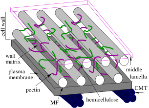
Figure 2. Schematic diagram of a plant cell wall. MF denotes cell wall microfibrils, CMT denotes cortical microtubules in a plant cell.

In our model we focus on two aspects which have not been considered together before: the influence of the microstructure, associated with the cellulose microfibrils, and of the calcium-pectin cross-links on the mechanical properties of plant cell walls. In the microscopic model of cell wall biomechanics derived here, the cell wall microstructure and the dynamics of the formation and dissociation of calcium-pectin cross-links are considered explicitly.

It is supposed that calcium-pectin cross-linking chemistry is one of the main regulators of cell wall elasticity and extension [61]. It has been shown that the modification of pectin by PME and the control of the amount of calcium-pectin cross-links greatly influence the mechanical deformations of plant cell walls [46, 47], and the interference with PME activity causes dramatic changes in growth behavior of plant cells and tissues [62]. We consider the most abundant subclass of pectin, homogalacturonan, which is important for the regulation of plant biomechanics and growth. Homogalacturonan consists of a long linear chain of galacturonic acids. Pectin is deposited into the cell wall in a highly methylestrified state and then is modified by the enzyme pectin-methylesterase (PME), which removes methyl groups [60]. The demethylesterified pectin interacts with calcium ions to produce load bearing cross-links, which reduce cell wall expansion, see e.g. [61].

In the mathematical model a flat section of a cell wall composed of a polysaccharide matrix and cellulose microfibrils is considered. Let $\Omega$ be a reference configuration of the plant cell wall. The domains $\Omega_{M}$ and $\Omega_{F}$ denote the parts of $\Omega$ occupied by the cell wall matrix and microfibrils, respectively.

We consider five species within the plant cell wall matrix: methylestrified pectin, the enzyme PME, demethyl-estrified pectin, calcium ions, and calcium-pectin cross-links. To form cross-links with calcium ions Ca²⁺, pectin molecules need to have only some of their constituent acids de-estrified, see e.g. [15, 60]. Thus, when describing the density of pectin in the different states, we refer to the density of the galacturonic acid groups in the different states.

Let $n_{e}$, $n_{E}$, $n_{d}$, $n_{c}$, and $n_{b}$ denote the number densities of methylestrified pectin acid groups, PME enzyme, demethylestrified pectin acid groups, calcium ions, and calcium-pectin cross-links in the reference configuration $\Omega_{M}$, respectively. Let $S=\{e,E,d,c,b\}$ be an index set and $n_{S}$ will denote all five of the densities. We assume that the densities $n_{\alpha}$, with $\alpha\in S$, are changing due to spacial movement, reactions between the species, and external agencies. Thus, the balance equation for $n_{\alpha}$ is given by

(77) $$\partial_{t}n_{\alpha}=r_{\alpha}-\text{div}\,{\bf j}_{\alpha}+h_{\alpha}\qquad\text{in}\;\;\Omega_{M},\qquad\qquad\alpha\in S,$$

where $r_{\alpha}$ models the chemical reactions between the species, ${\bf j}_{\alpha}$ is the flux, and $h_{\alpha}$ is the species supply due to external agencies. The momentum balance for the cell wall reads

(78) $$\textbf{0}=\text{div}\,{\bf T}_{\text{R}}+{\bf b}\qquad\text{in}\ \Omega,$$

where ${\bf T}_{R}$ is the Piola stress and ${\bf b}$ denotes the external body forces, including inertial forces. We consider elastic behavior of the wall material and assume that the chemical processes in the wall matrix influence the mechanical properties of the cell walls, see e.g. [15, 60]. The constitutive law of linear elasticity, see e.g. [10], for the stress is assumed:

(79) $${\bf T}_{\text{R}}=\big{(}\mathbb{E}_{M}(n_{S})\chi_{\Omega_{M}}+\mathbb{E}_{F}\chi_{\Omega_{F}}\big{)}{\bf e}({\bf u}),$$

where $\mathbb{E}_{M}(n_{S})$ and $\mathbb{E}_{F}$ are elasticity tensors for cell wall matrix and microfibrils, respectively, and ${\bf e}({\bf u})=\frac{1}{2}(\nabla{\bf u}+\nabla{\bf u}^{\rm T})$ is the symmetric part of the displacement gradient, $\chi_{A}$ is the characteristic function of a domain $A$.

The interactions between the mechanical properties of the cell wall and the biochemistry of the wall matrix are also reflected in the reactions terms

(80) $$r_{\alpha}=r_{\alpha 0}(n_{S})+{\bf Z}_{\alpha}(n_{S})\cdot\widetilde{\mathcal{N}}_{\delta}({\bf e}({\bf u})),$$

where

$$\widetilde{\mathcal{N}}_{\delta}({\bf e}({\bf u}))(x)=\mathchoice{{\vbox{\hbox{$\textstyle-$ }}\kern-7.57222pt}}{{\vbox{\hbox{$\scriptstyle-$ }}\kern-5.70335pt}}{{\vbox{\hbox{$\scriptscriptstyle-$ }}\kern-4.59167pt}}{{\vbox{\hbox{$\scriptscriptstyle-$ }}\kern-4.10834pt}}\!\int_{B_{\delta}(x)\cap\Omega}\mathbb{E}(n_{S}){\bf e}({\bf u})(\tilde{x})d\tilde{x}$$

for all $x\in\overline{\Omega}$, with $\mathbb{E}(n_{S})=\mathbb{E}_{M}(n_{S})\chi_{\Omega_{M}}+\mathbb{E}_{F}\chi_{\Omega_{F}}$. We assume that the stress influences the chemical reactions and the dynamics of calcium-pectin cross-links [48]. Since pectin are long molecules, we assume the nonlocal impact of cell wall mechanics on chemical processes. Thus, stresses within a neighborhood of a point affect the rate of the chemical reactions. The length scale $\delta$ is associated with the length of the pectin molecules.

The flux of species $\alpha$ is assumed to be determined by Fick’s law:

(81) $${\bf j}_{\alpha}=-{\bf D}_{\alpha}\nabla n_{\alpha},$$

where ${\bf D}_{\alpha}$ is the diffusion coefficient of the species $\alpha$.

Next, we specify assumptions on the constitutive laws introduced in (79)–(81) that reflect the physics of the plant cell wall. The cell wall matrix has the same properties in all directions and, hence, is isotropic, see e.g. [64]. This is expressed mathematically by requiring

(82) $$\left.\begin{aligned} \mathbb{E}_{M}(n_{S})({\bf Q}{\bf e}({\bf u}){\bf Q}^{\rm T})&={\bf Q}(\mathbb{E}_{M}(n_{S}){\bf e}({\bf u})){\bf Q}^{\rm T},\\ {\bf Z}_{\alpha}(n_{S})&={\bf Q}{\bf Z}_{\alpha}(n_{S}){\bf Q}^{\rm T},\\ {\bf D}_{\alpha}&={\bf Q}{\bf D}_{\alpha}{\bf Q}^{\rm T},\end{aligned}\right\}\ \text{for all rotations}\ {\bf Q}.$$

Using standard representation theorems for isotropic functions, see e.g. [24], equations (82) imply that

(83) $$\mathbb{E}_{M}(n_{S}){\bf e}({\bf u}) =2\mu(n_{S}){\bf e}({\bf u})+\lambda(n_{S})(\text{div}\,{\bf u})\textbf{1},$$

$${\bf Z}_{\alpha}(n_{S}) =z_{\alpha}(n_{S})\textbf{1},$$

$${\bf D}_{\alpha} =D_{\alpha}\textbf{1}.$$

While it is known that polymers can diffuse [25], the diffusion coefficient of calcium-pectin cross-links is much lower than the diffusion coefficients of the other species and, thus, we assume first that calcium-pectin cross-links do not diffuse, i.e. $D_{b}=0$. Unlike the matrix, the microfibrils have different elastic properties in different directions, see e.g. [16]. For a plant cell wall, the amount of calcium-pectin cross-links plays a decisive role in determining the elastic properties of the wall matrix, [56, 61]. Thus, we assume that $\mathbb{E}_{M}$ or, equivalently, $\mu$ and $\lambda$, depends only on $n_{b}$.

We consider the following four interactions between the species in the matrix:

1. The enzyme PME interacts with methylestrified pectin to form demethylestrified pectin.

2. Demethylestrified pectin decays.

3. Demethylestrified pectin and calcium ions bind together to form calcium-pectin cross-links.

4. Under the presence of stress, calcium-pectin cross-links break to yield demethylestrified pectin and calcium ions.

For a detailed discussion of Interactions 1–4, see e.g. [48, 60, 64].

We begin by discussing the reaction term $r_{d}$, which is decomposed into the sum of three terms:

$$r_{d}=r_{eE}+r_{dd}+r_{fb},$$

where $r_{eE}$ is the rate of change of the density of demethylestrified pectin acid groups, $n_{d}$, associated with Interaction 1, $r_{dd}$ is the rate of decay of $n_{d}$ mentioned in Interaction 2, and $r_{fb}$ is the rate of change of $n_{d}$ associated with the formation and breakage of calcium-pectin cross-links specified in Interactions 3 and 4.

From Interaction 1, we have

$$r_{eE}=-r_{e}.$$

We assume that the binding of PME to and dissociation from a pectin acid group are very fast, and that the enzyme PME is not used up during the demethyl-esterification process so that $r_{E}=0$. From Interactions 3 and 4 it follows that

$$r_{b}=-r_{c}=-\frac{1}{2}r_{fb}.$$

The factor of a half in front of $r_{fb}$ reflects the fact that two demethylestirified galacturonic acids are needed to form a calcium-pectin cross-link. We assume that

$$r_{eE} =R_{eE}(n_{e},n_{E}),$$

$$r_{dd} =-R_{d}\,n_{d},$$

where $R_{eE}$ defines the demethyl-esterification reaction between methylestrified galacturonic acid groups and PME and $R_{d}>0$ is a decay constant of the demethylestrified pectin. Interactions between demethylestirified pectin and calcium ions increase the number of cross-links, while stress can break the cross-links. Thus

(84) $$r_{b} =R_{dc}(n_{d},n_{c})-R_{b}(n_{b})\,{{\mathcal{N}}}_{\delta}({\bf e}({\bf u})),$$

where $R_{dc}$ models the formation of cross-links through the interactions between demethylesterified pectin and calcium ions, and ${{\mathcal{N}}}_{\delta}({\bf e}({\bf u}))$ is defined as

(85) $$\mathcal{N}_{\delta}({\bf e}({\bf u}))(t,x)=\Big{(}\mathchoice{{\vbox{\hbox{$\textstyle-$ }}\kern-7.57222pt}}{{\vbox{\hbox{$\scriptstyle-$ }}\kern-5.70335pt}}{{\vbox{\hbox{$\scriptscriptstyle-$ }}\kern-4.59167pt}}{{\vbox{\hbox{$\scriptscriptstyle-$ }}\kern-4.10834pt}}\!\int_{B_{\delta}(x)\cap\Omega}\text{tr }\mathbb{E}(n_{b})\,{\bf e}({\bf u})(t,\tilde{x})\,d\tilde{x}\Big{)}^{+}\qquad\text{for all }\;x\in\overline{\Omega}\text{ and }t\in(0,T).$$

Having $r_{b}$ depend on the positive part of the local average of the stress does not follow from (80), but it is consistent with the isotropy assumption. The reason for the choice (84) is based on the idea that stretching, rather than compressing, of the cross-links will cause them to break.

Possible choices for the functions $R_{eE}$, $R_{dc}$, and $R_{b}$ are

$$R_{eE}(n_{e},n_{E})=k_{eE}n_{e}n_{E}, \quad R_{dc}(n_{d},n_{c})=\frac{k_{dc,1}n_{c}}{k_{dc,2}+n_{c}}n_{d}, \quad R_{b}(n_{b})=k_{b}n_{b},$$

where $k_{eE}$, $k_{dc,1}$, $k_{dc,2}$, and $k_{b}$ are positive constants. Due to the high calcium concentration in plant cell walls, we assume saturation kinetics for the density of calcium ions in the reaction term $R_{dc}$.

Remark. The constitutive laws, considered here, are consistent with the Second Law of Thermodynamics in that, in the elastic case, Maxwell’s relation

$$\frac{\partial{\bf T}_{R}}{\partial n_{\alpha}}=\frac{\partial\mu_{\alpha}}{\partial{\bf e}({\bf u})}$$

holds, where $\mu_{\alpha}$ is the chemical potential for species $\alpha$, which depends on $n_{S}$, and ${\bf e}({\bf u})$, see [24]. The chemical potential is related to the flux ${\bf j}_{\alpha}$ through the relation

$${\bf j}_{\alpha}=-{\bf M}_{\alpha}\nabla\mu_{\alpha}.$$

To obtain the flux used in this section, set

$$\mu_{\alpha} =\begin{cases}n_{\alpha}&\qquad\alpha\not=b,\\ \dfrac{1}{2}{\bf e}({\bf u})\cdot\dfrac{\partial\mathbb{E}}{\partial n_{b}}(n_{b}){\bf e}({\bf u})&\qquad\alpha=b,\end{cases}$$

$${\bf M}_{\alpha} =\begin{cases}D_{\alpha}\textbf{1}&\qquad\alpha\not=b,\\ 0&\qquad\alpha=b.\end{cases}$$

The environment can effect the cell wall in two different ways: through external influences and boundary conditions. The effects of the supply of species $h_{\alpha}$ and external body forces ${\bf b}$, including inertial terms, are neglected so

$$h_{\alpha}=0\ \ \text{in}\ \Omega_{M}\qquad\text{and}\qquad{\bf b}=\textbf{0}\ \ \text{in}\ \Omega.$$

The boundary $\partial\Omega$ of $\Omega$ is decomposed into four disjoint surfaces: $\Gamma_{\mathcal{I}}$, $\Gamma_{\mathcal{E}}$, $\Gamma_{{\mathcal{U}}}$, and $\partial\Omega\setminus(\Gamma_{\mathcal{I}}\cup\Gamma_{\mathcal{E}}\cup\Gamma_{\mathcal{U}})$, where $\Gamma_{\mathcal{I}}$ is the part of $\partial\Omega$ in contact with the interior of the cell and $\Gamma_{\mathcal{E}}$ is the part of $\partial\Omega$ in contact with the middle lamella. Let $\boldsymbol{\nu}$ denote the exterior unit-normal to whatever surface is under discussion. On $\Gamma=\partial\Omega_{F}\setminus\partial\Omega$, $\boldsymbol{\nu}$ points away from $\Omega_{M}$.

PME, produced in the Golgi apparatus of a plant cell, is deposited into the cell wall and diffuses through the cell wall into the middle lamella. PME can also diffuse back into the cell to degrade. Thus, we assume that the enzyme PME can enter or leave the cell wall through $\Gamma_{\mathcal{I}}$ but can only leave the wall through $\Gamma_{\mathcal{E}}$. To account for the mechanisms controlling the amount of PME in a cell wall [61], we assume that the inflow of PME into the cell wall depends on the total amount of methylestrified pectin within the wall, which leads to the boundary fluxes

$${\bf j}_{E}\cdot\boldsymbol{\nu} =-J_{E}\Big{(}\int_{\Omega_{M}}n_{e}\,dx\Big{)}+\zeta_{E}n_{E} \qquad\text{on}\ \Gamma_{\mathcal{I}},$$

$${\bf j}_{E}\cdot\boldsymbol{\nu} =\gamma_{E}n_{E} \qquad\text{on}\ \Gamma_{\mathcal{E}},$$

where $\zeta_{E}$ and $\gamma_{E}$ are non-negative constants.

Methylesterified pectin is produced by the cell and then transported into the cell wall through $\Gamma_{\mathcal{I}}$, e.g. [60]. To account for mechanisms controlling the amount of pectin in the cell wall, we assume that the inflow of new methylestrified pectin decreases with an increasing amount of methylestrified pectin in the wall. Methylestrified pectin can leave the wall through $\Gamma_{\mathcal{E}}$ and enter the middle lamella. Thus,

(86) $${\bf j}_{e}\cdot\boldsymbol{\nu} =-J_{e}\Big{(}\int_{\Omega_{M}}n_{e}\,dx\Big{)} \qquad\text{on}\ \Gamma_{\mathcal{I}},$$

$${\bf j}_{e}\cdot\boldsymbol{\nu} =\gamma_{e}n_{e} \qquad\text{on}\ \Gamma_{\mathcal{E}},$$

where $\gamma_{e}$ is a non-negative constant. We assume an outflow of demethylesterified pectin from the cell wall into the middle lamella:

(87) $${\bf j}_{d}\cdot\boldsymbol{\nu}=0\qquad\text{on}\ \Gamma_{\mathcal{I}},\qquad\qquad{\bf j}_{d}\cdot\boldsymbol{\nu}=\gamma_{d}n_{d}\qquad\text{on}\ \Gamma_{\mathcal{E}}.$$

Calcium ions may enter or leave the cell wall through both $\Gamma_{\mathcal{I}}$ and $\Gamma_{\mathcal{E}}$, but the flow of calcium through $\Gamma_{\mathcal{I}}$ is controlled by stretch activated calcium channels in the plasma membrane, see e.g. [18, 59]. Thus, the flow of calcium through $\Gamma_{\mathcal{I}}$ is assumed to depend on the local average of the stress and on the density of calcium, so that

(88) $${\bf j}_{c}\cdot\boldsymbol{\nu} =-J_{c,{\mathcal{E}}}(n_{c}) \text{on }\Gamma_{\mathcal{E}},$$

$${\bf j}_{c}\cdot\boldsymbol{\nu} =-{{\mathcal{N}}}_{\delta}({\bf e}({\bf u}))\,J_{c,{\mathcal{I}}}(n_{c}) \text{on}\ \Gamma_{\mathcal{I}},$$

where

$$J_{c,{\mathcal{I}}}(n_{c})=\gamma_{c,1}-\gamma_{c,2}n_{c},\qquad\qquad J_{c,{\mathcal{E}}}(n_{c})=\zeta_{c,1}-\zeta_{c,2}n_{c},$$

with non-negative constants $\gamma_{c,i}$ and $\zeta_{c,i}$, where $i=1,2$, and ${\mathcal{N}}_{\delta}({\bf e}({\bf u}))$ is given by (85). Similar to (84), we assume that the right-hand side of (88)₂ depends on the positive part of the local average of the stress.

The traction boundary conditions

$${\bf T}_{R}\boldsymbol{\nu} =-p_{\mathcal{I}}\boldsymbol{\nu} \qquad\text{on}\ \Gamma_{\mathcal{I}},\qquad\qquad {\bf T}_{R}\boldsymbol{\nu}={\bf f} \qquad\text{on}\ \Gamma_{\mathcal{E}}\cup\Gamma_{\mathcal{U}},$$

come from the constant, positive turgor pressure $p_{\mathcal{I}}$ within the cell and the traction force ${\bf f}$, caused by surrounding cells. We consider zero-flux boundary conditions on the surface of the microfibrils and on $\Gamma_{\mathcal{U}}$:

$${\bf j}_{\alpha}\cdot\boldsymbol{\nu}=0\qquad\text{on}\ \Gamma\qquad\quad\text{ and }\quad\qquad{\bf j}_{\alpha}\cdot\boldsymbol{\nu}=0\qquad\text{on}\ \Gamma_{\mathcal{U}},\qquad\alpha=e,E,d,c.$$

On $\partial\Omega\setminus(\Gamma_{\mathcal{I}}\cup\Gamma_{\mathcal{E}}\cup\Gamma_{\mathcal{U}})$ periodic boundary conditions for the densities and displacement are imposed.

Possible choices for the functions that determine the boundary conditions are

$$J_{E}\Big{(}\int_{\Omega_{M}}n_{e}\,dx\Big{)}=\beta_{E}\int_{\Omega_{M}}n_{e}\,dx,\qquad J_{e}\Big{(}\int_{\Omega_{M}}n_{e}\,dx\Big{)}=\frac{\beta_{e}}{1+\zeta_{e}\int_{\Omega_{M}}n_{e}\ dx},$$

$${\bf f}=p_{{\mathcal{E}}}\,\boldsymbol{\nu}\quad\text{ on }\Gamma_{\mathcal{E}},\qquad{\bf f}=p_{{\mathcal{U}}}\,\boldsymbol{\nu}\quad\text{ on }\Gamma_{\mathcal{U}},$$

where $\beta_{E}$, $\beta_{e}$, $\zeta_{e}$, $p_{\mathcal{E}}$, and $p_{\mathcal{U}}$ are positive constants.

The difference between Model I and Model II is that in Model II we assume that the calcium-pectin cross-links can diffuse, i.e. $D_{b}>0$. In this situation we assume that the reaction term associated with the formation and destruction of cross-links depends on the point-wise values of the displacement gradient rather than the local average:

(89) $$r_{b} =R_{dc}(n_{d},n_{c})-R_{b}(n_{b})\,Q(n_{b},{\bf e}({\bf u})),$$

where a possible choice for $Q$ is $Q(n_{b},{\bf e}({\bf u}))=\big{(}{\rm tr}\,\mathbb{E}(n_{b})\,{\bf e}({\bf u})\big{)}^{+}$. Considering the diffusion of calcium-pectin cross-links corresponds to the situation where the calcium-pectin network is less connected and the mechanical stress in the cell wall have a point-wise impact on chemical processes.

10. Summary

In this paper we developed a mathematical model for plant cell wall biomechanics which explicitly considers the microscopic structure of the cell wall and the biochemical processes that take place within the wall matrix. The microscopic model defined on the scale of the cell wall’s structural elements describes the interconnections between the calcium-pectin cross-links dynamics and the changes in the mechanical properties of the cell wall. We consider both a non-local effect of strain or stress on the calcium-pectin cross-link dynamics as well as a point-wise dependence of chemical reactions on mechanical forces. Applying homogenization techniques we rigorously derive macroscopic models for plant cell wall biomechanics. We also show that since the cell wall matrix is isotropic, the macroscopic elasticity tensor is a linear function of the Young’s modulus of the wall matrix. Then assuming that only the Young’s modulus of the wall matrix depends on the density of calcium-pectin cross-links we compute numerically the effective macroscopic elastic properties of the plant cell wall as a function of the density of calcium-pectin cross-links. In the numerical simulations, the cell wall microfibrils are assumed to be transversal isotropic. The numerical analysis of the full macroscopic model will be the subject of future research.

Acknowledgements. The authors would like to thank Dr. Sebastian Wolf for fruitful discussions on the molecular biology of plant cell walls.

References

• [1] E. Acerbi, V. Chiado Piat, G. Dal Maso and D. Percivale, An extension theorem from connected sets, and homogenization in general periodic domains, Nonlin. Anal. Theory, Methods, Applic. 18 (1992) 481–496.
• [2] Alikakos N.D. $L^{p}$ bounds of solutions of reaction-diffusion equations, Comm. Partical Differential Equations. 4 (1976) 827–868.
• [3] G. Allaire, Homogenization and two-scale convergence, SIAM J. Math. Anal. 23 (1992) 1482–1518.
• [4] G. Allaire, Shape Optimization by the Homogenization Method, (Springer, 2002).
• [5] A. Bensoussan, J.-L. Lions and G. Papanicolaou, Asymptotic Analysis for Periodic Structures, (North Holland, 1978).
• [6] H. Brezis, Functional Analysis, Sobolev Spaces and Partial Differential Equations, (Springer, 2010).
• [7] Chavarría-Krauser A., Ptashnyk M. Homogenization approach to water transport in plant tissues with periodic microstructures. Math. Model. Nat. Phenom. 8 (2013) 80–111.
• [8] M.-A.-J. Chaplain, The strain energy function of an ideal plant cell wall, Journal of Theoretical Biology 163 (1993) 77–97.
• [9] P.-G. Ciarlet and P. Ciarlet Jr., Another approach to linear elasticity and Korn’s inequality, C.R. Acad. Sci. Paris Ser. I 339 (2004) 307–312.
• [10] P.-G. Ciarlet, Mathematical elasticity. Volume I: Three-dimensional elasticity, (North-Holland, 1988).
• [11] D. Cioranescu, A. Damlamian and G. Griso, The periodic unfolding method in homogenization, SIAM Journal of Mathematics and Analysis 40 (2008) 1585–1620.
• [12] D. Cioranescu, A. Damlamian, P. Donato, G. Griso, and R. Zaki, The periodic unfolding method in domains with holes, SIAM J. Math. Anal. 44 (2012) 718–760.
• [13] D. Cioranescu and J. Saint Jean Paulin, Homogenization of reticulated structures, (Springer, 1999).
• [14] J.-R. Colvin, The size of the cellulose microfibril, Journal of Cell Biology (1963) 17 105–109.
• [15] D.-J. Cosgrove, Growth of the plant cell wall, Nature Reviews Molecular Cell Biology 6 (2005) 850–86.
• [16] I. Diddens, B. Murphy, M Krisch and M. Müller, Anisotropic elastic properties of cellulose measured using inelastic X-ray scattering, Macromolecules 41 (2008) 9755–9759.
• [17] J. Dumais, S.-L. Shaw, C.-R. Steele, S.-R. Long and P.-M. Ray, An anisotropic-viscoplastic model of plant cell morphogenesis by tip growth, The International Journal of Developmental Biology 50 (2006) 209–222.
• [18] R. Dutta and K.-R. Robinson, Identification and characterization of stretch-activated ion channels in pollen protoplasts, Plant Physiology 135 (2004) 1398–1406.
• [19] R.-J. Dyson, L.-R. Band and O.-E. Jensen, A model of crosslink kinetics in the expanding plant cell wall: Yield stress and enzyme action, J. of Theor. Biol. 307 (2012) 125–136.
• [20] R.-J. Dyson, O.-E. Jensen, A fibre-reinforced fluid model of anisotropic plant cell growth, J. of Fluid Mech. 655 (2010) 472–503.
• [21] T. Fatima, A. Muntean and M. Ptashnyk, Error estimate and unfolding method for homogenization of a reaction-diffusion system modeling sulfate corrosion, Applicable Analysis 91 (2012) 1129–1154.
• [22] Y.C. Fung, Biomechanics: mechanical properties of living tissues, (Springer, 1993).
• [23] R.-P. Gilbert and A. Mikelić, Homogenizing the acoustic properties of the seabed: Part I, Nonlinear Analysis 40 (2000) 185–212.
• [24] M.-E. Gurtin, E. Fried and L. Anand, The Mechanics and Thermodynamics of Continua, (Cambridge University Press, 2010).
• [25] L. Haggerty, J.H. Sugarman, R.K. Prud’homme, Diffusion of polymers through polyacrylamide gels, Polymer, 29 (1988) 1058–1063.
• [26] W. Jäger and U. Hornung, Diffusion, convection, adsorption, and reaction of chemicals in porous media, J. Differ. Equations 92 (1991) 199–225.
• [27] W. Jäger, A. Mikelić and M. Neuss-Radu, Homogenization limit of a model system for interaction of flow, chemical reactions, and mechanics in cell tissues, SIAM J. Math. Anal. 43 (2011) 1390–1435.
• [28] V.-V. Jikov, S.-M. Kozlov and O.-A. Oleinik, Homogenization of Differential Operators and Integral Functionals, (Springer, 1994).
• [29] C.-J. Jennedy, A. S̆turcová, M.-C. Jarvis and T.-J. Wess, Hydration effects on spacing of primary-wall cellulose microfibrils: a small angle X-ray scattering study, Cellulose 14 (2007) 401–408.
• [30] A. Korn, Über einige ungleichungen, welche in der theorie del elastichen und elektrishen schwingungen eine rolle spielen, Bullettin Internationale, Cracovie Akademie Umiejet, Classe des sciences mathématiques et naturelles (1909) 705–724.
• [31] J.-H. Kroeger, R. Zerzour and A. Geitmann, Regulator or driving force? The role of turgor pressure in oscillatory plant cell growth, PLoS ONE 6 (2011) e18549.
• [32] Ladyzhenskaya O., Solonnikov V., Ural’ceva N. Linear and quasilinear equations of parabolic type. American Mathematical Society, 1968.
• [33] J.-L. Lions, Quelques Méthodes de Résolution des Problèmes aux Limites Non Linéaires, (Dunod, 1969).
• [34] A. Logg, K.-A. Mardal, G.N. Wells et al. Automated solution of differential equations by the finite element method, (Springer, 2012).
• [35] A. Logg and G.N. Wells, DOLFIN: automated finite element computing, ACM Transactions on Mathematical Software, 37 (2010).
• [36] A.J. Majda, A.L. Bertozzi Vorticity and Incompressible Flow, Cambridge Texts in Applied Mathematics, 2001.
• [37] A. Marciniak-Czochra and M. Ptashnyk, Derivation of a macroscopic receptor-based model using homogenisation techniques, SIAM J. Math. Anal. 40 (2008) 215–237.
• [38] M.-L. Mascarenhas, Homogenization of a viscoelastic equations with non-periodic coefficients, Proceedings of the Royal Society of Edinburgh: Section A Mathematics 106 (1987) 143–160.
• [39] A. Mikelić and M.-F. Wheeler, On the interface law between a deformable porous medium containing a viscous fluid and an elastic body, Math. Models Methods Appl. Sci. 22 (2012) 1250031.
• [40] F. Murat and L. Tartar, H-convergence, in Topics in the Mathematical Modelling of Composite Materials, Progr. Nonlinear Differential Equations Appl. 31, Birkhäuser Boston, Boston, MA, 1997, pp. 21 43.
• [41] J. Necas, Les méthodes directes en théorie des équations elliptiques, (Academie, Prague, 1967).
• [42] G. Nguetseng, A general convergence result for a functional related to the theory of homogenization, SIAM J. Math. Anal. 20 (1989) 608–623.
• [43] O. Oleinik, A.-S. Shamaev and G.-A. Yosifian, Mathematical problems in Elasticity and Homogenization, (North Holland, 1992).
• [44] K.B. Ølgaard and G. N. Wells, Optimisations for quadrature representations of finite element tensors through automated code generation, ACM Transactions on Mathematical Software, 37 (2010).
• [45] J.-B. Passioura and S.-C. Fry, Turgor and cell expansion: beyond the Lockhart equation, Aust. J. Plant Physiol. 19 (1992) 565–576.
• [46] A. Peaucelle, S.A. Braybrook, L. Le Guillou, E. Bron, C. Kuhlemeier and H. Hofte, Pectin-induced changes in cell wall mechanics underlie organ initiation in Arabidopsis, Curr. Biol. 21 (2011) 1720–1726.
• [47] S. Pelletier, J. Van Orden, S. Wolf, K. Vissenberg, J. Delacourt, Y.-A. Ndong, J. Pelloux, V. Bischoff, A. Urbain, G. Mouille, G. Lemonnier, J.-P. Renou and H. Hofte, A role for pectin de-methylesterification in a developmentally regulated growth acceleration in dark-grown Arabidopsis hypocotyls, New Phytol 188 (2010) 726–739.
• [48] T.-E. Proseus and J.-S. Boyer, Calcium deprivation disrupts enlargement of Chara corallina cells: further evidence for the calcium pectate cycle, J. of Exp. Bot. 63 (2012) 1–6.
• [49] M. Ptashnyk, Derivation of a macroscopic model for nutrient uptake by a single branch of hairy-roots. Nonlinear Analysis: Real World Applic. 11 (2010) 4586–4596.
• [50] M. Ptashnyk and B. Seguin, Periodic homogenization and material symmetry in linear elasticity, arXiv:1504.08165 , 2015.
• [51] R. Redlinger, Invariant sets for strongly coupled reaction-diffusion systems under general boundary conditions, Arch. Rational Mech. Anal. 108 (1989) 281–291.
• [52] E.-R. Rojas, S. Hotton and J. Dumais, Chemically mediated mechanical expansion of the pollen tube cell wall, Biophys. J. 101 (2011) 1844–1853.
• [53] E. Sanchez-Palencia, Non-Homogeneous Media and Vibration Theory, (Springer, 1980).
• [54] J. Simon, Compact sets in the space $L^{p}(0,T;B)$, Annali di Matematica pure ed applicata, (IV), Vol. CXLVI (1987) 65–96.
• [55] J. Smoller, Shocke Waves and Reaction-Diffusion Equations, (Springer 1994).
• [56] C. Somerville, S. Bauer, G. Brininstool, M. Facette, T. Hamann, J. Milne, E. Osborne, A. Paredez, S. Persson, T. Raab, S. Vorwerk and H. Youngs, Toward a systems approach to understanding plant cell walls, Science 306 (2004) 2206.
• [57] L.-H. Thomas, V.-T. Forsyth, A. S̆turcová, C.-J. Kennedy, R.-P. May, C.-M. Altaner, D.-C. Apperley, T.-J. Wess and M.-C. Jarvis, Structure of cellulose microfibrils in primary cell walls from collenchyma, Plant Physiology 161 (2013) 465–476.
• [58] B.-A. Veytsman and D.-J. Cosgrove, A model of cell wall expansion based on thermodynamics of polymer networks, Biophys. J. 75 (1998) 2240–2250.
• [59] P.J. White, The pathways of calcium movement to the xylem, J. Exp. Bot. 52 (2001) 891–899.
• [60] S. Wolf and S. Greiner, Growth control by cell wall pectins, Protoplasma 249 (2012) 169–175.
• [61] S. Wolf, K. Hématy and H. Höfte, Growth control and cell wall signaling in plants, Annu. Rev. Plant Biol. 63 (2012) 381–407.
• [62] S. Wolf, J. Mravec, S. Greiner, G. Mouille and H. Höfte, Plant cell wall homeostasis is mediated by Brassinosteroid feedback signaling, Curr. Biol. 22 (2012) 1732–1737.
• [63] U.-Z. Zimmermann, D. Hüs ken and E.-D. Schulze, Direction turgor pressure measurements in individual leave cells of Tradescantia virginiana, Planta 148 (1980) 445–453.
• [64] G. Zsivanovits, A.-J. MacDougall, A.-C. Smith, S.-G. Ring, Material properties of concentrated pectin networks, Carbohyd. Res. 339 (2004) 1317–1322.