Fourth-moment Analysis for Wave Propagation in the White-Noise Paraxial Regime

Abstract

In this paper we consider the Itô-Schrödinger model for wave propagation in random media in the paraxial regime. We solve the equation for the fourth-order moment of the field in the regime where the correlation length of the medium is smaller than the initial beam width. As applications we prove that the centered fourth-order moments of the field satisfy the Gaussian summation rule, we derive the covariance function of the intensity of the transmitted beam, and the variance of the smoothed Wigner transform of the transmitted field. The second application is used to explicitly quantify the scintillation of the transmitted beam and the third application to quantify the statistical stability of the Wigner transform.

AMS subject classifications. 60H15, 35R60, 74J20.

Key words. Waves in random media, parabolic approximation, scintillation, Wigner transform.

1 Introduction

In many wave propagation scenarios the medium is not constant, but varies in a complicated fashion on a scale that may be small compared to the total propagation distance. This is the case for wave propagation through the turbulent atmosphere, the earth’s crust, the ocean, and complex biological tissue for instance. If one aims to use transmitted or reflected waves for communication or imaging purposes it is important to characterize how such microstructure affects and corrupts the wave. Such a characterization is particularly important for modern imaging techniques such as seismic interferometry or coherent interferometric imaging that correlate wave field traces that have been strongly corrupted by the microstructure and use their space-time correlation function for imaging. The wave field correlations are second-order moments of the wave field and a characterization of the signal-to-noise ratio then involves a fourth-order moment calculation.

Motivated by the situation described above we consider wave propagation through time-independent media with a complex spatially varying index of refraction that can be modeled as the realization of a random process. Typically we cannot expect to know the index of refraction pointwise, but we may be able to characterize its statistics and we are interested in how the statistics of the medium affects the statistics of the wave field. In its most common form, the analysis of wave propagation in random media consists in studying the field $v$ solution of the scalar time-harmonic wave or Helmholtz equation

$$\Delta v+k_{0}^{2}n^{2}(z,{{\itbf x}})v=0,\quad\quad(z,{{\itbf x}})\in\mathbb{R}\times\mathbb{R}^{2},$$ (1.1)

where $k_{0}$ is the free space homogeneous wavenumber and $n$ is a randomly heterogeneous index of refraction. Since the index of refraction $n$ is a random process, the field $v$ is also a random process whose statistical behavior can be characterized by the calculations of its moments. Even though the scalar wave equation is simple and linear, the relation between the statistics of the index of refraction and the statistics of the field is highly nontrivial and nonlinear. In this paper we consider a primary scaling regime corresponding to long-range beam propagation and small-scale medium fluctuations giving negligible backscattering. This is the so-called white-noise paraxial regime, as described by the Itô-Schrödinger model, which is presented in Section 2. This model is a simplification of the model (1.1) since it corresponds to an evolution problem, but yet in the regime that we consider it describes the propagated field in a weak sense in that it gives the correct statistical structure of the wave field. The Itô-Schrödinger model can be derived rigorously from (1.1) by a separation of scales technique in the high-frequency regime (see [2] in the case of a randomly layered medium and [23, 24, 25] in the case of a three-dimensional random medium). It models many situations, for instance laser beam propagation [45], time reversal in random media [5, 38], underwater acoustics [46], or migration problems in geophysics [8]. The Itô-Schrödinger model allows for the use of Itô’s stochastic calculus, which in turn enables the closure of the hierarchy of moment equations [19, 29]. Unfortunately, even though the equation for the second-order moments can be solved, the equation for the fourth-order moments is very difficult and only approximations or numerical solutions are available (see [15, 28, 47, 50, 57] and [29, Sec. 20.18]).

Here, we consider a secondary scaling regime corresponding to the so-called scintillation regime and in this regime we derive explicit expressions for the fourth-order moments. The scintillation scenario is a well-known paradigm, related to the observation that the irradiance of a star fluctuates due to interaction of the light with the turbulent atmosphere. This common observation is far from being fully understood mathematically. However, experimental observations indicate that the statistical distribution of the irradiance is exponential, with the irradiance being the square magnitude of the complex wave field. Indeed it is a well-accepted conjecture in the physical literature that the statistics of the complex wave field becomes circularly symmetric complex Gaussian when the wave propagates through the turbulent atmosphere [51, 58], so that the irradiance is the sum of the squares of two independent real Gaussian random variables, which has chi-square distribution with two degrees of freedom, that is an exponential distribution. However, so far there is no mathematical proof of this conjecture, except in randomly layered media [18, Chapter 9]. The regime we consider here, which we refer to as the scintillation regime, gives results for the fourth-order moments that are consistent with the scintillation or Gaussian conjecture. We prove in Section 9 that the incoherent zero-mean wave field (i.e. the fluctuations of the wave field defined as the difference between the field and its expectation) has fourth-order moments that obey the Gaussian summation rule. As a result we can discuss the statistical character of the irradiance in detail in Section 10.

Certain functionals of the solution to the white-noise paraxial wave equation can be characterized in some specific regimes [3, 4, 12, 39]. An important aspect of such characterizations is the so-called statistical stability property which corresponds to functionals of the wave field becoming deterministic in the considered scaling regime. This is in particular the case in the limit of rapid decorrelation of the medium fluctuations (in both longitudinal and lateral coordinates). As shown in [3] the statistical stability also depends on the initial data and can be lost for very rough initial data even with a high lateral diversity as considered there. In [31, 32] the authors also consider a situation with rapidly fluctuating random medium fluctuations and a regime in which the so-called Wigner transform itself is statistically stable. The Wigner transform is known to be a convenient tool to analyze problems involving the Schrödinger equation [27, 43]. In Section 11 we are able to push through a detailed and quantitative analysis of the stability of this quantity using our results on the fourth-order moments. An important aspect of our analysis is that we are able to derive an explicit expression of the coefficient of variation of the smoothed Wigner transform as a function of the smoothing parameters, in the general situation in which the standard deviation can be of the same order as the mean. This is a realistic scenario, we are not deep into a statistical stabilization situation, but in a situation where the parameters of the problem give partly coherent but fluctuating wave functionals. Here we are for the first time able to explicitly quantify such fluctuations and how their magnitude can be controlled by smoothing of the Wigner transform. We believe that these results are important for the many applications where the smoothed Wigner transform appears naturally.

The outline of the paper is as follows: In Section 2 we introduce the Itô-Schrödinger model. In Section 3 we summarize our main results. In Sections 4-5 we describe the general equations for the moments of the field. In Section 6 we discuss the second-order moments. In Section 7 we introduce and analyze the fourth-order moments and the particular parameterization that will be useful to untangle these. In Section 8 we introduce the so-called scintillation regime where we can get an explicit characterization of the fourth-order moments via the main result of the paper presented in Proposition 8.1. Next we discuss three applications of the main result: In Section 9 we prove that the centered fourth-order moments satisfy the Gaussian summation rule, in Section 10 we compute the scintillation index, and in Section 11 we analyze the statistical stability of the smoothed Wigner transform.

2 The White-Noise Paraxial Model

Let us consider the time-harmonic wave equation with homogeneous wavenumber $k_{0}$, random index of refraction $n(z,{{\itbf x}})$, and source in the plane $z=0$:

$$\Delta v+k_{0}^{2}n^{2}(z,{{\itbf x}})v=-\delta(z)f({{\itbf x}})\,,$$ (2.1)

for ${{\itbf x}}\in\mathbb{R}^{2}$ and $z\in[0,\infty)$. Denote by $\lambda_{0}$ the carrier wavelength (equal to $2\pi/k_{0}$), by $L$ the typical propagation distance, and by $r_{0}$ the radius of the initial transverse source. The paraxial regime holds when the wavelength $\lambda_{0}$ is much smaller than the radius $r_{0}$, and when the propagation distance is smaller than or of the order of $r_{0}^{2}/\lambda_{0}$ (the so-called Rayleigh length). The white-noise paraxial regime that we address in this paper holds when, additionally, the medium has random fluctuations, the typical amplitude of the medium fluctuations is small, and the correlation length of the medium fluctuations is larger than the wavelength and smaller than the propagation distance. In this regime the solution of the time-harmonic wave equation (2.1) can be approximated by [24]

$$v(z,{{\itbf x}})=\frac{i}{2k_{0}}u(z,{{\itbf x}})\exp\big{(}ik_{0}z\big{)},$$

where $(u(z,{{\itbf x}}))_{z\in[0,\infty),{{\itbf x}}\in\mathbb{R}^{2}}$ is the solution of the Itô-Schrödinger equation

$$d{u}(z,{{\itbf x}})=\frac{i}{2k_{0}}\Delta_{{{\itbf x}}}{u}(z,{{\itbf x}})dz+\frac{ik_{0}}{2}{u}(z,{{\itbf x}})\circ d{B}(z,{{\itbf x}}),$$ (2.2)

with the initial condition in the plane $z=0$:

$${u}(z=0,{{\itbf x}})=f({{\itbf x}}).$$

Here the symbol $\circ$ stands for the Stratonovich stochastic integral and $B(z,{{\itbf x}})$ is a real-valued Brownian field over $[0,\infty)\times\mathbb{R}^{2}$ with covariance

$$\mathbb{E}[{B}(z,{{\itbf x}}){B}(z^{\prime},{{\itbf x}}^{\prime})]={\min\{z,z^{\prime}\}}{C}({{\itbf x}}-{{\itbf x}}^{\prime}).$$ (2.3)

The model (2.2) can be obtained from the scalar wave equation (2.1) by a separation of scales technique in which the three-dimensional fluctuations of the index of refraction $n(z,{{\itbf x}})$ are described by a zero-mean stationary random process $\nu(z,{{\itbf x}})$ with mixing properties: $n^{2}(z,{{\itbf x}})=1+\nu(z,{{\itbf x}})$. The covariance function $C({{\itbf x}})$ in (2.3) is then given in terms of the two-point statistics of the random process $\nu$ by

$${C}({{\itbf x}}):=\int_{-\infty}^{\infty}\mathbb{E}[\nu(z^{\prime}+z,{{\itbf x}}^{\prime}+{{\itbf x}})\nu(z^{\prime},{{\itbf x}}^{\prime})]dz.$$ (2.4)

The covariance function $C$ is assumed to satisfy the following hypothesis:

$$C\in L^{1}(\mathbb{R}^{2}) C(0)<\infty$$ and . (2.5)

The condition $C\in L^{1}(\mathbb{R}^{2})$ imposes that the Fourier transform $\hat{C}$ is continuous and bounded by Lebesgue dominated convergence theorem, and it is also nonnegative by Bochner’s theorem (it is the power spectral density of a stationary process). The condition $C(0)<\infty$ then shows that $\hat{C}\in L^{1}(\mathbb{R}^{2})$, and therefore $C$ is continuous and bounded.
The white-noise paraxial model is widely used in the physical literature. It simplifies the full wave equation (2.1) by replacing it with the initial value-problem (2.2). It was studied mathematically in [9], in which the solution of (2.2) is shown to be the solution of a martingale problem whose $L^{2}$-norm is preserved in the case $f\in L^{2}(\mathbb{R}^{2})$. The derivation of the Itô-Schrödinger equation (2.2) from the three-dimensional wave equation in randomly scattering medium is given in [24].

3 Main Result and Quasi Gaussianity

Modeling with the white-noise paraxial model is often motivated by propagation through randomly heterogeneous media. The typical objective for such modeling is to describe some communication or imaging scheme, say with an object buried in the random medium. In many wave propagation and imaging scenarii the quantity of interest is given by a quadratic quantity of the field $u$. For instance, in the time-reversal problems a wave field emitted by the source is recorded on an array, then time-reversed and re-propagated into the medium [17]. The forward and time-reversed propagation paths give rise to a quadratic quantity in the field itself for the re-propagated field. Moreover, in important imaging approaches, in particular passive imaging techniques [22], the image is formed based on computing cross correlations of the field measured over an array again giving a quadratic expression in the field for the quantity of interest, the correlations. In a number of situations, in particular in optics, the measured quantity is an intensity, again a quadratic quantity in the field. As we explain in Section 6 the expected value of such quadratic quantities can in the white-noise paraxial regime be computed explicitly. In imaging applications this allows to compute the mean image and assess issues like resolution. However, it is important to go beyond this description and calculate the signal-to-noise ratio which requires to compute a fourth-order moment of the wave field. Despite the importance of the signal-to-noise ratio hitherto no rigorous result has been available that accomplishes this task. Indeed explicit expressions for the fourth moments has been a long standing open problem. This is what we push through in this paper. In the context of design of imaging techniques this insight is important to make proper balance in between noise and resolution in the image. We remark that in certain regimes one may be able to prove statistical stability, that is, that the signal-to-noise ratio goes to infinity in the scaling limit [38, 39]. The results we present here are more general in the sense that we can actually describe a finite signal-to-noise ratio and how the parameters of the problem determine this.

To summarize and explicitly articulate the main result regarding the fourth-order moment we consider first the first and second order moments of $u$ in (2.2) in the context when $f(x)=\exp[-|{{\itbf x}}|^{2}/(2r_{0}^{2})]$. We use the notations for the first and second-order moments

$$\mu_{1}(z,{{\itbf x}}):=\mathbb{E}[u(z,{{\itbf x}})],\quad\mu_{2}(z,{{\itbf x}},{{\itbf y}}):=\mathbb{E}[u(z,{{\itbf x}})\overline{u(z,{{\itbf y}})}],$$ (3.1)

Note that $\mu_{2}$ is given explicitly in (6.9). For the second centered moment we use the notation:

$$\tilde{\mu}_{2}(z,{{\itbf x}},{{\itbf y}}):=\mu_{2}(z,{{\itbf x}},{{\itbf y}})-\mu_{1}(z,{{\itbf x}})\overline{\mu_{1}(z,{{\itbf y}})}.$$ (3.2)

Then, to obtain an expression for the fourth-order moment, one heuristic approach often used in the literature [13, 29] is to assume Gaussianity. Consider any complex circularly symmetric Gaussian process $(Z({{\itbf x}}))_{{\itbf x}}$ then we have [42] that the fourth-order moment can be expressed in terms of the second-order moments by the Gaussian summation rule as

$$\mathbb{E}\big{[}Z({{\itbf x}}_{1})Z({{\itbf x}}_{2})\overline{Z({{\itbf y}}_{1})Z({{\itbf y}}_{2})}\big{]} = \mathbb{E}\big{[}Z({{\itbf x}}_{1})\overline{Z({{\itbf y}}_{1})}\big{]}\mathbb{E}\big{[}Z({{\itbf x}}_{2})\overline{Z({{\itbf y}}_{2})}\big{]}$$ (3.3)

$$+\mathbb{E}\big{[}Z({{\itbf x}}_{1})\overline{Z({{\itbf y}}_{2})}\big{]}\mathbb{E}\big{[}Z({{\itbf x}}_{2})\overline{Z({{\itbf y}}_{1})}\big{]}.$$

If the centered field $u(z,{{\itbf x}})-\mu_{1}(z,{{\itbf x}})$ were a complex circularly symmetric Gaussian process, then the fourth-order moment of the field $u$ defined by:

$$\mu_{4}(z,{{\itbf x}}_{1},{{\itbf x}}_{2},{{\itbf y}}_{1},{{\itbf y}}_{2}):=\mathbb{E}[u(z,{{\itbf x}}_{1})u(z,{{\itbf x}}_{2})\overline{u(z,{{\itbf y}}_{1})u(z,{{\itbf y}}_{2})}]$$

would satisfy:

$$\mu_{4}(z,{{\itbf x}}_{1},{{\itbf x}}_{2},{{\itbf y}}_{1},{{\itbf y}}_{2})=\mu_{1}(z,{{\itbf x}}_{1})\mu_{1}(z,{{\itbf x}}_{2})\overline{\mu_{1}(z,{{\itbf y}}_{1})}\overline{\mu_{1}(z,{{\itbf y}}_{2})}$$

$$\quad+\mu_{1}(z,{{\itbf x}}_{1})\overline{\mu_{1}(z,{{\itbf y}}_{1})}\tilde{\mu}_{2}(z,{{\itbf x}}_{2},{{\itbf y}}_{2})+\mu_{1}(z,{{\itbf x}}_{2})\overline{\mu_{1}(z,{{\itbf y}}_{1})}\tilde{\mu}_{2}(z,{{\itbf x}}_{1},{{\itbf y}}_{2})$$

$$\quad+\mu_{1}(z,{{\itbf x}}_{1})\overline{\mu_{1}(z,{{\itbf y}}_{2})}\tilde{\mu}_{2}(z,{{\itbf x}}_{2},{{\itbf y}}_{1})+\mu_{1}(z,{{\itbf x}}_{2})\overline{\mu_{1}(z,{{\itbf y}}_{2})}\tilde{\mu}_{2}(z,{{\itbf x}}_{1},{{\itbf y}}_{1})$$

$$\quad+\tilde{\mu}_{2}(z,{{\itbf x}}_{1},{{\itbf y}}_{1})\tilde{\mu}_{2}(z,{{\itbf x}}_{2},{{\itbf y}}_{2})+\tilde{\mu}_{2}(z,{{\itbf x}}_{1},{{\itbf y}}_{2})\tilde{\mu}_{2}(z,{{\itbf x}}_{2},{{\itbf y}}_{1}),$$

or equivalently:

$$\mu_{4}(z,{{\itbf x}}_{1},{{\itbf x}}_{2},{{\itbf y}}_{1},{{\itbf y}}_{2}) = \mu_{2}(z,{{\itbf x}}_{1},{{\itbf y}}_{1})\mu_{2}(z,{{\itbf x}}_{2},{{\itbf y}}_{2})+\mu_{2}(z,{{\itbf x}}_{1},{{\itbf y}}_{2})\mu_{2}(z,{{\itbf x}}_{2},{{\itbf y}}_{1})$$ (3.4)

$$-\mu_{1}(z,{{\itbf x}}_{1})\mu_{1}(z,{{\itbf x}}_{2})\overline{\mu_{1}(z,{{\itbf y}}_{1})}\overline{\mu_{1}(z,{{\itbf y}}_{2})}.$$

This result is not correct in general. For instance, in the spot-dancing regime addressed in [9, 20, 21], the explicit calculation of the moments of all orders is carried out and exhibits non-Gaussian statistics, in particular, the intensity follows a Rice-Nakagami statistics. The spot-dancing regime is valid for a narrow initial beam, strong medium fluctuations, and short propagation distance:

$$r_{0}=r_{0}^{\prime}{\varepsilon},\quad C({{\itbf x}})={\varepsilon}^{-2}C^{\prime}({{\itbf x}}),\quad z=z^{\prime}{\varepsilon},$$

with ${\varepsilon}\ll 1$ and the primed quantities of order one.

We show however in this paper that in the so-called scintillation regime the Gaussian summation rule (3.4) is valid . The scintillation regime is discussed in detail in Section 8, it is characterized by a wide initial beam, a long propagation distance, and weak medium fluctuations:

$$r_{0}=r_{0}^{\prime}/{\varepsilon},\quad C({{\itbf x}})={\varepsilon}C^{\prime}({{\itbf x}}),\quad z=z^{\prime}/{\varepsilon},$$

with ${\varepsilon}\ll 1$ and the primed quantities of order one. Moreover, in the scintillation regime, if the source spatial profile is Gaussian with radius $r_{0}$:

$$f({{\itbf x}})=\exp\Big{(}-\frac{|{{\itbf x}}|^{2}}{2r_{0}^{2}}\Big{)},$$ (3.5)

then

$$\mu_{2}(z,{{\itbf x}},{{\itbf y}}) = \frac{r_{0}^{2}}{4\pi}\exp\left(-{\frac{k_{0}^{2}C({\bf 0})z}{4}}\right)\int_{\mathbb{R}^{2}}\exp\Big{(}-\frac{r_{0}^{2}|{\boldsymbol{\xi}}|^{2}}{4}+i\frac{{\boldsymbol{\xi}}\cdot({{\itbf x}}+{{\itbf y}})}{2}\Big{)}$$

$$\times\exp\Big{(}\frac{k_{0}^{2}}{4}\int_{0}^{z}{C}\big{(}{{\itbf x}}-{{\itbf y}}-{\boldsymbol{\xi}}\frac{z^{\prime}}{k_{0}}\big{)}dz^{\prime}\Big{)}d{\boldsymbol{\xi}}$$

and

$$\mu_{1}(z,{{\itbf x}})=\exp\left(-{\frac{|{{\itbf x}}|^{2}}{2r_{0}^{2}}}\right)\exp\left(-{\frac{k_{0}^{2}C({\bf 0})z}{8}}\right).$$

Note that, in the scintillation regime, the field is partially coherent: the coherent field (i.e., the mean field $\mu_{1}$) has an amplitude which is of the same order as the standard deviation of the zero-mean incoherent field (i.e., the fluctuations of the field $u-\mu_{1}$). The surprising result that we report in this paper is that the incoherent field behaves like a random field with Gaussian statistics, as far as the fourth-order moments are concerned.

Finally in the strongly scattering scintillation regime when $k_{0}^{2}{C}({\bf 0})z\gg 1$ so that the mean field $\mu_{1}$ is vanishing and the field becomes completely incoherent, we have in fact:

$$\mu_{4}(z,{{\itbf x}}_{1},{{\itbf x}}_{2},{{\itbf y}}_{1},{{\itbf y}}_{2})\approx\mu_{2}(z,{{\itbf x}}_{1},{{\itbf y}}_{1})\mu_{2}(z,{{\itbf x}}_{2},{{\itbf y}}_{2})+\mu_{2}(z,{{\itbf x}}_{1},{{\itbf y}}_{2})\mu_{2}(z,{{\itbf x}}_{2},{{\itbf y}}_{1}).$$

These results can now be used to discuss a wide range of applications in imaging and wave propagation. The fourth moment is a fundamental quantity in the context of waves in complex media and the above result is the first rigorous derivation of it that makes explicit the particular scaling regime in which it is valid, moreover, when in fact the Gaussian assumption can be used.

In this paper we also discuss application to characterization of the scintillation in Section 10. The scintillation index describes the relative intensity fluctuations for the wave field. Despite being a fundamental physical quantity associated for instance with light propagation through the atmosphere, a rigorous derivation was not obtained before. We moreover give an explicit characterization of the signal to noise ratio for the Wigner transform in Section 11. The Wigner transform is a fundamental quadratic form of the field that is useful in the context of analysis of problems involving paraxial or Schrödinger equations, for instance time-reversal problems.

We remark finally that the results derived here can be useful in the analysis of ghost imaging experiments [7, 33, 44], enhanced focusing [40, 54, 55, 56] and super-resolution imaging problems [30, 36, 41], and intensity correlation [52, 53]. Results on this will be reported elsewhere.

Ghost imaging is a fascinating recent imaging methodology. It can be interpreted as a correlation-based technique since it gives an image of an object by correlating the intensities measured by two detectors, a high-resolution detector that does not view the object and a low-resolution detector that does view the object. The resolution of the image depends on the coherence properties of the noise sources used to illuminate the object, and on the scattering properties of the medium. This problem can be understood at the mathematical level by using the results presented in this paper.

Enhanced focusing refers to schemes for communication and imaging in a case where a reference signal propagating through the channel is available. Then this information can be used to design an optimal probe that focuses tightly at the desired focusing point. How to optimally design and analyze such schemes, given the limitations of the transducers and so on, can be analyzed using the moment theory presented in this paper. More generally Super resolution refers to the case where one tries to go beyond the classic diffraction limited resolution in imaging systems.

Intensity correlations is a recently proposed scheme for communication in the optical regime that is based on using cross corrections of intensities, as measured in this regime, for communication. This is a promising scheme for communication through relatively strong clutter. By using the correlation of the intensity or speckle for different incoming angles of the source one can get spatial information about the source. The idea of using the information about the statistical structure of speckle to enhance signaling is very interesting and corroborates the idea that modern schemes for communication and imaging require a mathematical theory for analysis of high-order moments.

The results derived in this paper have already opened the mathematical analysis of important imaging problems and we believe that many more problems than those mentioned here will benefit from the results regarding the fourth moments. In fact, enhanced transducer technology and sampling schemes allow for using finer aspects of the wave field involving second- and fourth-order moments and in such complex cases a rigorous mathematical analysis is important to support, complement, or actually disprove, statements based on physical intuition alone.

4 The Mean Field

In this section we give the expression of the mean field, that is, the first-order moment $\mu_{1}(z,{{\itbf x}})$ defined by (3.1). Using Itô’s formula for Hilbert space-valued processes [37] (the process $u\big{(}z,{{\itbf x}})$ takes values in $L^{2}(\mathbb{R}^{2})$), we find that the function $\mu_{1}$ satisfies the damped Schrödinger equation in $L^{2}(\mathbb{R}^{2})$:

$$\frac{\partial\mu_{1}}{\partial z}=\frac{i}{2k_{0}}\Delta_{{{\itbf x}}}\mu_{1}-\frac{k_{0}^{2}C({\bf 0})}{8}\mu_{1},$$ (4.1)

with the initial condition $\mu_{1}(z=0,{{\itbf x}})=f({{\itbf x}})$. This equation can be solved in the Fourier domain which gives

$$\mu_{1}(z,{{\itbf x}})=\frac{1}{(2\pi)^{2}}\int\hat{f}({\boldsymbol{\xi}})\exp\Big{(}i{\boldsymbol{\xi}}\cdot{{\itbf x}}-\frac{i|{\boldsymbol{\xi}}|^{2}z}{2k_{0}}\Big{)}d{\boldsymbol{\xi}}\exp\Big{(}-\frac{k_{0}^{2}C({\bf 0})z}{8}\Big{)},$$ (4.2)

where $\hat{f}$ is the Fourier transform of the initial field:

$$\hat{f}({\boldsymbol{\xi}})=\int{f}({{\itbf x}})\exp(-i{\boldsymbol{\xi}}\cdot{{\itbf x}})d{{\itbf x}}.$$ (4.3)

In this paper, unless mentioned explicitly, all integrals are over $\mathbb{R}^{2}$. The exponential damping of the mean field is noticeable, it can be physically explained by the random phase that the wave acquires as it propagates through the random medium. If the initial condition is the Gaussian profile (3.5) then we get

$$\mu_{1}(z,{{\itbf x}})=\frac{r_{0}^{2}}{r_{z}^{2}}\exp\Big{(}-\frac{k_{0}^{2}C({\bf 0})z}{8}\Big{)}\exp\Big{(}-\frac{|{{\itbf x}}|^{2}}{2r_{z}^{2}}\Big{)},\quad\quad r_{z}^{2}=r_{0}^{2}\left(1+\frac{iz}{k_{0}r_{0}^{2}}\right).$$ (4.4)

5 The General Moment Equations

The main tool for describing wave statistics are the finite-order moments. We show in this section that in the context of the Itô-Schrödinger equation (2.2) the moments of the field satisfy a closed system at each order [19, 29]. For $p\in\mathbb{N}$, we define

$$\mu_{2p}\big{(}z,({{\itbf x}}_{j})_{j=1}^{p},({{\itbf y}}_{l})_{l=1}^{p}\big{)}:=\mathbb{E}\Big{[}\prod_{j=1}^{p}{u}(z,{{\itbf x}}_{j})\prod_{l=1}^{p}\overline{{u}(z,{{\itbf y}}_{l})}\Big{]},$$ (5.1)

for ${{\itbf x}}_{j},{{\itbf y}}_{l}\in{\mathbb{R}^{2}}$ for $j,l=1,\ldots,p$. Note that here the number of conjugated terms equals the number of non-conjugated terms, otherwise the moments decay relatively rapidly to zero due to unmatched random phase terms associated with random travel time perturbations, as seen in the previous section. Using the stochastic equation (2.2) and Itô’s formula for Hilbert space-valued processes [37] (the process $u\big{(}z,{{\itbf x}}_{1})u\big{(}z,{{\itbf x}}_{2})\overline{u\big{(}z,{{\itbf y}}_{1})u\big{(}z,{{\itbf y}}_{2})}$ takes values in $L^{2}(\mathbb{R}^{2}\times\cdots\times\mathbb{R}^{2})$), we find that the function $\mu_{2p}$ satisfies the Schrödinger-type system in $L^{2}(\mathbb{R}^{2}\times\cdots\times\mathbb{R}^{2})$:

$$\frac{\partial\mu_{2p}}{\partial z}=\frac{i}{2k_{0}}\Big{(}\sum_{j=1}^{p}\Delta_{{{\itbf x}}_{j}}-\sum_{l=1}^{p}\Delta_{{{\itbf y}}_{l}}\Big{)}\mu_{2p}+\frac{k_{0}^{2}}{4}{U}_{2p}\big{(}({{\itbf x}}_{j})_{j=1}^{p},({{\itbf y}}_{l})_{l=1}^{p}\big{)}\mu_{2p},$$ (5.2)

$$\mu_{2p}(z=0)=\prod_{j=1}^{p}f({{\itbf x}}_{j})\prod_{l=1}^{p}\overline{f({{\itbf y}}_{l})},$$ (5.3)

with the generalized potential

$${U}_{2p}\big{(}({{\itbf x}}_{j})_{j=1}^{p},({{\itbf y}}_{l})_{l=1}^{p}\big{)}$$

$$:=\sum_{j,l=1}^{p}{C}({{\itbf x}}_{j}-{{\itbf y}}_{l})-\frac{1}{2}\sum_{j,j^{\prime}=1}^{p}{C}({{\itbf x}}_{j}-{{\itbf x}}_{j^{\prime}})-\frac{1}{2}\sum_{l,l^{\prime}=1}^{p}{C}({{\itbf y}}_{l}-{{\itbf y}}_{l^{\prime}})$$

$$=\sum_{j,l=1}^{p}{C}({{\itbf x}}_{j}-{{\itbf y}}_{l})-\sum_{1\leq j<j^{\prime}\leq p}{C}({{\itbf x}}_{j}-{{\itbf x}}_{j^{\prime}})-\sum_{1\leq l<l^{\prime}\leq p}{C}({{\itbf y}}_{l}-{{\itbf y}}_{l^{\prime}})-p{C}({\bf 0})\,.\hskip 21.68121pt$$ (5.4)

We introduce the Fourier transform

$$\hat{\mu}_{2p}\big{(}z,({\boldsymbol{\xi}}_{j})_{j=1}^{p},({\boldsymbol{\zeta}}_{l})_{l=1}^{p}\big{)}=\iint\mu_{2p}\big{(}z,({{\itbf x}}_{j})_{j=1}^{p},({{\itbf y}}_{l})_{l=1}^{p}\big{)}$$

$$\quad\quad\times\exp\Big{(}-i\sum_{j=1}^{p}{{\itbf x}}_{j}\cdot{\boldsymbol{\xi}}_{j}+i\sum_{l=1}^{p}{{\itbf y}}_{l}\cdot{\boldsymbol{\zeta}}_{l}\Big{)}d{{\itbf x}}_{1}\cdots d{{\itbf x}}_{p}d{{\itbf y}}_{1}\cdots d{{\itbf y}}_{p}.$$ (5.5)

It satisfies

$$\frac{\partial\hat{\mu}_{2p}}{\partial z}=-\frac{i}{2k_{0}}\Big{(}\sum_{j=1}^{p}|{\boldsymbol{\xi}}_{j}|^{2}-\sum_{l=1}^{p}|{\boldsymbol{\zeta}}_{l}|^{2}\Big{)}\hat{\mu}_{2p}+\frac{k_{0}^{2}}{4}\hat{\cal U}_{2p}\hat{\mu}_{2p},$$ (5.6)

$$\hat{\mu}_{2p}(z=0)=\prod_{j=1}^{p}\hat{f}({\boldsymbol{\xi}}_{j})\prod_{l=1}^{p}\overline{\hat{f}({\boldsymbol{\zeta}}_{l})},$$ (5.7)

where $\hat{f}$ is the Fourier transform (4.3) of the initial field and the operator $\hat{\cal U}_{2p}$ is defined by

$$\hat{\cal U}_{2p}\hat{\mu}_{2p}=\frac{1}{(2\pi)^{2}}\int\hat{C}({{\itbf k}})\Big{[}\sum_{j,l=1}^{p}\hat{\mu}_{2p}({\boldsymbol{\xi}}_{j}-{{\itbf k}},{\boldsymbol{\zeta}}_{l}-{{\itbf k}})$$

$$-\sum_{1\leq j<j^{\prime}\leq p}\hat{\mu}_{2p}({\boldsymbol{\xi}}_{j}-{{\itbf k}},{\boldsymbol{\xi}}_{j^{\prime}}+{{\itbf k}})-\sum_{1\leq l<l^{\prime}\leq p}\hat{\mu}_{2p}({\boldsymbol{\zeta}}_{l}-{{\itbf k}},{\boldsymbol{\zeta}}_{l^{\prime}}+{{\itbf k}})-p\hat{\mu}_{2p}\Big{]}d{{\itbf k}},\hskip 18.06749pt$$ (5.8)

where we only write the arguments that are shifted. It turns out that the equation for the Fourier transform $\hat{\mu}_{2p}$ is easier to solve than the one for $\mu_{2p}$ as we will see below.

6 The Second-Order Moments

The second-order moments play an important role, as they give the mean intensity profile and the correlation radius of the transmitted beam [16, 25], they can be used to analyze time reversal experiments [5, 38] and wave imaging problems [10, 11], and we will need them to compute the scintillation index of the transmitted beam and the variance of the Wigner transform. We describe them in detail in this section.

6.1 The Mean Wigner Transform

The second-order moments (3.1) satisfy the system $L^{2}(\mathbb{R}^{2}\times\mathbb{R}^{2})$:

$$\frac{\partial{\mu}_{2}}{\partial z}=\frac{i}{2k_{0}}\big{(}\Delta_{{{\itbf x}}}-\Delta_{{{\itbf y}}}\big{)}{\mu}_{2}+\frac{k_{0}^{2}}{4}\big{(}C({{\itbf x}}-{{\itbf y}})-C({\bf 0})\big{)}{\mu}_{2},$$ (6.1)

starting from ${\mu}_{2}(z=0,{{\itbf x}},{{\itbf y}})=f({{\itbf x}})\overline{f({{\itbf y}})}$. The second-order moment is related to the mean Wigner transform defined by

$${W}_{\rm m}(z,{{\itbf r}},{\boldsymbol{\xi}}):=\int\exp\big{(}-i{\boldsymbol{\xi}}\cdot{{\itbf q}}\big{)}\mathbb{E}\left[{u}\big{(}z,{{\itbf r}}+\frac{{{\itbf q}}}{2}\big{)}\overline{u}\big{(}z,{{\itbf r}}-\frac{{{\itbf q}}}{2}\big{)}\right]d{{\itbf q}},$$ (6.2)

that is the angularly-resolved mean wave energy density. The mean Wigner transform $W_{\rm m}(z,\cdot)$ is in $L^{2}(\mathbb{R}^{2}\times\mathbb{R}^{2})$ and $\|W_{\rm m}(z,\cdot)\|_{L^{2}(\mathbb{R}^{2}\times\mathbb{R}^{2})}\leq 2\pi\|f\|_{L^{2}(\mathbb{R}^{2})}^{2}$. It is also bounded by $\|W_{\rm m}(z,\cdot)\|_{L^{\infty}(\mathbb{R}^{2}\times\mathbb{R}^{2})}\leq 4\|f\|_{L^{2}(\mathbb{R}^{2})}^{2}$. Using (6.1) we find that it satisfies the closed system

$$\frac{\partial{W}_{\rm m}}{\partial z}+\frac{1}{k_{0}}{{\boldsymbol{\xi}}}\cdot\nabla_{{{\itbf r}}}W_{\rm m}=\frac{k_{0}^{2}}{4(2\pi)^{2}}\int\hat{C}({{\itbf k}})\Big{[}W_{\rm m}({\boldsymbol{\xi}}-{{\itbf k}})-W_{\rm m}({\boldsymbol{\xi}})\Big{]}d{{\itbf k}},$$ (6.3)

starting from ${W}_{\rm m}(z=0,{{\itbf r}},{\boldsymbol{\xi}})=W_{0}({{\itbf r}},{\boldsymbol{\xi}})$, which is the Wigner transform of the initial field $f$:

$$W_{0}({{\itbf r}},{\boldsymbol{\xi}}):=\int\exp\big{(}-i{\boldsymbol{\xi}}\cdot{{\itbf q}}\big{)}f\big{(}{{\itbf r}}+\frac{{{\itbf q}}}{2}\big{)}\overline{f}\big{(}{{\itbf r}}-\frac{{{\itbf q}}}{2}\big{)}d{{\itbf q}}.$$

Eq. (6.3) has the form of a radiative transport equation for the wave energy density $W_{\rm m}$. In this context $k_{0}^{2}{C}({\bf 0})/4$ is the total scattering cross-section and $k_{0}^{2}\hat{C}(\cdot)/[4(2\pi)^{2}]$ is the differential scattering cross-section that gives the mode conversion rate.

By taking a Fourier transform in ${{\itbf r}}$ and an inverse Fourier transform in ${\boldsymbol{\xi}}$ of Eq. (6.3):

$$\hat{W}_{\rm m}(z,{\boldsymbol{\zeta}},{{\itbf q}})=\frac{1}{(2\pi)^{2}}\iint\exp\big{(}-i{\boldsymbol{\zeta}}\cdot{{\itbf r}}+i{\boldsymbol{\xi}}\cdot{{\itbf q}}\big{)}{W}_{\rm m}(z,{{\itbf r}},{\boldsymbol{\xi}})d{\boldsymbol{\xi}}d{{\itbf r}},$$

we obtain a transport equation:

$$\frac{\partial\hat{W}_{\rm m}}{\partial z}+\frac{1}{k_{0}}{{\boldsymbol{\zeta}}}\cdot\nabla_{{{\itbf q}}}\hat{W}_{\rm m}=\frac{k_{0}^{2}}{4}\big{[}C({{\itbf q}})-C({\bf 0})\big{]}\hat{W}_{\rm m},$$

that can be solved and we find the following integral representation for $W_{\rm m}$:

$$W_{\rm m}(z,{{\itbf r}},{\boldsymbol{\xi}}) = \frac{1}{(2\pi)^{2}}\iint\exp\Big{(}i{\boldsymbol{\zeta}}\cdot\big{(}{{\itbf r}}-{\boldsymbol{\xi}}\frac{z}{k_{0}}\big{)}-i{\boldsymbol{\xi}}\cdot{{\itbf q}}\Big{)}\hat{W}_{0}\big{(}{\boldsymbol{\zeta}},{{\itbf q}}\big{)}$$ (6.4)

$$\times\exp\Big{(}\frac{k_{0}^{2}}{4}\int_{0}^{z}{C}\big{(}{{\itbf q}}+{\boldsymbol{\zeta}}\frac{z^{\prime}}{k_{0}}\big{)}-{C}({\bf 0})dz^{\prime}\Big{)}d{\boldsymbol{\zeta}}d{{\itbf q}},$$

where $\hat{W}_{0}$ is defined in terms of the initial field $f$ as:

$$\hat{W}_{0}({\boldsymbol{\zeta}},{{\itbf q}})=\int\exp\big{(}-i{\boldsymbol{\zeta}}\cdot{{\itbf r}}\big{)}f\big{(}{{\itbf r}}+\frac{{{\itbf q}}}{2}\big{)}\overline{f}\big{(}{{\itbf r}}-\frac{{{\itbf q}}}{2}\big{)}d{{\itbf r}}.$$ (6.5)

6.2 The Mutual Coherence Function

The mutual coherence function is defined by:

$$\Gamma^{(2)}(z,{{\itbf r}},{{\itbf q}}):=\mu_{2}\Big{(}z,{{\itbf r}}+\frac{{{\itbf q}}}{2},{{\itbf r}}-\frac{{{\itbf q}}}{2}\Big{)}=\mathbb{E}\left[{u}\big{(}z,{{\itbf r}}+\frac{{{\itbf q}}}{2}\big{)}\overline{u}\big{(}z,{{\itbf r}}-\frac{{{\itbf q}}}{2}\big{)}\right],$$ (6.6)

where ${{\itbf r}}$ is the mid-point and ${{\itbf q}}$ is the offset. It can be computed by taking the inverse Fourier transform of the expression (6.4):

$$\Gamma^{(2)}(z,{{\itbf r}},{{\itbf q}}) = \frac{1}{(2\pi)^{2}}\int\exp\big{(}i{\boldsymbol{\xi}}\cdot{{\itbf q}}\big{)}W_{\rm m}(z,{{\itbf r}},{\boldsymbol{\xi}})d{\boldsymbol{\xi}}$$ (6.7)

$$= \frac{1}{(2\pi)^{2}}\int\exp\big{(}i{\boldsymbol{\zeta}}\cdot{{\itbf r}}\big{)}\hat{W}_{0}\big{(}{\boldsymbol{\zeta}},{{\itbf q}}-{\boldsymbol{\zeta}}\frac{z}{k_{0}}\big{)}$$

$$\times\exp\Big{(}\frac{k_{0}^{2}}{4}\int_{0}^{z}{C}\big{(}{{\itbf q}}-{\boldsymbol{\zeta}}\frac{z^{\prime}}{k_{0}}\big{)}-{C}({\bf 0})dz^{\prime}\Big{)}d{\boldsymbol{\zeta}}.$$

Let us examine the particular initial condition (3.5) which corresponds to a Gaussian-beam wave. If the initial condition is the Gaussian profile (3.5), then we have

$$\hat{W}_{0}({\boldsymbol{\zeta}},{{\itbf q}})=\pi r_{0}^{2}\exp\Big{(}-\frac{r_{0}^{2}|{\boldsymbol{\zeta}}|^{2}}{4}-\frac{|{{\itbf q}}|^{2}}{4r_{0}^{2}}\Big{)},$$ (6.8)

and we find from (6.7) that the mutual coherence function has the form

$$\Gamma^{(2)}(z,{{\itbf r}},{{\itbf q}}) = \frac{r_{0}^{2}}{4\pi}\int\exp\Big{(}-\frac{1}{4r_{0}^{2}}\big{|}{{\itbf q}}-{\boldsymbol{\zeta}}\frac{z}{k_{0}}\big{|}^{2}-\frac{r_{0}^{2}|{\boldsymbol{\zeta}}|^{2}}{4}+i{\boldsymbol{\zeta}}\cdot{{\itbf r}}\Big{)}$$ (6.9)

$$\times\exp\Big{(}\frac{k_{0}^{2}}{4}\int_{0}^{z}{C}\big{(}{{\itbf q}}-{\boldsymbol{\zeta}}\frac{z^{\prime}}{k_{0}}\big{)}-{C}({\bf 0})dz^{\prime}\Big{)}d{\boldsymbol{\zeta}}.$$

7 The Fourth-Order Moments

We consider the fourth-order moment ${\mu}_{4}$ of the field, which is the main quantity of interest in this paper, and parameterize the four points ${{\itbf x}}_{1},{{\itbf x}}_{2},{{\itbf y}}_{1},{{\itbf y}}_{2}$ in (5.1) in the special way:

$${{\itbf x}}_{1}=\frac{{{\itbf r}}_{1}+{{\itbf r}}_{2}+{{\itbf q}}_{1}+{{\itbf q}}_{2}}{2},\quad\quad{{\itbf y}}_{1}=\frac{{{\itbf r}}_{1}+{{\itbf r}}_{2}-{{\itbf q}}_{1}-{{\itbf q}}_{2}}{2},$$ (7.1)

$${{\itbf x}}_{2}=\frac{{{\itbf r}}_{1}-{{\itbf r}}_{2}+{{\itbf q}}_{1}-{{\itbf q}}_{2}}{2},\quad\quad{{\itbf y}}_{2}=\frac{{{\itbf r}}_{1}-{{\itbf r}}_{2}-{{\itbf q}}_{1}+{{\itbf q}}_{2}}{2}.$$ (7.2)

In particular ${{\itbf r}}_{1}/2$ is the barycenter of the four points ${{\itbf x}}_{1},{{\itbf x}}_{2},{{\itbf y}}_{1},{{\itbf y}}_{2}$:

$${{\itbf r}}_{1}=\frac{{{\itbf x}}_{1}+{{\itbf x}}_{2}+{{\itbf y}}_{1}+{{\itbf y}}_{2}}{2},\quad\quad{{\itbf q}}_{1}=\frac{{{\itbf x}}_{1}+{{\itbf x}}_{2}-{{\itbf y}}_{1}-{{\itbf y}}_{2}}{2},$$

$${{\itbf r}}_{2}=\frac{{{\itbf x}}_{1}-{{\itbf x}}_{2}+{{\itbf y}}_{1}-{{\itbf y}}_{2}}{2},\quad\quad{{\itbf q}}_{2}=\frac{{{\itbf x}}_{1}-{{\itbf x}}_{2}-{{\itbf y}}_{1}+{{\itbf y}}_{2}}{2}.$$

We denote by $\mu$ the fourth-order moment in these new variables:

$$\mu(z,{{\itbf q}}_{1},{{\itbf q}}_{2},{{\itbf r}}_{1},{{\itbf r}}_{2}):=\mu_{4}(z,{{\itbf x}}_{1},{{\itbf x}}_{2},{{\itbf y}}_{1},{{\itbf y}}_{2})$$ (7.3)

with ${{\itbf x}}_{1},{{\itbf x}}_{2},{{\itbf y}}_{1},{{\itbf y}}_{2}$ given by (7.1-7.2) in terms of ${{\itbf q}}_{1},{{\itbf q}}_{2},{{\itbf r}}_{1},{{\itbf r}}_{2}$.

In the variables $({{\itbf q}}_{1},{{\itbf q}}_{2},{{\itbf r}}_{1},{{\itbf r}}_{2})$ the function ${\mu}(z,\cdot)$ satisfies the system in $L^{2}(\mathbb{R}^{2}\times\mathbb{R}^{2}\times\mathbb{R}^{2}\times\mathbb{R}^{2})$:

$$\frac{\partial{\mu}}{\partial z}=\frac{i}{k_{0}}\big{(}\nabla_{{{\itbf r}}_{1}}\cdot\nabla_{{{\itbf q}}_{1}}+\nabla_{{{\itbf r}}_{2}}\cdot\nabla_{{{\itbf q}}_{2}}\big{)}{\mu}+\frac{k_{0}^{2}}{4}{U}({{\itbf q}}_{1},{{\itbf q}}_{2},{{\itbf r}}_{1},{{\itbf r}}_{2}){\mu},$$ (7.4)

with the generalized potential

$${U}({{\itbf q}}_{1},{{\itbf q}}_{2},{{\itbf r}}_{1},{{\itbf r}}_{2}) := {C}({{\itbf q}}_{2}+{{\itbf q}}_{1})+{C}({{\itbf q}}_{2}-{{\itbf q}}_{1})+{C}({{\itbf r}}_{2}+{{\itbf q}}_{1})+{C}({{\itbf r}}_{2}-{{\itbf q}}_{1})$$ (7.5)

$$-{C}({{\itbf q}}_{2}+{{\itbf r}}_{2})-{C}({{\itbf q}}_{2}-{{\itbf r}}_{2})-2{C}({\bf 0}).$$

Note in particular that the generalized potential does not depend on the barycenter ${{\itbf r}}_{1}$, and this comes from the fact that the medium is statistically homogeneous. If we assume that the source spatial profile is the Gaussian (3.5) with radius $r_{0}$, then the initial condition for Eq. (7.4) is

$${\mu}(z=0,{{\itbf q}}_{1},{{\itbf q}}_{2},{{\itbf r}}_{1},{{\itbf r}}_{2})=\exp\Big{(}-\frac{|{{\itbf q}}_{1}|^{2}+|{{\itbf q}}_{2}|^{2}+|{{\itbf r}}_{1}|^{2}+|{{\itbf r}}_{2}|^{2}}{2r_{0}^{2}}\Big{)}.$$

The Fourier transform (in ${{\itbf q}}_{1}$, ${{\itbf q}}_{2}$, ${{\itbf r}}_{1}$, and ${{\itbf r}}_{2}$) of the fourth-order moment is defined by:

$$\hat{\mu}(z,{\boldsymbol{\xi}}_{1},{\boldsymbol{\xi}}_{2},{\boldsymbol{\zeta}}_{1},{\boldsymbol{\zeta}}_{2}) = \iint{\mu}(z,{{\itbf q}}_{1},{{\itbf q}}_{2},{{\itbf r}}_{1},{{\itbf r}}_{2})$$ (7.6)

$$\times\exp\big{(}-i{{\itbf q}}_{1}\cdot{\boldsymbol{\xi}}_{1}-i{{\itbf q}}_{2}\cdot{\boldsymbol{\xi}}_{2}-i{{\itbf r}}_{1}\cdot{\boldsymbol{\zeta}}_{1}-i{{\itbf r}}_{2}\cdot{\boldsymbol{\zeta}}_{2}\big{)}d{{\itbf q}}_{1}d{{\itbf q}}_{2}d{{\itbf r}}_{1}d{{\itbf r}}_{2}.\hskip 21.68121pt$$

It satisfies

$$\frac{\partial\hat{\mu}}{\partial z}+\frac{i}{k_{0}}\big{(}{\boldsymbol{\xi}}_{1}\cdot{\boldsymbol{\zeta}}_{1}+{\boldsymbol{\xi}}_{2}\cdot{\boldsymbol{\zeta}}_{2}\big{)}\hat{\mu}=\frac{k_{0}^{2}}{4(2\pi)^{2}}\int\hat{C}({{\itbf k}})\bigg{[}\hat{\mu}({\boldsymbol{\xi}}_{1}-{{\itbf k}},{\boldsymbol{\xi}}_{2}-{{\itbf k}},{\boldsymbol{\zeta}}_{1},{\boldsymbol{\zeta}}_{2})$$

$$\quad+\hat{\mu}({\boldsymbol{\xi}}_{1}-{{\itbf k}},{\boldsymbol{\xi}}_{2},{\boldsymbol{\zeta}}_{1},{\boldsymbol{\zeta}}_{2}-{{\itbf k}})+\hat{\mu}({\boldsymbol{\xi}}_{1}+{{\itbf k}},{\boldsymbol{\xi}}_{2}-{{\itbf k}},{\boldsymbol{\zeta}}_{1},{\boldsymbol{\zeta}}_{2})$$

$$\quad+\hat{\mu}({\boldsymbol{\xi}}_{1}+{{\itbf k}},{\boldsymbol{\xi}}_{2},{\boldsymbol{\zeta}}_{1},{\boldsymbol{\zeta}}_{2}-{{\itbf k}})-2\hat{\mu}({\boldsymbol{\xi}}_{1},{\boldsymbol{\xi}}_{2},{\boldsymbol{\zeta}}_{1},{\boldsymbol{\zeta}}_{2})$$

$$\quad-\hat{\mu}({\boldsymbol{\xi}}_{1},{\boldsymbol{\xi}}_{2}-{{\itbf k}},{\boldsymbol{\zeta}}_{1},{\boldsymbol{\zeta}}_{2}-{{\itbf k}})-\hat{\mu}({\boldsymbol{\xi}}_{1},{\boldsymbol{\xi}}_{2}+{{\itbf k}},{\boldsymbol{\zeta}}_{1},{\boldsymbol{\zeta}}_{2}-{{\itbf k}})\bigg{]}d{{\itbf k}},$$ (7.7)

starting from $\hat{\mu}(z=0,{\boldsymbol{\xi}}_{1},{\boldsymbol{\xi}}_{2},{\boldsymbol{\zeta}}_{1},{\boldsymbol{\zeta}}_{2})=(2\pi r_{0}^{2})^{4}\exp(-r_{0}^{2}(|{\boldsymbol{\xi}}_{1}|^{2}+|{\boldsymbol{\xi}}_{2}|^{2}+|{\boldsymbol{\zeta}}_{1}|^{2}+|{\boldsymbol{\zeta}}_{2}|^{2})/2)$. The modified function $\tilde{\mu}$ defined by

$$\tilde{\mu}(z,{\boldsymbol{\xi}}_{1},{\boldsymbol{\xi}}_{2},{\boldsymbol{\zeta}}_{1},{\boldsymbol{\zeta}}_{2}\big{)}=\hat{\mu}\big{(}z,{\boldsymbol{\xi}}_{1},{\boldsymbol{\xi}}_{2},{\boldsymbol{\zeta}}_{1},{\boldsymbol{\zeta}}_{2}\big{)}\exp\Big{(}\frac{iz}{k_{0}}({\boldsymbol{\xi}}_{2}\cdot{\boldsymbol{\zeta}}_{2}+{\boldsymbol{\xi}}_{1}\cdot{\boldsymbol{\zeta}}_{1})\Big{)}$$ (7.8)

therefore satisfies:

$$\frac{\partial\tilde{\mu}}{\partial z}={\cal L}_{z}\tilde{\mu}(z)$$ (7.9)

starting from

$$\tilde{\mu}(z=0,{\boldsymbol{\xi}}_{1},{\boldsymbol{\xi}}_{2},{\boldsymbol{\zeta}}_{1},{\boldsymbol{\zeta}}_{2})=(2\pi r_{0}^{2})^{4}\exp\Big{(}-r_{0}^{2}\frac{|{\boldsymbol{\xi}}_{1}|^{2}+|{\boldsymbol{\xi}}_{2}|^{2}+|{\boldsymbol{\zeta}}_{1}|^{2}+|{\boldsymbol{\zeta}}_{2}|^{2}}{2}\Big{)},$$ (7.10)

where the operator ${\cal L}_{z}$ from $L^{2}(\mathbb{R}^{2}\times\mathbb{R}^{2}\times\mathbb{R}^{2}\times\mathbb{R}^{2})$ into itself is defined by:

$${\cal L}_{z}\psi({\boldsymbol{\xi}}_{1},{\boldsymbol{\xi}}_{2},{\boldsymbol{\zeta}}_{1},{\boldsymbol{\zeta}}_{2}) := \frac{k_{0}^{2}}{4(2\pi)^{2}}\int\hat{C}({{\itbf k}})\bigg{[}-2\psi({\boldsymbol{\xi}}_{1},{\boldsymbol{\xi}}_{2},{\boldsymbol{\zeta}}_{1},{\boldsymbol{\zeta}}_{2})$$ (7.12)

$$+\psi({\boldsymbol{\xi}}_{1}-{{\itbf k}},{\boldsymbol{\xi}}_{2}-{{\itbf k}},{\boldsymbol{\zeta}}_{1},{\boldsymbol{\zeta}}_{2})e^{i\frac{z}{k_{0}}{{\itbf k}}\cdot({\boldsymbol{\zeta}}_{2}+{\boldsymbol{\zeta}}_{1})}$$

$$+\psi({\boldsymbol{\xi}}_{1}-{{\itbf k}},{\boldsymbol{\xi}}_{2},{\boldsymbol{\zeta}}_{1},{\boldsymbol{\zeta}}_{2}-{{\itbf k}})e^{i\frac{z}{k_{0}}{{\itbf k}}\cdot({\boldsymbol{\xi}}_{2}+{\boldsymbol{\zeta}}_{1})}$$

$$+\psi({\boldsymbol{\xi}}_{1}+{{\itbf k}},{\boldsymbol{\xi}}_{2}-{{\itbf k}},{\boldsymbol{\zeta}}_{1},{\boldsymbol{\zeta}}_{2})e^{i\frac{z}{k_{0}}{{\itbf k}}\cdot({\boldsymbol{\zeta}}_{2}-{\boldsymbol{\zeta}}_{1})}$$

$$+\psi({\boldsymbol{\xi}}_{1}+{{\itbf k}},{\boldsymbol{\xi}}_{2},{\boldsymbol{\zeta}}_{1},{\boldsymbol{\zeta}}_{2}-{{\itbf k}})e^{i\frac{z}{k_{0}}{{\itbf k}}\cdot({\boldsymbol{\xi}}_{2}-{\boldsymbol{\zeta}}_{1})}$$

$$-\psi({\boldsymbol{\xi}}_{1},{\boldsymbol{\xi}}_{2}-{{\itbf k}},{\boldsymbol{\zeta}}_{1},{\boldsymbol{\zeta}}_{2}-{{\itbf k}})e^{i\frac{z}{k_{0}}({{\itbf k}}\cdot({\boldsymbol{\zeta}}_{2}+{\boldsymbol{\xi}}_{2})-|{{\itbf k}}|^{2})}$$

$$-\psi({\boldsymbol{\xi}}_{1},{\boldsymbol{\xi}}_{2}-{{\itbf k}},{\boldsymbol{\zeta}}_{1},{\boldsymbol{\zeta}}_{2}+{{\itbf k}})e^{i\frac{z}{k_{0}}({{\itbf k}}\cdot({\boldsymbol{\zeta}}_{2}-{\boldsymbol{\xi}}_{2})+|{{\itbf k}}|^{2})}\bigg{]}d{{\itbf k}}.\hskip 14.45377pt$$

$\tilde{\mu}(z,\cdot)$ is in $L^{2}(\mathbb{R}^{2}\times\mathbb{R}^{2}\times\mathbb{R}^{2}\times\mathbb{R}^{2})$. The following lemma applied with $p=2$ shows that it is the unique solution to (7.9) with the initial condition (7.10).

Lemma 7.1.

Let $p\in[1,\infty]$. For any $z$, the operator ${\cal L}_{z}$ is bounded from $L^{p}(\mathbb{R}^{2}\times\mathbb{R}^{2}\times\mathbb{R}^{2}\times\mathbb{R}^{2})$ into itself and $\|{\cal L}_{z}\|_{L^{p}\to L^{p}}\leq 2k_{0}^{2}C({\bf 0)}$ uniformly in $z$.

Proof.

Since $\hat{C}$ is non-negative we have for any $\psi\in L^{p}(\mathbb{R}^{2}\times\mathbb{R}^{2}\times\mathbb{R}^{2}\times\mathbb{R}^{2})$ by the Minkowski’s integral inequality:

$$\hskip 50.58878pt\|{\cal L}_{z}\psi\|_{L^{p}}\leq\frac{2k_{0}^{2}}{(2\pi)^{2}}\int d{{\itbf k}}\hat{C}({{\itbf k}})\|\psi\|_{L^{p}}=2k_{0}^{2}C({\bf 0})\|\psi\|_{L^{p}}.\hskip 50.58878pt\Box$$

∎

Note that initial condition (7.10) is not only in $L^{2}(\mathbb{R}^{2}\times\mathbb{R}^{2}\times\mathbb{R}^{2}\times\mathbb{R}^{2})$ but also in $L^{1}(\mathbb{R}^{2}\times\mathbb{R}^{2}\times\mathbb{R}^{2}\times\mathbb{R}^{2})$. Since ${\cal L}_{z}$ is bounded as a linear operator from $L^{1}$ to $L^{1}$, this shows that $\tilde{\mu}(z,\cdot)$ and therefore $\hat{\mu}(z,\cdot)$ is in $L^{1}$. Since $\mu(z,\cdot)$ is the inverse Fourier transform of $\hat{\mu}(z,\cdot)$, this shows that $\mu(z,\cdot)$ is continuous and bounded.

The resolution of the equation (7.9) would give the expression of the fourth-order moment. However, in contrast to the second-order moment, we cannot solve this equation and find a closed-form expression of the fourth-order moment in the general case. Therefore we address in the next sections a particular regime in which explicit expressions can be obtained.

8 The Scintillation Regime and Main Result

In this paper we address a regime which can be considered as a particular case of the paraxial white-noise regime: the scintillation regime. In [26] we addressed this regime in the limit case of an infinite beam radius, that is, a plane wave. It turns out that the equation that characterizes the fourth-order moments can then be reduced to an equation in $\mathbb{R}^{2}\times\mathbb{R}^{2}$ that can be solved. There is no such simplification with an initial condition in the form of a beam. Here we address the propagation of a beam with finite radius $r_{0}$ and the equation to be studied is in $\mathbb{R}^{2}\times\mathbb{R}^{2}\times\mathbb{R}^{2}\times\mathbb{R}^{2}$.

In Appendix A we explain the conditions for validity of the scintillation regime in the context of the wave equation (2.1). More directly, if we start from the Itô-Schrödinger equation (2.2), then the scintillation regime is valid if the (transverse) correlation length of the Brownian field is smaller than the beam radius, the standard deviation of the Brownian field is small, and the propagation distance is large. If the correlation length is our reference length, this means that in this regime the covariance function ${C}^{\varepsilon}$ is of the form:

$$C^{\varepsilon}({{\itbf x}})={\varepsilon}C({{\itbf x}}),$$ (8.1)

the beam radius is of order $1/{\varepsilon}$, i.e. the initial source is of the form

$$f^{\varepsilon}({{\itbf x}})=\exp\Big{(}-\frac{{\varepsilon}^{2}|{{\itbf x}}|^{2}}{2r_{0}^{2}}\Big{)},$$ (8.2)

and the propagation distance is of order of $1/{\varepsilon}$. Here ${\varepsilon}$ is a small dimensionless parameter and we will study the limit ${\varepsilon}\to 0$. Note that for simplicity we assume that the initial beam profile is Gaussian, which allows us to get closed-form expressions, but the results could be extended to more general beam profiles.

Let us denote the rescaled function

$$\tilde{\mu}^{\varepsilon}(z,{\boldsymbol{\xi}}_{1},{\boldsymbol{\xi}}_{2},{\boldsymbol{\zeta}}_{1},{\boldsymbol{\zeta}}_{2}):=\tilde{\mu}\Big{(}\frac{z}{{\varepsilon}},{\boldsymbol{\xi}}_{1},{\boldsymbol{\xi}}_{2},{\boldsymbol{\zeta}}_{1},{\boldsymbol{\zeta}}_{2}\Big{)}.$$ (8.3)

In the scintillation regime the rescaled function $\tilde{\mu}^{\varepsilon}$ satisfies the equation with fast phases

$$\frac{\partial\tilde{\mu}^{\varepsilon}}{\partial z}={\cal L}^{\varepsilon}_{z}\tilde{\mu}^{\varepsilon},$$ (8.4)

where

$${\cal L}^{\varepsilon}_{z}\psi({\boldsymbol{\xi}}_{1},{\boldsymbol{\xi}}_{2},{\boldsymbol{\zeta}}_{1},{\boldsymbol{\zeta}}_{2}) := \frac{k_{0}^{2}}{4(2\pi)^{2}}\int\hat{C}({{\itbf k}})\bigg{[}-2\psi({\boldsymbol{\xi}}_{1},{\boldsymbol{\xi}}_{2},{\boldsymbol{\zeta}}_{1},{\boldsymbol{\zeta}}_{2})$$ (8.5)

$$+\psi({\boldsymbol{\xi}}_{1}-{{\itbf k}},{\boldsymbol{\xi}}_{2}-{{\itbf k}},{\boldsymbol{\zeta}}_{1},{\boldsymbol{\zeta}}_{2})e^{i\frac{z}{{\varepsilon}k_{0}}{{\itbf k}}\cdot({\boldsymbol{\zeta}}_{2}+{\boldsymbol{\zeta}}_{1})}$$

$$+\psi({\boldsymbol{\xi}}_{1}-{{\itbf k}},{\boldsymbol{\xi}}_{2},{\boldsymbol{\zeta}}_{1},{\boldsymbol{\zeta}}_{2}-{{\itbf k}})e^{i\frac{z}{{\varepsilon}k_{0}}{{\itbf k}}\cdot({\boldsymbol{\xi}}_{2}+{\boldsymbol{\zeta}}_{1})}$$

$$+\psi({\boldsymbol{\xi}}_{1}+{{\itbf k}},{\boldsymbol{\xi}}_{2}-{{\itbf k}},{\boldsymbol{\zeta}}_{1},{\boldsymbol{\zeta}}_{2})e^{i\frac{z}{{\varepsilon}k_{0}}{{\itbf k}}\cdot({\boldsymbol{\zeta}}_{2}-{\boldsymbol{\zeta}}_{1})}$$

$$+\psi({\boldsymbol{\xi}}_{1}+{{\itbf k}},{\boldsymbol{\xi}}_{2},{\boldsymbol{\zeta}}_{1},{\boldsymbol{\zeta}}_{2}-{{\itbf k}})e^{i\frac{z}{{\varepsilon}k_{0}}{{\itbf k}}\cdot({\boldsymbol{\xi}}_{2}-{\boldsymbol{\zeta}}_{1})}$$

$$-\psi({\boldsymbol{\xi}}_{1},{\boldsymbol{\xi}}_{2}-{{\itbf k}},{\boldsymbol{\zeta}}_{1},{\boldsymbol{\zeta}}_{2}-{{\itbf k}})e^{i\frac{z}{{\varepsilon}k_{0}}({{\itbf k}}\cdot({\boldsymbol{\zeta}}_{2}+{\boldsymbol{\xi}}_{2})-|{{\itbf k}}|^{2})}$$

$$-\psi({\boldsymbol{\xi}}_{1},{\boldsymbol{\xi}}_{2}-{{\itbf k}},{\boldsymbol{\zeta}}_{1},{\boldsymbol{\zeta}}_{2}+{{\itbf k}})e^{i\frac{z}{{\varepsilon}k_{0}}({{\itbf k}}\cdot({\boldsymbol{\zeta}}_{2}-{\boldsymbol{\xi}}_{2})+|{{\itbf k}}|^{2})}\bigg{]}d{{\itbf k}},\hskip 14.45377pt$$

and the initial condition (corresponding to (8.2)) is

$$\tilde{\mu}^{\varepsilon}(z=0,{\boldsymbol{\xi}}_{1},{\boldsymbol{\xi}}_{2},{\boldsymbol{\zeta}}_{1},{\boldsymbol{\zeta}}_{2})=(2\pi)^{8}\phi^{\varepsilon}({\boldsymbol{\xi}}_{1})\phi^{\varepsilon}({\boldsymbol{\xi}}_{2})\phi^{\varepsilon}({\boldsymbol{\zeta}}_{1})\phi^{\varepsilon}({\boldsymbol{\zeta}}_{2}),$$ (8.6)

where we have denoted

$$\phi^{\varepsilon}({\boldsymbol{\xi}}):=\frac{r_{0}^{2}}{2\pi{\varepsilon}^{2}}\exp\Big{(}-\frac{r_{0}^{2}}{2{\varepsilon}^{2}}|{\boldsymbol{\xi}}|^{2}\Big{)}.$$ (8.7)

Note that $\phi^{\varepsilon}$ belongs to $L^{1}$ and has a $L^{1}$-norm equal to one. The asymptotic behavior as ${\varepsilon}\to 0$ of the moments is therefore determined by the solutions of partial differential equations with rapid phase terms. A key limit theorem will allow us to get a representation of the fourth-order moments in the asymptotic regime ${\varepsilon}\to 0$. We will see that, although the initial condition (8.6) is concentrated in the four variables around an ${\varepsilon}$-neighborhood of ${\bf 0}$, the evolution equation will spread it, except in the ${\boldsymbol{\zeta}}_{1}$-variable which is a frozen parameter in the evolution equation (8.4). This is related to the fact that the generalized potential does not depend on ${{\itbf r}}_{1}$ as the medium is statistically homogeneous. It corresponds to the fourth-order moment not varying rapidly with respect to the spatial center coordinate ${{\itbf r}}_{1}$ while in the other barycentric coordinates we have in general rapid variations induced by the medium fluctuations on this scale.

Our goal is now to study the asymptotic behavior of $\tilde{\mu}^{\varepsilon}$ as ${\varepsilon}\to 0$. We have the following result, which shows that $\tilde{\mu}^{\varepsilon}$ exhibits a multi-scale behavior as ${\varepsilon}\to 0$, with some components evolving at the scale ${\varepsilon}$ and some components evolving at the order one scale.

Proposition 8.1.

Under Hypothesis (2.5), the function $\tilde{\mu}^{\varepsilon}(z,{\boldsymbol{\xi}}_{1},{\boldsymbol{\xi}}_{2},{\boldsymbol{\zeta}}_{1},{\boldsymbol{\zeta}}_{2})$ can be expanded as

$$\tilde{\mu}^{\varepsilon}(z,{\boldsymbol{\xi}}_{1},{\boldsymbol{\xi}}_{2},{\boldsymbol{\zeta}}_{1},{\boldsymbol{\zeta}}_{2})=K(z)\phi^{\varepsilon}({\boldsymbol{\xi}}_{1})\phi^{\varepsilon}({\boldsymbol{\xi}}_{2})\phi^{\varepsilon}({\boldsymbol{\zeta}}_{1})\phi^{\varepsilon}({\boldsymbol{\zeta}}_{2})$$

$$\quad+K(z)\phi^{\varepsilon}\big{(}\frac{{\boldsymbol{\xi}}_{1}-{\boldsymbol{\xi}}_{2}}{\sqrt{2}}\big{)}\phi^{\varepsilon}({\boldsymbol{\zeta}}_{1})\phi^{\varepsilon}({\boldsymbol{\zeta}}_{2})A\big{(}z,\frac{{\boldsymbol{\xi}}_{2}+{\boldsymbol{\xi}}_{1}}{2},\frac{{\boldsymbol{\zeta}}_{2}+{\boldsymbol{\zeta}}_{1}}{{\varepsilon}}\big{)}$$

$$\quad+K(z)\phi^{\varepsilon}\big{(}\frac{{\boldsymbol{\xi}}_{1}+{\boldsymbol{\xi}}_{2}}{\sqrt{2}}\big{)}\phi^{\varepsilon}({\boldsymbol{\zeta}}_{1})\phi^{\varepsilon}({\boldsymbol{\zeta}}_{2})A\big{(}z,\frac{{\boldsymbol{\xi}}_{2}-{\boldsymbol{\xi}}_{1}}{2},\frac{{\boldsymbol{\zeta}}_{2}-{\boldsymbol{\zeta}}_{1}}{{\varepsilon}}\big{)}$$

$$\quad+K(z)\phi^{\varepsilon}\big{(}\frac{{\boldsymbol{\xi}}_{1}-{\boldsymbol{\zeta}}_{2}}{\sqrt{2}}\big{)}\phi^{\varepsilon}({\boldsymbol{\zeta}}_{1})\phi^{\varepsilon}({\boldsymbol{\xi}}_{2})A\big{(}z,\frac{{\boldsymbol{\zeta}}_{2}+{\boldsymbol{\xi}}_{1}}{2},\frac{{\boldsymbol{\xi}}_{2}+{\boldsymbol{\zeta}}_{1}}{{\varepsilon}}\big{)}$$

$$\quad+K(z)\phi^{\varepsilon}\big{(}\frac{{\boldsymbol{\xi}}_{1}+{\boldsymbol{\zeta}}_{2}}{\sqrt{2}}\big{)}\phi^{\varepsilon}({\boldsymbol{\zeta}}_{1})\phi^{\varepsilon}({\boldsymbol{\xi}}_{2})A\big{(}z,\frac{{\boldsymbol{\zeta}}_{2}-{\boldsymbol{\xi}}_{1}}{2},\frac{{\boldsymbol{\xi}}_{2}-{\boldsymbol{\zeta}}_{1}}{{\varepsilon}}\big{)}$$

$$\quad+K(z)\phi^{\varepsilon}({\boldsymbol{\zeta}}_{1})\phi^{\varepsilon}({\boldsymbol{\zeta}}_{2})A\big{(}z,\frac{{\boldsymbol{\xi}}_{2}+{\boldsymbol{\xi}}_{1}}{2},\frac{{\boldsymbol{\zeta}}_{2}+{\boldsymbol{\zeta}}_{1}}{{\varepsilon}}\big{)}A\big{(}z,\frac{{\boldsymbol{\xi}}_{2}-{\boldsymbol{\xi}}_{1}}{2},\frac{{\boldsymbol{\zeta}}_{2}-{\boldsymbol{\zeta}}_{1}}{{\varepsilon}}\big{)}$$

$$\quad+K(z)\phi^{\varepsilon}({\boldsymbol{\zeta}}_{1})\phi^{\varepsilon}({\boldsymbol{\xi}}_{2})A\big{(}z,\frac{{\boldsymbol{\zeta}}_{2}+{\boldsymbol{\xi}}_{1}}{2},\frac{{\boldsymbol{\xi}}_{2}+{\boldsymbol{\zeta}}_{1}}{{\varepsilon}}\big{)}A\big{(}z,\frac{{\boldsymbol{\zeta}}_{2}-{\boldsymbol{\xi}}_{1}}{2},\frac{{\boldsymbol{\xi}}_{2}-{\boldsymbol{\zeta}}_{1}}{{\varepsilon}}\big{)}$$

$$\quad+R^{\varepsilon}(z,{\boldsymbol{\xi}}_{1},{\boldsymbol{\xi}}_{2},{\boldsymbol{\zeta}}_{1},{\boldsymbol{\zeta}}_{2}),$$ (8.8)

where the functions $K$ and $A$ are defined by

$$K(z) := (2\pi)^{8}\exp\Big{(}-\frac{k_{0}^{2}}{2}C({\bf 0})z\Big{)},$$ (8.9)

$$A(z,{\boldsymbol{\xi}},{\boldsymbol{\zeta}}) := \frac{1}{2(2\pi)^{2}}\int\Big{[}\exp\Big{(}\frac{k_{0}^{2}}{4}\int_{0}^{z}C\big{(}{{\itbf x}}+\frac{{\boldsymbol{\zeta}}}{k_{0}}z^{\prime}\big{)}dz^{\prime}\Big{)}-1\Big{]}$$ (8.10)

$$\times\exp\big{(}-i{\boldsymbol{\xi}}\cdot{{\itbf x}}\big{)}d{{\itbf x}},$$

and the function $R^{\varepsilon}$ satisfies

$$\sup_{z\in[0,Z]}\|R^{\varepsilon}(z,\cdot,\cdot,\cdot,\cdot)\|_{L^{1}(\mathbb{R}^{2}\times\mathbb{R}^{2}\times\mathbb{R}^{2}\times\mathbb{R}^{2})}\stackrel{{\scriptstyle{\varepsilon}\to 0}}{{\longrightarrow}}0,$$

for any $Z>0$.

It follows from the proof given in Appendix B that the function ${\boldsymbol{\xi}}\to A(z,{\boldsymbol{\xi}},{\boldsymbol{\zeta}})$ belongs to $L^{1}(\mathbb{R}^{2})$ and that its $L^{1}$-norm $\|A(z,\cdot,{\boldsymbol{\zeta}})\|_{L^{1}(\mathbb{R}^{2})}$ is bounded uniformly in ${\boldsymbol{\zeta}}\in\mathbb{R}^{2}$ and $z\in[0,Z]$. Therefore, all terms in the right-hand side of (8.8) are in $L^{1}(\mathbb{R}^{2}\times\mathbb{R}^{2}\times\mathbb{R}^{2}\times\mathbb{R}^{2})$ with $L^{1}$-norms bounded uniformly in ${\varepsilon}$ and $z\in[0,Z]$. This proposition is important as many quantities of interest, such as the intensity correlation function, the scintillation index, or the variance of the Wigner transform of the wave field that we will address in the next sections, can be expressed as integrals of $\tilde{\mu}^{\varepsilon}$ against bounded functions. As a consequence we will be able to substitute $\tilde{\mu}^{\varepsilon}$ with the right-hand side of (8.8) without the remainder $R^{\varepsilon}$ in these integrals, and this substitution will allow us to give quantitative results.

9 The Gaussian Summation Rule for the Centered Fourth-order Moments

We consider the scaled fourth-order moment:

$$\mu_{4}^{\varepsilon}(z,{{\itbf r}};{{\itbf x}}_{1},{{\itbf x}}_{2},{{\itbf y}}_{1},{{\itbf y}}_{2}):=\mu_{4}\Big{(}\frac{z}{{\varepsilon}},\frac{{{\itbf r}}}{{\varepsilon}}+{{\itbf x}}_{1},\frac{{{\itbf r}}}{{\varepsilon}}+{{\itbf x}}_{2},\frac{{{\itbf r}}}{{\varepsilon}}+{{\itbf y}}_{1},\frac{{{\itbf r}}}{{\varepsilon}}+{{\itbf y}}_{2}\Big{)}.$$ (9.1)

The fourth-order moment can be expressed in terms of $\tilde{\mu}^{\varepsilon}$ as

$$\mu_{4}^{\varepsilon}(z,{{\itbf r}};{{\itbf x}}_{1},{{\itbf x}}_{2},{{\itbf y}}_{1},{{\itbf y}}_{2})=\frac{1}{(2\pi)^{8}}\iint\exp\Big{(}i\big{(}{\boldsymbol{\xi}}_{1}\cdot{{\itbf q}}_{1}+{\boldsymbol{\xi}}_{2}\cdot{{\itbf q}}_{2}+{\boldsymbol{\zeta}}_{1}\cdot{{\itbf r}}_{1}^{\varepsilon}+{\boldsymbol{\zeta}}_{2}\cdot{{\itbf r}}_{2}\big{)}\Big{)}$$

$$\quad\quad\times\exp\Big{(}-i\frac{z}{k_{0}{\varepsilon}}({\boldsymbol{\xi}}_{2}\cdot{\boldsymbol{\zeta}}_{2}+{\boldsymbol{\xi}}_{1}\cdot{\boldsymbol{\zeta}}_{1})\Big{)}\tilde{\mu}^{\varepsilon}\big{(}z,{\boldsymbol{\xi}}_{1},{\boldsymbol{\xi}}_{2},{\boldsymbol{\zeta}}_{1},{\boldsymbol{\zeta}}_{2}\big{)}d{\boldsymbol{\zeta}}_{1}d{\boldsymbol{\zeta}}_{2}d{\boldsymbol{\xi}}_{1}d{\boldsymbol{\xi}}_{2},$$

with

$${{\itbf r}}_{1}^{\varepsilon}=2\frac{{{\itbf r}}}{{\varepsilon}}+\frac{{{\itbf x}}_{1}+{{\itbf x}}_{2}+{{\itbf y}}_{1}+{{\itbf y}}_{2}}{2},\quad{{\itbf q}}_{1}=\frac{{{\itbf x}}_{1}+{{\itbf x}}_{2}-{{\itbf y}}_{1}-{{\itbf y}}_{2}}{2},$$

$${{\itbf r}}_{2}=\frac{{{\itbf x}}_{1}-{{\itbf x}}_{2}+{{\itbf y}}_{1}-{{\itbf y}}_{2}}{2},\quad{{\itbf q}}_{2}=\frac{{{\itbf x}}_{1}-{{\itbf x}}_{2}-{{\itbf y}}_{1}+{{\itbf y}}_{2}}{2}.$$

Using Proposition 8.1, the fourth-order moment has the following form in the regime ${\varepsilon}\to 0$:

$$\mu_{4}^{\varepsilon}(z,{{\itbf r}};{{\itbf x}}_{1},{{\itbf x}}_{2},{{\itbf y}}_{1},{{\itbf y}}_{2})\stackrel{{\scriptstyle{\varepsilon}\to 0}}{{\longrightarrow}}\frac{4K(z)}{(2\pi)^{8}}\iint d{\boldsymbol{\alpha}}d{\boldsymbol{\beta}}d{\boldsymbol{\zeta}}_{2}d{\boldsymbol{\zeta}}_{1}e^{-\frac{r_{0}^{2}}{2}(|{\boldsymbol{\zeta}}_{2}|^{2}+|{\boldsymbol{\zeta}}_{1}|^{2})+2i{{\itbf r}}\cdot{\boldsymbol{\zeta}}_{1}}$$

$$\Big{[}\frac{r_{0}^{8}}{(2\pi)^{4}}e^{-r_{0}^{2}(|{\boldsymbol{\alpha}}|^{2}+|{\boldsymbol{\beta}}|^{2})}$$

$$+\frac{r_{0}^{6}}{(2\pi)^{3}}A(z,{\boldsymbol{\alpha}},{\boldsymbol{\zeta}}_{2}+{\boldsymbol{\zeta}}_{1})e^{-r_{0}^{2}|{\boldsymbol{\beta}}|^{2}}e^{i{\boldsymbol{\alpha}}({{\itbf x}}_{1}-{{\itbf y}}_{1}-\frac{{\boldsymbol{\zeta}}_{2}+{\boldsymbol{\zeta}}_{1}}{k_{0}}z)}$$

$$+\frac{r_{0}^{6}}{(2\pi)^{3}}A(z,{\boldsymbol{\beta}},{\boldsymbol{\zeta}}_{2}-{\boldsymbol{\zeta}}_{1})e^{-r_{0}^{2}|{\boldsymbol{\alpha}}|^{2}}e^{i{\boldsymbol{\beta}}\cdot({{\itbf y}}_{2}-{{\itbf x}}_{2}-\frac{{\boldsymbol{\zeta}}_{2}-{\boldsymbol{\zeta}}_{1}}{k_{0}}z)}$$

$$+\frac{r_{0}^{4}}{(2\pi)^{2}}A(z,{\boldsymbol{\alpha}},{\boldsymbol{\zeta}}_{2}+{\boldsymbol{\zeta}}_{1})A(z,{\boldsymbol{\beta}},{\boldsymbol{\zeta}}_{2}-{\boldsymbol{\zeta}}_{1})e^{i{\boldsymbol{\alpha}}\cdot({{\itbf x}}_{1}-{{\itbf y}}_{1}-\frac{{\boldsymbol{\zeta}}_{2}+{\boldsymbol{\zeta}}_{1}}{k_{0}}z)+i{\boldsymbol{\beta}}\cdot({{\itbf y}}_{2}-{{\itbf x}}_{2}-\frac{{\boldsymbol{\zeta}}_{2}-{\boldsymbol{\zeta}}_{1}}{k_{0}}z)}\Big{]}$$

$$\hskip 79.49744pt+\frac{4K(z)}{(2\pi)^{8}}\iint d{\boldsymbol{\alpha}}d{\boldsymbol{\beta}}d{\boldsymbol{\xi}}_{2}d{\boldsymbol{\zeta}}_{1}e^{-\frac{r_{0}^{2}}{2}(|{\boldsymbol{\xi}}_{2}|^{2}+|{\boldsymbol{\zeta}}_{1}|^{2})+2i{{\itbf r}}\cdot{\boldsymbol{\zeta}}_{1}}$$

$$\times\Big{[}\frac{r_{0}^{6}}{(2\pi)^{3}}A(z,{\boldsymbol{\alpha}},{\boldsymbol{\xi}}_{2}+{\boldsymbol{\zeta}}_{1})e^{-r_{0}^{2}|{\boldsymbol{\beta}}|^{2}}e^{i{\boldsymbol{\alpha}}\cdot({{\itbf x}}_{1}-{{\itbf y}}_{2}-\frac{{\boldsymbol{\xi}}_{2}+{\boldsymbol{\zeta}}_{1}}{k_{0}}z)}$$

$$+\frac{r_{0}^{6}}{(2\pi)^{3}}A(z,{\boldsymbol{\beta}},{\boldsymbol{\xi}}_{2}-{\boldsymbol{\zeta}}_{1})e^{-r_{0}^{2}|{\boldsymbol{\alpha}}|^{2}}e^{i{\boldsymbol{\beta}}\cdot({{\itbf y}}_{1}-{{\itbf x}}_{2}-\frac{{\boldsymbol{\xi}}_{2}-{\boldsymbol{\zeta}}_{1}}{k_{0}}z)}$$

$$+\frac{r_{0}^{4}}{(2\pi)^{2}}A(z,{\boldsymbol{\alpha}},{\boldsymbol{\xi}}_{2}+{\boldsymbol{\zeta}}_{1})A(z,{\boldsymbol{\beta}},{\boldsymbol{\xi}}_{2}-{\boldsymbol{\zeta}}_{1})e^{i{\boldsymbol{\alpha}}\cdot({{\itbf x}}_{1}-{{\itbf y}}_{2}-\frac{{\boldsymbol{\xi}}_{2}+{\boldsymbol{\zeta}}_{1}}{k_{0}}z)+i{\boldsymbol{\beta}}\cdot({{\itbf y}}_{1}-{{\itbf x}}_{2}-\frac{{\boldsymbol{\xi}}_{2}-{\boldsymbol{\zeta}}_{1}}{k_{0}}z)}\Big{]}.$$

Using the explicit form (8.10) of $A$, this expression can be simplified to

$$\mu_{4}^{\varepsilon}(z,{{\itbf r}};{{\itbf x}}_{1},{{\itbf x}}_{2},{{\itbf y}}_{1},{{\itbf y}}_{2})\stackrel{{\scriptstyle{\varepsilon}\to 0}}{{\longrightarrow}}-\exp\Big{(}-\frac{k_{0}^{2}C({\bf 0})z}{2}\Big{)}\exp\Big{(}-\frac{2|{{\itbf r}}|^{2}}{r_{0}^{2}}\Big{)}$$

$$\quad+\Big{[}\frac{r_{0}^{2}}{4\pi}\int\exp\Big{(}\frac{k_{0}^{2}}{4}\int_{0}^{z}C\big{(}{\boldsymbol{\zeta}}\frac{z^{\prime}}{k_{0}}+{{\itbf y}}_{1}-{{\itbf x}}_{1}\big{)}-C({\bf 0})dz^{\prime}-\frac{r_{0}^{2}|{\boldsymbol{\zeta}}|^{2}}{4}+i{\boldsymbol{\zeta}}\cdot{{\itbf r}}\Big{)}d{\boldsymbol{\zeta}}\Big{]}$$

$$\quad\quad\times\Big{[}\frac{r_{0}^{2}}{4\pi}\int\exp\Big{(}\frac{k_{0}^{2}}{4}\int_{0}^{z}C\big{(}{\boldsymbol{\zeta}}\frac{z^{\prime}}{k_{0}}+{{\itbf y}}_{2}-{{\itbf x}}_{2}\big{)}-C({\bf 0})dz^{\prime}-\frac{r_{0}^{2}|{\boldsymbol{\zeta}}|^{2}}{4}+i{\boldsymbol{\zeta}}\cdot{{\itbf r}}\Big{)}d{\boldsymbol{\zeta}}\Big{]}$$

$$\quad+\Big{[}\frac{r_{0}^{2}}{4\pi}\int\exp\Big{(}\frac{k_{0}^{2}}{4}\int_{0}^{z}C\big{(}{\boldsymbol{\zeta}}\frac{z^{\prime}}{k_{0}}+{{\itbf y}}_{2}-{{\itbf x}}_{1}\big{)}-C({\bf 0})dz^{\prime}-\frac{r_{0}^{2}|{\boldsymbol{\zeta}}|^{2}}{4}+i{\boldsymbol{\zeta}}\cdot{{\itbf r}}\Big{)}d{\boldsymbol{\zeta}}\Big{]}$$

$$\quad\quad\times\Big{[}\frac{r_{0}^{2}}{4\pi}\int\exp\Big{(}\frac{k_{0}^{2}}{4}\int_{0}^{z}C\big{(}{\boldsymbol{\zeta}}\frac{z^{\prime}}{k_{0}}+{{\itbf y}}_{1}-{{\itbf x}}_{2}\big{)}-C({\bf 0})dz^{\prime}-\frac{r_{0}^{2}|{\boldsymbol{\zeta}}|^{2}}{4}+i{\boldsymbol{\zeta}}\cdot{{\itbf r}}\Big{)}d{\boldsymbol{\zeta}}\Big{]}.\hskip 21.68121pt$$ (9.2)

For comparison, the scaled second-order moment defined by

$$\mu_{2}^{{\varepsilon}}(z,{{\itbf r}};{{\itbf x}},{{\itbf y}}):=\mu\Big{(}\frac{z}{{\varepsilon}},\frac{{{\itbf r}}}{{\varepsilon}}+{{\itbf x}},\frac{{{\itbf r}}}{{\varepsilon}}+{{\itbf y}}\Big{)}$$ (9.3)

is given by (see (6.9) with $r_{0}\to r_{0}/{\varepsilon}$, $z\to z/{\varepsilon}$, and $C\to{\varepsilon}C$):

$$\mu_{2}^{{\varepsilon}}(z,{{\itbf r}};{{\itbf x}},{{\itbf y}}) = \frac{r_{0}^{2}}{4\pi{\varepsilon}^{2}}\int\exp\Big{(}-\frac{{\varepsilon}^{2}}{4r_{0}^{2}}\big{|}{{\itbf x}}-{{\itbf y}}-{\boldsymbol{\zeta}}\frac{z}{k_{0}{\varepsilon}}\big{|}^{2}-\frac{r_{0}^{2}|{\boldsymbol{\zeta}}|^{2}}{4{\varepsilon}^{2}}+i{\boldsymbol{\zeta}}\cdot\big{(}\frac{{{\itbf r}}}{{\varepsilon}}+\frac{{{\itbf x}}+{{\itbf y}}}{2}\big{)}\Big{)}$$ (9.4)

$$\times\exp\Big{(}\frac{k_{0}^{2}{\varepsilon}}{4}\int_{0}^{z/{\varepsilon}}{C}\big{(}{{\itbf x}}-{{\itbf y}}-{\boldsymbol{\zeta}}\frac{z^{\prime}}{k_{0}}\big{)}-{C}({\bf 0})dz^{\prime}\Big{)}d{\boldsymbol{\zeta}}$$

$$= \frac{r_{0}^{2}}{4\pi}\int\exp\Big{(}-\frac{{\varepsilon}^{2}}{4r_{0}^{2}}\big{|}{{\itbf x}}-{{\itbf y}}-{\boldsymbol{\zeta}}\frac{z}{k_{0}}\big{|}^{2}-\frac{r_{0}^{2}|{\boldsymbol{\zeta}}|^{2}}{4}+i{\boldsymbol{\zeta}}\cdot\big{(}{{\itbf r}}+{\varepsilon}\frac{{{\itbf x}}+{{\itbf y}}}{2}\big{)}\Big{)}$$

$$\times\exp\Big{(}\frac{k_{0}^{2}}{4}\int_{0}^{z}{C}\big{(}{{\itbf x}}-{{\itbf y}}-{\boldsymbol{\zeta}}\frac{z^{\prime}}{k_{0}}\big{)}-{C}({\bf 0})dz^{\prime}\Big{)}d{\boldsymbol{\zeta}},$$

so that in the limit ${\varepsilon}\to 0$ :

$$\mu_{2}^{{\varepsilon}}(z,{{\itbf r}};{{\itbf x}},{{\itbf y}})\stackrel{{\scriptstyle{\varepsilon}\to 0}}{{\longrightarrow}}\frac{r_{0}^{2}}{4\pi}\int\exp\Big{(}\frac{k_{0}^{2}}{4}\int_{0}^{z}C\big{(}{\boldsymbol{\zeta}}\frac{z^{\prime}}{k_{0}}+{{\itbf y}}-{{\itbf x}}\big{)}-C({\bf 0})dz^{\prime}-\frac{r_{0}^{2}|{\boldsymbol{\zeta}}|^{2}}{4}+i{\boldsymbol{\zeta}}\cdot{{\itbf r}}\Big{)}d{\boldsymbol{\zeta}}.$$ (9.5)

The scaled first-order moment defined by

$$\mu_{1}^{\varepsilon}(z,{{\itbf r}};{{\itbf x}}):=\mu_{1}\Big{(}\frac{z}{{\varepsilon}},\frac{{{\itbf r}}}{{\varepsilon}}+{{\itbf x}}\Big{)}$$ (9.6)

is given by (see (4.4) with $r_{0}\to r_{0}/{\varepsilon}$, $z\to z/{\varepsilon}$, and $C\to{\varepsilon}C$):

$$\mu_{1}^{\varepsilon}(z,{{\itbf r}};{{\itbf x}})=\frac{r_{0}^{2}}{{r_{z}^{\varepsilon}}^{2}}\exp\Big{(}-\frac{k_{0}^{2}C({\bf 0})z}{8}\Big{)}\exp\Big{(}-\frac{|{{\itbf r}}+{\varepsilon}{{\itbf x}}|^{2}}{2{r_{z}^{\varepsilon}}^{2}}\Big{)},\quad\quad{r_{z}^{\varepsilon}}^{2}=r_{0}^{2}\left(1+\frac{i{\varepsilon}z}{k_{0}r_{0}^{2}}\right).$$

In the limit ${\varepsilon}\to 0$, we have

$$\mu_{1}^{{\varepsilon}}(z,{{\itbf r}};{{\itbf x}})\stackrel{{\scriptstyle{\varepsilon}\to 0}}{{\longrightarrow}}\exp\Big{(}-\frac{k_{0}^{2}C({\bf 0})z}{8}\Big{)}\exp\Big{(}-\frac{|{{\itbf r}}|^{2}}{2r_{0}^{2}}\Big{)}.$$ (9.7)

As a consequence of (9.2), (9.5), and (9.7), we can check that, in the limit ${\varepsilon}\to 0$, the Gaussian summation rule is satisfied.

Proposition 9.1.

Under Hypothesis (2.5), in the scintillation regime ${\varepsilon}\to 0$, we have

$$\mu_{4}^{\varepsilon}(z,{{\itbf r}};{{\itbf x}}_{1},{{\itbf x}}_{2},{{\itbf y}}_{1},{{\itbf y}}_{2}) = \mu_{2}^{\varepsilon}(z,{{\itbf r}};{{\itbf x}}_{1},{{\itbf y}}_{1})\mu_{2}^{\varepsilon}(z,{{\itbf r}};{{\itbf x}}_{2},{{\itbf y}}_{2})$$ (9.8)

$$+\mu_{2}^{\varepsilon}(z,{{\itbf r}};{{\itbf x}}_{1},{{\itbf y}}_{2})\mu_{2}^{\varepsilon}(z,{{\itbf r}};{{\itbf x}}_{2},{{\itbf y}}_{1})$$

$$-\mu_{1}^{\varepsilon}(z,{{\itbf r}};{{\itbf x}}_{1})\mu_{1}^{\varepsilon}(z,{{\itbf r}};{{\itbf x}}_{2})\overline{\mu_{1}^{\varepsilon}(z,{{\itbf r}};{{\itbf y}}_{1})}\overline{\mu_{1}^{\varepsilon}(z,{{\itbf r}};{{\itbf y}}_{2})},\hskip 14.45377pt$$

in the sense that the terms of this equation converge to quantities that satisfy the Gaussian summation rule.

As noted in Section 3 this result is in agreement with the physical conjecture that a strongly scattered field has Gaussian statistics.

10 The Intensity Correlation Function

The intensity correlation function is usually defined by [29, Eq. (20.125)]:

$$\Gamma^{(4)}(z,{{\itbf r}},{{\itbf q}})=\mathbb{E}\Big{[}\big{|}{u}\big{(}z,{{\itbf r}}+\frac{{{\itbf q}}}{2}\big{)}\big{|}^{2}\big{|}{u}\big{(}z,{{\itbf r}}-\frac{{{\itbf q}}}{2}\big{)}\big{|}^{2}\Big{]}.$$ (10.1)

Accordingly we define the intensity correlation function in our framework in the scintillation regime by

$$\Gamma^{(4,{\varepsilon})}(z,{{\itbf r}},{{\itbf q}}) := \mu_{4}\Big{(}\frac{z}{{\varepsilon}},\frac{{{\itbf r}}}{{\varepsilon}}+\frac{{{\itbf q}}}{2},\frac{{{\itbf r}}}{{\varepsilon}}-\frac{{{\itbf q}}}{2},\frac{{{\itbf r}}}{{\varepsilon}}+\frac{{{\itbf q}}}{2},\frac{{{\itbf r}}}{{\varepsilon}}-\frac{{{\itbf q}}}{2}\Big{)}$$ (10.2)

$$= \mu\Big{(}\frac{z}{{\varepsilon}},{{\itbf q}}_{1}={\bf 0},{{\itbf q}}_{2}={\bf 0},{{\itbf r}}_{1}=2\frac{{{\itbf r}}}{{\varepsilon}},{{\itbf r}}_{2}={{\itbf q}}\Big{)},$$

that is, the mid-point ${{\itbf r}}/{\varepsilon}$ is of the order of the initial beam width, and the off-set ${{\itbf q}}$ is of the order of the correlation length of the medium. The intensity correlation function can be expressed in terms of $\tilde{\mu}^{\varepsilon}$ as

$$\Gamma^{(4,{\varepsilon})}(z,{{\itbf r}},{{\itbf q}}) = \frac{1}{(2\pi)^{8}}\iint\exp\Big{(}2i\frac{{\boldsymbol{\zeta}}_{1}\cdot{{\itbf r}}}{{\varepsilon}}+i{\boldsymbol{\zeta}}_{2}\cdot{{\itbf q}}-i\frac{z}{k_{0}{\varepsilon}}({\boldsymbol{\xi}}_{2}\cdot{\boldsymbol{\zeta}}_{2}+{\boldsymbol{\xi}}_{1}\cdot{\boldsymbol{\zeta}}_{1})\Big{)}$$

$$\times\tilde{\mu}^{\varepsilon}\big{(}z,{\boldsymbol{\xi}}_{1},{\boldsymbol{\xi}}_{2},{\boldsymbol{\zeta}}_{1},{\boldsymbol{\zeta}}_{2}\big{)}d{\boldsymbol{\zeta}}_{1}d{\boldsymbol{\zeta}}_{2}d{\boldsymbol{\xi}}_{1}d{\boldsymbol{\xi}}_{2}.$$

Using the result obtained in the previous section:

$$\Gamma^{(4,{\varepsilon})}(z,{{\itbf r}},{{\itbf q}})\stackrel{{\scriptstyle{\varepsilon}\to 0}}{{\longrightarrow}}-\exp\Big{(}-\frac{k_{0}^{2}C({\bf 0})z}{2}\Big{)}\exp\Big{(}-\frac{2|{{\itbf r}}|^{2}}{r_{0}^{2}}\Big{)}$$

$$\quad+\Big{|}\frac{r_{0}^{2}}{4\pi}\int\exp\Big{(}\frac{k_{0}^{2}}{4}\int_{0}^{z}C\big{(}{\boldsymbol{\zeta}}\frac{z^{\prime}}{k_{0}}\big{)}-C({\bf 0})dz^{\prime}-\frac{r_{0}^{2}|{\boldsymbol{\zeta}}|^{2}}{4}+i{\boldsymbol{\zeta}}\cdot{{\itbf r}}\Big{)}d{\boldsymbol{\zeta}}\Big{|}^{2}$$

$$\quad+\Big{|}\frac{r_{0}^{2}}{4\pi}\int\exp\Big{(}\frac{k_{0}^{2}}{4}\int_{0}^{z}C\big{(}{\boldsymbol{\zeta}}\frac{z^{\prime}}{k_{0}}-{{\itbf q}}\big{)}-C({\bf 0})dz^{\prime}-\frac{r_{0}^{2}|{\boldsymbol{\zeta}}|^{2}}{4}+i{\boldsymbol{\zeta}}\cdot{{\itbf r}}\Big{)}d{\boldsymbol{\zeta}}\Big{|}^{2}.\hskip 14.45377pt$$ (10.3)

For comparison, the scaled mutual coherence function defined by

$$\Gamma^{(2,{\varepsilon})}(z,{{\itbf r}},{{\itbf q}}):=\mu_{2}\Big{(}\frac{z}{{\varepsilon}},\frac{{{\itbf r}}}{{\varepsilon}}+\frac{{{\itbf q}}}{2},\frac{{{\itbf r}}}{{\varepsilon}}-\frac{{{\itbf q}}}{2}\Big{)}$$ (10.4)

satisfies in the limit ${\varepsilon}\to 0$ :

$$\Gamma^{(2,{\varepsilon})}(z,{{\itbf r}},{{\itbf q}})\stackrel{{\scriptstyle{\varepsilon}\to 0}}{{\longrightarrow}}\frac{r_{0}^{2}}{4\pi}\int\exp\Big{(}\frac{k_{0}^{2}}{4}\int_{0}^{z}C\big{(}{\boldsymbol{\zeta}}\frac{z^{\prime}}{k_{0}}-{{\itbf q}}\big{)}-C({\bf 0})dz^{\prime}-\frac{r_{0}^{2}|{\boldsymbol{\zeta}}|^{2}}{4}+i{\boldsymbol{\zeta}}\cdot{{\itbf r}}\Big{)}d{\boldsymbol{\zeta}}.$$ (10.5)

Before giving the result about the scintillation index, we briefly revisit the case of a plane wave, which corresponds to the limit case $r_{0}\to\infty$ and which was already addressed in [26]. We here find that, in the double limit ${\varepsilon}\to 0$ and $r_{0}\to\infty$:

$$\lim_{r_{0}\to\infty}\lim_{{\varepsilon}\to 0}\Gamma^{(2,{\varepsilon})}(z,{{\itbf r}},{{\itbf q}}) = \exp\Big{(}\frac{k_{0}^{2}(C({{\itbf q}})-C({\bf 0}))z}{4}\Big{)},$$

moreover, by (10.3)

$$\lim_{r_{0}\to\infty}\lim_{{\varepsilon}\to 0}\Gamma^{(4,{\varepsilon})}(z,{{\itbf r}},{{\itbf q}}) = 1-\exp\Big{(}-\frac{k_{0}^{2}C({\bf 0})z}{2}\Big{)}+\exp\Big{(}\frac{k_{0}^{2}(C({{\itbf q}})-C({\bf 0}))z}{2}\Big{)},$$

which is the result obtained in [26]. Note that in [26] we first took the limit $r_{0}\to\infty$, and then ${\varepsilon}\to 0$, while we here do the opposite. The two limits are exchangeable. As discussed in [26], this result shows in particular that the scintillation index, that is, the variance of the intensity divided by the square of the mean intensity as defined below in (10.6), is close to one when $k_{0}^{2}C({\bf 0})z\gg 1$.

We next consider the scintillation index in the general case of an initial Gaussian beam as considered here. The expressions (10.3) and (10.5) allow us to describe the scintillation index of the transmitted beam for the general case of an initial Gaussian beam with radius $r_{0}$.

The scintillation index is usually defined as the square coefficient of variation of the intensity [29, Eq. (20.151)]:

$$S(z,{{\itbf r}})=\frac{\mathbb{E}\big{[}\big{|}{u}(z,{{\itbf r}})\big{|}^{4}\big{]}-\mathbb{E}\big{[}\big{|}{u}(z,{{\itbf r}})\big{|}^{2}\big{]}^{2}}{\mathbb{E}\big{[}\big{|}{u}(z,{{\itbf r}})\big{|}^{2}\big{]}^{2}}.$$

In our framework, in the scintillation regime, we define the scintillation index as:

$$S^{\varepsilon}(z,{{\itbf r}}):=\frac{\Gamma^{(4,{\varepsilon})}(z,{{\itbf r}},{\bf 0})-\Gamma^{(2,{\varepsilon})}(z,{{\itbf r}},{\bf 0})^{2}}{\Gamma^{(2,{\varepsilon})}(z,{{\itbf r}},{\bf 0})^{2}}.$$ (10.6)

Proposition 10.1.

Under Hypothesis (2.5), the scintillation index (10.6) has the following expression in the limit ${\varepsilon}\to 0$:

$$S^{\varepsilon}(z,{{\itbf r}})\stackrel{{\scriptstyle{\varepsilon}\to 0}}{{\longrightarrow}}1-\frac{\exp\Big{(}-\frac{2|{{\itbf r}}|^{2}}{r_{0}^{2}}\Big{)}}{\Big{|}\frac{1}{4\pi}\int\exp\Big{(}\frac{k_{0}^{2}}{4}\int_{0}^{z}C\big{(}{{\itbf u}}\frac{z^{\prime}}{k_{0}r_{0}}\big{)}dz^{\prime}-\frac{|{{\itbf u}}|^{2}}{4}+i{{\itbf u}}\cdot\frac{{{\itbf r}}}{r_{0}}\Big{)}d{{\itbf u}}\Big{|}^{2}}.$$ (10.7)

Let us consider the following form of the covariance function of the medium fluctuations:

$$C({{\itbf x}})=C({\bf 0})\tilde{C}\Big{(}\frac{|{{\itbf x}}|}{l_{\rm c}}\Big{)},$$

with $\tilde{C}(0)=1$ and the width of the function $x\to\tilde{C}(x)$ is of order one. For instance, we may consider $\tilde{C}(x)=\exp(-x^{2})$. Then the scintillation index at the beam center ${{\itbf r}}={\bf 0}$ is

$$S^{\varepsilon}(z,{\bf 0})\stackrel{{\scriptstyle{\varepsilon}\to 0}}{{\longrightarrow}}1-\frac{4}{\Big{|}\int_{0}^{\infty}\exp\Big{(}\frac{2z}{Z_{\rm sca}}\int_{0}^{1}\tilde{C}\big{(}u\frac{z}{Z_{\rm c}}s\big{)}ds-\frac{u^{2}}{4}\Big{)}udu\Big{|}^{2}},$$ (10.8)

which is a function of $z/Z_{\rm sca}$ and $z/Z_{\rm c}$ only (or, equivalently, a function of $z/Z_{\rm sca}$ and $Z_{\rm c}/Z_{\rm sca}$ only), where $Z_{\rm sca}=\frac{8}{k_{0}^{2}C({\bf 0})}$ and $Z_{\rm c}=k_{0}r_{0}l_{\rm c}$. Here $Z_{\rm sca}$ is the scattering mean free path, since the mean field decays exponentially at this rate:

$$\mathbb{E}\Big{[}u\big{(}\frac{z}{{\varepsilon}},\frac{{{\itbf x}}}{{\varepsilon}}\big{)}\Big{]}\stackrel{{\scriptstyle{\varepsilon}\to 0}}{{\longrightarrow}}\exp\Big{(}-\frac{|{{\itbf x}}|^{2}}{2r_{0}^{2}}\Big{)}\exp\Big{(}-\frac{z}{Z_{\rm sca}}\Big{)},$$

as can be seen from (4.4). Moreover, $Z_{\rm c}$ is the typical propagation distance for which diffractive effects are of order one, as shown in [24, Eq.  4.4]. The function (10.8) is plotted in Figure 1 in the case of Gaussian correlations for the medium fluctuations: $\tilde{C}(x)=\exp(-x^{2})$. It is interesting to note that, even if the propagation distance is larger than the scattering mean free path, the scintillation index can be smaller than one if $Z_{\rm c}$ is small enough.

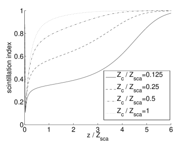
Figure 1: Scintillation index at the beam center (10.8) as a function of the propagation distance for different values of $Z_{\rm sca}$ and $Z_{\rm c}$. Here $\tilde{C}(x)=\exp(-x^{2})$.

In order to get more explicit expressions that facilitate interpretation of the results let us assume that $C({{\itbf x}})$ can be expanded as

$$C({{\itbf x}})=C({\bf 0})-\frac{\gamma}{2}|{{\itbf x}}|^{2}+o(|{{\itbf x}}|^{2}),\quad\quad{{\itbf x}}\to{\bf 0}.$$ (10.9)

When scattering is strong in the sense that the propagation distance is larger than the scattering mean free path $k_{0}^{2}C({\bf 0})z\gg 1$, we have

$$K(z)^{1/2}A(z,{\boldsymbol{\xi}},{\boldsymbol{\zeta}})\simeq\frac{(2\pi)^{4}}{\pi k_{0}^{2}\gamma z}\exp\Big{(}-\frac{\gamma z^{3}}{96}|{\boldsymbol{\zeta}}|^{2}-\frac{2}{k_{0}^{2}\gamma z}|{\boldsymbol{\xi}}|^{2}+\frac{iz}{2k_{0}}{\boldsymbol{\zeta}}\cdot{\boldsymbol{\xi}}\Big{)},$$

and Eqs. (10.3) and (10.5) can be simplified:

$$\Gamma^{(2,{\varepsilon})}(z,{{\itbf r}},{{\itbf q}})\stackrel{{\scriptstyle{\varepsilon}\to 0}}{{\longrightarrow}}\frac{r_{0}^{2}}{r_{0}^{2}+\frac{\gamma z^{3}}{6}}$$

$$\quad\quad\times\exp\Big{(}-\frac{|{{\itbf r}}|^{2}}{r_{0}^{2}+\frac{\gamma z^{3}}{6}}-\frac{k_{0}^{2}\gamma z|{{\itbf q}}|^{2}}{8}\frac{r_{0}^{2}+\frac{\gamma z^{3}}{24}}{r_{0}^{2}+\frac{\gamma z^{3}}{6}}+i\frac{k_{0}\gamma z^{2}{{\itbf r}}\cdot{{\itbf q}}}{4(r_{0}^{2}+\frac{\gamma z^{3}}{6})}\Big{)},$$ (10.10)

$$\Gamma^{(4,{\varepsilon})}(z,{{\itbf r}},{{\itbf q}})\stackrel{{\scriptstyle{\varepsilon}\to 0}}{{\longrightarrow}}\frac{r_{0}^{4}}{\big{(}r_{0}^{2}+\frac{\gamma z^{3}}{6}\big{)}^{2}}$$

$$\quad\quad\times\exp\Big{(}-\frac{2|{{\itbf r}}|^{2}}{r_{0}^{2}+\frac{\gamma z^{3}}{6}}\Big{)}\Big{[}1+\exp\Big{(}-\frac{k_{0}^{2}\gamma z|{{\itbf q}}|^{2}}{4}\frac{r_{0}^{2}+\frac{\gamma z^{3}}{24}}{r_{0}^{2}+\frac{\gamma z^{3}}{6}}\Big{)}\Big{]}.$$ (10.11)

This shows that, in the regime ${\varepsilon}\to 0$ and $k_{0}^{2}C({\bf 0})z\gg 1$:
- The beam radius is $R_{z}$ with

$$R_{z}^{2}:=r_{0}^{2}+\frac{\gamma z^{3}}{6}.$$ (10.12)

- The correlation radius of the intensity distribution is $\rho_{z}$ with

$$\rho_{z}^{2}:=\frac{4}{k_{0}^{2}\gamma z}\frac{r_{0}^{2}+\frac{\gamma z^{3}}{6}}{r_{0}^{2}+\frac{\gamma z^{3}}{24}},$$ (10.13)

which is of the same order as the correlation radius of the field (compare the ${{\itbf q}}$-dependence of (10) and (10.11)).
- The scintillation index is close to one:

$$S^{\varepsilon}(z,{{\itbf r}})=\frac{\Gamma^{(4,{\varepsilon})}(z,{{\itbf r}},{\bf 0})-\Gamma^{(2,{\varepsilon})}(z,{{\itbf r}},{\bf 0})^{2}}{\Gamma^{(2,{\varepsilon})}(z,{{\itbf r}},{\bf 0})^{2}}\simeq 1.$$ (10.14)

This observation is consistent with the physical intuition that, in the strongly scattering regime $z/Z_{\rm sca}\gg 1$, the wave field is conjectured to have zero-mean complex circularly symmetric Gaussian statistics, and therefore the intensity is expected to have exponential (or Rayleigh) distribution [15, 29], in agreement with (10.14).

11 Stability of the Wigner Transform of the Field

The Wigner transform of the transmitted field is defined by

$${W}^{\varepsilon}(z,{{\itbf r}},{\boldsymbol{\xi}}):=\int\exp\big{(}-i{\boldsymbol{\xi}}\cdot{{\itbf q}}\big{)}{u}\big{(}\frac{z}{{\varepsilon}},\frac{{{\itbf r}}}{{\varepsilon}}+\frac{{{\itbf q}}}{2}\big{)}\overline{u}\big{(}\frac{z}{{\varepsilon}},\frac{{{\itbf r}}}{{\varepsilon}}-\frac{{{\itbf q}}}{2}\big{)}d{{\itbf q}}.$$ (11.1)

It is an important quantity that can be interpreted as the angularly-resolved wave energy density (note, however, that it is real-valued but not always non-negative valued). Remember that the initial source is (8.2). This means that the Wigner transform is observed at a mid point ${{\itbf r}}/{\varepsilon}$ that is at the scale of the initial beam radius, while the offset ${{\itbf q}}$ is observed at the scale of the correlation length of the medium. In the homogeneous case, we find

$${W}^{\varepsilon}(z,{{\itbf r}},{\boldsymbol{\xi}})\mid_{\rm homo}=\frac{4\pi r_{0}^{2}}{{\varepsilon}^{2}}\exp\big{(}-\frac{|{\boldsymbol{\xi}}|^{2}r_{0}^{2}}{{\varepsilon}^{2}}-\frac{|{{\itbf r}}-{\boldsymbol{\xi}}z/k_{0}|^{2}}{r_{0}^{2}}\big{)},$$ (11.2)

which is concentrated in a narrow cone in ${\boldsymbol{\xi}}$. Indeed the ${\boldsymbol{\xi}}$-dependence of the Wigner transform reflects the angular diversity of the beam. In the limit ${\varepsilon}\to 0$, we have

$${W}^{\varepsilon}(z,{{\itbf r}},{\boldsymbol{\xi}})\mid_{\rm homo}\stackrel{{\scriptstyle{\varepsilon}\to 0}}{{\longrightarrow}}(2\pi)^{2}\delta({\boldsymbol{\xi}})\exp\big{(}-\frac{|{{\itbf r}}|^{2}}{r_{0}^{2}}\big{)},$$ (11.3)

in the sense that, for any continuous and bounded function $\psi$,

$$\iint{W}^{\varepsilon}(z,{{\itbf r}},{\boldsymbol{\xi}})\mid_{\rm homo}\psi({{\itbf r}},{\boldsymbol{\xi}})d{{\itbf r}}d{\boldsymbol{\xi}}\stackrel{{\scriptstyle{\varepsilon}\to 0}}{{\longrightarrow}}(2\pi)^{2}\int\exp\Big{(}-\frac{|{{\itbf r}}|^{2}}{r_{0}^{2}}\Big{)}\psi({{\itbf r}},{\bf 0})d{{\itbf r}}.$$

In the random case, the ${\boldsymbol{\xi}}$-dependence of the Wigner transform depends on the angular diversity of the initial beam but also on the scattering by the random medium, which dramatically broadens it because the correlation length of the medium is smaller than the initial beam width. As a result (see (6.4) with $r_{0}\to r_{0}/{\varepsilon}$, $z\to z/{\varepsilon}$, and $C\to{\varepsilon}C$), the expectation of the Wigner transform is:

$$\mathbb{E}[{W}^{\varepsilon}(z,{{\itbf r}},{\boldsymbol{\xi}})] = \frac{r_{0}^{2}}{4\pi{\varepsilon}^{2}}\iint\exp\Big{(}-\frac{r_{0}^{2}|{\boldsymbol{\zeta}}|^{2}}{4{\varepsilon}^{2}}-\frac{{\varepsilon}^{2}|{{\itbf q}}|^{2}}{4r_{0}^{2}}+i\frac{{\boldsymbol{\zeta}}}{{\varepsilon}}\cdot\big{(}{{\itbf r}}-\frac{{\boldsymbol{\xi}}z}{k_{0}}\big{)}-i{\boldsymbol{\xi}}\cdot{{\itbf q}}\Big{)}$$ (11.4)

$$\times\exp\Big{(}\frac{k_{0}^{2}{\varepsilon}}{4}\int_{0}^{z/{\varepsilon}}C\big{(}{{\itbf q}}+{\boldsymbol{\zeta}}\frac{z^{\prime}}{k_{0}}\big{)}-C({\bf 0})dz^{\prime}\Big{)}d{\boldsymbol{\zeta}}d{{\itbf q}}$$

$$= \frac{r_{0}^{2}}{4\pi}\iint\exp\Big{(}-\frac{r_{0}^{2}|{\boldsymbol{\zeta}}|^{2}}{4}-\frac{{\varepsilon}^{2}|{{\itbf q}}|^{2}}{4r_{0}^{2}}+i{\boldsymbol{\zeta}}\cdot\big{(}{{\itbf r}}-\frac{{\boldsymbol{\xi}}z}{k_{0}}\big{)}-i{\boldsymbol{\xi}}\cdot{{\itbf q}}\Big{)}$$

$$\times\exp\Big{(}\frac{k_{0}^{2}}{4}\int_{0}^{z}C\big{(}{{\itbf q}}+{\boldsymbol{\zeta}}\frac{z^{\prime}}{k_{0}}\big{)}-C({\bf 0})dz^{\prime}\Big{)}d{\boldsymbol{\zeta}}d{{\itbf q}},$$

so that in the limit ${\varepsilon}\to 0$ it is given by

$$\mathbb{E}[{W}^{\varepsilon}(z,{{\itbf r}},{\boldsymbol{\xi}})] \stackrel{{\scriptstyle{\varepsilon}\to 0}}{{\longrightarrow}} \frac{r_{0}^{2}}{4\pi}\iint\exp\Big{(}-\frac{r_{0}^{2}|{\boldsymbol{\zeta}}|^{2}}{4}+i{\boldsymbol{\zeta}}\cdot{{\itbf r}}-i{\boldsymbol{\xi}}\cdot\big{(}{{\itbf q}}+{\boldsymbol{\zeta}}\frac{z}{k_{0}}\big{)}\Big{)}$$ (11.5)

$$\times\exp\Big{(}\frac{k_{0}^{2}}{4}\int_{0}^{z}C\big{(}{{\itbf q}}+{\boldsymbol{\zeta}}\frac{z^{\prime}}{k_{0}}\big{)}-C({\bf 0})dz^{\prime}\Big{)}d{\boldsymbol{\zeta}}d{{\itbf q}}.$$

More precisely, the mean Wigner transform can be split into two pieces: a narrow cone and a broad cone in ${\boldsymbol{\xi}}$:

$$\mathbb{E}[{W}^{\varepsilon}(z,{{\itbf r}},{\boldsymbol{\xi}})]\stackrel{{\scriptstyle{\varepsilon}\to 0}}{{\longrightarrow}}\frac{K(z)^{1/2}}{(2\pi)^{2}}\delta({\boldsymbol{\xi}})\exp\Big{(}-\frac{|{{\itbf r}}|^{2}}{r_{0}^{2}}\Big{)}$$

$$\quad\quad+\frac{r_{0}^{2}K(z)^{1/2}}{(2\pi)^{3}}\int\exp\Big{(}-\frac{r_{0}^{2}|{\boldsymbol{\zeta}}|^{2}}{4}+i{\boldsymbol{\zeta}}\cdot\big{(}{{\itbf r}}-{\boldsymbol{\xi}}\frac{z}{k_{0}}\big{)}\Big{)}A(z,{\boldsymbol{\xi}},{\boldsymbol{\zeta}})d{\boldsymbol{\zeta}}.$$ (11.6)

The narrow cone is the contribution of the coherent transmitted wave components and it decays exponentially with the propagation distance (see the expression (8.9) for $K(z)$). The broad cone is the contributions of the incoherent scattered waves and it becomes dominant when the propagation distance becomes so large that $k_{0}^{2}C({\bf 0})z\gg 1$.

It is known that the Wigner transform is not statistically stable, and that it is necessary to smooth it (that is to say, to convolve it with a kernel) to get a quantity that can be measured in a statistically stable way (that is to say, the Wigner transform for one typical realization is approximately equal to its expected value) [3, 39]. Our goal in this section is to quantify this statistical stability.

Let us consider two positive parameters $r_{\rm s}$ and $\xi_{\rm s}$ and define the smoothed Wigner transform:

$${W}^{\varepsilon}_{\rm s}(z,{{\itbf r}},{\boldsymbol{\xi}})=\frac{1}{(2\pi)^{2}{\varepsilon}^{2}r_{\rm s}^{2}\xi_{\rm s}^{2}}\iint{W}^{\varepsilon}(z,{{\itbf r}}-{{\itbf r}}^{\prime},{\boldsymbol{\xi}}-{\boldsymbol{\xi}}^{\prime})\exp\Big{(}-\frac{|{{\itbf r}}^{\prime}|^{2}}{2{\varepsilon}^{2}r_{\rm s}^{2}}-\frac{|{\boldsymbol{\xi}}^{\prime}|^{2}}{2\xi_{\rm s}^{2}}\Big{)}d{{\itbf r}}^{\prime}d{\boldsymbol{\xi}}^{\prime}.$$ (11.7)

In view of the form of the Wigner transform in the homogeneous case in (11.2) this is indeed the natural scales at which to smooth. The expectation of the smoothed Wigner transform is in the limit ${\varepsilon}\to 0$:

$$\mathbb{E}\big{[}{W}^{\varepsilon}_{\rm s}(z,{{\itbf r}},{\boldsymbol{\xi}})\big{]} \stackrel{{\scriptstyle{\varepsilon}\to 0}}{{\longrightarrow}} \frac{r_{0}^{2}}{4\pi}\iint\exp\Big{(}-\frac{r_{0}^{2}|{\boldsymbol{\zeta}}|^{2}}{4}-\frac{\xi_{\rm s}^{2}|{{\itbf q}}+{\boldsymbol{\zeta}}\frac{z}{k_{0}}|^{2}}{2}-i{\boldsymbol{\xi}}\cdot\big{(}{{\itbf q}}+{\boldsymbol{\zeta}}\frac{z}{k_{0}}\big{)}\Big{)}$$ (11.8)

$$\times\exp\Big{(}i{\boldsymbol{\zeta}}\cdot{{\itbf r}}+\frac{k_{0}^{2}}{4}\int_{0}^{z}C\big{(}{{\itbf q}}+{\boldsymbol{\zeta}}\frac{z^{\prime}}{k_{0}}\big{)}-C({\bf 0})dz^{\prime}\Big{)}d{\boldsymbol{\zeta}}d{{\itbf q}}.$$

It can also be written as follows.

Proposition 11.1.

Under Hypothesis (2.5), the expectation of the smoothed Wigner transform (11.7) satisfies, in the scintillation regime ${\varepsilon}\to 0$:

$$\mathbb{E}\big{[}{W}^{\varepsilon}_{\rm s}(z,{{\itbf r}},{\boldsymbol{\xi}})\big{]} \stackrel{{\scriptstyle{\varepsilon}\to 0}}{{\longrightarrow}} \frac{K(z)^{1/2}}{(2\pi)^{3}\xi_{\rm s}^{2}}\exp\Big{(}-\frac{|{\boldsymbol{\xi}}|^{2}}{2\xi_{\rm s}^{2}}\Big{)}\exp\Big{(}-\frac{|{{\itbf r}}|^{2}}{r_{0}^{2}}\Big{)}$$ (11.9)

$$+\frac{K(z)^{1/2}r_{0}^{2}}{(2\pi)^{4}\xi_{\rm s}^{2}}\iint A(z,{\boldsymbol{\xi}}^{\prime},{\boldsymbol{\zeta}})\exp\Big{(}-\frac{r_{0}^{2}|{\boldsymbol{\zeta}}|^{2}}{4}-\frac{|{\boldsymbol{\xi}}^{\prime}-{\boldsymbol{\xi}}|^{2}}{2\xi_{\rm s}^{2}}+i{\boldsymbol{\zeta}}\cdot\big{(}{{\itbf r}}-{\boldsymbol{\xi}}^{\prime}\frac{z}{k_{0}}\big{)}\Big{)}d{\boldsymbol{\zeta}}d{\boldsymbol{\xi}}^{\prime},\hskip 21.68121pt$$

where $K$ and $A$ are defined by (8.9) and (8.10).

The first term in (11.9) is a narrow cone in ${\boldsymbol{\xi}}$ around ${\boldsymbol{\xi}}={\bf 0}$ corresponding to coherent wave components and the second term is a broad cone in ${\boldsymbol{\xi}}$ corresponding to incoherent wave components. Note that the expectation of the smoothed Wigner transform is independent on $r_{\rm s}$ as the smoothing in ${{\itbf r}}$ vanishes in the limit ${\varepsilon}\to 0$. However the smoothing in ${{\itbf r}}$ plays an important role in the control of the fluctuations of the Wigner transform. We will analyze the variance of the smoothed Wigner transform and its dependence on the smoothing parameters $r_{\rm s}$ and $\xi_{\rm s}$.

The second moment of the smoothed Wigner transform is

$$\mathbb{E}[{W}^{\varepsilon}_{\rm s}(z,{{\itbf r}},{\boldsymbol{\xi}})^{2}]=\frac{1}{(2\pi)^{2}{\varepsilon}^{4}r_{\rm s}^{4}}\iint\exp\Big{(}-\frac{|{{\itbf r}}_{\rm s}|^{2}+|{{\itbf r}}_{\rm s}^{\prime}|^{2}}{2{\varepsilon}^{2}r_{\rm s}^{2}}-\frac{\xi_{\rm s}^{2}(|{{\itbf q}}|^{2}+|{{\itbf q}}^{\prime}|^{2})}{2}\Big{)}$$

$$\quad\times\mu\Big{(}\frac{z}{{\varepsilon}},\frac{{{\itbf q}}+{{\itbf q}}^{\prime}}{2},\frac{{{\itbf q}}-{{\itbf q}}^{\prime}}{2},\frac{2{{\itbf r}}+{{\itbf r}}_{\rm s}+{{\itbf r}}_{\rm s}^{\prime}}{{\varepsilon}},\frac{{{\itbf r}}_{\rm s}-{{\itbf r}}_{\rm s}^{\prime}}{{\varepsilon}}\Big{)}$$

$$\quad\times\exp\big{(}-i{\boldsymbol{\xi}}\cdot({{\itbf q}}+{{\itbf q}}^{\prime})\big{)}d{{\itbf q}}d{{\itbf q}}^{\prime}d{{\itbf r}}_{\rm s}d{{\itbf r}}_{\rm s}^{\prime},$$

which gives, using (8.3), (7.6), and (7.8):

$$\mathbb{E}\big{[}{W}^{\varepsilon}_{\rm s}(z,{{\itbf r}},{\boldsymbol{\xi}})^{2}\big{]}=\frac{1}{(2\pi)^{6}\xi_{\rm s}^{4}}\iint\exp\Big{(}-r_{\rm s}^{2}|{\boldsymbol{\zeta}}_{1}|^{2}-r_{\rm s}^{2}|{\boldsymbol{\zeta}}_{2}|^{2}-\frac{|{\boldsymbol{\xi}}_{1}-2{\boldsymbol{\xi}}|^{2}}{4\xi_{\rm s}^{2}}-\frac{|{\boldsymbol{\xi}}_{2}|^{2}}{4\xi_{\rm s}^{2}}\Big{)}$$

$$\quad\times\exp\Big{(}2i\frac{{\boldsymbol{\zeta}}_{1}\cdot{{\itbf r}}}{{\varepsilon}}-i\frac{z}{k_{0}{\varepsilon}}\big{(}{\boldsymbol{\zeta}}_{1}\cdot{\boldsymbol{\xi}}_{1}+{\boldsymbol{\zeta}}_{2}\cdot{\boldsymbol{\xi}}_{2}\big{)}\Big{)}\tilde{\mu}^{\varepsilon}(z,{\boldsymbol{\xi}}_{1},{\boldsymbol{\xi}}_{2},{\boldsymbol{\zeta}}_{1},{\boldsymbol{\zeta}}_{2})d{\boldsymbol{\zeta}}_{1}d{\boldsymbol{\zeta}}_{2}d{\boldsymbol{\xi}}_{1}d{\boldsymbol{\xi}}_{2}.$$

Using Proposition 8.1 and the fact that $A(z,-{\boldsymbol{\xi}},-{\boldsymbol{\zeta}})=A(z,{\boldsymbol{\xi}},{\boldsymbol{\zeta}})$, we get the following proposition.

Proposition 11.2.

Under Hypothesis (2.5), the second moment of the smoothed Wigner transform (11.7) is, in the scintillation regime ${\varepsilon}\to 0$:

$$\mathbb{E}\big{[}{W}^{\varepsilon}_{\rm s}(z,{{\itbf r}},{\boldsymbol{\xi}})^{2}\big{]}\stackrel{{\scriptstyle{\varepsilon}\to 0}}{{\longrightarrow}}\frac{K(z)}{(2\pi)^{6}\xi_{\rm s}^{4}}\exp\Big{(}-\frac{|{\boldsymbol{\xi}}|^{2}}{\xi_{\rm s}^{2}}\Big{)}\exp\Big{(}-\frac{2|{{\itbf r}}|^{2}}{r_{0}^{2}}\Big{)}$$

$$+\frac{r_{0}^{4}K(z)}{(2\pi)^{8}\xi_{\rm s}^{4}}\iint d{\boldsymbol{\xi}}_{1}d{\boldsymbol{\zeta}}_{1}e^{i{\boldsymbol{\zeta}}_{1}\cdot(2{{\itbf x}}-\frac{z}{k_{0}}{\boldsymbol{\xi}}_{1})-\frac{r_{0}^{2}|{\boldsymbol{\zeta}}_{1}|^{2}}{2}-\frac{|{\boldsymbol{\xi}}_{1}-2{\boldsymbol{\xi}}|^{2}}{4\xi_{\rm s}^{2}}}$$

$$\times\bigg{\{}4e^{-\frac{|{\boldsymbol{\xi}}_{1}|^{2}}{4\xi_{\rm s}^{2}}}\int e^{-i\frac{z}{k_{0}}{\boldsymbol{\xi}}_{1}\cdot{\boldsymbol{\zeta}}_{2}-\frac{r_{0}^{2}|{\boldsymbol{\zeta}}_{2}|^{2}}{2}}A(z,{\boldsymbol{\xi}}_{1},{\boldsymbol{\zeta}}_{2}+{\boldsymbol{\zeta}}_{1})d{\boldsymbol{\zeta}}_{2}$$

$$+\iint e^{-\frac{|{\boldsymbol{\xi}}_{2}|^{2}}{4\xi_{\rm s}^{2}}-i\frac{z}{k_{0}}{\boldsymbol{\xi}}_{2}\cdot{\boldsymbol{\zeta}}_{2}-\frac{r_{0}^{2}|{\boldsymbol{\zeta}}_{2}|^{2}}{2}}A\big{(}z,\frac{{\boldsymbol{\xi}}_{2}+{\boldsymbol{\xi}}_{1}}{2},{\boldsymbol{\zeta}}_{2}+{\boldsymbol{\zeta}}_{1}\big{)}$$

$$\hskip 79.49744pt\times A\big{(}z,\frac{{\boldsymbol{\xi}}_{2}-{\boldsymbol{\xi}}_{1}}{2},{\boldsymbol{\zeta}}_{2}-{\boldsymbol{\zeta}}_{1}\big{)}d{\boldsymbol{\xi}}_{2}d{\boldsymbol{\zeta}}_{2}$$

$$+4e^{-r_{\rm s}^{2}|{\boldsymbol{\xi}}_{1}|^{2}}\int e^{-i\frac{z}{k_{0}}{\boldsymbol{\xi}}_{1}\cdot{\boldsymbol{\xi}}_{2}-\frac{r_{0}^{2}|{\boldsymbol{\xi}}_{2}|^{2}}{2}}A(z,{\boldsymbol{\xi}}_{1},{\boldsymbol{\xi}}_{2}+{\boldsymbol{\zeta}}_{1})d{\boldsymbol{\xi}}_{2}$$

$$+\iint e^{-r_{\rm s}^{2}|{\boldsymbol{\zeta}}_{2}|^{2}-i\frac{z}{k_{0}}{\boldsymbol{\xi}}_{2}\cdot{\boldsymbol{\zeta}}_{2}-\frac{r_{0}^{2}|{\boldsymbol{\xi}}_{2}|^{2}}{2}}A\big{(}z,\frac{{\boldsymbol{\zeta}}_{2}+{\boldsymbol{\xi}}_{1}}{2},{\boldsymbol{\xi}}_{2}+{\boldsymbol{\zeta}}_{1}\big{)}$$

$$\hskip 79.49744pt\times A\big{(}z,\frac{{\boldsymbol{\zeta}}_{2}-{\boldsymbol{\xi}}_{1}}{2},{\boldsymbol{\xi}}_{2}-{\boldsymbol{\zeta}}_{1}\big{)}d{\boldsymbol{\xi}}_{2}d{\boldsymbol{\zeta}}_{2}\bigg{\}}.$$ (11.10)

This is an exact expression but, as it involves four-dimensional integrals, it is complicated to interpret it. This expression becomes simple in the strongly scattering regime $k_{0}^{2}C({\bf 0})z\gg 1$, because then $A(z,{\boldsymbol{\xi}},{\boldsymbol{\zeta}})$ takes a Gaussian form and all integrals can be evaluated. To get more explicit expressions in the discussion of the results we here again assume that $C({{\itbf x}})$ can be expanded as (10.9). When $k_{0}^{2}C({\bf 0})z\gg 1$, we have

$$\mathbb{E}\big{[}{W}^{\varepsilon}_{\rm s}(z,{{\itbf r}},{\boldsymbol{\xi}})\big{]} \stackrel{{\scriptstyle{\varepsilon}\to 0}}{{\longrightarrow}} \frac{8\pi}{k_{0}^{2}\gamma z}\frac{r_{0}^{2}}{(r_{0}^{2}+\frac{\gamma z^{3}}{24})(1+\frac{4\xi_{\rm s}^{2}}{k_{0}^{2}\gamma z})+\frac{z^{2}\xi_{\rm s}^{2}}{2k_{0}^{2}}}$$ (11.11)

$$\times\exp\bigg{(}-\frac{\Big{|}{{\itbf r}}-\frac{z{\boldsymbol{\xi}}}{2k_{0}(1+\frac{4\xi_{\rm s}^{2}}{k_{0}^{2}\gamma z})}\Big{|}^{2}}{r_{0}^{2}+\frac{\gamma z^{3}}{24}+\frac{\frac{z^{2}\xi_{\rm s}^{2}}{2k_{0}^{2}}}{1+\frac{4\xi_{\rm s}^{2}}{k_{0}^{2}\gamma z}}}-\frac{2|{\boldsymbol{\xi}}|^{2}}{k_{0}^{2}\gamma z+4\xi_{\rm s}^{2}}\bigg{)}$$

and

$$\mathbb{E}\big{[}{W}^{\varepsilon}_{\rm s}(z,{{\itbf r}},{\boldsymbol{\xi}})^{2}\big{]} \stackrel{{\scriptstyle{\varepsilon}\to 0}}{{\longrightarrow}} \lim_{{\varepsilon}\to 0}\mathbb{E}\big{[}{W}^{\varepsilon}_{\rm s}(z,{{\itbf r}},{\boldsymbol{\xi}})\big{]}^{2}\left(1+\frac{(r_{0}^{2}+\frac{\gamma z^{3}}{24})(1+\frac{4\xi_{\rm s}^{2}}{k_{0}^{2}\gamma z})+\frac{z^{2}\xi_{\rm s}^{2}}{2k_{0}^{2}}}{(r_{0}^{2}+\frac{\gamma z^{3}}{24})(4r_{\rm s}^{2}\xi_{\rm s}^{2}+\frac{4\xi_{\rm s}^{2}}{k_{0}^{2}\gamma z})+\frac{z^{2}\xi_{\rm s}^{2}}{2k_{0}^{2}}}\right).$$

The coefficient of variation ${C}^{\varepsilon}_{\rm s}$ of the smoothed Wigner transform is defined by:

$${C}_{\rm s}^{\varepsilon}(z,{{\itbf r}},{\boldsymbol{\xi}}):=\frac{\sqrt{\mathbb{E}[{W}^{\varepsilon}_{\rm s}(z,{{\itbf r}},{\boldsymbol{\xi}})^{2}]-\mathbb{E}[{W}^{\varepsilon}_{\rm s}(z,{{\itbf r}},{\boldsymbol{\xi}})]^{2}}}{\mathbb{E}[{W}^{\varepsilon}_{\rm s}(z,{{\itbf r}},{\boldsymbol{\xi}})]}.$$ (11.12)

We then get the following expression for the coefficient of variation in the strongly scattering regime $k_{0}^{2}C({\bf 0})z\gg 1$.

Corollary 11.3.

Under the same hypotheses as in Propositions 11.1 and 11.2, if additionally $k_{0}^{2}C({\bf 0})z\gg 1$ and $C$ can be expanded as (10.9), then the coefficient of variation of the smoothed Wigner transform (11.7) satisfies

$${C}^{\varepsilon}_{\rm s}(z,{{\itbf r}},{\boldsymbol{\xi}})\stackrel{{\scriptstyle{\varepsilon}\to 0}}{{\longrightarrow}}\left(\frac{(r_{0}^{2}+\frac{\gamma z^{3}}{24})(1+\frac{4\xi_{\rm s}^{2}}{k_{0}^{2}\gamma z})+\frac{z^{2}\xi_{\rm s}^{2}}{2k_{0}^{2}}}{(r_{0}^{2}+\frac{\gamma z^{3}}{24})(4r_{\rm s}^{2}\xi_{\rm s}^{2}+\frac{4\xi_{\rm s}^{2}}{k_{0}^{2}\gamma z})+\frac{z^{2}\xi_{\rm s}^{2}}{2k_{0}^{2}}}\right)^{1/2}=\left(\frac{\frac{1}{\xi_{\rm s}^{2}\rho_{z}^{2}}+1}{\frac{4r_{\rm s}^{2}}{\rho_{z}^{2}}+1}\right)^{1/2},$$ (11.13)

where $\rho_{z}$ is the correlation radius (10.13).

Note that the coefficient of variation becomes independent of ${{\itbf r}}$ and ${\boldsymbol{\xi}}$. Eq. (11.13) is a simple enough formula to help determining the smoothing parameters $\xi_{\rm s}$ and $r_{\rm s}$ that are needed to reach a given value for the coefficient of variation. The coefficient of variation is plotted in Figure 2, which exhibits the line $2\xi_{\rm s}r_{\rm s}=1$ separating the two regions where the coefficient of variation is larger or smaller than one.

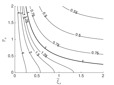
Figure 2: Contour levels of the coefficient of variation (11.13) of the smoothed Wigner transform. Here $\overline{r}_{\rm s}=r_{\rm s}/\rho_{z}$ and $\overline{\xi}_{\rm s}=\xi_{\rm s}\rho_{z}$. The contour level $1$ is $2\overline{\xi}_{\rm s}\overline{r}_{\rm s}=1$.

For $2\xi_{\rm s}r_{\rm s}=1$, we have $\lim_{{\varepsilon}\to 0}{C}^{\varepsilon}_{\rm s}(z,{{\itbf r}},{\boldsymbol{\xi}})=1$. For $2\xi_{\rm s}r_{\rm s}<1$ (resp. $>1$) we have $\lim_{{\varepsilon}\to 0}{C}^{\varepsilon}_{\rm s}(z,{{\itbf r}},{\boldsymbol{\xi}})>1$ (resp. $<1$). The curve $2\xi_{\rm s}r_{\rm s}=1$ determines the region where the coefficient of variation of ${W}^{\varepsilon}_{\rm s}(z,{{\itbf r}},{\boldsymbol{\xi}})$ is smaller or larger than one (in the limit ${\varepsilon}\to 0$). The critical value $r_{\rm s}=1/(2\xi_{\rm s})$ is indeed special. In this case, the smoothed Wigner transform (11.7) can be written as the double convolution of the Wigner transform $W^{\varepsilon}$ of the random field $u(\frac{z}{{\varepsilon}},\cdot)$ with the Wigner transform

$$W^{\varepsilon}_{\rm g}({{\itbf r}},{\boldsymbol{\xi}}):=\int\exp\big{(}-i{\boldsymbol{\xi}}\cdot{{\itbf q}}\big{)}u_{\rm g}\big{(}\frac{{{\itbf r}}}{{\varepsilon}}+\frac{{{\itbf q}}}{2}\big{)}\overline{u_{\rm g}}\big{(}\frac{{{\itbf r}}}{{\varepsilon}}-\frac{{{\itbf q}}}{2}\big{)}d{{\itbf q}}$$

of the Gaussian state

$$u_{\rm g}({{\itbf x}}):=\exp\big{(}-\xi_{\rm s}^{2}|{{\itbf x}}|^{2}\big{)},$$

since we have

$${W}^{\varepsilon}_{\rm g}({{\itbf r}},{\boldsymbol{\xi}})=\frac{2\pi}{\xi_{\rm s}^{2}}\exp\Big{(}-2\frac{\xi_{\rm s}^{2}|{{\itbf r}}|^{2}}{{\varepsilon}^{2}}-\frac{|{\boldsymbol{\xi}}|^{2}}{2\xi_{\rm s}^{2}}\Big{)},$$

and therefore

$${W}^{\varepsilon}_{\rm s}(z,{{\itbf r}},{\boldsymbol{\xi}})=\frac{4\xi_{\rm s}^{2}}{(2\pi)^{3}{\varepsilon}^{2}}\iint W^{\varepsilon}(z,{{\itbf r}}-{{\itbf r}}^{\prime},{\boldsymbol{\xi}}-{\boldsymbol{\xi}}^{\prime})W^{\varepsilon}_{\rm g}({{\itbf r}}^{\prime},{\boldsymbol{\xi}}^{\prime})d{{\itbf r}}^{\prime}d{\boldsymbol{\xi}}^{\prime},$$

for $r_{\rm s}=1/(2\xi_{\rm s})$. It is known that the convolution of a Wigner transform with a kernel that is itself the Wigner transform of a function (such as a Gaussian) is nonnegative real valued (the smoothed Wigner transform obtained with the Gaussian $W^{\varepsilon}_{\rm g}$ is sometimes called Husimi function) [6, 34]. This can be shown easily in our case as the smoothed Wigner transform can be written as

$${W}^{\varepsilon}_{\rm s}(z,{{\itbf r}},{\boldsymbol{\xi}})=\frac{2\xi_{\rm s}^{2}}{\pi}\Big{|}\int\exp\big{(}i{{\boldsymbol{\xi}}\cdot{{\itbf r}}^{\prime}}\big{)}\overline{u_{\rm g}}\big{(}{{\itbf r}}^{\prime}\big{)}u\big{(}\frac{z}{{\varepsilon}},\frac{{{\itbf r}}}{{\varepsilon}}-{{\itbf r}}^{\prime}\big{)}d{{\itbf r}}^{\prime}\Big{|}^{2},$$ (11.14)

for $r_{\rm s}=1/(2\xi_{\rm s})$. From this representation formula of ${W}^{\varepsilon}_{\rm s}$ valid for $r_{\rm s}=1/(2\xi_{\rm s})$, we can see that it is the square modulus of a linear functional of $u(\frac{z}{{\varepsilon}},\cdot)$. The physical intuition that $u(\frac{z}{{\varepsilon}},\cdot)$ has circularly symmetric complex Gaussian statistics in strongly scattering media then predicts that ${W}^{\varepsilon}_{\rm s}(z,{{\itbf r}},{\boldsymbol{\xi}})$ should have an exponential (or Rayleigh) distribution, because the sum of the squares of two independent real-valued Gaussian random variables has an exponential distribution. This is indeed consistent with our theoretical finding that $\lim_{{\varepsilon}\to 0}{C}^{\varepsilon}_{\rm s}=1$ for $r_{\rm s}=1/(2\xi_{\rm s})$. In fact the situation with complex scattering giving a field that has centered circularly symmetric Gaussian statistics is exactly what motivates the name “scintillation regime” with unit relative intensity fluctuations.

If $r_{\rm s}>1/(2\xi_{\rm s})$, by observing that

$$\exp\Big{(}-\frac{|{{\itbf r}}|^{2}}{2{\varepsilon}^{2}r_{\rm s}^{2}}\Big{)}=\Psi^{\varepsilon}({{\itbf r}})*_{{\itbf r}}\exp\Big{(}-\frac{2\xi_{\rm s}^{2}|{{\itbf r}}|^{2}}{{\varepsilon}^{2}}\Big{)},$$

where $*_{{\itbf r}}$ stands for the convolution product in ${{\itbf r}}$:

$$\Psi^{\varepsilon}({{\itbf r}})*_{{\itbf r}}f({{\itbf r}})=\int\Psi^{\varepsilon}({{\itbf r}}-{{\itbf r}}^{\prime})f({{\itbf r}}^{\prime})d{{\itbf r}}^{\prime},$$

and the function $\Psi^{\varepsilon}$ is defined by

$$\Psi^{\varepsilon}({{\itbf r}}):=\frac{8\xi_{\rm s}^{4}r_{\rm s}^{2}}{\pi{\varepsilon}^{2}(4\xi_{\rm s}^{2}r_{\rm s}^{2}-1)}\exp\Big{(}-\frac{2\xi_{\rm s}^{2}|{{\itbf r}}|^{2}}{(4\xi_{\rm s}^{2}r_{\rm s}^{2}-1){\varepsilon}^{2}}\Big{)},$$

we observe that the smoothed Wigner transform (11.7) can be expressed as:

$${W}^{\varepsilon}_{\rm s}(z,{{\itbf r}},{\boldsymbol{\xi}})=\Psi^{\varepsilon}({{\itbf r}})*_{{\itbf r}}\left(\frac{2\xi_{\rm s}^{2}}{\pi}\Big{|}\int\exp\big{(}i{{\boldsymbol{\xi}}\cdot{{\itbf r}}^{\prime}}\big{)}\overline{u_{\rm g}}\big{(}{{\itbf r}}^{\prime}\big{)}u\big{(}\frac{z}{{\varepsilon}},\frac{{{\itbf r}}}{{\varepsilon}}-{{\itbf r}}^{\prime}\big{)}d{{\itbf r}}^{\prime}\Big{|}^{2}\right),$$ (11.15)

for $r_{\rm s}>1/(2\xi_{\rm s})$. From this representation formula for ${W}^{\varepsilon}_{\rm s}$ valid for $r_{\rm s}>1/(2\xi_{\rm s})$, we can see that it is nonnegative valued and that it is a local average of (11.14), which has a unit coefficient of variation in the strongly scattering scintillation regime. That is why the coefficient of variation of the smoothed Wigner transform is smaller than one when $r_{\rm s}>1/(2\xi_{\rm s})$.

Finally, it is possible to take $r_{\rm s}=0$ in (11.7), which corresponds to the absence of smoothing in ${{\itbf r}}$:

$${W}^{\varepsilon}_{\rm s}(z,{{\itbf r}},{\boldsymbol{\xi}})=\frac{1}{2\pi\xi_{\rm s}^{2}}\int W^{\varepsilon}(z,{{\itbf r}},{\boldsymbol{\xi}}-{\boldsymbol{\xi}}^{\prime})\exp\Big{(}-\frac{|{\boldsymbol{\xi}}^{\prime}|^{2}}{2\xi_{\rm s}^{2}}\Big{)}d{\boldsymbol{\xi}}^{\prime},$$

for $r_{\rm s}=0$. We then get

$${\rm Var}\big{(}{W}^{\varepsilon}_{\rm s}(z,{{\itbf r}},{\boldsymbol{\xi}})\big{)} \stackrel{{\scriptstyle{\varepsilon}\to 0}}{{\longrightarrow}} \frac{\left(\frac{8\pi r_{0}^{2}}{k_{0}^{2}\gamma z}\right)^{2}}{\left((r_{0}^{2}+\frac{\gamma z^{3}}{24})(1+\frac{4\xi_{\rm s}^{2}}{k_{0}^{2}\gamma z})+\frac{z^{2}\xi_{\rm s}^{2}}{2k_{0}^{2}}\right)\left((r_{0}^{2}+\frac{\gamma z^{3}}{24})(\frac{4\xi_{\rm s}^{2}}{k_{0}^{2}\gamma z})+\frac{z^{2}\xi_{\rm s}^{2}}{2k_{0}^{2}}\right)}$$

$$\times\exp\bigg{(}-\frac{2\Big{|}{{\itbf r}}-\frac{z{\boldsymbol{\xi}}}{2k_{0}(1+\frac{4\xi_{\rm s}^{2}}{k_{0}^{2}\gamma z})}\Big{|}^{2}}{r_{0}^{2}+\frac{\gamma z^{3}}{24}+\frac{\frac{z^{2}\xi_{\rm s}^{2}}{2k_{0}^{2}}}{1+\frac{4\xi_{\rm s}^{2}}{k_{0}^{2}\gamma z}}}-\frac{4|{\boldsymbol{\xi}}|^{2}}{k_{0}^{2}\gamma z+4\xi_{\rm s}^{2}}\bigg{)}$$

and

$${C}^{\varepsilon}_{\rm s}(z,{{\itbf r}},{\boldsymbol{\xi}})\stackrel{{\scriptstyle{\varepsilon}\to 0}}{{\longrightarrow}}\sqrt{1+(\xi_{\rm s}\rho_{z})^{-2}},$$

for $r_{\rm s}=0$. If, additionally, we let $\xi_{\rm s}\to\infty$, then we find

$$\lim_{\xi_{\rm s}\to\infty}\lim_{{\varepsilon}\to 0}\frac{\xi_{\rm s}^{2}}{2\pi}\mathbb{E}\big{[}{W}^{\varepsilon}_{\rm s}(z,{{\itbf r}},{\boldsymbol{\xi}})\big{]}=\frac{r_{0}^{2}}{r_{0}^{2}+\frac{\gamma z^{3}}{6}}\exp\Big{(}-\frac{|{{\itbf r}}|^{2}}{r_{0}^{2}+\frac{\gamma z^{3}}{6}}\Big{)},$$

$$\lim_{\xi_{\rm s}\to\infty}\lim_{{\varepsilon}\to 0}\Big{(}\frac{\xi_{\rm s}^{2}}{2\pi}\Big{)}^{2}{\rm Var}\big{(}{W}^{\varepsilon}_{\rm s}(z,{{\itbf r}},{\boldsymbol{\xi}})\big{)}=\Big{(}\frac{r_{0}^{2}}{r_{0}^{2}+\frac{\gamma z^{3}}{6}}\Big{)}^{2}\exp\Big{(}-\frac{2|{{\itbf r}}|^{2}}{r_{0}^{2}+\frac{\gamma z^{3}}{6}}\Big{)},$$

and also

$$\lim_{\xi_{\rm s}\to\infty}\lim_{{\varepsilon}\to 0}{C}^{\varepsilon}_{\rm s}(z,{{\itbf r}},{\boldsymbol{\xi}})=1,$$

for $r_{\rm s}=0$. These results are consistent with formulas (10-10.11) (with ${{\itbf q}}={\bf 0}$) and the fact that

$$\big{|}{u}\big{(}\frac{z}{{\varepsilon}},\frac{{{\itbf r}}}{{\varepsilon}}\big{)}\big{|}^{2}=\frac{1}{(2\pi)^{2}}\int W^{\varepsilon}(z,{{\itbf r}},{\boldsymbol{\xi}}^{\prime})d{\boldsymbol{\xi}}^{\prime}=\lim_{\xi_{\rm s}\to\infty}\frac{\xi_{\rm s}^{2}}{2\pi}{W}^{\varepsilon}_{\rm s}(z,{{\itbf r}},{\boldsymbol{\xi}})\mid_{r_{\rm s}=0}.$$

This shows that the limits $\xi_{\rm s}\to\infty$ and ${\varepsilon}\to 0$ are exchangeable.

12 Conclusions

In this paper we have considered the white-noise paraxial wave model and computed the second and fourth-order moments of the field. In the regime in which the correlation length of the medium is smaller than the initial beam width, the moments exhibit a multi-scale behavior with components varying at these two scales. Our novel characterization of the solution of the fourth-order moment equation allows us to solve important questions: in this paper we have proved that the fourth-order centered moment of the field satisfies the Gaussian summation rule, we analyzed the correlation function of the intensity distribution, and we have computed the variance of the smoothed Wigner transform of the transmitted field. In particular we have characterized quantitatively the amount of smoothing necessary to get a statistically stable smoothed Wigner transform. We believe that our main result can find many other applications, for instance for the stability of time-reversal experiments [5, 38] or the stability of correlation-based imaging techniques in the paraxial regime [10, 11].

Appendix A The Scintillation Regime for the Wave Equation

In Section 8 we address a scaling regime which can be considered as a particular case of the paraxial white-noise regime: the scintillation regime. This corresponds to a situation in which the relative intensity fluctuations are of order one and it is an important regime to capture from the physical viewpoint. We explain in this appendix the conditions for the validity of this regime in the context of the wave equation (2.1).

Let $\sigma$ be the standard deviation of the fluctuations of the index of refraction $n$ in (2.1). Moreover, let $l_{\rm c}$ be the correlation length of the fluctuations of the index of refraction, $\lambda_{0}$ be the carrier wavelength (equal to $2\pi/k_{0}$), $L$ be the typical propagation distance, and $r_{0}$ be the radius of the initial transverse beam/source. In this framework the variance $C({\bf 0})$ of the Brownian field in the Itô-Schrödinger equation (2.2) is of order $\sigma^{2}l_{\rm c}$ and the transverse scale of variation of the covariance function $C({{\itbf x}})$ in (2.3) is of order $l_{\rm c}$.

We next discuss the scintillation scaling regime in more detail. First, we consider the primary scaling that leads to the canonical white-noise Schrödinger equation (2.2), which corresponds to zooming in on a high-frequency beam that propagates over a distance that is large relative to the medium correlation length, which is itself large relative to the wavelength. Moreover, the medium fluctuations are relatively small. Explicitly, we assume the primary scaling when

$$\frac{l_{\rm c}}{r_{0}}\sim 1\,,\quad\quad\frac{l_{\rm c}}{L}\sim\theta\,,\quad\quad\frac{l_{\rm c}}{\lambda_{0}}\sim\theta^{-1}\,,\quad\quad\sigma^{2}\sim\theta^{3}\,,$$

where $\theta$ is a small dimensionless parameter. We introduce dimensionless coordinates by:

$${{\itbf x}}={l_{\rm c}}{{{\itbf x}}^{\prime}},\quad\quad z={l_{\rm c}}z^{\prime},\quad\quad k_{0}=\frac{k_{0}^{\prime}}{l_{\rm c}\theta},\quad\quad\nu(l_{\rm c}z^{\prime},l_{\rm c}{{\itbf x}}^{\prime})=\theta^{3/2}\nu^{\prime}\left(z^{\prime},{{\itbf x}}^{\prime}\right).$$

Then dropping “primes” we find that in dimensionless coordinates the Helmholtz equation reads

$$(\partial_{z}^{2}+\Delta_{{\itbf x}})v^{\theta}+\frac{k_{0}^{2}}{\theta^{2}}\Big{(}1+\theta^{3/2}\nu(z,{{\itbf x}})\Big{)}{v}^{\theta}=0.$$

We look for the behavior of the slowly-varying envelope $u^{\theta}$ for long propagation distances of the order of $\theta^{-1}$:

$${v}^{\theta}\Big{(}\frac{z}{\theta},{{\itbf x}}\Big{)}=\exp\Big{(}i\frac{k_{0}z}{\theta^{2}}\Big{)}u^{\theta}(z,{{\itbf x}})$$

that satisfies (by the chain rule)

$${\theta^{2}}\partial_{z}^{2}u^{\theta}+\left(2ik_{0}\partial_{z}u^{\theta}+\Delta_{{\itbf x}}u^{\theta}+\frac{k_{0}^{2}}{\theta^{1/2}}\nu\Big{(}\frac{z}{\theta},{{\itbf x}}\Big{)}u^{\theta}\right)=0.$$

Heuristically, when $\theta\ll 1$ the backscattering term ${\theta^{2}}\partial_{z}^{2}u^{\theta}$ can be neglected and we obtain a Schrödinger-type equation in which the potential fluctuates in $z$ on the scale $\theta$ and is of amplitude $\theta^{-1/2}$. This diffusion approximation scaling gives the Brownian field and the model (2.2):

$$2ik_{0}du+\Delta_{{\itbf x}}u\,dz+k_{0}^{2}u\circ dB(z,{{\itbf x}}).$$

This heuristic derivation can be made rigorous as shown in [23, 24, 25].

In Section 8 we address the subsequent scaling regime in which the correlation length of the medium $l_{\rm c}$ is smaller than the initial beam radius $r_{0}$. Moreover, the medium fluctuations are relatively weak, and the beam propagates deep into the medium. We then get the modified scaling picture

$$\frac{l_{\rm c}}{r_{0}}\sim{\varepsilon}\,,\quad\quad\frac{l_{\rm c}}{L}\sim\theta{\varepsilon}\,,\quad\quad\frac{l_{\rm c}}{\lambda_{0}}\sim\theta^{-1}\,,\quad\quad\sigma^{2}\sim\theta^{3}{\varepsilon}\,,$$ (A.1)

and we assume $\theta\ll{\varepsilon}\ll 1$. This means that the paraxial white-noise limit $\theta\to 0$ is taken first, and we find

$$2ik_{0}d{u}^{\varepsilon}+\Delta_{{{\itbf x}}}{u}^{\varepsilon}\,dz+k_{0}^{2}{u}^{\varepsilon}\circ d{B}^{\varepsilon}(z,{{\itbf x}})=0,$$

where the radius $r_{0}$ of the initial condition is of order ${\varepsilon}^{-1}$, the variance $C^{\varepsilon}({\bf 0})$ of the Brownian field $B^{\varepsilon}$ is of order ${\varepsilon}$, and the propagation distance $L$ is of order ${\varepsilon}^{-1}$. Then the limit ${\varepsilon}\to 0$ is applied, corresponding to the scintillation regime. In the regime (A.1) the effective strength $k_{0}^{2}C^{\varepsilon}({\bf 0})L$ of the Brownian field is of order one since $\sigma^{2}l_{\rm c}L/\lambda_{0}^{2}\sim 1$. Moreover, $L\lambda_{0}/r_{0}^{2}$ is of order ${\varepsilon}$. That is, the typical propagation distance is smaller than the Rayleigh length of the initial beam. Here the Rayleigh length corresponds to the distance when the transverse radius of the beam has roughly doubled by diffraction in the homogeneous medium case and it is given by $r_{0}^{2}/\lambda_{0}$. Indeed, it is seen in Section 8 that the propagation distance at which relevant phenomena arise in the random case is of the order of $r_{0}l_{\rm c}/\lambda_{0}$, which is smaller than the Rayleigh distance $r_{0}^{2}/\lambda_{0}$.

Appendix B Proof of Proposition 8.1

Let $Z>0$. For any $z\in[0,Z]$ the linear operator ${\cal L}^{\varepsilon}_{z}$ is bounded from $L^{1}(\mathbb{R}^{2}\times\mathbb{R}^{2}\times\mathbb{R}^{2}\times\mathbb{R}^{2})$ into itself and (as in Lemma 7.1)

$$\sup_{z\leq Z}\|{\cal L}^{\varepsilon}_{z}\|_{L^{1}\to L^{1}}\leq 2k_{0}^{2}C({\bf 0}),$$

uniformly in ${\varepsilon}$. We denote

$$R^{\varepsilon}(z,{\boldsymbol{\xi}}_{1},{\boldsymbol{\xi}}_{2},{\boldsymbol{\zeta}}_{1},{\boldsymbol{\zeta}}_{2}) = \tilde{\mu}^{\varepsilon}(z,{\boldsymbol{\xi}}_{1},{\boldsymbol{\xi}}_{2},{\boldsymbol{\zeta}}_{1},{\boldsymbol{\zeta}}_{2})-N^{\varepsilon}(z,{\boldsymbol{\xi}}_{1},{\boldsymbol{\xi}}_{2},{\boldsymbol{\zeta}}_{1},{\boldsymbol{\zeta}}_{2})$$ (B.1)

$$N^{\varepsilon}(z,{\boldsymbol{\xi}}_{1},{\boldsymbol{\xi}}_{2},{\boldsymbol{\zeta}}_{1},{\boldsymbol{\zeta}}_{2}) = K(z)\phi^{\varepsilon}({\boldsymbol{\xi}}_{1})\phi^{\varepsilon}({\boldsymbol{\xi}}_{2})\phi^{\varepsilon}({\boldsymbol{\zeta}}_{1})\phi^{\varepsilon}({\boldsymbol{\zeta}}_{2})$$ (B.2)

$$+\phi^{\varepsilon}\big{(}\frac{{\boldsymbol{\xi}}_{1}-{\boldsymbol{\xi}}_{2}}{\sqrt{2}}\big{)}\phi^{\varepsilon}({\boldsymbol{\zeta}}_{1})\phi^{\varepsilon}({\boldsymbol{\zeta}}_{2})\tilde{A}\big{(}z,\frac{{\boldsymbol{\xi}}_{2}+{\boldsymbol{\xi}}_{1}}{2},\frac{{\boldsymbol{\zeta}}_{2}+{\boldsymbol{\zeta}}_{1}}{{\varepsilon}}\big{)}$$

$$+\phi^{\varepsilon}\big{(}\frac{{\boldsymbol{\xi}}_{1}+{\boldsymbol{\xi}}_{2}}{\sqrt{2}}\big{)}\phi^{\varepsilon}({\boldsymbol{\zeta}}_{1})\phi^{\varepsilon}({\boldsymbol{\zeta}}_{2})\tilde{A}\big{(}z,\frac{{\boldsymbol{\xi}}_{2}-{\boldsymbol{\xi}}_{1}}{2},\frac{{\boldsymbol{\zeta}}_{2}-{\boldsymbol{\zeta}}_{1}}{{\varepsilon}}\big{)}$$

$$+\phi^{\varepsilon}\big{(}\frac{{\boldsymbol{\xi}}_{1}-{\boldsymbol{\zeta}}_{2}}{\sqrt{2}}\big{)}\phi^{\varepsilon}({\boldsymbol{\zeta}}_{1})\phi^{\varepsilon}({\boldsymbol{\xi}}_{2})\tilde{A}\big{(}z,\frac{{\boldsymbol{\zeta}}_{2}+{\boldsymbol{\xi}}_{1}}{2},\frac{{\boldsymbol{\xi}}_{2}+{\boldsymbol{\zeta}}_{1}}{{\varepsilon}}\big{)}$$

$$+\phi^{\varepsilon}\big{(}\frac{{\boldsymbol{\xi}}_{1}+{\boldsymbol{\zeta}}_{2}}{\sqrt{2}}\big{)}\phi^{\varepsilon}({\boldsymbol{\zeta}}_{1})\phi^{\varepsilon}({\boldsymbol{\xi}}_{2})\tilde{A}\big{(}z,\frac{{\boldsymbol{\zeta}}_{2}-{\boldsymbol{\xi}}_{1}}{2},\frac{{\boldsymbol{\xi}}_{2}-{\boldsymbol{\zeta}}_{1}}{{\varepsilon}}\big{)}$$

$$+\phi^{\varepsilon}({\boldsymbol{\zeta}}_{1})\phi^{\varepsilon}({\boldsymbol{\zeta}}_{2})\tilde{B}\big{(}z,\frac{{\boldsymbol{\xi}}_{2}+{\boldsymbol{\xi}}_{1}}{2},\frac{{\boldsymbol{\xi}}_{2}-{\boldsymbol{\xi}}_{1}}{2},\frac{{\boldsymbol{\zeta}}_{1}}{{\varepsilon}},\frac{{\boldsymbol{\zeta}}_{2}}{{\varepsilon}}\big{)}$$

$$+\phi^{\varepsilon}({\boldsymbol{\zeta}}_{1})\phi^{\varepsilon}({\boldsymbol{\xi}}_{2})\tilde{B}\big{(}z,\frac{{\boldsymbol{\zeta}}_{2}+{\boldsymbol{\xi}}_{1}}{2},\frac{{\boldsymbol{\zeta}}_{2}-{\boldsymbol{\xi}}_{1}}{2},\frac{{\boldsymbol{\zeta}}_{1}}{{\varepsilon}},\frac{{\boldsymbol{\xi}}_{2}}{{\varepsilon}}\big{)}.$$

Here (using the definitions (8.9) and (8.10)):
- The function $K(z)=(2\pi)^{8}\exp(-\frac{k_{0}^{2}}{2}C({\bf 0})z)$ is the solution of the equation

$$\frac{\partial K}{\partial z}=\frac{k_{0}^{2}}{4(2\pi)^{2}}\int\hat{C}({{\itbf k}})\big{[}-2K\big{]}d{{\itbf k}},$$

starting from $K(z=0)=(2\pi)^{8}$.
- The function

$$\tilde{A}(z,{\boldsymbol{\xi}},{\boldsymbol{\zeta}})=K(z)A(z,{\boldsymbol{\xi}},{\boldsymbol{\zeta}})$$

is the solution of the equation (in which ${\boldsymbol{\zeta}}$ is frozen)

$$\frac{\partial\tilde{A}}{\partial z}=\frac{k_{0}^{2}}{4(2\pi)^{2}}\int\hat{C}({{\itbf k}})\Big{[}\tilde{A}(z,{\boldsymbol{\xi}}-{{\itbf k}},{\boldsymbol{\zeta}})e^{\frac{iz}{k_{0}}{{\itbf k}}\cdot{\boldsymbol{\zeta}}}-2\tilde{A}(z,{\boldsymbol{\xi}},{\boldsymbol{\zeta}})\Big{]}d{{\itbf k}}+\frac{k_{0}^{2}}{8(2\pi)^{2}}\hat{C}({\boldsymbol{\xi}})K(z)e^{i\frac{z}{k_{0}}{\boldsymbol{\xi}}\cdot{\boldsymbol{\zeta}}},$$

starting from $\tilde{A}(z=0,{\boldsymbol{\xi}},{\boldsymbol{\zeta}})=0$. By Gronwall’s inequality $\|\tilde{A}(z,\cdot,{\boldsymbol{\zeta}})\|_{L^{1}}$ is bounded by

$$\|\tilde{A}(z,\cdot,{\boldsymbol{\zeta}})\|_{L^{1}(\mathbb{R}^{2})}\leq(2\pi)^{8}\frac{k_{0}^{2}C({\bf 0})z}{8}\exp\big{(}-\frac{k_{0}^{2}C({\bf 0})z}{4}\big{)},$$ (B.3)

so that it is bounded uniformly in ${\boldsymbol{\zeta}}\in\mathbb{R}^{2}$, $z\in[0,Z]$ by

$$\sup_{z\in[0,Z],{\boldsymbol{\zeta}}\in\mathbb{R}^{2}}\|\tilde{A}(z,\cdot,{\boldsymbol{\zeta}})\|_{L^{1}(\mathbb{R}^{2})}\leq\frac{(2\pi)^{8}}{2}\sup_{z\in[0,Z]}\frac{k_{0}^{2}C({\bf 0})z}{4}\exp\big{(}-\frac{k_{0}^{2}C({\bf 0})z}{4}\big{)}\leq\frac{(2\pi)^{8}}{2e}.$$ (B.4)

- The function

$$\tilde{B}(z,{\boldsymbol{\alpha}},{\boldsymbol{\beta}},{\boldsymbol{\zeta}}_{1},{\boldsymbol{\zeta}}_{2})=K(z)A\big{(}z,{\boldsymbol{\alpha}},{\boldsymbol{\zeta}}_{2}+{\boldsymbol{\zeta}}_{1}\big{)}A\big{(}z,{\boldsymbol{\beta}},{\boldsymbol{\zeta}}_{2}-{\boldsymbol{\zeta}}_{1}\big{)}$$

is the solution of the equation (in which ${\boldsymbol{\zeta}}_{1}$ and ${\boldsymbol{\zeta}}_{2}$ are frozen):

$$\frac{\partial\tilde{B}}{\partial z} = \frac{k_{0}^{2}}{4(2\pi)^{2}}\int\hat{C}({{\itbf k}})\Big{[}\tilde{B}(z,{\boldsymbol{\alpha}}-{{\itbf k}},{\boldsymbol{\beta}},{\boldsymbol{\zeta}}_{1},{\boldsymbol{\zeta}}_{2})e^{i\frac{z}{k_{0}}{{\itbf k}}\cdot({\boldsymbol{\zeta}}_{2}+{\boldsymbol{\zeta}}_{1})}$$

$$+\tilde{B}(z,{\boldsymbol{\alpha}},{\boldsymbol{\beta}}-{{\itbf k}},{\boldsymbol{\zeta}}_{1},{\boldsymbol{\zeta}}_{2})e^{i\frac{z}{k_{0}}{{\itbf k}}\cdot({\boldsymbol{\zeta}}_{2}-{\boldsymbol{\zeta}}_{1})}-2\tilde{B}(z,{\boldsymbol{\alpha}},{\boldsymbol{\beta}},{\boldsymbol{\zeta}}_{1},{\boldsymbol{\zeta}}_{2})\Big{]}d{{\itbf k}}$$

$$+\frac{k_{0}^{2}}{8(2\pi)^{2}}\Big{[}\hat{C}({\boldsymbol{\alpha}})\tilde{A}(z,{\boldsymbol{\beta}},{\boldsymbol{\zeta}}_{2}-{\boldsymbol{\zeta}}_{1})e^{i\frac{z}{k_{0}}{\boldsymbol{\alpha}}\cdot({\boldsymbol{\zeta}}_{2}+{\boldsymbol{\zeta}}_{1})}+\hat{C}({\boldsymbol{\beta}})\tilde{A}(z,{\boldsymbol{\alpha}},{\boldsymbol{\zeta}}_{2}+{\boldsymbol{\zeta}}_{1})e^{i\frac{z}{k_{0}}{\boldsymbol{\beta}}\cdot({\boldsymbol{\zeta}}_{2}-{\boldsymbol{\zeta}}_{1})}\Big{]},$$

starting from $\tilde{B}(z=0,{\boldsymbol{\alpha}},{\boldsymbol{\beta}},{\boldsymbol{\zeta}}_{1},{\boldsymbol{\zeta}}_{2})=0$. From (B.3) $\|\tilde{B}(z,\cdot,\cdot,{\boldsymbol{\zeta}}_{1},{\boldsymbol{\zeta}}_{2})\|_{L^{1}}$ is bounded uniformly in ${\boldsymbol{\zeta}}_{1},{\boldsymbol{\zeta}}_{2}\in\mathbb{R}^{2}$, $z\in[0,Z]$ by

$$\sup_{z\in[0,Z],{\boldsymbol{\zeta}}_{1},{\boldsymbol{\zeta}}_{2}\in\mathbb{R}^{2}}\|\tilde{B}(z,\cdot,\cdot,{\boldsymbol{\zeta}}_{1},{\boldsymbol{\zeta}}_{2})\|_{L^{1}(\mathbb{R}^{2}\times\mathbb{R}^{2})}\leq(2\pi)^{8}\Big{(}\frac{k_{0}^{2}C({\bf 0})Z}{8}\Big{)}^{2}.$$

The strategy is to show that the remainder $R^{\varepsilon}$ in (B.1) belongs to $L^{1}$ and that its $L^{1}$-norm goes to zero as ${\varepsilon}\to 0$ uniformly in $z\in[0,Z]$. To this effect we will first show that $R^{\varepsilon}$ satisfies an equation with zero initial condition and with a source term (Lemma B.1), then that the source term is small in $L^{1}$-norm (Lemma B.2), and we finally get the desired result by a Gronwall-type argument (Lemma B.3).

Lemma B.1.

$R^{\varepsilon}$ satisfies

$$\frac{\partial R^{\varepsilon}}{\partial z}(z,{\boldsymbol{\xi}}_{1},{\boldsymbol{\xi}}_{2},{\boldsymbol{\zeta}}_{1},{\boldsymbol{\zeta}}_{2})=\big{[}{\cal L}^{\varepsilon}_{z}R^{\varepsilon}\big{]}(z,{\boldsymbol{\xi}}_{1},{\boldsymbol{\xi}}_{2},{\boldsymbol{\zeta}}_{1},{\boldsymbol{\zeta}}_{2})+S^{\varepsilon}(z,{\boldsymbol{\xi}}_{1},{\boldsymbol{\xi}}_{2},{\boldsymbol{\zeta}}_{1},{\boldsymbol{\zeta}}_{2}),$$ (B.5)

starting from $R^{\varepsilon}(z=0,{\boldsymbol{\xi}}_{1},{\boldsymbol{\xi}}_{2},{\boldsymbol{\zeta}}_{1},{\boldsymbol{\zeta}}_{2})=0$, with the source term $S^{\varepsilon}$ given by

$$S^{\varepsilon}(z,{\boldsymbol{\xi}}_{1},{\boldsymbol{\xi}}_{2},{\boldsymbol{\zeta}}_{1},{\boldsymbol{\zeta}}_{2})=S_{1}^{\varepsilon}(z,{\boldsymbol{\xi}}_{1},{\boldsymbol{\xi}}_{2},{\boldsymbol{\zeta}}_{1},{\boldsymbol{\zeta}}_{2})+S_{2}^{\varepsilon}(z,{\boldsymbol{\xi}}_{1},{\boldsymbol{\xi}}_{2},{\boldsymbol{\zeta}}_{1},{\boldsymbol{\zeta}}_{2}),$$ (B.6)

with

$$S^{\varepsilon}_{1}(z,{\boldsymbol{\xi}}_{1},{\boldsymbol{\xi}}_{2},{\boldsymbol{\zeta}}_{1},{\boldsymbol{\zeta}}_{2}) = -\frac{\partial N^{\varepsilon}}{\partial z}(z,{\boldsymbol{\xi}}_{1},{\boldsymbol{\xi}}_{2},{\boldsymbol{\zeta}}_{1},{\boldsymbol{\zeta}}_{2}),$$ (B.7)

$$S_{2}^{\varepsilon}(z,{\boldsymbol{\xi}}_{1},{\boldsymbol{\xi}}_{2},{\boldsymbol{\zeta}}_{1},{\boldsymbol{\zeta}}_{2}) = \big{[}{\cal L}^{\varepsilon}_{z}N^{\varepsilon}\big{]}(z,{\boldsymbol{\xi}}_{1},{\boldsymbol{\xi}}_{2},{\boldsymbol{\zeta}}_{1},{\boldsymbol{\zeta}}_{2}).$$ (B.8)

Proof.

By taking the $z$-derivative of $R^{\varepsilon}$, and using $R^{\varepsilon}=\tilde{\mu}^{\varepsilon}-N^{\varepsilon}$, we find that

$$\frac{\partial R^{\varepsilon}}{\partial z} = \frac{\partial\tilde{\mu}^{\varepsilon}}{\partial z}-\frac{\partial N^{\varepsilon}}{\partial z}$$

$$= \big{[}{\cal L}^{\varepsilon}_{z}\tilde{\mu}^{\varepsilon}\big{]}-\frac{\partial N^{\varepsilon}}{\partial z}$$

$$= \big{[}{\cal L}^{\varepsilon}_{z}R^{\varepsilon}\big{]}+\big{[}{\cal L}^{\varepsilon}_{z}N^{\varepsilon}\big{]}-\frac{\partial N^{\varepsilon}}{\partial z},$$

which gives the desired result. ∎∎

Lemma B.2.

For any $Z>0$ we have

$$\sup_{z\in[0,Z]}\Big{\|}\int_{0}^{z}{S}^{\varepsilon}(z^{\prime},\cdot,\cdot,\cdot,\cdot)dz^{\prime}\Big{\|}_{L^{1}(\mathbb{R}^{2}\times\mathbb{R}^{2}\times\mathbb{R}^{2}\times\mathbb{R}^{2})}\stackrel{{\scriptstyle{\varepsilon}\to 0}}{{\longrightarrow}}0.$$ (B.9)

Proof.

There are three types of contributions to $S_{1}^{\varepsilon}$, the one that involves $K$, the ones that involve $\tilde{A}$, and the ones that involve $\tilde{B}$. We decompose $S_{1}^{\varepsilon}$ into three terms corresponding to these three contributions.

$$S_{1}^{\varepsilon}=S_{K}^{\varepsilon}+S_{A}^{\varepsilon}+S_{B}^{\varepsilon}.$$

From (B.2) and the differential equations satisfied by $K$, $\tilde{A}$, and $\tilde{B}$, the components of $S^{\varepsilon}_{1}$ are given explicitly by

$$S_{K}^{\varepsilon}(z,{\boldsymbol{\xi}}_{1},{\boldsymbol{\xi}}_{2},{\boldsymbol{\zeta}}_{1},{\boldsymbol{\zeta}}_{2})=\frac{k_{0}^{2}}{4(2\pi)^{2}}\int\hat{C}({{\itbf k}})\bigg{\{}2K\phi^{\varepsilon}({\boldsymbol{\xi}}_{1})\phi^{\varepsilon}({\boldsymbol{\xi}}_{2})\phi^{\varepsilon}({\boldsymbol{\zeta}}_{1})\phi^{\varepsilon}({\boldsymbol{\zeta}}_{2})\bigg{\}}d{{\itbf k}},$$ (B.10)

$$S_{A}^{\varepsilon}(z,{\boldsymbol{\xi}}_{1},{\boldsymbol{\xi}}_{2},{\boldsymbol{\zeta}}_{1},{\boldsymbol{\zeta}}_{2})=-\frac{k_{0}^{2}}{4(2\pi)^{2}}\phi^{\varepsilon}({\boldsymbol{\zeta}}_{1})\int\hat{C}({{\itbf k}})\bigg{\{}$$

$$\phi^{\varepsilon}\big{(}\frac{{\boldsymbol{\xi}}_{1}-{\boldsymbol{\xi}}_{2}}{\sqrt{2}}\big{)}\phi^{\varepsilon}({\boldsymbol{\zeta}}_{2})\Big{[}\tilde{A}\big{(}\frac{{\boldsymbol{\xi}}_{2}+{\boldsymbol{\xi}}_{1}}{2}-{{\itbf k}},\frac{{\boldsymbol{\zeta}}_{2}+{\boldsymbol{\zeta}}_{1}}{{\varepsilon}}\big{)}e^{i\frac{z}{{\varepsilon}k_{0}}{{\itbf k}}\cdot({\boldsymbol{\zeta}}_{2}+{\boldsymbol{\zeta}}_{1})}-2\tilde{A}\big{(}\frac{{\boldsymbol{\xi}}_{2}+{\boldsymbol{\xi}}_{1}}{2},\frac{{\boldsymbol{\zeta}}_{2}+{\boldsymbol{\zeta}}_{1}}{{\varepsilon}}\big{)}\Big{]}$$

$$+\phi^{\varepsilon}\big{(}\frac{{\boldsymbol{\xi}}_{1}+{\boldsymbol{\xi}}_{2}}{\sqrt{2}}\big{)}\phi^{\varepsilon}({\boldsymbol{\zeta}}_{2})\Big{[}\tilde{A}\big{(}\frac{{\boldsymbol{\xi}}_{2}-{\boldsymbol{\xi}}_{1}}{2}-{{\itbf k}},\frac{{\boldsymbol{\zeta}}_{2}-{\boldsymbol{\zeta}}_{1}}{{\varepsilon}}\big{)}e^{i\frac{z}{{\varepsilon}k_{0}}{{\itbf k}}\cdot({\boldsymbol{\zeta}}_{2}-{\boldsymbol{\zeta}}_{1})}-2\tilde{A}\big{(}\frac{{\boldsymbol{\xi}}_{2}-{\boldsymbol{\xi}}_{1}}{2},\frac{{\boldsymbol{\zeta}}_{2}-{\boldsymbol{\zeta}}_{1}}{{\varepsilon}}\big{)}\Big{]}$$

$$+\phi^{\varepsilon}\big{(}\frac{{\boldsymbol{\xi}}_{1}-{\boldsymbol{\zeta}}_{2}}{\sqrt{2}}\big{)}\phi^{\varepsilon}({\boldsymbol{\xi}}_{2})\Big{[}\tilde{A}\big{(}\frac{{\boldsymbol{\zeta}}_{2}+{\boldsymbol{\xi}}_{1}}{2}-{{\itbf k}},\frac{{\boldsymbol{\xi}}_{2}+{\boldsymbol{\zeta}}_{1}}{{\varepsilon}}\big{)}e^{i\frac{z}{{\varepsilon}k_{0}}{{\itbf k}}\cdot({\boldsymbol{\xi}}_{2}+{\boldsymbol{\zeta}}_{1})}-2\tilde{A}\big{(}\frac{{\boldsymbol{\zeta}}_{2}+{\boldsymbol{\xi}}_{1}}{2},\frac{{\boldsymbol{\xi}}_{2}+{\boldsymbol{\zeta}}_{1}}{{\varepsilon}}\big{)}\Big{]}$$

$$+\phi^{\varepsilon}\big{(}\frac{{\boldsymbol{\xi}}_{1}+{\boldsymbol{\zeta}}_{2}}{\sqrt{2}}\big{)}\phi^{\varepsilon}({\boldsymbol{\xi}}_{2})\Big{[}\tilde{A}\big{(}\frac{{\boldsymbol{\zeta}}_{2}-{\boldsymbol{\xi}}_{1}}{2}-{{\itbf k}},\frac{{\boldsymbol{\xi}}_{2}-{\boldsymbol{\zeta}}_{1}}{{\varepsilon}}\big{)}e^{i\frac{z}{{\varepsilon}k_{0}}{{\itbf k}}\cdot({\boldsymbol{\xi}}_{2}-{\boldsymbol{\zeta}}_{1})}-2\tilde{A}\big{(}\frac{{\boldsymbol{\zeta}}_{2}-{\boldsymbol{\xi}}_{1}}{2},\frac{{\boldsymbol{\xi}}_{2}-{\boldsymbol{\zeta}}_{1}}{{\varepsilon}}\big{)}\Big{]}\bigg{\}}d{{\itbf k}}$$

$$-\frac{k_{0}^{2}}{8(2\pi)^{2}}\phi^{\varepsilon}({\boldsymbol{\zeta}}_{1})\bigg{\{}\phi^{\varepsilon}\big{(}\frac{{\boldsymbol{\xi}}_{1}-{\boldsymbol{\xi}}_{2}}{\sqrt{2}}\big{)}\phi^{\varepsilon}({\boldsymbol{\zeta}}_{2})K\hat{C}\big{(}\frac{{\boldsymbol{\xi}}_{2}+{\boldsymbol{\xi}}_{1}}{2}\big{)}e^{i\frac{z}{{\varepsilon}k_{0}}\frac{{\boldsymbol{\xi}}_{2}+{\boldsymbol{\xi}}_{1}}{2}\cdot({\boldsymbol{\zeta}}_{2}+{\boldsymbol{\zeta}}_{1})}$$

$$\hskip 72.26999pt+\phi^{\varepsilon}\big{(}\frac{{\boldsymbol{\xi}}_{1}+{\boldsymbol{\xi}}_{2}}{\sqrt{2}}\big{)}\phi^{\varepsilon}({\boldsymbol{\zeta}}_{2})K\hat{C}\big{(}\frac{{\boldsymbol{\xi}}_{2}-{\boldsymbol{\xi}}_{1}}{2}\big{)}e^{i\frac{z}{{\varepsilon}k_{0}}\frac{{\boldsymbol{\xi}}_{2}-{\boldsymbol{\xi}}_{1}}{2}\cdot({\boldsymbol{\zeta}}_{2}-{\boldsymbol{\zeta}}_{1})}$$

$$\hskip 72.26999pt+\phi^{\varepsilon}\big{(}\frac{{\boldsymbol{\zeta}}_{2}-{\boldsymbol{\xi}}_{1}}{\sqrt{2}}\big{)}\phi^{\varepsilon}({\boldsymbol{\xi}}_{2})K\hat{C}\big{(}\frac{{\boldsymbol{\zeta}}_{2}+{\boldsymbol{\xi}}_{1}}{2}\big{)}e^{i\frac{z}{{\varepsilon}k_{0}}\frac{{\boldsymbol{\zeta}}_{2}+{\boldsymbol{\xi}}_{1}}{2}\cdot({\boldsymbol{\xi}}_{2}+{\boldsymbol{\zeta}}_{1})}$$

$$\hskip 72.26999pt+\phi^{\varepsilon}\big{(}\frac{{\boldsymbol{\zeta}}_{2}+{\boldsymbol{\xi}}_{1}}{\sqrt{2}}\big{)}\phi^{\varepsilon}({\boldsymbol{\xi}}_{2})K\hat{C}\big{(}\frac{{\boldsymbol{\zeta}}_{2}-{\boldsymbol{\xi}}_{1}}{2}\big{)}e^{i\frac{z}{{\varepsilon}k_{0}}\frac{{\boldsymbol{\zeta}}_{2}-{\boldsymbol{\xi}}_{1}}{2}\cdot({\boldsymbol{\xi}}_{2}-{\boldsymbol{\zeta}}_{1})}\Big{]}\bigg{\}},$$ (B.11)

$$S_{B}^{\varepsilon}(z,{\boldsymbol{\xi}}_{1},{\boldsymbol{\xi}}_{2},{\boldsymbol{\zeta}}_{1},{\boldsymbol{\zeta}}_{2})=-\frac{k_{0}^{2}}{4(2\pi)^{2}}\phi^{\varepsilon}({\boldsymbol{\zeta}}_{1})\int\hat{C}({{\itbf k}})\bigg{\{}$$

$$\phi^{\varepsilon}({\boldsymbol{\zeta}}_{2})\Big{[}\tilde{B}\big{(}\frac{{\boldsymbol{\xi}}_{2}+{\boldsymbol{\xi}}_{1}}{2}-{{\itbf k}},\frac{{\boldsymbol{\xi}}_{2}-{\boldsymbol{\xi}}_{1}}{2},\frac{{\boldsymbol{\zeta}}_{1}}{{\varepsilon}},\frac{{\boldsymbol{\zeta}}_{2}}{{\varepsilon}}\big{)}e^{i\frac{z}{{\varepsilon}k_{0}}{{\itbf k}}\cdot({\boldsymbol{\zeta}}_{2}+{\boldsymbol{\zeta}}_{1})}$$

$$\quad+\tilde{B}\big{(}\frac{{\boldsymbol{\xi}}_{2}+{\boldsymbol{\xi}}_{1}}{2},\frac{{\boldsymbol{\xi}}_{2}-{\boldsymbol{\xi}}_{1}}{2}-{{\itbf k}},\frac{{\boldsymbol{\zeta}}_{1}}{{\varepsilon}},\frac{{\boldsymbol{\zeta}}_{2}}{{\varepsilon}}\big{)}e^{i\frac{z}{{\varepsilon}k_{0}}{{\itbf k}}\cdot({\boldsymbol{\zeta}}_{2}-{\boldsymbol{\zeta}}_{1})}-2\tilde{B}\big{(}\frac{{\boldsymbol{\xi}}_{2}+{\boldsymbol{\xi}}_{1}}{2},\frac{{\boldsymbol{\xi}}_{2}-{\boldsymbol{\xi}}_{1}}{2},\frac{{\boldsymbol{\zeta}}_{1}}{{\varepsilon}},\frac{{\boldsymbol{\zeta}}_{2}}{{\varepsilon}}\big{)}\Big{]}$$

$$+\phi^{\varepsilon}({\boldsymbol{\xi}}_{2})\Big{[}\tilde{B}\big{(}\frac{{\boldsymbol{\zeta}}_{2}+{\boldsymbol{\xi}}_{1}}{2}-{{\itbf k}},\frac{{\boldsymbol{\zeta}}_{2}-{\boldsymbol{\xi}}_{1}}{2},\frac{{\boldsymbol{\zeta}}_{1}}{{\varepsilon}},\frac{{\boldsymbol{\xi}}_{2}}{{\varepsilon}}\big{)}e^{i\frac{z}{{\varepsilon}k_{0}}{{\itbf k}}\cdot({\boldsymbol{\xi}}_{2}+{\boldsymbol{\zeta}}_{1})}$$

$$\quad+\tilde{B}\big{(}\frac{{\boldsymbol{\zeta}}_{2}+{\boldsymbol{\xi}}_{1}}{2},\frac{{\boldsymbol{\zeta}}_{2}-{\boldsymbol{\xi}}_{1}}{2}-{{\itbf k}},\frac{{\boldsymbol{\zeta}}_{1}}{{\varepsilon}},\frac{{\boldsymbol{\xi}}_{2}}{{\varepsilon}}\big{)}e^{i\frac{z}{{\varepsilon}k_{0}}{{\itbf k}}\cdot({\boldsymbol{\xi}}_{2}-{\boldsymbol{\zeta}}_{1})}-2\tilde{B}\big{(}\frac{{\boldsymbol{\zeta}}_{2}+{\boldsymbol{\xi}}_{1}}{2},\frac{{\boldsymbol{\zeta}}_{2}-{\boldsymbol{\xi}}_{1}}{2},\frac{{\boldsymbol{\zeta}}_{1}}{{\varepsilon}},\frac{{\boldsymbol{\xi}}_{2}}{{\varepsilon}}\big{)}\Big{]}\bigg{\}}d{{\itbf k}}$$

$$-\frac{k_{0}^{2}}{8(2\pi)^{2}}\phi^{\varepsilon}({\boldsymbol{\zeta}}_{1})\bigg{\{}\phi^{\varepsilon}({\boldsymbol{\zeta}}_{2})\Big{[}\hat{C}\big{(}\frac{{\boldsymbol{\xi}}_{2}+{\boldsymbol{\xi}}_{1}}{2}\big{)}\tilde{A}\big{(}\frac{{\boldsymbol{\xi}}_{2}-{\boldsymbol{\xi}}_{1}}{2},\frac{{\boldsymbol{\zeta}}_{2}-{\boldsymbol{\zeta}}_{1}}{{\varepsilon}}\big{)}e^{i\frac{z}{{\varepsilon}k_{0}}\frac{{\boldsymbol{\xi}}_{2}+{\boldsymbol{\xi}}_{1}}{2}\cdot({\boldsymbol{\zeta}}_{2}+{\boldsymbol{\zeta}}_{1})}$$

$$\hskip 93.95122pt\quad+\hat{C}\big{(}\frac{{\boldsymbol{\xi}}_{2}-{\boldsymbol{\xi}}_{1}}{2}\big{)}\tilde{A}\big{(}\frac{{\boldsymbol{\xi}}_{2}+{\boldsymbol{\xi}}_{1}}{2},\frac{{\boldsymbol{\zeta}}_{2}+{\boldsymbol{\zeta}}_{1}}{{\varepsilon}}\big{)}e^{i\frac{z}{{\varepsilon}k_{0}}\frac{{\boldsymbol{\xi}}_{2}-{\boldsymbol{\xi}}_{1}}{2}\cdot({\boldsymbol{\zeta}}_{2}-{\boldsymbol{\zeta}}_{1})}\Big{]}$$

$$\hskip 68.65627pt+\phi^{\varepsilon}({\boldsymbol{\xi}}_{2})\Big{[}\hat{C}\big{(}\frac{{\boldsymbol{\zeta}}_{2}+{\boldsymbol{\xi}}_{1}}{2}\big{)}\tilde{A}\big{(}\frac{{\boldsymbol{\zeta}}_{2}-{\boldsymbol{\xi}}_{1}}{2},\frac{{\boldsymbol{\xi}}_{2}-{\boldsymbol{\zeta}}_{1}}{{\varepsilon}}\big{)}e^{i\frac{z}{{\varepsilon}k_{0}}\frac{{\boldsymbol{\zeta}}_{2}+{\boldsymbol{\xi}}_{1}}{2}\cdot({\boldsymbol{\xi}}_{2}+{\boldsymbol{\zeta}}_{1})}$$

$$\hskip 93.95122pt\quad+\hat{C}\big{(}\frac{{\boldsymbol{\zeta}}_{2}-{\boldsymbol{\xi}}_{1}}{2}\big{)}\tilde{A}\big{(}\frac{{\boldsymbol{\zeta}}_{2}+{\boldsymbol{\xi}}_{1}}{2},\frac{{\boldsymbol{\xi}}_{2}+{\boldsymbol{\zeta}}_{1}}{{\varepsilon}}\big{)}e^{i\frac{z}{{\varepsilon}k_{0}}\frac{{\boldsymbol{\zeta}}_{2}-{\boldsymbol{\xi}}_{1}}{2}\cdot({\boldsymbol{\xi}}_{2}-{\boldsymbol{\zeta}}_{1})}\Big{]}\bigg{\}}.$$ (B.12)

$S_{2}^{\varepsilon}$ is given by ${\cal L}_{z}^{\varepsilon}N^{\varepsilon}$, with $N^{\varepsilon}$ given by (B.2). Therefore we can express $S_{2}^{\varepsilon}$ as

$$S_{2}^{\varepsilon}(z,{\boldsymbol{\xi}}_{1},{\boldsymbol{\xi}}_{2},{\boldsymbol{\zeta}}_{1},{\boldsymbol{\zeta}}_{2}) = {\cal L}_{z}^{\varepsilon}\big{[}K(z)\phi^{\varepsilon}({\boldsymbol{\xi}}_{1})\phi^{\varepsilon}({\boldsymbol{\xi}}_{2})\phi^{\varepsilon}({\boldsymbol{\zeta}}_{1})\phi^{\varepsilon}({\boldsymbol{\zeta}}_{2})\big{]}$$ (B.13)

$$+{\cal L}_{z}^{\varepsilon}\big{[}\phi^{\varepsilon}\big{(}\frac{{\boldsymbol{\xi}}_{1}-{\boldsymbol{\xi}}_{2}}{\sqrt{2}}\big{)}\phi^{\varepsilon}({\boldsymbol{\zeta}}_{1})\phi^{\varepsilon}({\boldsymbol{\zeta}}_{2})\tilde{A}\big{(}z,\frac{{\boldsymbol{\xi}}_{2}+{\boldsymbol{\xi}}_{1}}{2},\frac{{\boldsymbol{\zeta}}_{2}+{\boldsymbol{\zeta}}_{1}}{{\varepsilon}}\big{)}\big{]}$$

$$+{\cal L}_{z}^{\varepsilon}\big{[}\phi^{\varepsilon}\big{(}\frac{{\boldsymbol{\xi}}_{1}+{\boldsymbol{\xi}}_{2}}{\sqrt{2}}\big{)}\phi^{\varepsilon}({\boldsymbol{\zeta}}_{1})\phi^{\varepsilon}({\boldsymbol{\zeta}}_{2})\tilde{A}\big{(}z,\frac{{\boldsymbol{\xi}}_{2}-{\boldsymbol{\xi}}_{1}}{2},\frac{{\boldsymbol{\zeta}}_{2}-{\boldsymbol{\zeta}}_{1}}{{\varepsilon}}\big{)}\big{]}$$

$$+{\cal L}_{z}^{\varepsilon}\big{[}\phi^{\varepsilon}\big{(}\frac{{\boldsymbol{\xi}}_{1}-{\boldsymbol{\zeta}}_{2}}{\sqrt{2}}\big{)}\phi^{\varepsilon}({\boldsymbol{\xi}}_{2})\phi^{\varepsilon}({\boldsymbol{\zeta}}_{1})\tilde{A}\big{(}z,\frac{{\boldsymbol{\zeta}}_{2}+{\boldsymbol{\xi}}_{1}}{2},\frac{{\boldsymbol{\xi}}_{2}+{\boldsymbol{\zeta}}_{1}}{{\varepsilon}}\big{)}\big{]}$$

$$+{\cal L}_{z}^{\varepsilon}\big{[}\phi^{\varepsilon}\big{(}\frac{{\boldsymbol{\xi}}_{1}+{\boldsymbol{\zeta}}_{2}}{\sqrt{2}}\big{)}\phi^{\varepsilon}({\boldsymbol{\xi}}_{2})\phi^{\varepsilon}({\boldsymbol{\zeta}}_{1})\tilde{A}\big{(}z,\frac{{\boldsymbol{\zeta}}_{2}-{\boldsymbol{\xi}}_{1}}{2},\frac{{\boldsymbol{\xi}}_{2}-{\boldsymbol{\zeta}}_{1}}{{\varepsilon}}\big{)}\big{]}$$

$$+{\cal L}_{z}^{\varepsilon}\big{[}\phi^{\varepsilon}({\boldsymbol{\zeta}}_{2})\phi^{\varepsilon}({\boldsymbol{\zeta}}_{1})\tilde{B}\big{(}z,\frac{{\boldsymbol{\xi}}_{2}+{\boldsymbol{\xi}}_{1}}{2},\frac{{\boldsymbol{\xi}}_{2}-{\boldsymbol{\xi}}_{1}}{2},\frac{{\boldsymbol{\zeta}}_{1}}{{\varepsilon}},\frac{{\boldsymbol{\zeta}}_{2}}{{\varepsilon}}\big{)}\big{]}$$

$$+{\cal L}_{z}^{\varepsilon}\big{[}\phi^{\varepsilon}({\boldsymbol{\xi}}_{2})\phi^{\varepsilon}({\boldsymbol{\zeta}}_{1})\tilde{B}\big{(}z,\frac{{\boldsymbol{\zeta}}_{2}+{\boldsymbol{\xi}}_{1}}{2},\frac{{\boldsymbol{\zeta}}_{2}-{\boldsymbol{\xi}}_{1}}{2},\frac{{\boldsymbol{\zeta}}_{1}}{{\varepsilon}},\frac{{\boldsymbol{\xi}}_{2}}{{\varepsilon}}\big{)}\big{]}.$$

It turns out that all the terms in $S_{1}^{\varepsilon}$ are canceled by terms in $S_{2}^{\varepsilon}$, and the last terms of $S_{2}^{\varepsilon}$ are small, as will be shown below.

Again there are three types of contributions in the expression (B.13) for $S_{2}^{\varepsilon}$, the one that involves $K$, the ones that involve $\tilde{A}$, and the ones that involve $\tilde{B}$. We will study one contribution for each of these three types and show the desired result for them.

Let us examine the contributions of $K(z)\phi^{\varepsilon}({\boldsymbol{\xi}}_{1})\phi^{\varepsilon}({\boldsymbol{\xi}}_{2})\phi^{\varepsilon}({\boldsymbol{\zeta}}_{1})\phi^{\varepsilon}({\boldsymbol{\zeta}}_{2})$ to $S_{2}^{\varepsilon}$:

$${\cal L}_{z}^{\varepsilon}\big{[}K(z)\phi^{\varepsilon}({\boldsymbol{\xi}}_{1})\phi^{\varepsilon}({\boldsymbol{\xi}}_{2})\phi^{\varepsilon}({\boldsymbol{\zeta}}_{1})\phi^{\varepsilon}({\boldsymbol{\zeta}}_{2})\big{]}=\frac{k_{0}^{2}}{4(2\pi)^{2}}K(z)\phi^{\varepsilon}({\boldsymbol{\zeta}}_{1})\int\hat{C}({{\itbf k}})\bigg{[}-2\phi^{\varepsilon}({\boldsymbol{\xi}}_{1})\phi^{\varepsilon}({\boldsymbol{\xi}}_{2})\phi^{\varepsilon}({\boldsymbol{\zeta}}_{2})$$

$$+\phi^{\varepsilon}({\boldsymbol{\xi}}_{1}-{{\itbf k}})\phi^{\varepsilon}({\boldsymbol{\xi}}_{2}-{{\itbf k}})\phi^{\varepsilon}({\boldsymbol{\zeta}}_{2})e^{i\frac{z}{{\varepsilon}k_{0}}{{\itbf k}}\cdot({\boldsymbol{\zeta}}_{2}+{\boldsymbol{\zeta}}_{1})}+\phi^{\varepsilon}({\boldsymbol{\xi}}_{1}-{{\itbf k}})\phi^{\varepsilon}({\boldsymbol{\zeta}}_{2}-{{\itbf k}})\phi^{\varepsilon}({\boldsymbol{\xi}}_{2})e^{i\frac{z}{{\varepsilon}k_{0}}{{\itbf k}}\cdot({\boldsymbol{\xi}}_{2}+{\boldsymbol{\zeta}}_{1})}$$

$$+\phi^{\varepsilon}({\boldsymbol{\xi}}_{1}+{{\itbf k}})\phi^{\varepsilon}({\boldsymbol{\xi}}_{2}-{{\itbf k}})\phi^{\varepsilon}({\boldsymbol{\zeta}}_{2})e^{i\frac{z}{{\varepsilon}k_{0}}{{\itbf k}}\cdot({\boldsymbol{\zeta}}_{2}-{\boldsymbol{\zeta}}_{1})}+\phi^{\varepsilon}({\boldsymbol{\xi}}_{1}+{{\itbf k}})\phi^{\varepsilon}({\boldsymbol{\zeta}}_{2}-{{\itbf k}})\phi^{\varepsilon}({\boldsymbol{\xi}}_{2})e^{i\frac{z}{{\varepsilon}k_{0}}{{\itbf k}}\cdot({\boldsymbol{\xi}}_{2}-{\boldsymbol{\zeta}}_{1})}$$

$$-\phi^{\varepsilon}({\boldsymbol{\xi}}_{1})\phi^{\varepsilon}({\boldsymbol{\xi}}_{2}-{{\itbf k}})\phi^{\varepsilon}({\boldsymbol{\zeta}}_{2}-{{\itbf k}})e^{i\frac{z}{{\varepsilon}k_{0}}\big{(}{{\itbf k}}\cdot({\boldsymbol{\zeta}}_{2}+{\boldsymbol{\xi}}_{2})-|{{\itbf k}}|^{2}\big{)}}$$

$$-\phi^{\varepsilon}({\boldsymbol{\xi}}_{1})\phi^{\varepsilon}({\boldsymbol{\xi}}_{2}-{{\itbf k}})\phi^{\varepsilon}({\boldsymbol{\zeta}}_{2}+{{\itbf k}})e^{i\frac{z}{{\varepsilon}k_{0}}\big{(}{{\itbf k}}\cdot({\boldsymbol{\zeta}}_{2}-{\boldsymbol{\xi}}_{2})+|{{\itbf k}}|^{2}\big{)}}\bigg{]}d{{\itbf k}}.$$ (B.14)

The first term cancels with the term $S_{K}^{\varepsilon}$. The second term can be rewritten since

$$\phi^{\varepsilon}({\boldsymbol{\xi}}_{1}-{{\itbf k}})\phi^{\varepsilon}({\boldsymbol{\xi}}_{2}-{{\itbf k}})=\phi^{\varepsilon}\Big{(}\sqrt{2}\big{(}{{\itbf k}}-\frac{{\boldsymbol{\xi}}_{1}+{\boldsymbol{\xi}}_{2}}{2}\big{)}\Big{)}\phi^{\varepsilon}\Big{(}\frac{{\boldsymbol{\xi}}_{1}-{\boldsymbol{\xi}}_{2}}{\sqrt{2}}\Big{)},$$

and therefore, up to a negligible term in $L^{1}(\mathbb{R}^{2}\times\mathbb{R}^{2}\times\mathbb{R}^{2}\times\mathbb{R}^{2})$,

$$\int\hat{C}({{\itbf k}})\phi^{\varepsilon}({\boldsymbol{\xi}}_{1}-{{\itbf k}})\phi^{\varepsilon}({\boldsymbol{\xi}}_{2}-{{\itbf k}})\phi^{\varepsilon}({\boldsymbol{\zeta}}_{1})\phi^{\varepsilon}({\boldsymbol{\zeta}}_{2})e^{i\frac{z}{{\varepsilon}k_{0}}{{\itbf k}}\cdot({\boldsymbol{\zeta}}_{2}+{\boldsymbol{\zeta}}_{1})}d{{\itbf k}}$$

$$=\frac{1}{2}\hat{C}\big{(}\frac{{\boldsymbol{\xi}}_{1}+{\boldsymbol{\xi}}_{2}}{2}\big{)}\phi^{\varepsilon}\Big{(}\frac{{\boldsymbol{\xi}}_{1}-{\boldsymbol{\xi}}_{2}}{\sqrt{2}}\Big{)}\phi^{\varepsilon}({\boldsymbol{\zeta}}_{1})\phi^{\varepsilon}({\boldsymbol{\zeta}}_{2})e^{i\frac{z}{{\varepsilon}k_{0}}\frac{{\boldsymbol{\xi}}_{1}+{\boldsymbol{\xi}}_{2}}{2}\cdot({\boldsymbol{\zeta}}_{2}+{\boldsymbol{\zeta}}_{1})}+o(1),$$ (B.15)

that cancels with the first “source” term in $S_{A}^{\varepsilon}$. The $o(1)$ characterization follows from the following arguments:

$$\iint\Big{|}\int\hat{C}({{\itbf k}})\phi^{\varepsilon}({\boldsymbol{\xi}}_{1}-{{\itbf k}})\phi^{\varepsilon}({\boldsymbol{\xi}}_{2}-{{\itbf k}})\phi^{\varepsilon}({\boldsymbol{\zeta}}_{1})\phi^{\varepsilon}({\boldsymbol{\zeta}}_{2})e^{i\frac{z}{{\varepsilon}k_{0}}{{\itbf k}}\cdot({\boldsymbol{\zeta}}_{2}+{\boldsymbol{\zeta}}_{1})}d{{\itbf k}}$$

$$\quad-\frac{1}{2}\hat{C}\big{(}\frac{{\boldsymbol{\xi}}_{1}+{\boldsymbol{\xi}}_{2}}{2}\big{)}\phi^{\varepsilon}\Big{(}\frac{{\boldsymbol{\xi}}_{1}-{\boldsymbol{\xi}}_{2}}{\sqrt{2}}\Big{)}\phi^{\varepsilon}({\boldsymbol{\zeta}}_{1})\phi^{\varepsilon}({\boldsymbol{\zeta}}_{2})e^{i\frac{z}{{\varepsilon}k_{0}}\frac{{\boldsymbol{\xi}}_{1}+{\boldsymbol{\xi}}_{2}}{2}\cdot({\boldsymbol{\zeta}}_{2}+{\boldsymbol{\zeta}}_{1})}\Big{|}d{\boldsymbol{\xi}}_{1}d{\boldsymbol{\xi}}_{2}d{\boldsymbol{\zeta}}_{1}d{\boldsymbol{\zeta}}_{2}$$

$$=\iint\Big{|}\int\hat{C}({{\itbf k}})\phi^{\varepsilon}\Big{(}\sqrt{2}\big{(}{{\itbf k}}-\frac{{\boldsymbol{\xi}}_{1}+{\boldsymbol{\xi}}_{2}}{2}\big{)}\Big{)}e^{i\frac{z}{{\varepsilon}k_{0}}{{\itbf k}}\cdot({\boldsymbol{\zeta}}_{2}+{\boldsymbol{\zeta}}_{1})}d{{\itbf k}}$$

$$\quad-\frac{1}{2}\hat{C}\big{(}\frac{{\boldsymbol{\xi}}_{1}+{\boldsymbol{\xi}}_{2}}{2}\big{)}e^{i\frac{z}{{\varepsilon}k_{0}}\frac{{\boldsymbol{\xi}}_{1}+{\boldsymbol{\xi}}_{2}}{2}\cdot({\boldsymbol{\zeta}}_{2}+{\boldsymbol{\zeta}}_{1})}\Big{|}\phi^{\varepsilon}\Big{(}\frac{{\boldsymbol{\xi}}_{1}-{\boldsymbol{\xi}}_{2}}{\sqrt{2}}\Big{)}\phi^{\varepsilon}({\boldsymbol{\zeta}}_{1})\phi^{\varepsilon}({\boldsymbol{\zeta}}_{2})d{\boldsymbol{\xi}}_{1}d{\boldsymbol{\xi}}_{2}d{\boldsymbol{\zeta}}_{1}d{\boldsymbol{\zeta}}_{2}$$

$$=\iint\Big{|}\int\hat{C}({{\itbf k}})\phi^{\varepsilon}\big{(}\sqrt{2}({{\itbf k}}-{\boldsymbol{\xi}})\big{)}e^{i\frac{z}{k_{0}}{{\itbf k}}\cdot({\boldsymbol{\zeta}}_{2}+{\boldsymbol{\zeta}}_{1})}d{{\itbf k}}$$

$$\quad-\frac{1}{2}\hat{C}({\boldsymbol{\xi}})e^{i\frac{z}{k_{0}}{\boldsymbol{\xi}}\cdot({\boldsymbol{\zeta}}_{2}+{\boldsymbol{\zeta}}_{1})}\Big{|}\phi^{1}\Big{(}\frac{{\boldsymbol{\zeta}}}{\sqrt{2}}\Big{)}\phi^{1}({\boldsymbol{\zeta}}_{1})\phi^{1}({\boldsymbol{\zeta}}_{2})d{\boldsymbol{\xi}}d{\boldsymbol{\zeta}}d{\boldsymbol{\zeta}}_{1}d{\boldsymbol{\zeta}}_{2}$$

$$=2\iint\Big{|}\int\hat{C}({{\itbf k}})\phi^{\varepsilon}\big{(}\sqrt{2}({{\itbf k}}-{\boldsymbol{\xi}})\big{)}e^{i\frac{z}{k_{0}}({{\itbf k}}-{\boldsymbol{\xi}})\cdot({\boldsymbol{\zeta}}_{2}^{\prime}+{\boldsymbol{\zeta}}_{1}^{\prime})}d{{\itbf k}}$$

$$\quad-\frac{1}{2}\hat{C}({\boldsymbol{\xi}})\Big{|}\phi^{1}\Big{(}\frac{{\boldsymbol{\zeta}}_{1}^{\prime}+{\boldsymbol{\zeta}}_{2}^{\prime}}{\sqrt{2}}\Big{)}\phi^{1}\Big{(}\frac{{\boldsymbol{\zeta}}_{1}^{\prime}-{\boldsymbol{\zeta}}_{2}^{\prime}}{\sqrt{2}}\Big{)}d{\boldsymbol{\xi}}d{\boldsymbol{\zeta}}_{1}^{\prime}d{\boldsymbol{\zeta}}_{2}^{\prime}$$

$$=2\iint\Big{|}\int\big{(}\hat{C}({\boldsymbol{\xi}}+{\varepsilon}{{\itbf k}})e^{i{\varepsilon}\sqrt{2}\frac{z}{k_{0}}{{{\itbf k}}}\cdot{\boldsymbol{\zeta}}^{\prime}}-\hat{C}({\boldsymbol{\xi}})\big{)}\phi^{1}\big{(}\sqrt{2}{{\itbf k}}\big{)}d{{\itbf k}}\Big{|}\phi^{1}({\boldsymbol{\zeta}}^{\prime})d{\boldsymbol{\xi}}d{\boldsymbol{\zeta}}^{\prime}$$

$$\leq 2\iint\big{|}\hat{C}({\boldsymbol{\xi}}+{\varepsilon}{{\itbf k}})-\hat{C}({\boldsymbol{\xi}})\big{|}\phi^{1}\big{(}\sqrt{2}{{\itbf k}}\big{)}\phi^{1}({\boldsymbol{\zeta}}^{\prime})d{{\itbf k}}d{\boldsymbol{\xi}}d{\boldsymbol{\zeta}}^{\prime}$$

$$\quad+2\iint\big{|}e^{i{\varepsilon}\sqrt{2}\frac{z}{k_{0}}{{\itbf k}}\cdot{\boldsymbol{\zeta}}^{\prime}}-1\big{|}\hat{C}({\boldsymbol{\xi}})\phi^{1}\big{(}\sqrt{2}{{\itbf k}}\big{)}\phi^{1}({\boldsymbol{\zeta}}^{\prime})d{{\itbf k}}d{\boldsymbol{\xi}}d{\boldsymbol{\zeta}}^{\prime},$$

where

$$\phi^{1}({\boldsymbol{\xi}})=\frac{r_{0}^{2}}{2\pi}\exp\Big{(}-\frac{r_{0}^{2}|{\boldsymbol{\xi}}|^{2}}{2}\Big{)},$$

whose $L^{1}$-norm is one. The first term in the right-hand side goes to zero as ${\varepsilon}\to 0$ by Lebesgue’s dominated convergence theorem (since $C$ is in $L^{1}$, $\hat{C}$ is continuous, and since $C({\bf 0})<\infty$, the nonnegative-valued function $\hat{C}$ is in $L^{1}$). The second term can be bounded by

$$2\iint\big{|}e^{i{\varepsilon}\sqrt{2}\frac{z}{k_{0}}{{\itbf k}}\cdot{\boldsymbol{\zeta}}^{\prime}}-1\big{|}\hat{C}({\boldsymbol{\xi}})\phi^{1}\big{(}\sqrt{2}{{\itbf k}}\big{)}\phi^{1}({\boldsymbol{\zeta}}^{\prime})d{{\itbf k}}d{\boldsymbol{\xi}}d{\boldsymbol{\zeta}}^{\prime}\leq{\varepsilon}\frac{Z}{k_{0}}\Big{(}\int|{{\itbf k}}|\phi^{1}({{\itbf k}})d{{\itbf k}}\Big{)}^{2}\Big{(}\int\hat{C}({\boldsymbol{\xi}})d{\boldsymbol{\xi}}\Big{)},$$

which shows that it also goes to zero as ${\varepsilon}\to 0$ and which justifies the $o(1)$ in (B.15). The third, fourth, and fifth terms of the right-hand side of (B.14) can be dealt with in the same way and cancel the next three “source” terms in $S_{A}^{\varepsilon}$. The last two terms give negligible contributions in the sense of (B.9). Indeed, for instance, the sixth term satisfies (using the change of variables $({\boldsymbol{\zeta}}_{2},{\boldsymbol{\xi}}_{2})\to({\boldsymbol{\zeta}}=({\boldsymbol{\zeta}}_{2}-{{\itbf k}})/{\varepsilon},{\boldsymbol{\xi}}=({\boldsymbol{\xi}}_{2}-{{\itbf k}})/{\varepsilon})$):

$$\iint\bigg{|}\int_{0}^{z}dz^{\prime}\int d{{\itbf k}}\hat{C}({{\itbf k}})K(z^{\prime})\phi^{\varepsilon}({\boldsymbol{\zeta}}_{1})\phi^{\varepsilon}({\boldsymbol{\xi}}_{1})\phi^{\varepsilon}({\boldsymbol{\xi}}_{2}-{{\itbf k}})\phi^{\varepsilon}({\boldsymbol{\zeta}}_{2}-{{\itbf k}})e^{i\frac{z^{\prime}}{k_{0}{\varepsilon}}\big{(}{{\itbf k}}\cdot({\boldsymbol{\zeta}}_{2}+{\boldsymbol{\xi}}_{2})-|{{\itbf k}}|^{2}\big{)}}\bigg{|}$$

$$\hbox{}\times d{\boldsymbol{\zeta}}_{1}d{\boldsymbol{\zeta}}_{2}d{\boldsymbol{\xi}}_{1}d{\boldsymbol{\xi}}_{2}\leq\iint\bigg{|}\int_{0}^{z}dz^{\prime}\hat{C}({{\itbf k}})K(z^{\prime})\phi^{1}({\boldsymbol{\xi}})\phi^{1}({\boldsymbol{\zeta}})e^{i\frac{z^{\prime}}{k_{0}}{{\itbf k}}\cdot({\boldsymbol{\xi}}+{\boldsymbol{\zeta}})}e^{i\frac{z^{\prime}}{k_{0}{\varepsilon}}|{{\itbf k}}|^{2}}\bigg{|}d{{\itbf k}}d{\boldsymbol{\zeta}}d{\boldsymbol{\xi}}.$$

From Lemma B.4 this term goes to zero as ${\varepsilon}\to 0$.

Let us examine the contributions of $\phi^{\varepsilon}(\frac{{\boldsymbol{\xi}}_{1}-{\boldsymbol{\xi}}_{2}}{\sqrt{2}})\phi^{\varepsilon}({\boldsymbol{\zeta}}_{1})\phi^{\varepsilon}({\boldsymbol{\zeta}}_{2})\tilde{A}\big{(}z,\frac{{\boldsymbol{\xi}}_{2}+{\boldsymbol{\xi}}_{1}}{2},\frac{{\boldsymbol{\zeta}}_{2}+{\boldsymbol{\zeta}}_{1}}{{\varepsilon}}\big{)}$ to $S_{2}^{\varepsilon}$:

$${\cal L}_{z}^{\varepsilon}\big{[}\phi^{\varepsilon}(\frac{{\boldsymbol{\xi}}_{1}-{\boldsymbol{\xi}}_{2}}{\sqrt{2}})\phi^{\varepsilon}({\boldsymbol{\zeta}}_{1})\phi^{\varepsilon}({\boldsymbol{\zeta}}_{2})\tilde{A}\big{(}z,\frac{{\boldsymbol{\xi}}_{2}+{\boldsymbol{\xi}}_{1}}{2},\frac{{\boldsymbol{\zeta}}_{2}+{\boldsymbol{\zeta}}_{1}}{{\varepsilon}}\big{)}\big{]}=\frac{k_{0}^{2}}{4(2\pi)^{2}}\phi^{\varepsilon}({\boldsymbol{\zeta}}_{1})\int\hat{C}({{\itbf k}})$$

$$\times\bigg{[}-2\phi^{\varepsilon}(\frac{{\boldsymbol{\xi}}_{1}-{\boldsymbol{\xi}}_{2}}{\sqrt{2}})\phi^{\varepsilon}({\boldsymbol{\zeta}}_{2})\tilde{A}\big{(}z,\frac{{\boldsymbol{\xi}}_{2}+{\boldsymbol{\xi}}_{1}}{2},\frac{{\boldsymbol{\zeta}}_{2}+{\boldsymbol{\zeta}}_{1}}{{\varepsilon}}\big{)}$$

$$+\phi^{\varepsilon}(\frac{{\boldsymbol{\xi}}_{1}-{\boldsymbol{\xi}}_{2}}{\sqrt{2}})\phi^{\varepsilon}({\boldsymbol{\zeta}}_{2})\tilde{A}\big{(}z,\frac{{\boldsymbol{\xi}}_{2}+{\boldsymbol{\xi}}_{1}}{2}-{{\itbf k}},\frac{{\boldsymbol{\zeta}}_{2}+{\boldsymbol{\zeta}}_{1}}{{\varepsilon}}\big{)}e^{i\frac{z}{{\varepsilon}k_{0}}{{\itbf k}}\cdot({\boldsymbol{\zeta}}_{2}+{\boldsymbol{\zeta}}_{1})}$$

$$+\phi^{\varepsilon}(\frac{{\boldsymbol{\xi}}_{1}-{\boldsymbol{\xi}}_{2}-{{\itbf k}}}{\sqrt{2}})\phi^{\varepsilon}({\boldsymbol{\zeta}}_{2}-{{\itbf k}})\tilde{A}\big{(}z,\frac{{\boldsymbol{\xi}}_{2}+{\boldsymbol{\xi}}_{1}-{{\itbf k}}}{2},\frac{{\boldsymbol{\zeta}}_{2}+{\boldsymbol{\zeta}}_{1}-{{\itbf k}}}{{\varepsilon}}\big{)}e^{i\frac{z}{{\varepsilon}k_{0}}{{\itbf k}}\cdot({\boldsymbol{\xi}}_{2}+{\boldsymbol{\zeta}}_{1})}$$

$$+\phi^{\varepsilon}(\frac{{\boldsymbol{\xi}}_{1}-{\boldsymbol{\xi}}_{2}+2{{\itbf k}}}{\sqrt{2}})\phi^{\varepsilon}({\boldsymbol{\zeta}}_{2})\tilde{A}\big{(}z,\frac{{\boldsymbol{\xi}}_{2}+{\boldsymbol{\xi}}_{1}}{2},\frac{{\boldsymbol{\zeta}}_{2}+{\boldsymbol{\zeta}}_{1}}{{\varepsilon}}\big{)}e^{i\frac{z}{{\varepsilon}k_{0}}{{\itbf k}}\cdot({\boldsymbol{\zeta}}_{2}-{\boldsymbol{\zeta}}_{1})}$$

$$+\phi^{\varepsilon}(\frac{{\boldsymbol{\xi}}_{1}-{\boldsymbol{\xi}}_{2}+{{\itbf k}}}{\sqrt{2}})\phi^{\varepsilon}({\boldsymbol{\zeta}}_{2}-{{\itbf k}})\tilde{A}\big{(}z,\frac{{\boldsymbol{\xi}}_{2}+{\boldsymbol{\xi}}_{1}+{{\itbf k}}}{2},\frac{{\boldsymbol{\zeta}}_{2}+{\boldsymbol{\zeta}}_{1}-{{\itbf k}}}{{\varepsilon}}\big{)}e^{i\frac{z}{{\varepsilon}k_{0}}{{\itbf k}}\cdot({\boldsymbol{\xi}}_{2}-{\boldsymbol{\zeta}}_{1})}$$

$$-\phi^{\varepsilon}(\frac{{\boldsymbol{\xi}}_{1}-{\boldsymbol{\xi}}_{2}+{{\itbf k}}}{\sqrt{2}})\phi^{\varepsilon}({\boldsymbol{\zeta}}_{2}-{{\itbf k}})\tilde{A}\big{(}z,\frac{{\boldsymbol{\xi}}_{2}+{\boldsymbol{\xi}}_{1}-{{\itbf k}}}{2},\frac{{\boldsymbol{\zeta}}_{2}+{\boldsymbol{\zeta}}_{1}-{{\itbf k}}}{{\varepsilon}}\big{)}e^{i\frac{z}{{\varepsilon}k_{0}}\big{(}{{\itbf k}}\cdot({\boldsymbol{\zeta}}_{2}+{\boldsymbol{\xi}}_{2})-|{{\itbf k}}|^{2}\big{)}}$$

$$-\phi^{\varepsilon}(\frac{{\boldsymbol{\xi}}_{1}-{\boldsymbol{\xi}}_{2}+{{\itbf k}}}{\sqrt{2}})\phi^{\varepsilon}({\boldsymbol{\zeta}}_{2}+{{\itbf k}})\tilde{A}\big{(}z,\frac{{\boldsymbol{\xi}}_{2}+{\boldsymbol{\xi}}_{1}-{{\itbf k}}}{2},\frac{{\boldsymbol{\zeta}}_{2}+{\boldsymbol{\zeta}}_{1}+{{\itbf k}}}{{\varepsilon}}\big{)}e^{i\frac{z}{{\varepsilon}k_{0}}\big{(}{{\itbf k}}\cdot({\boldsymbol{\zeta}}_{2}-{\boldsymbol{\xi}}_{2})+|{{\itbf k}}|^{2}\big{)}}\bigg{]}d{{\itbf k}}.$$

The first and second terms will be canceled by the corresponding terms in $S_{A}^{\varepsilon}$. The fourth term can be rewritten up to a negligible term (in $L^{1}(\mathbb{R}^{2}\times\mathbb{R}^{2}\times\mathbb{R}^{2}\times\mathbb{R}^{2})$) as

$$\int\hat{C}({{\itbf k}})\phi^{\varepsilon}(\frac{{\boldsymbol{\xi}}_{1}-{\boldsymbol{\xi}}_{2}+2{{\itbf k}}}{\sqrt{2}})\phi^{\varepsilon}({\boldsymbol{\zeta}}_{1})\phi^{\varepsilon}({\boldsymbol{\zeta}}_{2})\tilde{A}\big{(}z,\frac{{\boldsymbol{\xi}}_{2}+{\boldsymbol{\xi}}_{1}}{2},\frac{{\boldsymbol{\zeta}}_{2}+{\boldsymbol{\zeta}}_{1}}{{\varepsilon}}\big{)}e^{i\frac{z}{{\varepsilon}k_{0}}{{\itbf k}}\cdot({\boldsymbol{\zeta}}_{2}-{\boldsymbol{\zeta}}_{1})}d{{\itbf k}}$$

$$=\frac{1}{2}\hat{C}\big{(}\frac{{\boldsymbol{\xi}}_{2}-{\boldsymbol{\xi}}_{1}}{2}\big{)}\phi^{\varepsilon}({\boldsymbol{\zeta}}_{1})\phi^{\varepsilon}({\boldsymbol{\zeta}}_{2})\tilde{A}\big{(}z,\frac{{\boldsymbol{\xi}}_{2}+{\boldsymbol{\xi}}_{1}}{2},\frac{{\boldsymbol{\zeta}}_{2}+{\boldsymbol{\zeta}}_{1}}{{\varepsilon}}\big{)}e^{i\frac{z}{{\varepsilon}k_{0}}\frac{{\boldsymbol{\xi}}_{2}-{\boldsymbol{\xi}}_{1}}{2}\cdot({\boldsymbol{\zeta}}_{2}-{\boldsymbol{\zeta}}_{1})}+o(1).$$

Therefore the fourth term will be canceled by the corresponding “source” term in $S_{B}^{\varepsilon}$. The other terms are negligible in the sense of (B.9). Indeed, for instance, the third term satisfies (using the change of variables $({\boldsymbol{\zeta}}_{1},{\boldsymbol{\zeta}}_{2},{\boldsymbol{\xi}}_{1},{\boldsymbol{\xi}}_{2})\to({\boldsymbol{\xi}}={\boldsymbol{\zeta}}_{1}/{\varepsilon},{\boldsymbol{\zeta}}=({\boldsymbol{\zeta}}_{2}-{{\itbf k}})/{\varepsilon},{\boldsymbol{\alpha}}=({\boldsymbol{\xi}}_{2}+{\boldsymbol{\xi}}_{1}-{{\itbf k}})/2,{\boldsymbol{\beta}}=({\boldsymbol{\xi}}_{1}-{\boldsymbol{\xi}}_{2}-{{\itbf k}})/({\varepsilon}\sqrt{2}))$):

$$\iint\bigg{|}\int_{0}^{z}dz^{\prime}\int d{{\itbf k}}\hat{C}({{\itbf k}})\phi^{\varepsilon}(\frac{{\boldsymbol{\xi}}_{1}-{\boldsymbol{\xi}}_{2}-{{\itbf k}}}{\sqrt{2}})\phi^{\varepsilon}({\boldsymbol{\zeta}}_{1})\phi^{\varepsilon}({\boldsymbol{\zeta}}_{2}-{{\itbf k}})$$

$$\quad\times\tilde{A}\big{(}z^{\prime},\frac{{\boldsymbol{\xi}}_{2}+{\boldsymbol{\xi}}_{1}-{{\itbf k}}}{2},\frac{{\boldsymbol{\zeta}}_{2}+{\boldsymbol{\zeta}}_{1}-{{\itbf k}}}{{\varepsilon}}\big{)}e^{i\frac{z^{\prime}}{{\varepsilon}k_{0}}{{\itbf k}}\cdot({\boldsymbol{\xi}}_{2}+{\boldsymbol{\zeta}}_{1})}\bigg{|}d{\boldsymbol{\xi}}_{1}d{\boldsymbol{\xi}}_{2}d{\boldsymbol{\zeta}}_{1}d{\boldsymbol{\zeta}}_{2}$$

$$\leq 2\iint\bigg{|}\int_{0}^{z}dz^{\prime}\hat{C}({{\itbf k}})\phi^{1}({\boldsymbol{\beta}})\phi^{1}({\boldsymbol{\xi}})\phi^{1}({\boldsymbol{\zeta}})\tilde{A}\big{(}z^{\prime},{\boldsymbol{\alpha}},{\boldsymbol{\zeta}}+{\boldsymbol{\xi}}\big{)}e^{i\frac{z^{\prime}}{k_{0}}{{\itbf k}}\cdot({\boldsymbol{\xi}}-\frac{{\boldsymbol{\beta}}}{\sqrt{2}})}e^{i\frac{z^{\prime}}{{\varepsilon}k_{0}}{{\itbf k}}\cdot{\boldsymbol{\alpha}}}\bigg{|}d{{\itbf k}}d{\boldsymbol{\alpha}}d{\boldsymbol{\beta}}d{\boldsymbol{\zeta}}d{\boldsymbol{\xi}}.$$

From Lemma B.4 this term goes to zero as ${\varepsilon}\to 0$.

Let us examine finally the contributions of $\phi^{\varepsilon}({\boldsymbol{\zeta}}_{1})\phi^{\varepsilon}({\boldsymbol{\zeta}}_{2})\tilde{B}\big{(}z,\frac{{\boldsymbol{\xi}}_{2}+{\boldsymbol{\xi}}_{1}}{2},\frac{{\boldsymbol{\xi}}_{2}-{\boldsymbol{\xi}}_{1}}{2},\frac{{\boldsymbol{\zeta}}_{1}}{{\varepsilon}},\frac{{\boldsymbol{\zeta}}_{2}}{{\varepsilon}}\big{)}$ to $S_{2}^{\varepsilon}$:

$${\cal L}_{z}^{\varepsilon}\big{[}\phi^{\varepsilon}({\boldsymbol{\zeta}}_{1})\phi^{\varepsilon}({\boldsymbol{\zeta}}_{2})\tilde{B}\big{(}z,\frac{{\boldsymbol{\xi}}_{2}+{\boldsymbol{\xi}}_{1}}{2},\frac{{\boldsymbol{\xi}}_{2}-{\boldsymbol{\xi}}_{1}}{2},\frac{{\boldsymbol{\zeta}}_{1}}{{\varepsilon}},\frac{{\boldsymbol{\zeta}}_{2}}{{\varepsilon}}\big{)}\big{]}=\frac{k_{0}^{2}}{4(2\pi)^{2}}\phi^{\varepsilon}({\boldsymbol{\zeta}}_{1})\int\hat{C}({{\itbf k}})$$

$$\times\bigg{[}-2\phi^{\varepsilon}({\boldsymbol{\zeta}}_{2})\tilde{B}\big{(}z,\frac{{\boldsymbol{\xi}}_{2}+{\boldsymbol{\xi}}_{1}}{2},\frac{{\boldsymbol{\xi}}_{2}-{\boldsymbol{\xi}}_{1}}{2},\frac{{\boldsymbol{\zeta}}_{1}}{{\varepsilon}},\frac{{\boldsymbol{\zeta}}_{2}}{{\varepsilon}}\big{)}$$

$$+\phi^{\varepsilon}({\boldsymbol{\zeta}}_{2})\tilde{B}\big{(}z,\frac{{\boldsymbol{\xi}}_{2}+{\boldsymbol{\xi}}_{1}}{2}-{{\itbf k}},\frac{{\boldsymbol{\xi}}_{2}-{\boldsymbol{\xi}}_{1}}{2},\frac{{\boldsymbol{\zeta}}_{1}}{{\varepsilon}},\frac{{\boldsymbol{\zeta}}_{2}}{{\varepsilon}}\big{)}e^{i\frac{z}{{\varepsilon}k_{0}}{{\itbf k}}\cdot({\boldsymbol{\zeta}}_{2}+{\boldsymbol{\zeta}}_{1})}$$

$$+\phi^{\varepsilon}({\boldsymbol{\zeta}}_{2}-{{\itbf k}})\tilde{B}\big{(}z,\frac{{\boldsymbol{\xi}}_{2}+{\boldsymbol{\xi}}_{1}-{{\itbf k}}}{2},\frac{{\boldsymbol{\xi}}_{2}-{\boldsymbol{\xi}}_{1}+{{\itbf k}}}{2},\frac{{\boldsymbol{\zeta}}_{1}}{{\varepsilon}},\frac{{\boldsymbol{\zeta}}_{2}-{{\itbf k}}}{{\varepsilon}}\big{)}e^{i\frac{z}{{\varepsilon}k_{0}}{{\itbf k}}\cdot({\boldsymbol{\xi}}_{2}+{\boldsymbol{\zeta}}_{1})}$$

$$+\phi^{\varepsilon}({\boldsymbol{\zeta}}_{2})\tilde{B}\big{(}z,\frac{{\boldsymbol{\xi}}_{2}+{\boldsymbol{\xi}}_{1}}{2},\frac{{\boldsymbol{\xi}}_{2}-{\boldsymbol{\xi}}_{1}}{2}-{{\itbf k}},\frac{{\boldsymbol{\zeta}}_{1}}{{\varepsilon}},\frac{{\boldsymbol{\zeta}}_{2}}{{\varepsilon}}\big{)}e^{i\frac{z}{{\varepsilon}k_{0}}{{\itbf k}}\cdot({\boldsymbol{\zeta}}_{2}-{\boldsymbol{\zeta}}_{1})}$$

$$+\phi^{\varepsilon}({\boldsymbol{\zeta}}_{2}-{{\itbf k}})\tilde{B}\big{(}z,\frac{{\boldsymbol{\xi}}_{2}+{\boldsymbol{\xi}}_{1}+{{\itbf k}}}{2},\frac{{\boldsymbol{\xi}}_{2}-{\boldsymbol{\xi}}_{1}-{{\itbf k}}}{2},\frac{{\boldsymbol{\zeta}}_{1}}{{\varepsilon}},\frac{{\boldsymbol{\zeta}}_{2}-{{\itbf k}}}{{\varepsilon}}\big{)}e^{i\frac{z}{{\varepsilon}k_{0}}{{\itbf k}}\cdot({\boldsymbol{\xi}}_{2}-{\boldsymbol{\zeta}}_{1})}$$

$$-\phi^{\varepsilon}({\boldsymbol{\zeta}}_{2}-{{\itbf k}})\tilde{B}\big{(}z,\frac{{\boldsymbol{\xi}}_{2}+{\boldsymbol{\xi}}_{1}-{{\itbf k}}}{2},\frac{{\boldsymbol{\xi}}_{2}-{\boldsymbol{\xi}}_{1}-{{\itbf k}}}{2},\frac{{\boldsymbol{\zeta}}_{1}}{{\varepsilon}},\frac{{\boldsymbol{\zeta}}_{2}-{{\itbf k}}}{{\varepsilon}}\big{)}e^{i\frac{z}{{\varepsilon}k_{0}}\big{(}{{\itbf k}}\cdot({\boldsymbol{\zeta}}_{2}+{\boldsymbol{\xi}}_{2})-|{{\itbf k}}|^{2}\big{)}}$$

$$-\phi^{\varepsilon}({\boldsymbol{\zeta}}_{2}+{{\itbf k}})\tilde{B}\big{(}z,\frac{{\boldsymbol{\xi}}_{2}+{\boldsymbol{\xi}}_{1}-{{\itbf k}}}{2},\frac{{\boldsymbol{\xi}}_{2}-{\boldsymbol{\xi}}_{1}-{{\itbf k}}}{2},\frac{{\boldsymbol{\zeta}}_{1}}{{\varepsilon}},\frac{{\boldsymbol{\zeta}}_{2}+{{\itbf k}}}{{\varepsilon}}\big{)}e^{i\frac{z}{{\varepsilon}k_{0}}\big{(}{{\itbf k}}\cdot({\boldsymbol{\zeta}}_{2}-{\boldsymbol{\xi}}_{2})+|{{\itbf k}}|^{2}\big{)}}\bigg{]}d{{\itbf k}}.$$

The first, second and fourth terms will be canceled by the corresponding terms in $S_{B}^{\varepsilon}$. The other terms are negligible in the sense of (B.9). Indeed, for instance, the third term satisfies (using the change of variables $({\boldsymbol{\zeta}}_{1},{\boldsymbol{\xi}}_{1},{\boldsymbol{\zeta}}_{2})\to({\boldsymbol{\alpha}}={\boldsymbol{\zeta}}_{1}/{\varepsilon},{\boldsymbol{\xi}}={\boldsymbol{\xi}}_{1}-{{\itbf k}},{\boldsymbol{\zeta}}=({\boldsymbol{\zeta}}_{2}-{{\itbf k}})/{\varepsilon})$):

$$\iint\bigg{|}\int_{0}^{z}dz^{\prime}\int d{{\itbf k}}\hat{C}({{\itbf k}})\phi^{\varepsilon}({\boldsymbol{\zeta}}_{2}-{{\itbf k}})\phi^{\varepsilon}({\boldsymbol{\zeta}}_{1})$$

$$\quad\times\tilde{B}\big{(}z^{\prime},\frac{{\boldsymbol{\xi}}_{2}+{\boldsymbol{\xi}}_{1}-{{\itbf k}}}{2},\frac{{\boldsymbol{\xi}}_{2}-{\boldsymbol{\xi}}_{1}+{{\itbf k}}}{2},\frac{{\boldsymbol{\zeta}}_{1}}{{\varepsilon}},\frac{{\boldsymbol{\zeta}}_{2}-{{\itbf k}}}{{\varepsilon}}\big{)}e^{i\frac{z^{\prime}}{{\varepsilon}k_{0}}{{\itbf k}}\cdot({\boldsymbol{\xi}}_{2}+{\boldsymbol{\zeta}}_{1})}\bigg{|}d{\boldsymbol{\xi}}_{1}d{\boldsymbol{\xi}}_{2}d{\boldsymbol{\zeta}}_{1}d{\boldsymbol{\zeta}}_{2}$$

$$\leq\iint\bigg{|}\int_{0}^{z}dz^{\prime}\hat{C}({{\itbf k}})\phi^{1}({\boldsymbol{\alpha}})\phi^{1}({\boldsymbol{\zeta}})\tilde{B}\big{(}z^{\prime},\frac{{\boldsymbol{\xi}}_{2}+{\boldsymbol{\xi}}}{2},\frac{{\boldsymbol{\xi}}_{2}-{\boldsymbol{\xi}}}{2},{\boldsymbol{\alpha}},{\boldsymbol{\zeta}}\big{)}e^{i\frac{z^{\prime}}{k_{0}}{{\itbf k}}\cdot{\boldsymbol{\alpha}}}e^{i\frac{z^{\prime}}{k_{0}}\frac{{{\itbf k}}\cdot{\boldsymbol{\xi}}_{2}}{{\varepsilon}}}\bigg{|}d{{\itbf k}}d{\boldsymbol{\xi}}d{\boldsymbol{\xi}}_{2}d{\boldsymbol{\alpha}}d{\boldsymbol{\zeta}}.$$

From Lemma B.4 this term goes to zero as ${\varepsilon}\to 0$. ∎∎

We can now state and prove the lemma that gives the statement of Proposition 8.1.

Lemma B.3.

For any $Z>0$

$$\sup_{z\in[0,Z]}\|R^{\varepsilon}(z,\cdot,\cdot,\cdot,\cdot)\|_{L^{1}(\mathbb{R}^{2}\times\mathbb{R}^{2}\times\mathbb{R}^{2}\times\mathbb{R}^{2})}\stackrel{{\scriptstyle{\varepsilon}\to 0}}{{\longrightarrow}}0.$$ (B.16)

Proof.

We have for any $z$

$$\big{\|}\big{[}{\cal L}^{\varepsilon}_{z}R^{\varepsilon}\big{]}(z,\cdot,\cdot,\cdot,\cdot)\|_{L^{1}}\leq 2k_{0}^{2}C({\bf 0})\big{\|}R^{\varepsilon}(z,\cdot,\cdot,\cdot,\cdot)\|_{L^{1}}.$$

Therefore using the integral version of (B.5) we obtain

$$\big{\|}R^{\varepsilon}(z,\cdot,\cdot,\cdot,\cdot)\|_{L^{1}}\leq 2k_{0}^{2}C({\bf 0})\int_{0}^{z}\big{\|}R^{\varepsilon}(z^{\prime},\cdot,\cdot,\cdot,\cdot)\|_{L^{1}}dz^{\prime}+\Big{\|}\int_{0}^{z}S^{\varepsilon}(z^{\prime},\cdot,\cdot,\cdot,\cdot)dz^{\prime}\Big{\|}_{L^{1}}.$$

Using Lemma B.2 and Gronwall’s lemma gives the desired result. ∎∎

Finally we state and prove the technical Lemma B.4 that was needed in the proof of Lemma B.2.

Lemma B.4.

Let $m$ be a positive integer and $F\in{\cal C}([0,Z],L^{1}(\mathbb{R}^{m}\times\mathbb{R}^{2}\times\mathbb{R}^{2}))$. For any $Z>0$ we have

$$\sup_{z\in[0,Z]}\iint\Big{|}\int_{0}^{z}F(z^{\prime},{{\itbf u}},{{\itbf v}},{{\itbf w}})\exp\big{(}i\frac{z^{\prime}}{{\varepsilon}}{{\itbf v}}\cdot{{\itbf w}})dz^{\prime}\Big{|}d{{\itbf u}}d{{\itbf v}}d{{\itbf w}}\stackrel{{\scriptstyle{\varepsilon}\to 0}}{{\longrightarrow}}0.$$ (B.17)

Let $m$ be a positive integer and $F\in{\cal C}([0,Z],L^{1}(\mathbb{R}^{m}\times\mathbb{R}^{2}))$. For any $Z>0$ we have

$$\sup_{z\in[0,Z]}\iint\Big{|}\int_{0}^{z}F(z^{\prime},{{\itbf u}},{{\itbf v}})\exp\big{(}i\frac{z^{\prime}}{{\varepsilon}}|{{\itbf v}}|^{2})dz^{\prime}\Big{|}d{{\itbf u}}d{{\itbf v}}\stackrel{{\scriptstyle{\varepsilon}\to 0}}{{\longrightarrow}}0.$$ (B.18)

Proof.

Let us denote

$$\tilde{F}^{\varepsilon}(z,{{\itbf u}},{{\itbf v}},{{\itbf w}})=F(z,{{\itbf u}},{{\itbf v}},{{\itbf w}})\exp\Big{(}i{{\itbf v}}\cdot{{\itbf w}}\frac{z}{{\varepsilon}}\Big{)}.$$

For any $\delta>0$ we introduce the domain in $\mathbb{R}^{m}\times\mathbb{R}^{2}\times\mathbb{R}^{2}$:

$$\Omega_{\delta}=\big{\{}({{\itbf u}},{{\itbf v}},{{\itbf w}})\in\mathbb{R}^{m}\times\mathbb{R}^{2}\times\mathbb{R}^{2}\,,\,|{{\itbf v}}\cdot{{\itbf w}}|\leq\delta\big{\}}.$$

Since

$$\Big{|}\int_{0}^{z}\tilde{F}^{\varepsilon}(z^{\prime},{{\itbf u}},{{\itbf v}},{{\itbf w}})dz^{\prime}\Big{|}\leq\int_{0}^{z}|F(z^{\prime},{{\itbf u}},{{\itbf v}},{{\itbf w}})|dz^{\prime},$$

we obtain

$$\sup_{z\in[0,Z]}\iint_{\Omega_{\delta}}\Big{|}\int_{0}^{z}\tilde{F}^{\varepsilon}(z,{{\itbf u}},{{\itbf v}},{{\itbf w}})dz^{\prime}\Big{|}d{{\itbf u}}d{{\itbf v}}d{{\itbf w}}\leq\int_{0}^{Z}\int_{\Omega_{\delta}}|F(z^{\prime},{{\itbf u}},{{\itbf v}},{{\itbf w}})|d{{\itbf u}}d{{\itbf v}}d{{\itbf w}}dz^{\prime}.$$ (B.19)

For any positive integer $n$ we have

$$\Big{|}\int_{0}^{z}\tilde{F}^{\varepsilon}(z^{\prime},{{\itbf u}},{{\itbf v}},{{\itbf w}})dz^{\prime}-\sum_{k=0}^{n-1}\int_{\frac{k}{n}z}^{\frac{k+1}{n}z}F\big{(}\frac{kz}{n},{{\itbf u}},{{\itbf v}},{{\itbf w}}\big{)}\exp\Big{(}i{{\itbf v}}\cdot{{\itbf w}}\frac{z^{\prime}}{{\varepsilon}}\Big{)}dz^{\prime}\Big{|}$$

$$\leq\sum_{k=0}^{n-1}\int_{\frac{k}{n}z}^{\frac{k+1}{n}z}\big{|}F\big{(}z^{\prime},{{\itbf u}},{{\itbf v}},{{\itbf w}}\big{)}-F\big{(}\frac{kz}{n},{{\itbf u}},{{\itbf v}},{{\itbf w}}\big{)}\big{|}dz^{\prime}.$$

Since

$$\Big{|}\int_{\frac{k}{n}z}^{\frac{k+1}{n}z}\exp\Big{(}i{{\itbf v}}\cdot{{\itbf w}}\frac{z^{\prime}}{{\varepsilon}}\Big{)}dz^{\prime}\Big{|}=\Big{|}\frac{\exp\Big{(}i{{\itbf v}}\cdot{{\itbf w}}\frac{z}{n{\varepsilon}}\Big{)}-1}{i{{\itbf v}}\cdot{{\itbf w}}\frac{1}{{\varepsilon}}}\Big{|}\leq\frac{2{\varepsilon}}{\delta}\quad\mbox{ if }\quad({{\itbf u}},{{\itbf v}},{{\itbf w}})\not\in\Omega_{\delta},$$

we obtain

$$\sup_{z\in[0,Z]}\iint_{\Omega_{\delta}^{c}}\Big{|}\int_{0}^{z}\tilde{F}^{\varepsilon}(z^{\prime},{{\itbf u}},{{\itbf v}},{{\itbf w}})dz^{\prime}\Big{|}d{{\itbf u}}d{{\itbf v}}d{{\itbf w}}\leq\sup_{z\in[0,Z]}\|F(z,\cdot,\cdot,\cdot)\|_{L^{1}}\frac{2n{\varepsilon}}{\delta}$$

$$+Z\sup_{z_{1},z_{2}\in[0,Z],\,|z_{1}-z_{2}|\leq Z/n}\big{\|}F(z_{1},\cdot,\cdot,\cdot)-F(z_{2},\cdot,\cdot,\cdot)\big{\|}_{L^{1}}.$$ (B.20)

If we sum (B.19) and (B.20) and take the $\limsup$ in ${\varepsilon}$ then we find:

$$\limsup_{{\varepsilon}\to 0}\sup_{z\in[0,Z]}\Big{\|}\int_{0}^{z}\tilde{F}^{\varepsilon}(z^{\prime},\cdot,\cdot,\cdot)dz^{\prime}\Big{\|}_{L^{1}}\leq\int_{0}^{Z}\iint_{\Omega_{\delta}}|F(z^{\prime},{{\itbf u}},{{\itbf v}},{{\itbf w}})|d{{\itbf u}}d{{\itbf v}}d{{\itbf w}}dz^{\prime}$$

$$+Z\sup_{z_{1},z_{2}\in[0,Z],\,|z_{1}-z_{2}|\leq Z/n}\big{\|}F(z_{1},\cdot,\cdot,\cdot)-F(z_{2},\cdot,\cdot,\cdot)\big{\|}_{L^{1}}.$$

We then take the limit $\delta\to 0$ and $n\to\infty$ in the right-hand side to obtain the first result of the Lemma (using Lebesgue’s dominated convergence theorem).

The proof of the second statement of the Lemma is similar with the domain

$$\Omega_{\delta}=\big{\{}({{\itbf u}},{{\itbf v}})\in\mathbb{R}^{m}\times\mathbb{R}^{2}\,,\,|{{\itbf v}}|^{2}\leq\delta\big{\}}.$$

∎∎

References

[1]
L. C. Andrews and R. L. Philipps,
Laser Beam Propagation Through Random Media,
SPIE Press, Bellingham, 2005.
[2]
F. Bailly, J.-F. Clouet, and J.-P. Fouque,
Parabolic and white noise approximation for waves in random media,
SIAM J. Appl. Math. 56 (1996), 1445-1470.
[3]
G. Bal,
On the self-averaging of wave energy in random media,
SIAM Multiscale Model. Simul. 2 (2004), 398-420.
[4]
G. Bal and O. Pinaud,
Dynamics of wave scintillation in random media,
Comm. Partial Differential Equations 35 (2010), 1176-1235.
[5]
P. Blomgren, G. Papanicolaou, and H. Zhao,
Super-resolution in time-reversal acoustics,
J. Acoust. Soc. Am. 111 (2002), 230-248.
[6]
N. D. Cartwright,
A non-negative Wigner-type distribution,
Physica 83A (1976), 210-212.
[7]
J. Cheng,
Ghost imaging through turbulent atmosphere,
Opt. Express 17 (2009), 7916-7917.
[8]
J. F. Claerbout,
Imaging the Earth’s Interior,
Blackwell Scientific Publications, Palo Alto, 1985.
[9]
D. Dawson and G. Papanicolaou,
A random wave process,
Appl. Math. Optim. 12 (1984), 97-114.
[10]
M. de Hoop and K. Sølna,
Estimating a Green’s function from “field-field” correlations in a random medium,
SIAM J. Appl. Math. 69 (2009), 909-932.
[11]
M. de Hoop, J. Garnier, S. F. Holman, and K. Sølna,
Retrieval of a Green’s function with reflections from partly coherent waves generated by a wave packet using cross correlations,
SIAM J. Appl. Math. 73 (2013), 493-522.
[12]
A. C. Fannjiang,
Self-averaging radiative transfer for parabolic waves,
C. R. Acad. Sci. Paris, Ser. I 342 (2006), 109-114.
[13]
A. C. Fannjiang,
Introduction to propagation, time reversal and imaging in random media,
in Multi-Scale Phenomena in Complex Fluids - Modeling, Analysis and Numerical Simulation,
T.Y Hou, C. Liu and J.G. Liu, eds., World Scientific, 2009.
[14]
A. Fannjiang and K. Sølna,
Superresolution and duality for time-reversal of waves in random media,
Phys. Lett. A 352 (2005), 22-29.
[15]
R. L. Fante,
Electromagnetic beam propagation in turbulent media,
Proc. IEEE 63 (1975), 1669-1692.
[16]
Z. I. Feizulin and Yu. A. Kravtsov,
Broadening of a laser beam in a turbulent medium,
Radio Quantum Electron. 10 (1967), 33-35.
[17]
M. Fink, Time-reversed acoustics, Scientific American, November issue (1999), 91-97.
[18]
J.-P. Fouque, J. Garnier, G. Papanicolaou, and K. Sølna,
Wave Propagation and Time Reversal in Randomly Layered Media,
Springer, New York, 2007.
[19]
J.-P. Fouque, G. Papanicolaou, and Y. Samuelides,
Forward and Markov approximation: the strong-intensity-fluctuations regime revisited,
Waves in Random Media 8 (1998), 303-314.
[20]
K. Furutsu,
Statistical theory of wave propagation in a random medium and the irradiance distribution function,
J. Opt. Soc. Am. 62 (1972), 240-254.
[21]
K. Furutsu and Y. Furuhama,
Spot dancing and relative saturation phenomena of irradiance scintillation of optical beams in a random medium,
Optica 20 (1973), 707-719.
[22]
J. Garnier and G. Papanicolaou,
Passive sensor imaging using cross correlations of noisy signals in a scattering medium,
SIAM J. Imaging Sciences 2 (2009), 396-437.
[23]
J. Garnier and K. Sølna,
Random backscattering in the parabolic scaling,
J. Stat. Phys. 131 (2008), 445-486.
[24]
J. Garnier and K. Sølna,
Coupled paraxial wave equations in random media in the white-noise regime,
Ann. Appl. Probab. 19 (2009), 318-346.
[25]
J. Garnier and K. Sølna,
Scaling limits for wave pulse transmission and reflection operators,
Wave Motion 46 (2009), 122-143.
[26]
J. Garnier and K. Sølna,
Scintillation in the white-noise paraxial regime,
Comm. Partial Differential Equations 39 (2014), 626-650.
[27]
P. Gérard, P. A. Markowich, N. J. Mauser, and F. Poupaud,
Homogenization limits and Wigner transforms,
Comm. Pure Appl. Math. 50 (1997), 323-379.
[28]
J. Gozani,
Numerical solution of the fourth-order coherence function of a plane
wave propagating in a two-dimensional Kolmogorovian medium,
J. Opt. Soc. Am. A 2 (1985), 2144-2151.
[29]
A. Ishimaru,
Wave Propagation and Scattering in Random Media,
Academic Press, San Diego, 1978.
[30]
O. Katz, E. Small, and Y. Silberberg,
Looking around corners and through thin turbid layers in real time with scattered incoherent light,
Nature Photon. 6 (2012), 549-553.
[31]
T. Komorowski, S. Peszat, and L. Ryzhik,
Limit of fluctuations of solutions of Wigner equation,
Commun. Math. Phys. 292 (2009), 479-510.
[32]
T. Komorowski and L. Ryzhik,
Fluctuations of solutions to Wigner equation with an Ornstein-Uhlenbeck potential,
Discrete and Continuous Dynamical Systems-Series B 17 (2012),
871-914.
[33]
C. Li, T. Wang, J. Pu, W. Zhu, and R. Rao,
Ghost imaging with partially coherent light radiation through turbulent atmosphere,
Appl. Phys. B 99 (2010), 599-604.
[34]
G. Manfredi and M. R. Feix,
Entropy and Wigner functions,
Phys. Rev. E 62 (2000), 4665-4674.
[35]
Y. Mao and J. Gilles,
Non rigid geometric distortions correction - Application to atmospheric turbulence stabilization,
Inverse Problems and Imaging 6 (2012), 531-546.
[36]
A. P. Mosk, A. Lagendijk, G. Lerosey, and M. Fink,
Controlling waves in space and time for imaging and focusing in complex media,
Nature Photon. 6 (2012), 283-292.
[37]
Y. Miyahara,
Stochastic evolution equations and white noise analysis,
Carleton Mathematical Lecture Notes 42, Ottawa, Canada, (1982), 1-80.
[38]
G. Papanicolaou, L. Ryzhik, and K. Sølna,
Statistical stability in time reversal,
SIAM J. Appl. Math. 64 (2004), 1133-1155.
[39]
G. Papanicolaou, L. Ryzhik, and K. Sølna,
Self-averaging from lateral diversity in the Itô-Schrödinger equation,
SIAM Multiscale Model. Simul. 6 (2007), 468-492.
[40]
S. M. Popoff, A. Goetschy, S. F. Liew, A. D. Stone, and H. Cao,
Coherent control of total transmission of light through disordered media,
Phy. Rev. Lett. 112 (2014), 133903.
[41]
S. Popoff, G. Lerosey, M. Fink, A. C. Boccara, and S. Gigan,
Image transmission through an opaque material,
Nature Commun. 1 (2010), 1-5.
[42]
I. S. Reed,
On a moment theorem for complex Gaussian processes,
IRE Trans. Inform. Theory IT-8 (1962), 194-195.
[43]
L. Ryzhik, J. Keller, and G.Papanicolaou
Transport equations for elastic and other waves in random media,
Wave Motion 24 (1996), 327-370.
[44]
J. H. Shapiro and R. W. Boyd,
The physics of ghost imaging,
Quantum Inf. Process. 11 (2012), 949-993.
[45]
J. W. Strohbehn, ed.,
Laser Beam Propagation in the Atmosphere,
Springer, Berlin, 1978.
[46]
F. Tappert,
The parabolic approximation method,
in Wave Propagation and Underwater Acoustics,
J. B. Keller and J. S. Papadakis, eds., 224-287,
Springer, Berlin (1977).
[47]
V. I. Tatarskii, The Effect of Turbulent Atmosphere on Wave Propagation,
U.S. Department of Commerce, TT-68-50464, Springfield, 1971.
[48]
V. I. Tatarskii, A. Ishimaru, and V. U. Zavorotny, eds.,
Wave Propagation in Random Media (Scintillation),
SPIE Press, Bellingham, 1993.
[49]
D. H. Tofsted,
Reanalysis of turbulence effects on short-exposure passive imaging,
Opt. Eng. 50 (2011), 016001.
[50]
B. J. Ucsinski,
Analytical solution of the fourth-moment equation and interpretation as a set of phase screens,
J. Opt. Soc. Am. A 2 (1985), 2077-2091.
[51]
G. C. Valley and D. L. Knepp,
Application of joint Gaussian statistics to interplanetary scintillation,
J. Geophys. Res. 81 (1976), 4723-4730.
[52]
J. A. Newman and K. J. Webb,
Fourier magnitude of the field incident on a random scattering medium from spatial speckle intensity correlations,
Opt. Lett. 37 (2012), 1136-1138.
[53]
J. A. Newman and K. J. Webb,
Imaging optical fields through heavily scattering media,
Phys. Rev. Lett. 113 (2014), 263903.
[54]
I. M. Vellekoop, A. Lagendijk, and A. P. Mosk,
Exploiting disorder for perfect focusing,
Nature Photon. 4 (2010), 320-322.
[55]
I. M. Vellekoop and A. P. Mosk,
Focusing coherent light through opaque strongly scattering media,
Opt. Lett. 32 (2007), 2309-2311.
[56]
I. M. Vellekoop and A. P. Mosk,
Universal optimal transmission of light through disordered materials,
Phys. Rev. Lett. 101 (2008), 120601.
[57]
A. M. Whitman and M. J. Beran,
Two-scale solution for atmospheric scintillation,
J. Opt. Soc. Am. A 2 (1985), 2133-2143.
[58]
I. G. Yakushkin,
Moments of field propagating in randomly inhomogeneous medium
in the limit of saturated fluctuations,
Radiophys. Quantum Electron. 21 (1978), 835-840.