Choice of Mel Filter Bank in Computing MFCC of a Resampled Speech

Abstract

Mel Frequency Cepstral Coefficients (MFCCs) are the most popularly used speech features in most speech and speaker recognition applications. In this paper, we study the effect of resampling a speech signal on these speech features. We first derive a relationship between the MFCC parameters of the resampled speech and the MFCC parameters of the original speech. We propose six methods of calculating the MFCC parameters of downsampled speech by transforming the Mel filter bank used to compute MFCC of the original speech. We then experimentally compute the MFCC parameters of the down sampled speech using the proposed methods and compute the Pearson coefficient between the MFCC parameters of the downsampled speech and that of the original speech to identify the most effective choice of Mel-filter band that enables the computed MFCC of the resampled speech to be as close as possible to the original speech sample MFCC.

Index Terms: MFCC, Time scale modification, time compression, time expansion.

1 Introduction

Time scale modification (TSM) is a class of algorithms that change the playback time of speech/audio signals. By increasing or decreasing the apparent rate of articulation, TSM on one hand, is useful to make degraded speech more intelligible and on the other hand, reduces the time needed for a listener to listen to a message. Reducing the playback time of speech or time compression of speech signal has a variety of applications that include teaching aids to the disabled and in human-computer interfaces. Time-compressed speech is also referred to as accelerated, compressed, time-scale modified, sped-up, rate-converted, or time-altered speech. Studies have indicated that listening to teaching materials twice that have been speeded up by a factor of two is more effective than listening to them once at normal speed [1]. Time compression techniques have also been used in speech recognition systems to time normalize input utterances to a standard length. One potential application is that TSM is often used to adjust Radio commercials and the audio of television advertisements to fit exactly into the $30$ or $60$ seconds. Time compression of speech also saves storage space and transmission bandwidth for speech messages. Time compressed speech has been used to speed up message presentation in voice mail systems [2].

In general, time scale modification of a speech signal is associated with a parameter called time scale modification (TSM) factor or scaling factor. In this paper we denote the TSM factor by $\alpha$. There are a variety of techniques for time scaling of speech out of which, resampling is one of the simplest techniques. Resampling of digital signals is basically a process of decimation (for time compression, $\alpha>1$) or interpolation (for time expansion, $\alpha<1$) or a combination of both. Usually, for decimation, the input signal is sub-sampled. For interpolation, zeros are inserted between samples of the original input signal. For a discrete time signal $x[n]$ the restriction on the TSM factor $\alpha$ to obtain $x[\alpha n]$ is that $\alpha$ be a rational number. For any $\alpha=\frac{p}{q}$ where $p$ and $q$ are integers the signal $x[\alpha n]$ is constructed by first interpolating $x[n]$ by a factor of $p$, say $x^{p}=x[n\uparrow p]$ and then decimating $x[n]$ by a factor of $q$, namely, $x^{q}=x[n\downarrow q]$. It should be noted that, usually interpolation is carried out before decimation to eliminate information loss in the pre-filtering of decimation.

Most often, cepstral features are the speech features of choice for many speaker and speech recognition systems. For example, the Mel-frequency cepstral coefficient (MFCC) [3] representation of speech is probably the most commonly used representation in speaker recognition and and speech recognition applications [4, 5, 6]. In general, cepstral features are more compact, discriminable, and most importantly, nearly decorrelated such that they allow the diagonal covariance to be used by the hidden Markov models (HMMs) effectively. Therefore, they can usually provide higher baseline performance over filter bank features [7].

In this paper we study the effect of resampling of speech on the MFCC parameters. We derive and show mathematically how the resampling of speech effects the extracted MFCC parameters and establish a relationship between the MFCC parameters of resampled speech and that of the original speech. We focus our experiments primarily on the downsampled speech by a factor of $2$ and propose six methods of computing the MFCC parameters of the downsampled speech, by an appropriate choice of the Mel-filter band, and compute the Pearson correlation between the MFCC of the original speech signal and the computed MFCC of the down sampled speech to identify the best choice of the Mel filter band.

In Section 3 we derive a relationship between the MFCC parameters computed for original speech and the time scaled speech and discuss six different choice of Mel-filter bank selection to the MFCC parameters of the downsampled speech. Section 4 gives the details of the experiments conducted to substantiate the derivation. We conclude in Section 5.

2 Computing the MFCC parameters

Figure 1: Computation of Mel Frequency Cepstral Coefficients

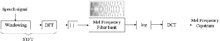
The outline of the computation of Mel frequency cepstral coefficients (MFCC) is shown in Figure 1. In general, the MFCCs are computed as follows. Let $x[n]$ be a speech signal with a sampling frequency of $f_{s}$, and is divided into $P$ frames each of length $N$ samples with an overlap of $N/2$ samples such that $\left\{\vec{x}_{1}[n],\vec{x}_{2}[n]\cdots\vec{x}_{p}[n]\cdots\vec{x}_{P}[n]\right\}$, where $\vec{x}_{p}[n]$ denotes the $p^{th}$ frame of the speech signal $x[n]$ and is $\vec{x}_{p}[n]=\left\{x\left[p*\left(\frac{N}{2}-1\right)+i\right]\right\}_{i=0}^{N-1}$ Now the speech signal $x[n]$ can be represented in matrix notation as ${\cal{X}}\stackrel{{\scriptstyle def}}{{=}}[\vec{x}_{1},\vec{x}_{2},\cdots,\vec{x}_{p},\cdots,\vec{x}_{P}]$. Note that the size of the matrix $\cal{X}$ is $N\times P$. The MFCC features are computed for each frame of the speech sample (namely, for all $\vec{x}_{p}$).

2.1 Windowing, DFT and Magnitude Spectrum

In speech signal processing, in order to compute the MFCCs of the $p^{th}$ frame, $\vec{x}_{p}$ is multiplied with a hamming window $w[n]=0.54-0.46\cos\left(\frac{n\pi}{N}\right)$, followed by the discrete Fourier transform (DFT) as shown in (1).

$$X_{p}(k)=\sum_{n=0}^{N-1}x_{p}[n]w[n]\exp^{-j\frac{2\pi kn}{N}}$$ (1)

for $k=0,1,\cdots,N-1$. If $f_{s}$ is the sampling rate of the speech signal $x[n]$ then $k$ corresponds to the frequency $\color[rgb]{0,0,0}{l_{f}}(k)=kf_{s}/N$. Let $\vec{X}_{p}=[X_{p}(0),X_{p}(1),\cdots,X_{p}(N-1)]^{T}$ represent the DFT of the windowed $p^{th}$ frame of the speech signal $x[n]$, namely $\vec{x}_{p}$. Accordingly, let $X=[\vec{X}_{1},\vec{X}_{2},\cdots\vec{X}_{p},\cdots,\vec{X}_{P}]$ represent the DFT of the matrix $\cal{X}$. Note that the size of $X$ is $N\times P$ and is known as STFT (short time Fourier transform) matrix. The modulus of Fourier transform is extracted and the magnitude spectrum is obtained as $|X|$ which again is a matrix of size $N$ x $P$.

2.2 Mel Frequency Filter Bank

The modulus of Fourier transform is extracted and the magnitude spectrum is obtained as $|X|$ which is a matrix of size $N\times P$. The magnitude spectrum is warped according to the Mel scale in order to adapt the frequency resolution to the properties of the human ear [8]. Note that the Mel ($\color[rgb]{0,0,0}{\phi_{f}}$) and the linear frequency ($\color[rgb]{0,0,0}{l_{f}}$) [9] are related, namely, $\color[rgb]{0,0,0}{\phi_{f}}=2595*log_{10}(1+\frac{\color[rgb]{0,0,0}{l_{f}}}{700})$ where $\color[rgb]{0,0,0}{\phi_{f}}$ is the Mel frequency and $\color[rgb]{0,0,0}{l_{f}}$ is the linear frequency. Then the magnitude spectrum $|X|$ is segmented into a number of critical bands by means of a Mel filter bank which typically consists of a series of overlapping triangular filters defined by their center frequencies $\color[rgb]{0,0,0}{l_{f}}{{}_{c}}(m)$.

The parameters that define a Mel filter bank are (a) number of Mel filters, $F$, (b) minimum frequency, $\color[rgb]{0,0,0}{l_{f}}{{}_{min}}$ and (c) maximum frequency, $\color[rgb]{0,0,0}{l_{f}}{{}_{max}}$. For speech, in general, it is suggested in [10] that $\color[rgb]{0,0,0}{l_{f}}{{}_{min}}>100$ Hz. Furthermore, by setting $\color[rgb]{0,0,0}{l_{f}}{{}_{min}}$ above 50/60Hz, we get rid of the hum resulting from the AC power, if present. [10] also suggests that $\color[rgb]{0,0,0}{l_{f}}{{}_{max}}$ be less than the Nyquist frequency. Furthermore, there is not much information above $6800$ Hz. Then a fixed frequency resolution in the Mel scale is computed using $\delta\color[rgb]{0,0,0}{\phi_{f}}=(\color[rgb]{0,0,0}{\phi_{f}}{{}_{max}}-\color[rgb]{0,0,0}{\phi_{f}}{{}_{min}})/(F+1)$ where $\color[rgb]{0,0,0}{\phi_{f}}{{}_{max}}$ and $\color[rgb]{0,0,0}{\phi_{f}}{{}_{min}}$ are the frequencies on the Mel scale corresponding to the linear frequencies $\color[rgb]{0,0,0}{l_{f}}{{}_{max}}$ and $\color[rgb]{0,0,0}{l_{f}}{{}_{min}}$ respectively. The center frequencies on the Mel scale are given by $\color[rgb]{0,0,0}{\phi_{f}}{{}_{c}(m)}=m.\delta\phi$ where $m=1,2,\cdots,F$. To obtain the center frequencies of the triangular Mel filter bank in Hertz, we use the inverse relationship between $\color[rgb]{0,0,0}{l_{f}}$ and $\color[rgb]{0,0,0}{\phi_{f}}$ given by $\color[rgb]{0,0,0}{l_{f}}{{}_{c}(m)}=700(10^{\color[rgb]{0,0,0}{\phi_{f}}{{}_{c}(m)}/2595}-1)$. The Mel filter bank, $M(m,k)$ [11] is given by

$$\mbox{\scriptsize{$M(m,k)$}}=\left\{\begin{array}[]{ll}\mbox{\scriptsize{0}}&\mbox{\scriptsize{for $\color[rgb]{0,0,0}{l_{f}}(k)<\color[rgb]{0,0,0}{l_{f}}_{c}(m-1)$}}\\ \mbox{\scriptsize{$\frac{\color[rgb]{0,0,0}{l_{f}}(k)-\color[rgb]{0,0,0}{l_{f}}_{c}(m-1)}{\color[rgb]{0,0,0}{l_{f}}_{c}(m)-\color[rgb]{0,0,0}{l_{f}}_{c}(m-1)}$}}&\mbox{\scriptsize{for $\color[rgb]{0,0,0}{l_{f}}_{c}(m-1)\leq\color[rgb]{0,0,0}{l_{f}}(k)<\color[rgb]{0,0,0}{l_{f}}_{c}(m)$}}\\ \mbox{\scriptsize{$\frac{\color[rgb]{0,0,0}{l_{f}}(k)-\color[rgb]{0,0,0}{l_{f}}_{c}(m+1)}{\color[rgb]{0,0,0}{l_{f}}_{c}(m)-\color[rgb]{0,0,0}{l_{f}}_{c}(m+1)}$}}&\mbox{\scriptsize{for $\color[rgb]{0,0,0}{l_{f}}_{c}(m)\leq\color[rgb]{0,0,0}{l_{f}}(k)<\color[rgb]{0,0,0}{l_{f}}_{c}(m+1)$}}\\ \mbox{\scriptsize{0}}&\mbox{\scriptsize{for $\color[rgb]{0,0,0}{l_{f}}(k)\geq\color[rgb]{0,0,0}{l_{f}}_{c}(m+1)$}}\end{array}\right.$$

The Mel filter bank $M(m,k)$ is an $F\times N$ matrix.

2.3 Mel Frequency Cepstrum

The logarithm of the filter bank outputs (Mel spectrum) is given in (2).

$$L_{p}(m,k)=ln\left\{\sum_{k=0}^{N-1}M(m,k)*|X_{p}(k)|\right\}$$ (2)

where $m=1,2,\cdots,F$ and $p=1,2,\cdots,P$. The filter bank output, which is the product of the Mel filter bank, $M$ and the magnitude spectrum, $|X|$ is a $F\times P$ matrix. A discrete cosine transform of $L_{p}(m,k)$ results in the MFCC parameters.

$$\Phi_{p}^{r}\left\{x[n]\right\}=\sum_{m=1}^{F}L_{p}(m,k)\cos\left\{\frac{r(2m-1)\pi}{2F}\right\}$$ (3)

where $r=1,2,\cdots,F$ and $\Phi_{p}^{r}\left\{x[n]\right\}$ represents the $r^{th}$ MFCC of the $p^{th}$ frame of the speech signal $x[n]$. The MFCC of all the $P$ frames of the speech signal are obtained as a matrix $\Phi$

$$\Phi\left\{\cal{X}\right\}=[\Phi_{1},\Phi_{2},\cdots,\Phi_{p},\cdots\Phi_{P}]$$ (4)

Note that the $p^{th}$ column of the matrix $\Phi$, namely $\Phi_{p}$ represents the MFCC of the speech signal, $x[n]$, corresponding to the $p^{th}$ frame, $x_{p}[n]$.

3 MFCC of Resampled Speech

In this section, we show how the resampling of the speech signal in time effects the computation of MFCC parameters. Let $y[s]$ denote the time scaled speech signal given by

$$y[s]=x[\alpha n]=x\downarrow\alpha$$ (5)

where $\alpha$ is the time scale modification (TSM) factor or the scaling factor . Let $y_{p}[s]=x_{p}[\alpha n]=x_{p}\downarrow\alpha$ denote the $p^{th}$ frame of the time scaled speech where $s=0,1,\cdots,S-1$, $S$ being the number of samples in the time scaled speech frame given by $S=\frac{N}{\alpha}$. If $\alpha<1$ the signal is expanded in time while $\alpha>1$ means the signal is compressed in time. Note that if $\alpha=1$ the signal remains unchanged.

DFT of the windowed $y_{p}[n]$ is calculated from the DFT of $x_{p}[n]$. Assuming that $\alpha$ is an integer and using the scaling property of DFT [12], we have,

$$Y_{p}(k^{\prime})=\frac{1}{\alpha}\sum_{l=0}^{\alpha-1}X_{p}(k^{\prime}+lS)$$ (6)

where $k^{\prime}=1,2,\cdots,S$. The MFCC of the time scaled speech are given by

$$\Phi_{p}^{r}\{y[n]\}=\Phi_{p}^{r}\left\{x\downarrow\alpha\right\}=\sum_{m=1}^{F}L_{p}^{\prime}(m,k^{\prime})cos\left\{\frac{r(2m-1)\pi}{2F}\right\}$$ (7)

where $r=1,2,\cdots,F$ and

$$L_{p}^{\prime}(m,k^{\prime})=ln\left\{\sum_{k^{\prime}=0}^{S-1}\tiny{M^{\prime}(m,k^{\prime})}\left|\frac{1}{\alpha}\sum_{l=0}^{\alpha-1}X_{p}(k^{\prime}+lS)\right|\right\}$$ (8)

Note that $L_{p}^{\prime}$ and $M^{\prime}$ are the log Mel spectrum and the Mel filter bank of the resampled speech. We consider various forms of the Mel filter bank, $M^{\prime}(m,k^{\prime})$ which is used in the calculation of MFCC of the resampled speech. The best choice of the Mel filter band is the one which gives the best Pearson correlation between the MFCC of the original speech and the MFCC of the resampled speech.

3.1 Computation of MFCC of Resampled speech

The major step in the computation of MFCC of the resampled speech lies in the construction of the Mel filter bank. The Mel filter bank used to calculate the MFCC of the resampled speech is given by

$$\mbox{\scriptsize{$M^{\prime}(m,k^{\prime})$}}=\left\{\begin{array}[]{ll}\mbox{\scriptsize{0}}&\mbox{\scriptsize{for $\color[rgb]{0,0,0}{l_{f}}(k^{\prime})<\color[rgb]{0,0,0}{l_{f}}^{\prime}_{c}(m-1)$}}\\ \mbox{\scriptsize{$\frac{\color[rgb]{0,0,0}{l_{f}}(k^{\prime})-\color[rgb]{0,0,0}{l_{f}}^{\prime}_{c}(m-1)}{\color[rgb]{0,0,0}{l_{f}}^{\prime}_{c}(m)-\color[rgb]{0,0,0}{l_{f}}^{\prime}_{c}(m-1)}$}}&\mbox{\scriptsize{for $\color[rgb]{0,0,0}{l_{f}}^{\prime}_{c}(m-1)\leq\color[rgb]{0,0,0}{l_{f}}(k^{\prime})<\color[rgb]{0,0,0}{l_{f}}^{\prime}_{c}(m)$}}\\ \mbox{\scriptsize{$\frac{\color[rgb]{0,0,0}{l_{f}}(k^{\prime})-\color[rgb]{0,0,0}{l_{f}}^{\prime}_{c}(m+1)}{\color[rgb]{0,0,0}{l_{f}}^{\prime}_{c}(m)-\color[rgb]{0,0,0}{l_{f}}^{\prime}_{c}(m+1)}$}}&\mbox{\scriptsize{for $\color[rgb]{0,0,0}{l_{f}}^{\prime}_{c}(m)\leq\color[rgb]{0,0,0}{l_{f}}(k^{\prime})<\color[rgb]{0,0,0}{l_{f}}^{\prime}_{c}(m+1)$}}\\ \mbox{\scriptsize{0}}&\mbox{\scriptsize{for $\color[rgb]{0,0,0}{l_{f}}(k^{\prime})\geq\color[rgb]{0,0,0}{l_{f}}^{\prime}_{c}(m+1)$}}\end{array}\right.$$

where $l_{f}(k^{\prime})=\frac{k^{\prime}(f_{s}/2)}{N/2}$.

As mentioned, we consider different forms of Mel filter banks and identify the Mel-filter bank that results in the MFCC value of the resampled speech signal that matches best with the original speech signal MFCC. This is done by computing the Pearson coefficient between the MFCC of the resampled speech and the MFCC of the original speech. The variations in the Mel filter banks is a result of the way in which the center frequencies and the amplitude of the filter coefficients are chosen. In all the cases discussed below, we assume, (a) $\alpha=2$, (b) the number of Mel filters used for the feature extraction of original speech and that of the resampled speech are same and, (c) the window length reduces by half, namely, $N/2$.

3.1.1 Type A and Type B: Downsampling $M(m,k)$

$M^{\prime}(m,k^{\prime})$ is obtained by downsampling $M(m,k)$ by a factor of $\alpha$, namely, $M_{A}^{\prime}(m,k^{\prime})=M(m,\alpha k)$. There are two ways in which the center frequencies of $M^{\prime}_{A}$ are chosen. Type A: same as that of the original center frequencies, namely, $\color[rgb]{0,0,0}{l_{f}}^{\prime}_{c}(m)=\color[rgb]{0,0,0}{l_{f}}_{c}(m)$, and Type B: halving the original center frequencies, namely, $\color[rgb]{0,0,0}{l_{f}}^{\prime}_{c}(m)=\frac{1}{2}\color[rgb]{0,0,0}{l_{f}}_{c}(m)$.

3.1.2 Type C: Constructing new filter bank in the halved band

Here, we halve the frequency band on which the original filter bank ($M$) is constructed and construct a new filter bank following the steps described in Section (2) on the halved band. The minimum and maximum frequencies of the new Mel bank are chosen as $\frac{\color[rgb]{0,0,0}{l_{f}}{{}_{max}}}{2}$ and $\frac{\color[rgb]{0,0,0}{l_{f}}{{}_{min}}}{2}$ respectively.

3.1.3 Type D: Interpolating

Here, alternate center frequencies of the original Mel bank are halved and filters are constructed with the resultant center frequencies. This reduces the bandwidth of the Mel bank and the number of Mel filters by a factor of $2$. The output of these $\frac{F}{2}$ Mel filters are denoted as $[\vec{g_{1}}\vec{g_{2}}\cdots\vec{g_{m}}\cdots\vec{g_{F/2}}]$. and the Mel spectrum is computed as

$$\left[\vec{g_{1}}\;\;\frac{\vec{g_{1}}+\vec{g_{2}}}{2}\;\;\vec{g_{2}}\;\;\frac{\vec{g_{2}}+\vec{g_{3}}}{2}\cdots\vec{g_{m}}\cdots\vec{g_{F/2}}\;\;\frac{\vec{g_{F/2}}+\vec{g_{1}}}{2}\right]$$

DCT of the logarithm of the above vectors gives the MFCC of the down sampled speech.

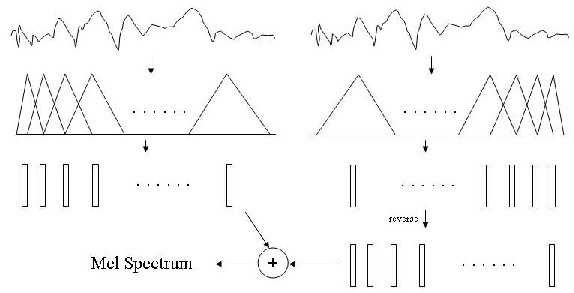
3.1.4 Type E and Type F: Reversing, Adding and Averaging

In this case, the filter bank outputs of the downsampled Mel filter bank, namely, $M_{A}^{\prime}(m,k^{\prime})$ are computed. Then the downsampled Mel filter bank is mirrored/reversed such that the filter with the highest bandwidth comes first and the one with the lowest bandwidth comes last. The spectrum of the downsampled signal is passed through this reversed filter bank and the filter bank outputs are again reversed. These reversed filter bank outputs are added to the former filter bank (downsampled bank) outputs and their average is considered to be the Mel spectrum. DCT of the logarithm of the Mel spectrum gives the MFCC of the down sampled speech. This method also has $2$ cases, namely, Type E: the center frequencies chosen are of type Type A, and, Type F: the center frequencies chosen are of type Type B. This process is depicted in Figure 2.

Figure 2: Type E and F - Reversing, Adding and Averaging.

4 Experimental Results

In all our experiments we considered speech signals sampled at $16$ kHz and represented by $16$ bits. The speech signal is divided into frames of duration $32$ ms (or $N=512$ samples) and $16$ ms overlap ($256$ samples). MFCC parameters are computed for each speech frame using (3). The Mel filter bank used has $F=30$ bands spread from $\color[rgb]{0,0,0}{l_{f}}{{}_{min}}=130$ Hz to a maximum frequency of $\color[rgb]{0,0,0}{l_{f}}{{}_{max}}=6800$ Hz. The MFCC parameters (denoted by $\Phi\{x[n]\}=[\Phi_{1},\Phi_{2},\cdots,\Phi_{m},\cdots\Phi_{F}]$) are computed for the $16$ kHz speech signal $x[n]$, as described in Section 2. Then $x[n]$ is downsampled by a scaling factor of $\alpha=2$ and denoted by $y[s]=x\downarrow 2=x[2n]$. The MFCC parameters of $y[s]$ (denoted by $\Phi\{y[s]\}=[\Phi^{\prime}_{1},\Phi^{\prime}_{2},\cdots,\Phi^{\prime}_{m},\cdots\Phi^{\prime}_{F}]$) are calculated using the six methods discussed in Sections 3.1.1 to 3.1.4. Pearson correlation coefficient (denoted by $r$) is computed between the MFCC parameters of the downsampled speech (using different Mel-filter bank constructs) and the MFCC of the original speech in two different ways.

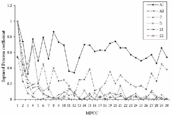
Case I: Pearson correlation coefficient, $r$ between the individual MFCC of the original and the downsampled speech signals, namely, $\Phi_{m}$ and $\Phi^{\prime}_{m}$, $m=1,2,\cdots,F$ is calculated. The variation of the squared Pearson correlation coefficient, $r^{2}$ over individual MFCC ($F=30$) for the $6$ types of Mel filter bank constructs is shown in Figure 3.

Case II: The $F$ MFCC vectors are concatenated to form a single vector and the $r$ between the two vectors corresponding to the original speech and the downsampled speech is computed. The Pearson correlation coefficient, $r$ for the $6$ methods is shown in Table 1 for three different $16$ kHz, $16$ bit speech samples.

Table 1: Pearson correlation ($r$) between the MFCC of original speech and the downsampled speech

Speech A B C D E F Sample 1 0.978 0.945 0.941 0.908 0.844 0.821 Sample 2 0.976 0.947 0.943 0.914 0.889 0.877 Sample 3 0.973 0.947 0.944 0.916 0.895 0.878

As observed from Figure 3 and Table 1, the Type A of constructing Mel filter bank for the down sampled speech gives the best correlation between the MFCC parameters of the original speech and that of the downsampled speech.

Figure 3: Pearson correlation ($r^{2}$) between the MFCC of original speech and downsampled speech (for speech sample 3).

5 Conclusion

The effect of resampling of speech on the MFCC parameters of speech has been presented. We have demonstrated that it is possible to extract MFCC from a downsampled speech by constructing an appropriate Mel filter bank. We presented six methods of computing MFCC of a downsampled speech signal by transforming the Mel filter bands used to compute MFCC parameters. The choice of various transformation of Mel filter bank was based on the relationship between the spectrum of the original and the resampled signal (Equation 6). We have shown that the Pearson correlation coefficient between the MFCC parameters of the original speech and the downsampled speech shows a good fit with a downsampled version of the Mel filter bank (Type A). We believe the results presented in this paper will enable us to experiment and measure the performance of a speech recognition engine (statistical phoneme models derived from original speech) on subsampled speech (time compressed speech).

References

- [1] B. Arons, “Techniques, perception, and applications of time- compressed speech,” Proceedings of 1992 Conference, American Voice I/O Society, pp. 169–177, Sep. 1992.
- [2] D. J. Hejna, “Real-time time-scale modification of speech via the synchronized overlap-add algorithm,” M.I.T. Masters Thesis, Department of Electrical Engineering and Computer Science, February 1990.
- [3] S. B. Davis and P. Mermelstein, “Comparison of parametric representations for monosyllabic word recognition in continuously spoken sentences,” IEEE Trans. Acoust. Speech Signal Processing, vol. 28, no. 4, pp. 357–366, 1980.
- [4] D. A. Reynolds and R. C. Rose, “Robust text-independent speaker identification using gaussian mixture speaker models,” IEEE Transactions on Speech and Audio Processing, vol. 3, No. 1, January 1995.
- [5] M. R. Hasan, M. Jamil, M. G. Rabbani, and M. S. Rahman, “Speaker identification using Mel frequency cepstral coefficients,” 3rd International Conference on Electrical & Computer Engineering ICECE 2004, 28-30 December 2004, Dhaka, Bangladesh.
- [6] H. Seddik, A. Rahmouni, and M. Sayadi, “Text independent speaker recognition using the Mel frequency cepstral coefficients and a neural network classifier,” First International Symposium on Control, Communications and Signal Processing, pp. 631–634, 2004.
- [7] Z. Jun, S. Kwong, W. Gang, and Q. Hong, “Using Mel-frequency cepstral coefficients in missing data technique,” EURASIP Journal on Applied Signal Processing, vol. 2004, no. 3, pp. 340–346, 2004.
- [8] S. Molau, M. Pitz, R. S. Uter, and H. Ney, “Computing Mel-frequency cepstral coefficients on the power spectrum,” Proc. Int. Conf. on Acoustic, Speech and Signal Processing, pp. 73 – 76, 2001.
- [9] T. F. Quatieri, “Discrete-time speech signal processing: Principles and practice,” Pearson Education, vol. II, pp. 686, 713, 1989.
- [10] CMU, “http:// cmusphinx.sourceforge.net/ sphinx4/ javadoc/ edu/ cmu/ sphinx/ frontend/ frequencywarp/ melfrequencyfilterbank.html.”
- [11] S. Sigurdsson, K. B. Petersen, and T. L. Schi ler, “Mel frequency cepstral coefficients: An evaluation of robustness of mp3 encoded music,” Conference Proceedings of the Seventh International Conference on Music Information Retrieval (ISMIR), Vicoria, Canada, 2006.
- [12] Oppenheim and Schafer, “Discrete time signal processing,” Prentice-Hall, 1989.