Power Redistribution for Optimizing Performance
in MPI Clusters

Abstract

Power efficiency has recently become a major concern in the high-performance computing domain. HPC centers are provisioned by a power bound which impacts execution time. Naturally, a tradeoff arises between power efficiency and computational efficiency. This paper tackles the problem of performance optimization for MPI applications, where a power bound is assumed. The paper exposes a subset of HPC applications that leverage cluster parallelism using MPI, where nodes encounter multiple synchronization points and exhibit inter-node dependency. We abstract this structure into a dependency graph, and leverage the asymmetry in execution time of parallel jobs on different nodes by redistributing power gained from idling a blocked node to nodes that are lagging in their jobs. We introduce a solution based on integer linear programming (ILP) for optimal power distribution algorithm that minimizes total execution time, while maintaining an upper power bound. We then present an online heuristic that dynamically redistributes power at run time. The heuristic shows significant reductions in total execution time of a set of parallel benchmarks with speedup up to $2.25$.

I Introduction

Power efficiency in clusters for high-performance computing (HPC) and data centers is a major concern, specially due to the continuously rising computational demand, and the increasing cost and difficulty of provisioning enough power to satisfy such demand. This can be easily observed in the growing size of data centers that serve internet-scale applications. Currently, such data centers consume $1.3\%$ of the global energy supply, at a cost of $\$4.5$ billion. This percentage is expected to rise to $8\%$ by 2020 [7]. In fact, the rise in energy costs has become so prevalent that the cost of electricity for fours years in a data center is approaching the cost of setting up a new data center [2]. This, consequently, results in HPC centers operating at tight power bounds, which in turn affects performance.

Extensive work has studied the trade-off between power efficiency and delay, sacrificing performance in favor of power [6]. However, such sacrifice is intolerable in many applications, such as in HPC and cloud services that need to respect certain responsiveness features. On the contrary, there are approaches that target improving performance, which results in reduced energy consumption. This can be especially beneficial in heterogeneous clusters, which are rapidly becoming a favorable approach as opposed to homogeneous clusters [10]. Improved power efficiency, as well as lower cost and easier and cheaper upgrades are among the advantages of heterogeneous clusters. Reducing energy consumption is indirectly related to our objective of improving performance, yet there is very little work on optimizing power distribution of task dependency systems dynamically.

In this paper, we focus on improving the performance of MPI applications running on an HPC cluster, while satisfying a given power bound. To that end, we present a novel solution to the problem that consists of the following:

• A technique to improve parallelism in MPI applications by stretching the execution of parts of the program that do not require immediate attention. This approach enables the execution of the stretched portion at a lower power level, providing more power to more critical tasks.

• An ILP model that is capable of producing an optimal assignment of power to portions of the program.

• An online power redistribution heuristic that dynamically transfers power from a blocked node to running nodes based on a priority ranking mechanism.

• A novel implementation of an MPI wrapper that is capable of constructing a dependency graph online without the need to modify the code.

Our approach works as follows. We build an abstract model of a program executing in parallel as a set of program instances running on a cluster. To that end, we construct a dependency graph to encode the inter-dependency between blocks of non-synchronized code in the program instances, which we denote as jobs. The dependency graph allows us to identify the periods of time where a node will be blocked waiting on the output of other nodes. We exploit this behavior by stretching jobs so that we minimize the amount of time spent waiting for other nodes. Then, using the power constraints and execution time of jobs, we formulate our performance optimization problem as an integer linear program (ILP). The solution to this problem determines the optimum power-bounds to assign to jobs, such that the total execution time is minimized. We use this solution as a reference of goodness for the problem at hand.

In order to deal with online power redistribution in MPI applications at run time, we introduce an online heuristic. Roughly speaking, the heuristic (see Figure 1) detects when a node is blocked, and distributes its power (which will now drop to idle) over other nodes based on a priority ranking mechanism. We implement this heuristic as a wrapper for MPI, such that using it requires no modification to the program’s source code. The wrapper is able to identify when a node is blocked, and the nodes responsible for blocking it. It communicates this information with a central power distribution controller, which in turn makes a decision on how to distribute the power gained by idling the blocked node.

A significant advantage of the proposed solution is that it is designed to improve performance of HPC applications with minimal requirements. Simply by linking existing code to the proposed MPI wrapper and connecting a low-end embedded board hosting the power distribution controller, a cluster can immediately benefit from dynamic power distribution.

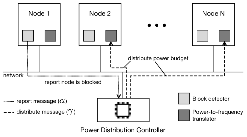
Figure 1: Block diagram of an HPC cluster equipped with power distribution.

To validate our approach, we conduct a set of simulations and actual experiments. First, we simulate a simple MPI program running using equal-share, ILP based, and heuristic based power distribution schemes. The simulation demonstrates the correlation between the variability in execution time and speedup. The improvement in execution time is promising, reaching a speedup of $2.5$ for ILP based distribution and $2.0$ for the heuristic based distribution. To demonstrate the applicability of the approach to homogeneous clusters, we run the simulation where all parallel jobs consume the same amount of time, and all nodes are identical. The speedup in this case is an encouraging $2.0$ for optimal distribution, and $1.64$ for the heuristic based distribution.

We then experiment on a physical environment using two ARM-based boards that vary in CPU, operating system, and manufacturer. We implement our MPI wrapper that detects changes to node state and communicates it with a power distribution controller that executes our online heuristic. Using different benchmarks from the NAS benchmark suite, we demonstrate that our online heuristic can produce speedups up to $2.5$ times, only to be superseded by the optimal which reaches $2.78$ times. We also draw conclusions on the type of MPI program that would benefit most from our online power distribution heuristic.

Organization:  The rest of the paper is organized as follows. Section II introduces a motivating example to demonstrate our approach. Section III outlines a formal definition of the power distribution problem. Section IV presents an algorithm to achieve the optimal solution. Section V details the design of our online heuristic. Section VI presents the simulation results. Section VII presents the MPI specific implementation and the experimental results. Finally, Section VIII discusses related work, while we conclude in Section IX.

II Motivation

This section outlines a motivating example to demonstrate the existence of an opportunity to optimize performance by redistributing power. Listing 1 shows an abridged version of the rank function in the Integer Sort benchmark of the NAS Benchmark Suite [1]. As can be seen in the code, there are $4$ main blocks of computation: The first block spans lines 2 to 7. This is followed by a blocking collective operation at line 8. This sequence continues until the last block spanning lines 17 to 19.

Figure 2 illustrates a possible execution of this function on a $3$-node cluster. In this cluster, a maximum power bound is enforced, and this results in a power cap assigned per node, which limits its CPU frequency. However, it is possible and quite frequent that some nodes finish execution of a block of computation earlier than others, yet a blocking operation forces them to wait. This can be the result of, for instance, using heterogenous nodes, differences in workload, or nodes executing in different execution paths. This is demonstrated in Figure 2 by the dark grey blocks in the figure, which we denote as blackouts. Naturally, execution cannot proceed until all nodes arrive at the barrier. This also applies to node-to-node send and receive operations.

Our research hypothesis is that an intelligent distribution of power can reduce these blackout periods, resulting in reduction of total execution time. This is demonstrated in Figure 3. The thickness of a block indicates how much power it is allowed to consume. Blocks that consume a relatively short time in Figure 2, such as the first block in node 2, operate at a lower power cap in Figure 3 (demonstrated by reduced thickness). An optimum solution is capable of eradicating all blackouts, and minimizing those that are unavoidable (such as a ring send/receive). This results in a reduced total execution time within the cluster power bound.

⬇

1void rank( int iteration ) {

2 for(i=0;i<NUM_BUCKETS+TEST_ARRAY_SIZE;i++) {

3 // Computation

4 }

5 for( i=0; i<TEST_ARRAY_SIZE; i++ ) {

6 // Computation

7 }

8 MPI_Allreduce( $\cdots$ );

9 for( i=0, j=0; i<NUM_BUCKETS; i++ ) {

10 // Computation

11 }

12 MPI_Alltoall( $\cdots$ );

13 for( i=1; i<comm_size; i++ ) {

14 // Computation

15 }

16 MPI_Alltoallv( $\cdots$ );

17 for( i=0; i<TEST_ARRAY_SIZE; i++ ) {

18 // Computation

19 }

20}

Listing 1: Abridged rank method in the NPB IS benchmark

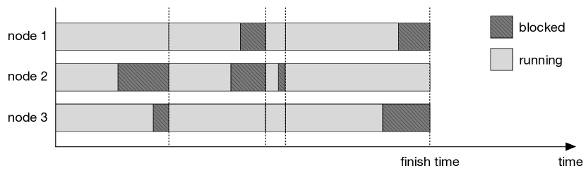
Figure 2: A possible execution of rank on $3$ nodes.

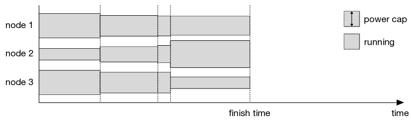
Figure 3: An optimum execution of rank on $3$ nodes using power redistribution.

III Formal Problem Description

This section presents a formal description of the power distribution problem. Consider a set $\mathbb{N}=\{N_{1},N_{2},\dots,N_{n}\}$ of nodes in a parallel computing cluster that is required to satisfy a power bound $\mathbb{P}$. Each node runs a single instance of a parallel program. We model the execution of the program instance on a node as a sequence of jobs:

$$\mathcal{J}_{i}=\left<J_{i,1}J_{i,2}J_{i,j}\cdots\right>$$

where $J_{i,j}$ is the $j^{th}$ job on node $i$. A job represents a block of execution of the program instance on a single node that, once started, can be completed independently and without communication with other nodes. A job is defined as the following tuple:

$$J_{i,j}=\left<\tau(J_{i,j},P),\theta(J_{i,j}),\pi(J_{i,j})\right>$$

where

• $\tau(J_{i,j},P)$ is a function that encodes the execution time of job $j$ on node $i$ operating under power bound $P$, which directly enforces a maximum frequency that the CPU of node $i$ can utilize.

• $\theta(J_{i,j})$ is a function that encodes the dependency of one job on a set of preoccuring jobs with the condition that it does not depend on multiple jobs in any other node. Such behavior can be expressed indirectly by chaining dependency. Naturally, in the serial execution of a program instance on node $i$, every job $j$ is dependent on its predecessor $j-1$. That is, $J_{i,j-1}\in\theta(J_{i,j})$. This implies that the execution of job $j$ cannot begin unless job $j-1$ is completed.

• $\pi(J_{i,j})$ denotes the power bound that node $i$ should honour during execution of job $j$.

Our objective is to determine the mapping $\pi$ of all jobs on all nodes to their power bounds ($\pi(J_{i,j})$) such that:

1. The dependency of jobs $\theta$ is not violated;

2. The cluster power bound $\mathbb{P}$ is not exceeded, and

3. The total execution time is minimized.

III-A Job Dependency Graph

In order to calculate the total execution time, we construct a job dependency graph.

Definition 1 (Job dependency graph)

A job dependency graph $D$ is a directed acyclic graph, where vertices represent jobs $J_{i,j}$ and directed edges represent the dependency relation as described by $\theta$, such that if $(J_{i,j},J_{i^{\prime},j^{\prime}})$ is a directed edge of $D$, then $J_{i,j}\in\theta(J(i^{\prime},j^{\prime}))$.∎

The job dependency graph is acyclic since a cycle will indicate circular dependency of jobs, which is impossible to occur since a job cannot be dependent on itself, directly or indirectly.

III-B Total execution time

To discuss the total execution time, we first define the following:

• Initial Job ($J^{I}$). An initial job is a job that does not depend on any other job to begin execution, that is $\theta(J^{I})=\{\}$. Normally an initial job is the first block of execution of a program instance on some node, up until the point of communication which is dependent on one or more other nodes. An initial job in a job dependency graph has no incoming edges.

• Final Job ($J^{F}$). A final job is a job on which no other job depends. This is normally the final job to be executed by some node. A final job in a job dependency graph has no outgoing edges.

Given the notions of an initial job and a final job, we can now define an execution path.

Definition 2 (Execution path)

An execution path $\rho$ is a path from an initial job to a final job ($J^{I}\rightsquigarrow J^{F}$) in a job dependency graph. Clearly, such a path is a sequence of jobs:

$$\rho=\left<J^{I}_{i,j},J_{i^{\prime},j^{\prime}},\cdots,,J^{F}_{i^{\prime\prime},j^{\prime\prime}}\right>$$

such that every job in the sequence is dependent on its predecessor, that is $J_{i,j}\in\theta(J(i^{\prime},j^{\prime}))$. We use the notation $\rho(l)$ to indicate the $l^{th}$ job in path $\rho$. ∎

The next step in preparing to calculate the total execution time is defining the scaling factor function $\mathcal{S}$. Let $\varrho=\{\rho_{1},\rho_{2},\rho_{k},\cdots\}$ be the set of all execution paths in a job dependency graph $D$. The execution time $\epsilon$ of a path $\rho$ is calculated as follows:

$$\epsilon(\rho)=\sum_{l=0}^{|\rho|}{\tau(\rho(l),\pi(\rho(l)))}$$ (1)

Thus, the execution time of a path is the sum of execution times of all the jobs in the path, given their respective power bounds. We can now define the total execution time.

Definition 3 (Total execution time of a parallel program)

Let a job dependency graph $D$ contain a set of execution paths $\varrho_{D}=\{\rho_{1},\rho_{2},\rho_{k},\cdots\}$, and let the set $E_{D}=\{\epsilon(\rho_{1}),\epsilon(\rho_{2}),\epsilon(\rho_{k}),\cdots\}$ indicate the execution time of each path as mentioned above. We define the total execution time as $\mathbb{E}_{D}=\underset{k}{\text{max}}\left\{\epsilon(\rho_{k})\right\}$ ∎

Thus, the total execution time of a parallel program is the execution time of the longest execution path in the program’s job dependency graph.

III-C Example of a Job Dependency Graph

To demonstrate how a job dependency graph is constructed and how it is used to determine the total execution time of a parallel program, in this section, we introduce a simple MPI program as our running example throughout the paper. The program performs a set of commonplace MPI operations. The code in Listing 2 demonstrates an MPI program that goes through 3 steps:

1. Broadcasts a message from the root node.

2. Sends a message between nodes in a ring.

3. Performs a reduction on a variable.

Assume this program runs in a cluster of $3$ nodes. Based on the steps mentioned earlier, nodes will execute the following jobs:

• $J_{\_,1}$: represents lines 2-11. This is applicable to all nodes.

• $J_{0,2}$ represents lines 13-21. However, $J_{1,2}$ and $J_{2,2}$ represent lines 13-25.

• $J_{0,3}$ represents line 22, while the other two nodes represent line 27.

• $J_{\_,4}$ represents lines 30-31.

• $J_{\_,5}$ represents line 32.

⬇

1void main(int argc, char *argv[]) {

2 int msg1, msg2, msg3;

3 int rank, size, next, prev;

4 MPI_Init(&argc, &argv);

5 MPI_Comm_rank(MPI_COMM_WORLD, &rank);

6 MPI_Comm_size(MPI_COMM_WORLD, &size);

7

8 if (rank == 0)

9 msg1 = 10;

10

11 MPI_BCast(&msg1,1,MPI_INT,0,MPI_COMM_WORLD);

12

13 next = (rank + 1) % size;

14 prev = (rank + size - 1) % size;

15

16 if (rank == 0)

17 msg2 = size;

18

19 if (rank == 0) {

20 msg2--;

21 MPI_Send(&msg2, 1, MPI_INT, next, rank, MPI_COMM_WORLD);

22 MPI_Recv(&msg2, 1, MPI_INT, prev, prev, MPI_COMM_WORLD);

23 }

24 else {

25 MPI_Recv(&msg2, 1, MPI_INT, prev, prev, MPI_COMM_WORLD);

26 msg2--;

27 MPI_Send(&msg2, 1, MPI_INT, next, rank, MPI_COMM_WORLD);

28 }

29

30 msg2 = rank;

31 MPI_Reduce(&msg2, &msg3, 1, MPI_INT, MPI_MIN, 0, MPI_COMM_WORLD);

32 MPI_Finalize();

33}

Listing 2: A simple MPI program.

In total, there are $15$ jobs in the system. Figure 4 presents the dependency graph of the program with some hypothetical job execution times. These execution times are a result of applying the same power bound $\mathcal{P}$ on every node in the cluster, which we denote as the nominal power bound. The nominal power bound $\mathcal{P}$ is equal to $\mathbb{P}/N$, simply distributing the cluster power bound equally among all nodes in the system. Every block in the figure represents a job, which can be identified by its column, indicating to what node the job belongs to, and its row, indicating the index of that job in the sequence of node jobs. The nominal execution time of each job (that is $\tau(J_{i,j},\mathcal{P})$) is indicated by the number inside the block. The arrows represent dependency among nodes. As can be seen in the figure, the longest execution path starts with $J_{2,1}$ and proceeds along the dashed lines. Hence, the total execution time is $19$ time units.

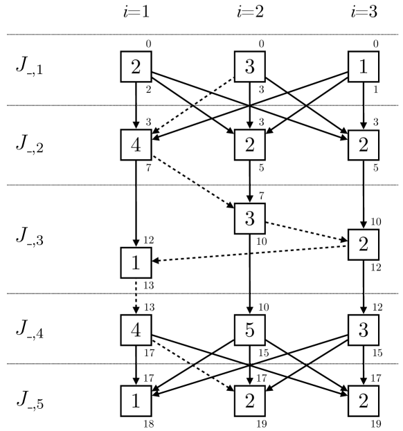
Figure 4: Dependency graph of the program in Listing 2.

Now, let us validate that the longest execution path is indeed indicative of the total execution time:

• Execution starts at job $0$ in all nodes, which is a block of code that ends with a call to MPI_BCast. A broadcast operation is an implicit barrier, and, hence, no node can proceed unless all $J_{\_,1}$ jobs are completed. This is visualized by connecting every $J_{\_,2}$ job with every $J_{\_,1}$ job.

• Since $J_{2,1}$ takes the longest time, all $J_{\_,2}$ start after $3$ time units. This is indicated by the superscript of these blocks in the figure.

• $J_{2,2}$, which ends with a call to MPI_Recv, will block execution until node $1$ completes $J_{1,2}$ which ends with a call to MPI_Send. Thus, $J_{2,3}$ is dependent on both its predecessor $J_{2,2}$ and $J_{1,2}$ which will send a message. The consequence of this dependency is that $J_{2,3}$ executes at $7$ time units, which is the maximum of the completion times of $J_{2,2}$ and $J_{1,2}$, as indicated by the subscript of the respective blocks.

• If we follow this process we can determine the completion time of all nodes, indicated by the subscript of the final jobs $J^{F}_{\_,5}$, after which the program terminates. The last jobs to complete are $J_{2,5}$ and $J_{3,5}$, which finish after $19$ time units.

As shown in Figure 4, the execution time of the longest path is the time at which all nodes in the cluster finish execution.

IV Optimal Solution

This section presents a method based on integer linear programming (ILP) to obtain the optimal solution for the power distribution problem. We, in particular, develop this method, so we have a reference of goodness for our online algorithm in Section V.

In order to limit the number of variables in the ILP instance, we design an algorithm that establishes potential interleavings among jobs executing in different nodes. This algorithm is similar to real-time scheduling algorithms for task dependency on multiprocessors, with the added dimensions of job power bounds and variable execution times. The following subsection introduces the Job Concurrency Optimization algorithm.

IV-A Job Concurrency Optimization Algorithm

The job concurrency optimization algorithm determines which jobs can execute concurrently without violating the dependency structure encoded in the job dependency graph. Since our objective is to reduce the length of blackouts, we can make an abstraction and avoid exploration of all possible interleavings in a parallel program. First, we begin by introducing the following definitions.

Definition 4 (Job Max-Depth)

The max-depth $\delta$ of a job $J$ in a job dependency graph $D$ is the length of the longest path that starts from the initial job and ends with job $J$. That is

$$\delta(J)=\max\left\{l\mid\rho(l)=J\;\wedge\;\rho\in\varrho_{D}\right\}$$

∎

Definition 5 (Job Depth Range)

The depth range $\Delta$ of a job $J$ in a job dependency graph $D$ is an integer interval defined as follows:

$$\Delta(J)=[\delta(J),\beta(J)-1]$$

where $\delta(J)$ is the max-depth of job $J$ and the start of the interval, and $\beta(J)$ is the minimum max-depth of all $J$’s children, that is the set of jobs that are dependent on $J$:

$$\beta(J)={\text{min}}\left\{\delta(J^{\prime})\mid J\in\theta(J^{\prime})\right\}$$

where $J^{\prime}$ is a job in the job dependency graph.∎

Let us clarify the use of these definitions by referring to our earlier example in Listing 2, and the respective job dependency graph in Figure 4. Table I shows the max-depths of all the jobs in the graph. Note that the max-depth is affected by the ring of sends/receives in job $3$ across all $3$ nodes. Figure 5 visualizes how max-depths map to concurrency in execution. The dark grey blocks represent blackout periods, which should be optimally eradicated to reduce total execution time.

TABLE I: Max-depths of jobs in Figure 4.

	Node 1	Node 2	Node 3
Job 1	0	0	0
Job 2	1	1	1
Job 3	4	2	3
Job 4	5	3	4
Job 5	6	6	6

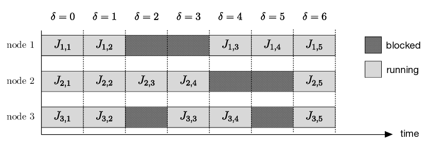
Figure 5: Job concurrency as indicated by job max-depths.

Table II shows the depth ranges of all jobs in the graph. The depth ranges allow us to revisit the job concurrency in Figure 5 to produce an assignment that exhibits less blackouts. Figure 6 demonstrates applying depth ranges to determine optimum job concurrency. Observe job $J_{3,2}$ in the figure, which represents the code executed after the MPI_BCast and before the MPI_Recv called by the third node. The next block of code to be executed by node $3$ requires that node $2$ sends a message ($J_{2,3}$). This implies that the execution of $J_{3,2}$ can be stretched beyond its max-depth level until node $2$ sends a message. Stretching a job in this manner implies allowing it to operate at a lower power level, thus enabling a higher power cap for other nodes in the cluster.

TABLE II: Depth ranges of jobs in Figure 4.

	Node 1	Node 2	Node 3
Job 1	[0,0]	[0,0]	[0,0]
Job 2	[1,1]	[1,1]	[1,2]
Job 3	[4,4]	[2,2]	[3,3]
Job 4	[5,5]	[3,5]	[4,5]
Job 5	[6,6]	[6,6]	[6,6]

Figure 6: Job concurrency after applying depth ranges.

Thus, Figure 6 shows that utilizing depth ranges helps remove blackout periods in execution, except for unavoidable blackouts such as a message ring as shown in our example.

The algorithm is simple to implement, since calculating the max-depths of jobs in the dependency graph is a straight-forward node traversal, and the complexity is $O(E)$, where $E$ is the number of edges in the graph. Finding max-depth in the case of the job dependency graph is thus linear in the size of the graph. Likewise, computing depth ranges requires iterating over the outgoing edges of every job in the graph, resulting in similar complexity.

IV-B ILP Instance

This section introduces the ILP instance used to find the optimum power bound assignment $\pi$, which assigns a power bound to every job in the dependency graph. Refer to Figure 6, which shows how depth ranges reduce blackouts. Note that the figure does not represent the actual execution times of all jobs. For instance, the execution time of jobs $J_{\_,1}$ in Figure 4 are $2$, $3$, and $1$, respectively. This implies a blackout will exist at node $1$ between $2$ and $3$ time units, and at node $3$ between $1$ and $3$ time units. Figure 7 illustrates how such blackouts would occur.

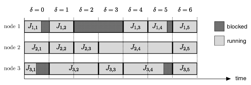
Figure 7: Blackouts in execution due to difference in execution time.

Solving the ILP instance produces a set of power-bound assignments to jobs that minimizes these blackout periods. The ILP instance is detailed as follows.

Variables. The ILP instance abstracts the range of power bounds that can be applied to a certain node into a finite set of power bounds that map to operating frequencies of the node’s CPU. This is a reasonable abstraction since any CPU supports a finite set of operating frequencies, and we can hypothetically determine the power ceiling of the node when operating at every respective frequency. Hence, we introduce the following variables:

• (Job-to-power-bound-assignment $x_{j,b}$) This is a binary variable that indicates whether job $j$ is assigned to power bound $b$. In a dependency graph consisting of $10$ jobs, where each job can operate at $5$ different power bounds, the ILP model will contain $50$ job-to-power-bound-assignment variables.

• (Maximum execution time $t$) This variable represents the maximum time it takes any node in the system to finish execution.

Constraints. The model employs $3$ types of constraints.

• (Unique power bound assignment) These constraints ensure that no job is assigned to two different power bounds. There is one such constraint per job in the graph.

  $$\forall j:\sum_{b}{x_{j,b}}=1$$

• (Cluster power bound enforcement) These constraints enforce the power bound $\mathbb{P}$ on the entire cluster. Generating these constraints relies on the output of the job concurrency optimization algorithm (refer to Figure 6). Every depth level column indicates which jobs will execute concurrently. For instance, job $J_{3,2}$ is concurrent with $\{J_{2,2},J_{1,2}\}$ at depth level $\delta=1$. It is also concurrent with $J_{2,3}$ at depth level $\delta=2$. Hence, there is one power bound enforcement constraint per depth level in the graph:

  $$\forall\delta:\sum_{\delta_{j}}{x_{j,b}\times b}\leq\mathbb{P}$$

  where $\delta_{j}$ is a set that contains any job for which $\delta$ is within its depth range:

  $$\delta_{j}=\{J\mid\delta\in\Delta(J)\}$$

• (Maximum execution time) These constraints ensure that no node executes beyond the maximum execution time variable $t$, which is the variable to be minimized.

  $$\forall i:\sum_{j\in\mathcal{J}_{i}}{\sum_{b}{x_{j,b}\times\tau(j,b)}}\leq t$$

  where $i$ indicates the node, $\mathcal{J}_{i}$ is the sequence of jobs in that node, $j$ is a job in that sequence, and $\tau(j,b)$ is the execution time of job $j$ under power bound $b$.

The total number of constraints in the model is the result of the following formula:

$$\sum_{i}{|\mathcal{J}_{i}|}+\underset{J}{\text{max}}\{\delta(J)\}+n$$

where $n$ is the number of nodes.

Optimization objective. Finally, the objective of the model is to minimize the maximum execution time:

$$\min\;t$$ (2)

V Online Heuristic for Power Redistribution

This section introduces the design of an online heuristic that dynamically distributes power. We approach the design of the heuristic with the following set of objectives:

• The optimum solution introduced in the previous section requires the knowledge of the execution time of every job at every CPU frequency. This is not realistically available for a running application, and, hence, obtaining an optimum online solution is not possible. Thus, our objective is to build an algorithm that receives realistic input and can make online decisions.

• Making power distribution decisions must incur minimal overhead; i.e., in a thrashing-free manner.

• Design the algorithm to be lightweight, executable on non-sophisticated power-efficient hardware.

The heuristic targets HPC clusters composed of heterogenous nodes. Figure 1 illustrates the structure of such a cluster, and introduces the following components:

• Block detector. The block detector is responsible for detecting when a node becomes blocked, awaiting some input from one or more other nodes. It is also responsible for detecting when the node becomes active again. it reports these changes in state to the power distribution controller. The block detector is further explained in Subsection V-A.

• Power distribution controller. The power distribution controller receives messages whenever a node is blocked or unblocked. Since the blocked node will transition to idle, the total power consumption of the cluster will drop. This will provide a power budget that can be distributed to other nodes. The power distribution controller makes a decision on how to distribute the power budget on running nodes. The decision procedure is the core of our online heuristic, which is explained in detail in Subsection V-B.

• Power-to-frequency translator. This component receives the distribute message and translates the power bound dictated by the power distribution controller to a CPU frequency. It selects the maximum CPU frequency that can satisfy the power bound in the message and forces the node to operate at that frequency.

V-A Block Detector

As shown in Figure 1, the block detector sends a report message to the power distribution controller whenever a change in the node state is detected. A report message is a tuple defined as follows:

$$\alpha=\left<s,i,B,p_{g}\right>$$

where

• $s$ is the state of the node, whether Blocked or Running.

• $i$ is the index of the node from which the report message originated.

• $B$ is a set of node indices that are causing node $i$ to be blocked. If $s=\textsf{\small Running}$, $B$ becomes an empty set.

• $p_{g}$ is the power gained by blocking node $i$, which is calculated as follows:

  $$p_{g}=p_{f_{c}}-p_{s}$$

  where $f_{c}$ is the CPU frequency before the block is encountered, $p_{f_{c}}$ is the power consumed by running the CPU at frequency $f_{c}$, and $p_{s}$ is the idle power.

To compute $p_{g}$, we require that each node hosts a lookup table mapping CPU frequency to power. This is obtained by executing a simple benchmark that loads the CPU $100\%$ at each frequency, and records the power consumption. However, if a node hosts a multicore CPU and is executing multiple jobs concurrently, one per core, the power gain becomes the current power minus the power consumed when one less core is active. Hence, we require that the lookup table includes the power consumption of the node at each available frequency and at every possible number of active cores. For instance, a quad-core CPU that supports $10$ different frequencies will result in a lookup table of $40$ entries. An entry will be identified by (1) the number of active cores in parallel (e.g., $1-4$ for quad-core CPUs), and (2) the CPU frequency.

To formally define this, let $p_{m,f}$ be the power consumption of the node when $m$ cores are active and the CPU frequency is $f$. Let $m_{c}$ and $f_{c}$ be the number of active cores and the CPU frequency before the block is encountered on a job executing in one core. In that case, $p_{g}$ is calculated as follows:

$$p_{g}=p_{(m_{c}-1,f_{c})}-p_{s}$$ (3)

V-B Power Distribution Controller – Online Heuristic Design

Algorithm 1 details the logic behind the power distribution heuristic. The heuristic is initialized with a cluster power bound $\mathbb{P}$ watts and an empty (online) dependency graph $G=(V,E)$. The following steps detail the operation of the heuristic:

1. The function ProcessMessage is invoked whenever the power distribution manager receives a report message $\alpha$ from any node in the cluster (line 4).

2. Lines 5-12 in function ProcessMessage update the online dependency graph using the received message. ProcessMessage creates a vertex for the node if it does not already exit, and connects the vertex to other vertices representing nodes that are blocking the sender node.

3. Lines 13-18 calculate the available power budget by adding the power gain $p_{g}$ of all blocked nodes in the graph.

4. The function then calls RankGraph which calculates the priority of a node based on the number of other nodes that it is blocking. A node of rank $0$ has no incoming edges, and hence is not blocking any node. A node of rank $1$ blocks one other node, and so on.

5. Finally, function DistributePower is responsible for distributing the power budget over running nodes. If a node is blocking two other nodes, it will receive twice the amount of power received by a node that is blocking only one other node. This strategy allows the system to gradually increase the power bound of the older blocking nodes, since every time any node is blocked, the older blocking node receives a portion of the power gain.

1:INPUT: Cluster power bound $\mathbb{P}$, number of nodes $n$

2:declare $G=(V,E)$, initially $V=E=\{\}$ $\triangleright$ Online Dependency Graph

3:declare $p_{o}=\mathbb{P}/n$

4:function ProcessMessage($\alpha$)

5:    if $\alpha.i\not\in V$ then

6:        $v\leftarrow$ AddVertex($V$, $\alpha.i$)

7:    else

8:        $v\leftarrow V[\alpha.i]$

9:    end if

10:    $v.s\leftarrow\alpha.s$

11:    $v.p_{g}\leftarrow\alpha.p_{g}$

12:    UpdateEdges($G$, $v$, $\alpha.B$) $\triangleright$ Update connections of $v$ using $\alpha$

13:    declare $\varepsilon=0$ $\triangleright$ Power budget

14:    for $u\in V$ do

15:        if $u.s=\text{Blocked}$ then

16:           $\varepsilon\leftarrow\varepsilon+u.p_{g}$

17:        end if

18:    end for

19:    $t\leftarrow$ RankGraph

20:    DistributePower($\varepsilon$, $t$)

21:end function

22:function UpdateEdges($G$, $v$, $B$)

23:    ClearOutgoingEdges($v$)

24:    for $u\in B$ do

25:        AddEdge($E$, $v$, $u$)

26:    end for

27:end function

28:function RankGraph

29:    $t\leftarrow 0$

30:    for $u\in V$ do

31:        if $u.s=\text{Running}$ then

32:           $u.r\leftarrow|\{e=(a,b)\in E\mid e.b=u\}|$

33:           $t\leftarrow t+u.r$ $\triangleright$ Sum of all ranks

34:        end if

35:    end for

36:    return $t$

37:end function

38:function DistributePower($\varepsilon$, $t$)

39:    for $u\in V$ do

40:        if $u.s=\text{Running}$ then

41:           $p_{b}^{\prime}=p_{o}+\varepsilon\times u.r/t$

42:           if $u.p_{b}\neq p_{b}^{\prime}$ then

43:               $u.p_{b}=p_{b}^{\prime}$

44:               $\gamma\leftarrow(u.i,u.p_{b})$

45:               SendPowerBound($\gamma$)

46:           end if

47:        end if

48:    end for

49:end function

Algorithm 1 Power distribution online heuristic.

VI Simulation results

To validate the intuition behind our model, the ILP solution, and the online heuristic, we implement a simulator to calculate the total execution time of an MPI program. The simulator is initialized with the following:

• a text file detailing the job dependency graph,

• a cluster power bound, and

• the type of simulation: Equal-share, ILP, or Heuristic.

The Equal-share simulation assigns equal power bounds to all nodes in the cluster. The ILP simulation first solves the power assignment problem for an optimal (or nearly optimal due abstractions) solution, and then simulates execution using the resulting job-to-power-assignments. The Heuristic simulation applies the online power distribution algorithm.

Figure 8 shows the results of simulating the dependency graph in Figure 4. The power-to-frequency lookup values, as well as the execution time of jobs at different CPU frequencies are measured on an Arndale Exynos 5410 ARM board. The results indicate that the ILP-based solution excels at the lower power bounds, producing a $2.5$ speedup versus equal-share. The heuristic also produces a significant speedup of $2$ at lower power bounds. The improvement for both ILP-based solution and the heuristic decreases until it matches the execution time of equal-share as the power bound is relaxed. This is expected since at a relaxed power bound the nodes are already operating at their maximum frequencies.

These results are based on the assigned execution times in the job dependency graph in Figure 4, which are completely synthetic. To add some notion of ground truth to the simulations, we rerun the simulation given that the execution times of all jobs is the same. Hence, no bias exists that would favor a power distribution alternative to equal-share. In such a case, the ILP-based solution still outperforms equal-share at lower power bounds, producing a speedup of $2$, while the heuristic speedup is $1.64$. The improvement comes from the fact that the ring communication pattern forces blocking in the equal-share distribution, even when the execution times of jobs is the same. This is improved significantly by applying the stretching of jobs across multiple depth levels, and distributing power optimally on running nodes.

In light of these results, we construct a set of experiments based on the same dependency graph, yet varying in execution times. We quantify the variation in execution times using the standard deviation of execution times of individual jobs. Hence, the experiments present synthesized execution times to target specific standard deviations. The standard deviation starts at $0$ and increases till $6$, given a mean of $10$ time units. Figure 9 illustrates the speedup gained by running the heuristic and the ILP solution, given the minimum possible cluster power bound. The figure shows a trend of increasing speedup as the variation increases, which confirms our intuition that our algorithms excel when execution times exhibit more variability. Yet, at high variability, speedup becomes unstable since it is heavily dependent on the specific execution times assigned to jobs.

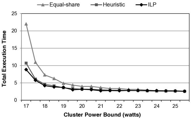
Figure 8: Simulation results of the dependency graph in Figure 4.

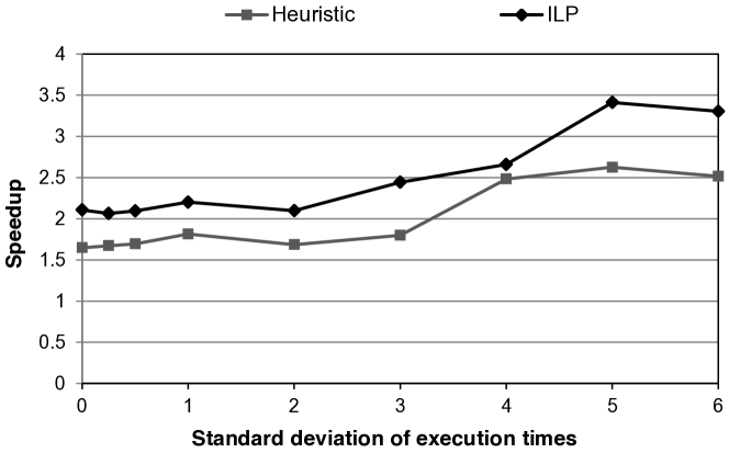
Figure 9: Simulation results using different standard deviations of execution times.

VII Implementation and Experimental Results

VII-A Implementation

Although the model proposed in the paper can generally map to clusters that exhibit task dependency, we focus our implementation on MPI clusters. To that end, we implement an MPI wrapper with underlying logic to perform the functionality of the Block Detector (see section V-A). The power distribution controller is implemented as a standalone lightweight UDP server that receives report messages and responds with distribute messages.

VII-A1 MPI wrapper

The MPI wrapper is designed to intercept MPI calls and deduce whether the node will be blocked or unblocked. Currently the wrapper supports MPI_Send, MPI_Recv, MPI_BCast, MPI_Wait, MPI_Scatter, MPI_Reduce, and MPI_AlltoAll.

The wrapper uses the parameters of the MPI call to deduce the nodes that are blocking the current node, and then creates a report message and transmits it to the power distribution controller. Listing 3 shows an abridged version of the MPI_BCast wrapper. The function power_gain() in line 6 calculates the power gain according to Equation 3. Function all_other_nodes() in line 7 returns the identifiers of all nodes in the cluster with the exclusion of the current node. Since the operation is a broadcast, the current node will in fact not proceed with execution until all other nodes in the cluster have reached the same MPI_BCast call.

⬇

1int pMPI_Bcast(void *buffer, int count, MPI_Datatype type, int root, MPI_Comm comm)

2{

3 report_message msg;

4 msg.node_id = my_rank;

5 msg.state = Blocked;

6 msg.power_gain = power_gain();

7 msg.blocking_nodes = all_other_nodes(my_rank);

8 send(msg);

9

10 int ret = MPI_BCast(buffer,count,type,root,comm);

11

12 msg.state = Running;

13 msg.blocking_nodes = 0;

14 send(msg);

15 return ret;

16}

Listing 3: MPI_BCast wrapper.

VII-A2 Report Manager

A report manager is responsible for sending report messages to the power distribution controller. The report manager initially buffers any message until a predefined timeout has passed. Once the timeout expires, the report manager observes the messages queued up in its internal buffer. If a message is followed by another message that cancels it, the report manager skips both messages. For instance, the send call in line 8 is queued first, and then the send call in line 14. If the timeout expires and the socket manager finds both sends in the buffer, it discards both messages. This behavior helps avoid thrashing the CPU frequency and the power distribution controller with frequent and opposing changes. The timeout period is determined using the breakeven solution to the popular ski-rental problem. In this case, the breakeven point is equivalent to the round-trip-time of a report message to be sent to the power distribution controller, and the distribute message to be sent to the affected nodes. If the MPI_BCast call ends before the round-trip-time, the report manager avoids thrashing by discarding the message, otherwise it sends the report message. The worst case of the breakeven algorithm is that the MPI_BCast call ends immediately at the round-trip-time, in which case sending the report message will not result in any improvement in the performance.

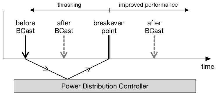
Figure 10: The breakeven point at which the report manager checks the buffer.

The wrapper is missing implementations for MPI_IRecv and other asynchronous functions. Also, it lacks support for multiple communicators, which would require a hierarchical approach to power distribution.

VII-B Experimental setup

To validate the heuristic in practice, we run $3$ MPI benchmarks on $2$ ARM based boards: (1) Arndale Exynos 5410, hosting a dual-core A15 CPU, and (2) odroid XU-2, hosting a quad-core A15 CPU. ARM has recently gained traction in the HPC domain as a power efficient contender to intel [9, 3]. The Arndale board runs linaro ubuntu trusty ($14.04$), while the odroid runs linaro ubuntu raring ($13.04$). This selection of varying manufacturer, CPU capabilities, and OS and kernel versions mimics what would be available at a larger scale in heterogenous clusters. Both boards use OpenMPI 1.8.2, and are connected to an Extech 380803 Power Analyzer that measures their collective power consumption.

We run $3$ benchmarks in the NAS Parallel Benchmark suite (NPB). The benchmarks are as follows:

• IS. An integer sort benchmark that is memory intensive.

• EP. Embarrassingly parallel benchmark that is CPU intensive.

• CG. The conjugate gradient benchmark that is communication intensive.

For each benchmark, we run three problem size classes: A, B and C. The cluster power bound $\mathbb{P}$ for all experiments is $13$ watts, which is a moderately aggressive power bound given the operating power levels of both boards. We repeat each experiment 3 times to ensure the results are not biased by noise.

VII-C Experimental Results

Figures 11, 12, and 13 show the results of executing the IS, EP and CG benchmarks respectively. In the case of IS, the heuristic speed up improves at large problem sizes. This is attributed to the ability of the heuristic to improve performance when the difference in execution time between nodes increases. The power consumption of all three power distribution methods is roughly similar, however, the heuristic power consumption is almost always higher than equal-share or ILP. This observation applies to all three benchmarks, and is attributed to the time discrepancy between a node running after being blocked, and the power distribution controller informing other nodes to lower their power levels to accommodate for the surge that occurs due to the now active node.

The speedup produced by the heuristic is significantly increased in EP, which is expected since the benchmark is heavily CPU bound. At class C, speedup reachers $2.25$, and approaches ILP speedup of $2.78$. This result indicates that the heuristic is better suited for CPU bound MPI programs.

Finally, the heuristic shows inability to improve the CG benchmark. Being communication intensive, the heuristic suffers from two weaknesses: (1) it has very limited time to distribute power more efficiently, rendering it ineffective, and (2) it suffers from some unavoidable thrashing due to the frequency of communication in the program. The interesting point to make here is that the heuristic has minimal negative effect on performance. Out of the $9$ trials associated with CG, one trial produced a speed-down of $0.98$. This seemingly scalable stability is attributed to the efficiency of power distribution. Since changing CPU frequency induces minimum overhead versus for instance efficiently distributing workload.

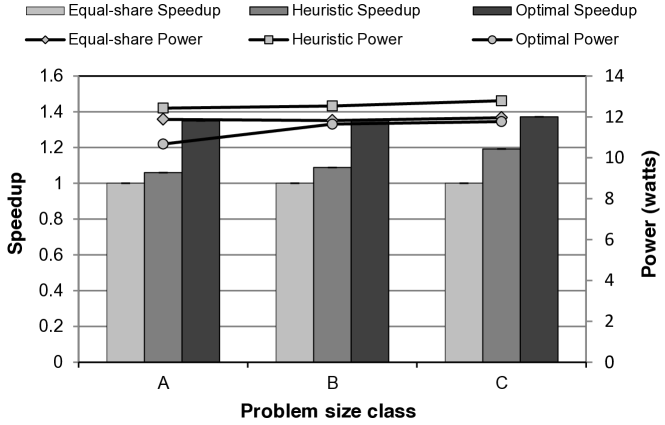
Figure 11: Speedup and average power consumption of the IS benchmark.

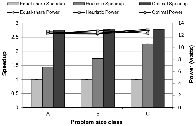
Figure 12: Speedup and average power consumption of the EP benchmark.

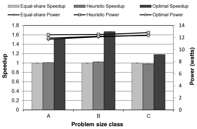
Figure 13: Speedup and average power consumption of the CG benchmark.

VIII Related Work

Recent approaches to improve performance of heterogenous clusters rely on applying load-balancing techniques, where the workload is altered to match the computational capabilities of specific nodes [5]. Our approach does not require redesigning parallel algorithms to support heterogeneous clusters, since the heuristic adapts to variability in execution time whether caused by an unbalanced workload or non-equivalent computational capabilities.

The work in [8, 4] provides a strong foundation on which we base our work. Our approach build on top of this work to introduce a dependency model that can be exploited to improve performance within a power bound.

The work in [11] tackles the problem of scheduling dependent jobs on heterogeneous multiprocessors. Our approach attempts to tackle the problem from a power perspective, in the sense that we transfer power dynamically from one node to another upon detecting dependency. This approach helps produce significantly higher speedups than monitoring each node independently. Our implementation of the heuristic requires no knowledge of the deadlines or execution times of workloads, and infers dependency online using parameters of MPI calls.

IX Conclusion

In this paper, we tackled the problem of optimizing the performance of MPI programs on HPC clusters subject to a power bound. There is little work on this problem in the literature, but we argue that given energy constraints of HPC clusters and data centers and the increasing demand for computing power, we are in pressing need to address the problem. We introduced a formulation of the power distribution problem, and presented an ILP-based solution to obtain the optimal job-to-power-bound assignment. We then introduced an online heuristic that detects when a node is blocked and, subsequently, redistributes its power to other nodes based on a ranking algorithm. We validated the approach using simulation and actual experiments. Our online heuristic produces a speedup of up to a factor of $2.25$, specially in CPU bound programs, while it is ineffective in communication intensive applications.

For future work, we planning on running larger experiments on real-sized HPC clusters. An interesting research problem is to leverage more information about the program using static analysis in an effort to build a smarter heuristic. Also, integrating learning mechanisms in the heuristic will allow it to make more efficient power distribution decisions.

References

- [1] David H Bailey, Leonardo Dagum, Eric Barszcz, and Horst D Simon. Nas parallel benchmark results. In Proceedings of the 1992 ACM/IEEE conference on Supercomputing, pages 386–393. IEEE Computer Society Press, 1992.
- [2] Luiz André Barroso. The price of performance. Queue, 3(7):48–53, 2005.
- [3] Jeffrey Burt. Intel, ARM take competition into HPC arena. http://www.eweek.com/servers/intel-arm-take-competition-into-hpc-arena.html, 2014. [Online; accessed 18-October-2014].
- [4] Anshul Gandhi, Mor Harchol-Balter, Rajarshi Das, and Charles Lefurgy. Optimal power allocation in server farms. In ACM SIGMETRICS Performance Evaluation Review, volume 37, pages 157–168. ACM, 2009.
- [5] Rohan Gandhi, Di Xie, and Y Charlie Hu. Pikachu: How to rebalance load in optimizing mapreduce on heterogeneous clusters. In USENIX Annual Technical Conference, pages 61–66, 2013.
- [6] Taliver Heath, Bruno Diniz, Enrique V Carrera, Wagner Meira Jr, and Ricardo Bianchini. Energy conservation in heterogeneous server clusters. In Proceedings of the tenth ACM SIGPLAN symposium on Principles and practice of parallel programming, pages 186–195. ACM, 2005.
- [7] Jonathan Koomey. Growth in data center electricity use 2005 to 2010. A report by Analytical Press, completed at the request of The New York Times, 2011.
- [8] David Meisner, Brian T Gold, and Thomas F Wenisch. Powernap: eliminating server idle power. In ACM Sigplan Notices, volume 44, pages 205–216. ACM, 2009.
- [9] Nikola Rajovic, Alejandro Rico, Nikola Puzovic, Chris Adeniyi-Jones, and Alex Ramirez. Tibidabo: Making the case for an arm-based hpc system. Future Generation Computer Systems, 36:322–334, 2014.
- [10] Lavanya Ramapantulu, Bogdan Marius Tudor, Dumitrel Loghin, Trang Vu, and Yong Meng Teo. Modeling the energy efficiency of heterogeneous clusters. ICPP, 2014.
- [11] Nadathur R Satish, Kaushik Ravindran, and Kurt Keutzer. Scheduling task dependence graphs with variable task execution times onto heterogeneous multiprocessors. In Proceedings of the 8th ACM international conference on Embedded software, pages 149–158. ACM, 2008.