Multipartite Quantum States
and their Marginals

Abstract

Abstract

Subsystems of composite quantum systems are described by reduced density matrices, or quantum marginals. Important physical properties often do not depend on the whole wave function but rather only on the marginals. Not every collection of reduced density matrices can arise as the marginals of a quantum state. Instead, there are profound compatibility conditions – such as Pauli’s exclusion principle or the monogamy of quantum entanglement – which fundamentally influence the physics of many-body quantum systems and the structure of quantum information. The aim of this thesis is a systematic and rigorous study of the general relation between multipartite quantum states, i.e., states of quantum systems that are composed of several subsystems, and their marginals.

In the first part of this thesis (Chapters 2–6) we focus on the one-body marginals of multipartite quantum states. Starting from a novel geometric solution of the compatibility problem, we then turn towards the phenomenon of quantum entanglement. We find that the one-body marginals through their local eigenvalues can characterize the entanglement of multipartite quantum states, and we propose the notion of an entanglement polytope for its systematic study. Next, we consider random quantum states, where we describe a method for computing the joint probability distribution of the marginals. As an illustration of its versatility, we show that a discrete variant gives an efficient algorithm for the branching problem of compact connected Lie groups. A recurring theme throughout the first part is the reduction of quantum-physical problems to classical problems of largely combinatorial nature.

In the second part of this thesis (Chapters 7–9), we study general quantum marginals from the perspective of the von Neumann entropy. We contribute two novel techniques for establishing entropy inequalities. The first technique is based on phase-space methods; it allows us to establish an infinite number of entropy inequalities for the class of stabilizer states. The second technique is based on a novel characterization of compatible marginals in terms of representation theory. We show how entropy inequalities can be understood in terms of symmetries, and illustrate the technique by giving a new, concise proof of the strong subadditivity of the von Neumann entropy.

Abstract

Zusammenfassung

Teilsysteme zusammengesetzter Quantensysteme werden durch reduzierte Dichtematrizen, auch bekannt als Quantenmarginale, beschrieben. Wesentliche physikalische Eigenschaften hängen oft nicht von der gesamten Wellenfunktion ab, sondern nur von den reduzierten Dichtematrizen weniger Teilchen. Nicht alle Sätze von Dichtematrizen können als Marginale eines globalen Quantenzustands auftreten. Tiefgreifende Kompatibilitätsbedingungen wie das Pauli’sche Ausschlussprinzip oder die Monogamie der Quantenverschränkung beeinflussen auf fundamentale Weise die physikalischen Eigenschaften von Vielteilchensystemen und die Struktur von Quanteninformation. Ziel dieser Dissertation ist eine systematische und rigorose Untersuchung der allgemeinen Beziehung zwischen multipartiten Quantenzuständen, d.h. Quantenzuständen von Vielteilchensystemen, und ihren Marginalen.

Im ersten Teil dieser Dissertation (Kapitel 2–6) betrachten wir Einteilchenmarginale multipartiter Quantenzustände. Wir beginnen mit einer neuen, geometrischen Lösung des Kompatibilitätsproblems. Danach wenden wir uns dem Phänomen der Quantenverschränkung zu. Wir zeigen, dass sich mittels der Eigenwerte der Einteilchendichtematrizen Aussagen über die Verschränkungseigenschaften des Gesamtzustands treffen lassen. Zur systematischen Untersuchung dieses Phänomens führen wir das Konzept eines “Verschränkungspolytops” ein. Des Weiteren betrachten wir zufällige Quantenzustände. Hierzu entwickeln wir ein Verfahren, mit dessen Hilfe sich die gemeinsame Verteilung der Einteilchenmarginale exakt berechnen lässt. Wir illustrieren die Vielseitigkeit unseres Ansatzes, indem wir aus einer diskreten Variante einen effizienten Algorithmus für das Verzweigungsproblem kompakter, zusammenhängender Lie-Gruppen konstruieren. Ein wiederkehrendes Motiv im ersten Teil ist die Reduktion quantenphysikalischer Probleme auf im Wesentlichen kombinatorische, klassische Probleme.

Im zweiten Teil dieser Dissertation (Kapitel 7–9) untersuchen wir allgemeine Marginale aus dem Blickwinkel der von Neumann’schen Entropie. Hier tragen wir zwei neue Techniken zum Beweis von Entropieungleichungen bei. Die erste Technik basiert auf Phasenraummethoden und erlaubt es uns, eine unendliche Zahl an Entropieungleichungen für die Klasse der Stabilisatorzustände zu beweisen. Die zweite Technik beruht auf einer neuen Charakterisierung kompatibler Marginale mittels Darstellungstheorie. Wir zeigen, dass Entropieungleichungen im Sinne von Symmetrien verstanden werden können, und geben zur Illustration einen neuen, prägnanten Beweis der starken Subadditivität der von Neumann’schen Entropie.

Chapter 1 Introduction

The pure state of a quantum system is described by a vector in a Hilbert space, or, more precisely, by a point in the corresponding projective space. Since the Hilbert space for multiple particles is given by the tensor product of the Hilbert spaces of the individual particles, its dimension grows exponentially with the number of particles. This exponential behavior is the key obstruction to the classical modeling of quantum systems. The observation is as old as quantum theory itself, and physicists ever since have tried to find ways around it. One way to address the aforementioned exponential complexity is to make use of the following simple yet powerful observation: Important physical properties often do not depend on the whole wave function but rather only on a small part, namely the reduced density matrix, or quantum marginal, of a few particles [Löw55]. For instance, the ground state energy of a spin chain is given by a minimization over nearest-neighbor reduced density matrices (Figure 1.1). In quantum chemistry, the binding energy of a molecule is similarly given by a minimization over two-electron reduced density matrices arising from many-electron wave functions. Mathematically, the reduced density matrix is the contraction of (or trace over) the indices of the projection operator onto the wave function over the remaining particles.

Not every collection of reduced density matrices can arise as the marginals of a quantum state—there are profound “kinematic” constraints that are purely due to the geometry of the quantum state space. The fundamental problem of characterizing the compatibility of reduced density matrices is known as the quantum marginal problem in quantum information theory and as the $n$-representability problem in quantum chemistry (Figure 1.2). It has been long recognized for its importance in many-body quantum physics and quantum chemistry [Col63, Rus69, CY00, Col01]. Unfortunately, the general problem is $\mathbf{QMA}$-complete and therefore $\mathbf{NP}$-hard, and so believed to be computationally intractable, even on a quantum computer [Liu06, LCV07]. However, even a partial understanding of the problem has proved to be immensely useful. Entropy inequalities such as the strong subadditivity of the von Neumann entropy [LR73], which constrain the reduced density matrices of a quantum state, are indispensable tools in quantum statistical physics and quantum information theory [OP93]. In computational quantum physics, the power of variational methods can be explained by their ability to reproduce the marginals of the ground state [VC06]. The fundamental Pauli exclusion principle [Pau25, Pau46], which states that the occupation numbers of a fermionic quantum state cannot exceed one, can be understood as a constraint on the one-body reduced density matrix.

$$E_{0}=\min_{\rho}\operatorname{tr}H\rho=\min_{\rho}\sum_{k}\operatorname{tr}h_{k,k+1}\rho_{k,k+1}=\min_{\begin{subarray}{c}\{\rho_{k,k+1}\}\\ \text{compatible}\end{subarray}}\sum_{k}\operatorname{tr}h_{k,k+1}\rho_{k,k+1}$$

Figure 1.1: The ground state energy of a quantum spin chain with nearest-neighbor interactions, $H=\sum_{k}h_{k,k+1}$, only depends on the two-body reduced density matrices $\rho_{k,k+1}$ that are compatible with a global state $\rho$.

The aim of this thesis is a systematic and rigorous study of the relation between multipartite quantum states and their marginals, which we carry out by using a diverse set of mathematical tools. It is naturally divided into two parts: Chapters 2–6 are concerned with one-body reduced density matrices and Chapters 7–9 with general marginals. Each part starts with an initial chapter that introduces background material. The subsequent chapters then present our research contributions; each begins with a summary of the main results that are obtained in the chapter and concludes with a discussion of the results presented. We now give a brief overview of the contents of the individual chapters.

In Chapter 2 we formally introduce the one-body quantum marginal problem, i.e., the problem characterizing the one-body reduced density matrices that are compatible with a global pure state. We describe the fundamental connection of this problem to geometric invariant theory, which is an appropriate mathematical framework for its study, and explain the physical consequences of the mathematical theory. For any given number of particles, local dimensions and statistics, there exists a finite set of linear inequalities that constrain the eigenvalues of compatible one-body reduced density matrices; these inequalities together cut out a convex polytope, known as a moment polytope in mathematics. The facets of this polytope acquire a physical interpretation through associated “selection rules”. We also discuss a dual, representation-theoretic description of the polytope. Many aspects are clarified greatly by using the appropriate perspective.

Figure 1.2: The general quantum marginal problem. Given reduced density matrices $\rho_{I}$ for subsets $I$ of the particles, are they compatible with a global state $\rho$?

In Chapter 3 we first review some of the history of the one-body quantum marginal problem, which has seen some significant progress in recent years, culminating in Klyachko’s general solution. Along the way we give some concrete examples. We then present a different, geometric approach to the computation of moment polytopes, which is inspired by recent work of Ressayre. Significantly, our approach completely avoids many technicalities that have appeared in previous solutions to the problem, and it can be readily implemented algorithmically.

Chapter 4 is devoted to the phenomenon of quantum entanglement, which profoundly influences the relation between a quantum system and its parts. We find that in the case of multipartite pure states, features of the entanglement can already be extracted from the local eigenvalues—the natural generalization of the Schmidt coefficients or entanglement spectrum. To study this systematically, we associate with any given class of entanglement an entanglement polytope, formed by the eigenvalues of the one-body marginals compatible with the class. In this way we obtain local witnesses for the multipartite entanglement of a global pure state. Our construction is applicable to systems of arbitrary size and statistics, and we explain how it can be adapted to states that are affected by low levels of noise.

In Chapter 5 we consider the following quantitative version of the one-body quantum marginal problem: Given a pure state chosen uniformly at random, what is the joint probability distribution of its one-body reduced density matrices? We obtain the exact probability distribution by reducing to the corresponding distribution of diagonal entries, which corresponds to a quantitative version of a classical marginal problem. This reduction is an instance of a more general “derivative principle” for Duistermaat–Heckman measures in symplectic geometry.

In Chapter 6 we digress in a brief interlude into a study of multiplicities of irreducible representations of compact, connected Lie groups. The asymptotic growth of such multiplicities in a “semiclassical limit” is directly related to the probability measures considered in the preceding chapter. We show that the ideas of the preceding chapter can be discretized, or “quantized”, to give an efficient algorithm for the branching problem, which asks for the multiplicity of an irreducible representation of a subgroup $K\subseteq K^{\prime}$ in the restriction of an irreducible representation of $K^{\prime}$. In particular, we obtain the first polynomial-time algorithm for computing Kronecker coefficients for Young diagrams of bounded height. There is a surprising connection between our results on entanglement polytopes and multiplicities to recent efforts in the geometric complexity approach to the $\mathbf{P}$ vs. $\mathbf{NP}$ problem in computer science. We sketch this connection and explain some additional observations regarding the relevance of asymptotics.

In Chapter 7 we initiate our study of general quantum marginals, motivated by the fundamental role of entropy in physics and information theory. Like the marginals themselves, these entropies are not independent; instead, they are constrained by linear entropy inequalities – the “laws of information theory” – such as the strong subadditivity of the von Neumann entropy, which is an indispensable tool in the analysis of quantum systems. A major open question is to decide if there are any further entropy inequalities satisfied by the von Neumann entropy that are not a consequence of strong subadditivity. Classically, such entropy inequalities have been found for the Shannon entropy, and the discovery of any further entropy inequality would be considered a major breakthrough.

In Chapter 8 we describe a first approach to the study of entropy inequalities. We consider two classes of quantum states – stabilizer states and Gaussian states – which are versatile enough to exhibit intrinsically quantum features, such as multipartite entanglement, but possess enough structure to allow for a concise and computationally efficient description. Quantum phase-space methods have been built around both classes of states, and we show how they can be used to construct a classical model that can be used to lift entropy inequalities for the Shannon entropy to quantum entropies. In particular, our technique immediately implies that the von Neumann entropy of stabilizer states satisfies all conjectured entropy inequalities.

In Chapter 9 we introduce a second approach, which is applicable to general quantum states. To this end, we unveil a novel connection between the existence of multipartite quantum states with given marginal eigenvalues and the representation theory of the symmetric group. We use this connection to give a new proof of the strong subadditivity and weak monotonicity of the von Neumann entropy, and propose a general approach to finding further entropy inequalities based on studying representation-theoretic symbols and their symmetry properties.

The list of symbols (pp. Multipartite Quantum States and their Marginals–List of Symbols) summarizes the most important notation used throughout this thesis. This introduction has been adapted from [CDKW14]. Earlier versions of Figures 1.1 and 1.2 have been used in several presentations by Matthias Christandl and the author. Most of the material in this thesis has been assembled from the works [WDGC13, CDKW14, CDW12, GW13, CŞW12], and we give the corresponding references at the beginning of each chapter.

Chapter 2 The One-Body Quantum Marginal Problem

In this chapter we formally introduce the one-body quantum marginal problem and discuss some fundamental properties. We recall some basic concepts from the theory of Lie groups and their representations that are used throughout this thesis. Next, we introduce the connection to geometric invariant theory, which is the appropriate mathematical framework for the study of the one-body quantum marginal problem and its variants. We then explain the physical consequences of the mathematical theory for the quantum marginal problem and conclude by discussing the dual, representation-theoretic description in terms of Kronecker coefficients. None of the results in this chapter are new; in each section we give pointers to relevant background literature.

Distinguishable Particles

Composite quantum systems are modeled by the tensor product of the Hilbert spaces describing their constituents. Throughout this thesis, we will assume that all Hilbert spaces are finite-dimensional unless stated otherwise. It is useful to think of the constituents as individual particles, although they can be of more general nature; for instance, the subsystems can describe different degrees of freedom such as position and spin. Depending on whether the particles are in principle distinguishable or indistinguishable, we distinguish two basic classes of composite systems, which are of fundamentally different nature.

In the case of distinguishable particles, the system is described by the tensor-product $\mathcal{H}=\bigotimes_{k=1}^{n}\mathcal{H}_{k}$ of the Hilbert spaces describing the individual particles. Given a density matrix $\rho$ on $\mathcal{H}$, the one-body reduced density matrices $\rho_{k}$ are defined by taking the partial trace of $\rho$ over all subsystems other than $k$. In other words,

$$\operatorname{tr}\rho_{k}O_{k}=\operatorname{tr}\rho(\mathbbm{1}^{\otimes k-1}\otimes O_{k}\otimes\mathbbm{1}^{\otimes n-k})\qquad(\forall O_{k}=O_{k}^{\dagger}).$$ (2.1)

In physical terms, (2.1) asserts that $\rho_{k}$ reproduces faithfully the expectation values of all local observables $O_{k}$. Hence $\rho_{k}$ describes the effective state of the $k$-th particle. The one-body quantum marginal problem then is the following compatibility problem:

Problem (One-Body Quantum Marginal Problem).

Let $\mathcal{H}=\bigotimes_{k=1}^{n}\mathcal{H}_{k}$. Given density matrices $\rho_{k}$ on $\mathcal{H}_{k}$ for all $k=1,\dots,n$, does there exist a pure state $\rho=\lvert\psi\rangle\langle\psi\rvert$ on $\mathcal{H}$ such that $\rho_{k}$ are its one-body reduced density matrices?

We will call such density matrices $\rho_{1},\dots,\rho_{n}$ compatible (with a global pure state). The term “quantum marginal problem” has been coined by Klyachko in analogy to the classical marginal problem in probability theory, which asks for the existence of a joint probability distribution for a given set of marginal distributions [Kly04]. Its one-body version was first solved in the paper [Kly04]; cf. [DH04].

It is easy to see that the compatibility of a given set of density matrices only depends on their eigenvalues. Indeed, suppose that $\rho$ is a pure state with one-body reduced density matrices $\rho_{k}$. Then, for any collection of unitaries $U_{k}$ on the Hilbert spaces $\mathcal{H}_{k}$, the state $\tilde{\rho}:=(U_{1}\otimes\dots\otimes U_{k})\rho(U_{1}^{\dagger}\otimes\dots\otimes U_{n}^{\dagger})$ is a pure state with $\tilde{\rho}_{k}=U_{k}\rho_{k}U^{\dagger}$. Thus in the formulation of the one-body quantum marginal problem we may equivalently ask which collections of real numbers $\vec{\lambda}_{1},\dots,\vec{\lambda}_{n}$ – which we will always take to be ordered non-increasingly and call spectra – can arise as the eigenvalues of the one-body reduced density matrices of a global pure state $\rho$. We will likewise call such spectra $\vec{\lambda}_{1},\dots,\vec{\lambda}_{n}$ compatible. In many ways, this unitary invariance is at the root of the solvability of Chapter 2. No analogous property holds for the general quantum marginal problem.

For two particles, $n=2$, the one-body quantum marginal problem is rather straightforward to solve. For this, recall that any vector $\ket{\psi}$ on a tensor product $\mathcal{H}_{1}\otimes\mathcal{H}_{2}$ can be expanded in the form

$$\ket{\psi}=\sum_{i=1}^{r}\sqrt{p_{i}}\ket{i}\otimes\ket{\widetilde{i}}$$ (2.2)

for orthonormal sets of vectors $\ket{i}$ in $\mathcal{H}_{1}$ and $\ket{\widetilde{i}}$ in $\mathcal{H}_{2}$ and positive numbers $p_{j}>0$. In quantum information theory this is called the Schmidt decomposition; it is a simple consequence of the singular value decomposition in linear algebra. Thus if $\rho=\lvert\psi\rangle\langle\psi\rvert$ is a pure state then it follows that $\rho_{1}=\sum_{i}p_{i}\lvert i\rangle\langle i\rvert$ and $\rho_{2}=\sum_{i}p_{i}\lvert\widetilde{i}\rangle\langle\widetilde{i}\rvert$ have the same non-zero eigenvalues, including multiplicities (and indeed the same spectrum if $\mathcal{H}_{1}$ and $\mathcal{H}_{2}$ are of the same dimension). Conversely, for any two such density matrices $\rho_{1}$ and $\rho_{2}$, we can always use (2.2) with the respective eigenbases to define a corresponding global pure state. We record for future reference:

Lemma .

Any two density matrices $\rho_{1}$ and $\rho_{2}$ are compatible with a global pure state if and only if $\rho_{1}$ and $\rho_{2}$ have the same non-zero eigenvalues (including multiplicities), i.e., if and only if $\vec{\lambda}_{1}\setminus\{0\}=\vec{\lambda}_{2}\setminus\{0\}$.

In particular, any density matrix $\rho_{1}$ can be realized as the reduced density matrix of a pure state. In quantum information, such a pure state is called a purification of the density matrix $\rho_{1}$.

An important consequence of Chapter 2 is that $n+1$ spectra $\vec{\lambda}_{1}$, …, $\vec{\lambda}_{n}$, $\vec{\mu}$ are compatible with a pure state if and only if $\vec{\lambda}_{1}$, …, $\vec{\lambda}_{n}$ are compatible with a global state of spectrum $\vec{\mu}$. Therefore there is no loss of generality in restricting to pure states in our formulation of Chapter 2.

Another useful corollary is that the one-body quantum marginal problem for an arbitrary number of particles can always be reduced to the case $n=3$: A given collection of spectra $\vec{\lambda}_{1},\dots,\vec{\lambda}_{n}$ is compatible if and only if there exists a spectrum $\vec{\mu}$ such that both $\vec{\lambda}_{1},\vec{\lambda}_{2},\vec{\mu}$ as well as $\vec{\mu},\vec{\lambda}_{3},\dots,\vec{\lambda}_{n}$ are compatible, and this process can be iterated. This is immediate from the preceding and Chapter 2, which also shows that the rank of $\vec{\mu}$ can be bounded by the minimum of $\dim\mathcal{H}_{1}\times\dim\mathcal{H}_{2}$ and $\prod_{k=3}^{n}\dim\mathcal{H}_{k}$.

Identical Particles

In the case of $n$ identical particles, the system is described by the $n$-th symmetric or antisymmetric tensor power of the single-particle Hilbert space, $\mathcal{H}=\operatorname{Sym}^{n}\mathcal{H}_{1}$ or $\mathcal{H}=\bigwedge^{n}\mathcal{H}_{1}$ depending on whether the particles are bosons or fermions. By considering $\mathcal{H}$ as a subspace of $\mathcal{H}_{1}^{\otimes n}$, we can define the one-body reduced density matrices as in the case of distinguishable particles. Of course, $\rho_{1}=\dots=\rho_{n}$, since for bosons as well as for fermions the global state $\rho$ is permutation-invariant. In summary,

$$\operatorname{tr}\rho_{1}O_{1}=\frac{1}{n}\operatorname{tr}\rho(\sum_{k=1}^{n}\mathbbm{1}^{\otimes k-1}\otimes O_{1}\otimes\mathbbm{1}^{\otimes n-k})=\frac{1}{n}\operatorname{tr}\rho(\sum_{i,j}\braket{i}{O}{j}a_{i}^{\dagger}a_{j}),$$ (2.3)

where in the last expression $a_{i}^{\dagger}$ and $a_{j}$ denote the creation and annihilation operators with respect to an arbitrary basis $\ket{i}$ of the single-particle Hilbert space.

For fermions, we thus arrive at the following variant of Chapter 2:

Problem (One-Body $N$-Representability Problem).

Given a density matrix $\rho_{1}$ on $\mathcal{H}_{1}$, does there exist a pure state $\rho=\lvert\psi\rangle\langle\psi\rvert$ on $\bigwedge^{n}\mathcal{H}_{1}$ such that $\rho_{1}$ is its one-body reduced density matrix?

We will call such a density matrix $\rho_{1}$ $n$-representable. In the context of second quantization, it is often more convenient to normalize the one-body marginal to trace $n$. Following quantum chemistry conventions, we correspondingly set $\gamma_{1}:=n\rho_{1}$ and call it the first-order density matrix [Löw55] (but remark that it is not a density matrix in the strict sense). In quantum chemistry, the diagonal entries of $\gamma_{1}$ are called occupation numbers, while its eigenvalues are called the natural occupation numbers. As in the case of distinguishable particles, Chapter 2 depends only on the eigenvalues of $\rho_{1}$, or, equivalently, on the natural occupation numbers of $\gamma_{1}$. In this language, the Pauli exclusion principle asserts that the natural occupation numbers, and hence all occupation numbers, never exceed one [Pau25]. This is obvious from second quantization, since $\braket{i}{\gamma_{1}}{i}=\operatorname{tr}\rho\,a_{i}^{\dagger}a_{i}\leq 1$. Equivalently, the largest eigenvalue of an $n$-representable one-body density matrix is at most $1/n$. However, there are many more constraints on the natural occupation numbers of a pure state of $n$ fermions [BD72, KA08].

Chapter 2 can also be formulated for bosons. Here it can be shown that the resulting problem is in fact trivial: Any density matrix $\rho_{1}=\sum_{i}p_{i}\lvert i\rangle\langle i\rvert$ arises as the one-body reduced density matrix of a pure $\rho=\lvert\psi\rangle\langle\psi\rvert$ state on the symmetric subspace, e.g., $\ket{\psi}=\sum_{i}\sqrt{p_{i}}\ket{i}^{\otimes n}$ [KA08].

Further variants of the one-body quantum marginal problem may arise from physical or mathematical considerations. For instance, the analysis of fermionic systems with several internal degrees of freedom leads to the study of other irreducible representations besides the symmetric or antisymmetric subspace [KA08]. We will discuss one such example at the end of Section 3.4. We may also combine systems composed of different species of particles, some of them indistinguishable among each other. On a mathematical level, this situation also arises when the “purification trick” that we used to restrict to global pure states in the formulation of Chapter 2 is applied to systems of identical particles. The mathematical framework that we outline in the subsequent sections subsumes all these variants of the marginal problem.

2.1 Lie Groups and their Representations

Before we proceed it will be useful to recall some fundamental notions from the theory of Lie groups and their representations. We illustrate the general theory in the important case of the unitary groups and their complexification, the general linear groups, and summarize the notation in Table 2.1. We refer to [Kna86, FH91, CSM95, Kna02, Pro07, Bri10] for comprehensive introductions to the subject.

Structure Theory

Let $G$ be a connected reductive algebraic group $G$ with Lie algebra $\mathfrak{g}$. We denote the Lie bracket by $[-,-]$ and the exponential map by $\exp\colon\mathfrak{g}\rightarrow G$. Let $K\subseteq G$ be a maximal compact subgroup with Lie algebra $\mathfrak{k}$. Then $G$ is the complexification of $K$, and $\mathfrak{g}=\mathfrak{k}\oplus i\mathfrak{k}$. Let $T\subseteq K$ be a maximal Abelian subgroup, called a maximal torus, with Lie algebra $\mathfrak{t}\subseteq\mathfrak{k}$. Its complexification is a maximal Abelian subgroup $T_{\mathbbm{C}}\subseteq G$ with Lie algebra $\mathfrak{h}=\mathfrak{t}\oplus i\mathfrak{t}$. Since $T_{\mathbbm{C}}$ is Abelian, its irreducible representations are one-dimensional and can be be written in the form

$$\Pi\colon T_{\mathbbm{C}}\rightarrow\mathbbm{C}^{*},\quad\Pi(\exp X)=e^{\omega(X)},$$

where $\mathbbm{C}^{*}:=\operatorname{GL}(1)=\mathbbm{C}\setminus\{0\}$ and where $\omega$ is a complex-linear functional in $\mathfrak{h}^{*}=\operatorname{Hom}_{\mathbbm{C}}(\mathfrak{h},\mathbbm{C})$, called a weight. Note that the weight is simply the Lie algebra representation corresponding to $\Pi$; it encodes the eigenvalues by which the elements of the Lie algebra act on the representation. Since $\Pi(T)\subseteq\operatorname{U}(1)$, the weights attain imaginary values on $\mathfrak{t}$. We define the real subspace

$$i\mathfrak{t}^{*}=\{\omega\in\mathfrak{h}^{*}:\omega(\mathfrak{t})\in i\mathbbm{R}\}=\{\omega\in\mathfrak{h}^{*}:\omega(i\mathfrak{t})\in\mathbbm{R}\}.$$

Then the set of weights forms a lattice $\Lambda^{*}_{G}\subseteq i\mathfrak{t}^{*}$, called the weight lattice; its rank is equal to $r_{G}=\dim_{\mathbbm{R}}T=\dim_{\mathbbm{C}}T_{\mathbbm{C}}$, called the rank of the group $G$. Now let $\Pi\colon G\rightarrow\operatorname{GL}(V)$ be an arbitrary representation of $G$ on a finite-dimensional complex vector space $V$. Its differential $\pi\colon\mathfrak{g}\rightarrow\mathfrak{gl}(V)$ is a representation of the Lie algebra. If we restrict to $T_{\mathbbm{C}}\subseteq G$ then we obtain a decomposition

$$V=\bigoplus_{\omega\in\Lambda^{*}_{G}}V_{\omega},$$

where each

$$V_{\omega}:=\{\ket{\psi}\in V:\pi(H)\ket{\psi}=\omega(H)\ket{\psi}\quad(\forall H\in\mathfrak{h})\}$$

is called a weight space. The elements of $V_{\omega}$ are called weight vectors; each weight vector spans an irreducible representation of $T_{\mathbbm{C}}$ of weight $\omega$.

The Lie group $G$ acts on itself by conjugation, $g.h:=ghg^{-1}$. By taking the derivative, we obtain the adjoint representation $\operatorname{Ad}\colon G\rightarrow\operatorname{GL}(\mathfrak{g})$ of $G$ on $\mathfrak{g}$. Its differential is the representation of the Lie algebra $\mathfrak{g}$ on itself by the Lie bracket, $\operatorname{ad}(X)Y=[X,Y]$. By decomposing the adjoint representation into weight spaces $\mathfrak{g}_{\alpha}$ and observing that $\mathfrak{g}_{0}=\mathfrak{h}$, we obtain

$$\mathfrak{g}=\mathfrak{h}\oplus\bigoplus_{\alpha\in R_{G}}\mathfrak{g}_{\alpha},$$

where $R_{G}:=\{\alpha\neq 0:\mathfrak{g}_{\alpha}\neq 0\}\subseteq\Lambda^{*}_{G}$ is the set of non-trivial weights of the adjoint representation, called the roots. The corresponding weight spaces

$$\mathfrak{g}_{\alpha}=\{X\in\mathfrak{g}:[H,X]=\alpha(H)X\quad(\forall H\in\mathfrak{h})\}$$

are called root spaces. For an arbitrary representation $V$ we have that $\pi(\mathfrak{g}_{\alpha})V_{\omega}\subseteq V_{\omega+\alpha}$; in particular, $[\mathfrak{g}_{\alpha},\mathfrak{g}_{\beta}]\subseteq\mathfrak{g}_{\alpha+\beta}$. All root spaces $\mathfrak{g}_{\alpha}$ are one-dimensional, and for each root $\alpha$, $-\alpha$ is also a root. We can find basis vectors $E_{\alpha}\in\mathfrak{g}_{\alpha}$ and elements $Z_{\alpha}\in i\mathfrak{t}$, called co-roots, such that

$$[E_{\alpha},E_{-\alpha}]=Z_{\alpha}\quad\text{and}\quad[Z_{\alpha},E_{\pm\alpha}]=\pm 2E_{\pm\alpha}.$$ (2.4)

Thus for each pair of roots $\{\pm\alpha\}\subseteq R$, $\mathfrak{g}_{\alpha}\oplus\mathfrak{g}_{-\alpha}\oplus\mathbbm{C}Z_{\alpha}$ is a complex Lie algebra isomorphic to $\mathfrak{sl}(2)$. Set $\mathfrak{k}_{\alpha}:=(\mathfrak{g}_{\alpha}\oplus\mathfrak{g}_{-\alpha})\cap\mathfrak{k}$. Then $\mathfrak{k}_{\alpha}\oplus i\mathbbm{R}Z_{\alpha}$ is a real Lie algebra isomorphic to $\mathfrak{su}(2)$, and we have a decomposition

$$\mathfrak{k}=\mathfrak{t}\oplus\bigoplus_{\{\pm\alpha\}\subseteq R_{G}}\mathfrak{k}_{\alpha}.$$ (2.5)

The “Pauli matrices” $X_{\alpha}:=E_{\alpha}+E_{-\alpha}$ and $Y_{\alpha}:=i(E_{-\alpha}-E_{\alpha})$ are a basis of $i\mathfrak{k}_{\alpha}$; they satisfy the commutation relations

$$[X_{\alpha},Y_{\alpha}]=2iZ_{\alpha},\quad[Y_{\alpha},Z_{\alpha}]=2iX_{\alpha}\quad\text{and}\quad[Z_{\alpha},X_{\alpha}]=2iY_{\alpha}.$$ (2.6)

Now choose a decomposition $R_{G}=R_{G,+}\sqcup R_{G,-}$ of the set of roots into positive and negative roots. That is, $R_{G,-}=-R_{G,+}$ and each subset is strictly contained in a half-space of the (real) span of the roots (which is equal to $i\mathfrak{t}^{*}$ if $G$ is semisimple). Then we have a decomposition

$$\mathfrak{g}=\mathfrak{h}\oplus\bigoplus_{\alpha\in R_{G,+}}\mathfrak{g}_{\alpha}\oplus\bigoplus_{\alpha\in R_{G,-}}\mathfrak{g}_{\alpha}=:\mathfrak{h}\oplus\mathfrak{n}_{+}\oplus\mathfrak{n}_{-},$$

where the $\mathfrak{n}_{\pm}$ are nilpotent Lie algebras; the corresponding Lie groups $N_{\pm}\subseteq G$ are called maximal unipotent subgroups.

Another consequence of the choice of positive roots is the following. Consider the dual of the adjoint representation of $G$ on $\mathfrak{g}$, given by $(\operatorname{Ad}^{*}(g)\varphi)(X)=\varphi(\operatorname{Ad}(g^{-1})X)$ for all $g\in G$, $\varphi\in\mathfrak{g}^{*}$ and $X$ in $\mathfrak{g}$. It is not hard to see that its restriction to $K$ preserves the real subspace

$$i\mathfrak{k}^{*}=\{\varphi\in\mathfrak{g}^{*}:\varphi(i\mathfrak{k})\subseteq\mathbbm{R}\}$$

and we shall call it the coadjoint representation of $K$ on $i\mathfrak{k}^{*}$ (our choice of factor $i$ is somewhat idiosyncratic but will be rather convenient in the sequel). We may consider $\mathfrak{h}^{*}\subseteq\mathfrak{g}^{*}$ and $i\mathfrak{t}^{*}\subseteq i\mathfrak{k}^{*}$ by extending each functional by zero on the root spaces $\mathfrak{g}_{\alpha}$. Then the positive Weyl chamber

$$i\mathfrak{t}^{*}_{+}=\{\lambda\in i\mathfrak{t}^{*}:\lambda(Z_{\alpha})\geq 0\quad(\forall\alpha\in R_{G,+})\}$$

is a cross-section for the coadjoint action of $K$. In other words, each coadjoint orbit $\operatorname{Ad}^{*}(K)\varphi$ intersects the positive Weyl chamber in a single point $\lambda\in i\mathfrak{t}^{*}_{+}$. We write $\mathcal{O}_{K,\lambda}:=\operatorname{Ad}^{*}(K)\lambda$ for the coadjoint orbit through $\lambda$. The positive Weyl chamber is a convex cone (pointed if $G$ is semisimple). Its (relative) interior is

$$i\mathfrak{t}^{*}_{>0}=\{\lambda\in i\mathfrak{t}^{*}:\lambda(Z_{\alpha})>0\quad(\forall\alpha\in R_{G,+})\}.$$

For any $\lambda\in i\mathfrak{t}^{*}_{>0}$, the $K$-stabilizer is the maximal torus $T$, so that $\mathcal{O}_{K,\lambda}\cong K/T$.

The last piece of structure is the Weyl group $W_{K}=N_{K}(T)/T$, where $N_{K}(T)=\{k\in K:kT=Tk\}$ denotes the normalizer of the maximal torus $T\subseteq K$. It is a finite group that acts on $i\mathfrak{t}^{*}$. For any representation $V$, the action of the Weyl group leaves the set of weights invariant. In particular, the set of roots is left invariant. The Weyl group acts simply transitively on the set of Weyl chambers obtained from different choices of positive roots. In particular, every $W_{K}$-orbit in $i\mathfrak{t}^{*}$ has a unique point of intersection with the positive Weyl chamber $i\mathfrak{t}^{*}_{+}$, and there exists a Weyl group element, known as the longest Weyl group element $w_{0}$, that exchanges the positive and negative roots and hence sends the “negative Weyl chamber” $-i\mathfrak{t}^{*}_{+}$ to $i\mathfrak{t}^{*}_{+}$. More generally, one can define the length $l(w)$ of a Weyl group element as the minimal number of certain standard generators required to write $w$, but we will not need this level of generality.

Representation Theory

Let $\Pi\colon G\rightarrow\operatorname{GL}(V)$ be a finite-dimensional representation of $G$, with infinitesimal representation $\pi\colon\mathfrak{g}\rightarrow\mathfrak{gl}(V)$ and weight space decomposition $V=\bigoplus_{\omega}V_{\omega}$. A weight vector $\ket{\psi}\in V_{\omega}$ is called a highest weight vector if $\Pi(N_{+})\ket{\psi}\equiv\ket{\psi}$, or, equivalently, if $\pi(\mathfrak{n}_{+})\ket{\psi}=0$. The corresponding highest weight $\omega$ is necessarily dominant, i.e., an element of $\Lambda^{*}_{G,+}:=\Lambda^{*}_{G}\cap i\mathfrak{t}^{*}_{+}$.

The fundamental theorem of the representation theory of compact connected Lie groups $K$ asserts that the irreducible representations of $G$ can be labeled by their highest weight: Any irreducible representation contains a highest weight vector $\ket{\lambda}$, unique up to multiplication by a scalar. Conversely, for every $\lambda\in\Lambda^{*}_{G,+}$ there exists a unique irreducible representation $V_{K,\lambda}$ with $\lambda$ as the highest weight. The dual representation $V^{*}_{K,\lambda}$ of an irreducible representation is again irreducible, and its highest weight is $\lambda^{*}:=-w_{0}\lambda$, where $w_{0}$ is the longest Weyl group element as defined above. Like any finite-dimensional representation of $K$, $V_{K,\lambda}$ extends to a rational representation $V_{G,\lambda}$ of the algebraic group $G$, i.e., a representation whose matrix elements are given by rational functions on the algebraic group $G$ (that is, by morphisms of algebraic varieties, which is the appropriate notion in this context). All irreducible rational representations of $G$ can be obtained in this way. Therefore, the representation theory of $K$ and of $G$ are essentially equivalent.

An arbitrary $G$-representation $V$ can always be equipped with a $K$-invariant inner product (choose an arbitrary inner product and average). In this case, $\Pi(K)\subseteq\operatorname{U}(V)$, and so $\pi(\mathfrak{k})$ consist of anti-Hermitian and $\pi(i\mathfrak{k})$ of Hermitian operators. Moreover, $V$ can always be decomposed into irreducible representations and the irreducible representations that occur in $V$ are in one-to-one correspondence with the highest weight vectors in $V$ (up to rescaling). In particular, the subspace $V^{G}=\{v\in V:\Pi(g)v=v\;(\forall g\in G)\}$ of invariant vectors is the sum of all trivial representations that occur in $V$.

The General Linear and Unitary Groups

$$G =\operatorname{GL}(d)=\{g\in\mathbbm{C}^{d\times d}\text{ invertible}\}$$

$$\mathfrak{g} =\mathfrak{gl}(d)=\mathbbm{C}^{d\times d}$$

$$K =\operatorname{U}(d)=\{U\in\mathbbm{C}^{d\times d}:UU^{\dagger}=U^{\dagger}U=\mathbbm{1}\}$$

$$\mathfrak{k} =\mathfrak{u}(d)=\{X\in\mathbbm{C}^{d\times d}:X^{\dagger}=-X\}$$

$$i\mathfrak{k} =\{X=X^{\dagger}\in\mathbbm{C}^{d\times d}\}$$

$$\operatorname{Ad}(g)X =gXg^{-1},\quad\operatorname{ad}(X)Y=[X,Y]$$

$$T_{\mathbbm{C}} =\{\left(\begin{smallmatrix}g_{1,1}&&\\ &\ddots&\\ &&g_{d,d}\end{smallmatrix}\right):g_{1,1},\dots,g_{d,d}\neq 0\}\cong(\mathbbm{C}^{*})^{d}$$

$$\mathfrak{h} =\{\left(\begin{smallmatrix}z_{1,1}&&\\ &\ddots&\\ &&z_{d,d}\end{smallmatrix}\right):z_{1,1},\dots,z_{d,d}\in\mathbbm{C}\}\cong\mathbbm{C}^{d}$$

$$T =\{\left(\begin{smallmatrix}e^{ix_{1,1}}&&\\ &\ddots&\\ &&e^{ix_{d,d}}\end{smallmatrix}\right):x_{1,1},\dots,x_{d,d}\in\mathbbm{R}\}\cong\operatorname{U}(1)^{d}$$

$$\mathfrak{t} =\{\left(\begin{smallmatrix}ix_{1,1}&&\\ &\ddots&\\ &&ix_{d,d}\end{smallmatrix}\right):x_{1,1},\dots,x_{d,d}\in\mathbbm{R}\}\cong i\mathbbm{R}^{d}$$

$$i\mathfrak{t} \cong\mathbbm{R}^{d}$$

$$i\mathfrak{t}^{*} =\{\omega:H\mapsto\sum_{j=1}^{d}\omega_{j}H_{j,j}:\omega_{1},\dots,\omega_{j}\in\mathbbm{R}\}\cong\mathbbm{R}^{d}$$

$$\Lambda^{*}_{G} =\{\omega:H\mapsto\sum_{j=1}^{d}\omega_{j}H_{j,j}:\omega_{1},\dots,\omega_{d}\in\mathbbm{Z}\}\cong\mathbbm{Z}^{d}$$

$$R_{G} =\{\alpha_{ij}:i\neq j\}\text{ where }\alpha_{ij}(H)=H_{i,i}-H_{j,j}$$

$$\mathfrak{g}_{ij} =\mathbbm{C}E_{ij}\text{ where }E_{ij}=\lvert i\rangle\langle j\rvert$$

$$X_{ij} =\lvert i\rangle\langle j\rvert+\lvert j\rangle\langle i\rvert$$

$$Y_{ij} =i(\lvert j\rangle\langle i\rvert-\lvert i\rangle\langle j\rvert)$$

$$Z_{ij} =\lvert i\rangle\langle i\rvert-\lvert j\rangle\langle j\rvert$$

Table 2.1: Summary of the structure theory of the general linear and unitary group, and of some important representations.

$$R_{G,+} =\{\alpha_{ij}:i<j\}$$

$$R_{G,-} =\{\alpha_{ij}:i>j\}$$

$$\mathfrak{n}_{+} =\{\left(\begin{smallmatrix}0&*&*\\ &\ddots&*\\ &&0\end{smallmatrix}\right)\}$$

$$N_{+} =\{\left(\begin{smallmatrix}1&*&*\\ &\ddots&*\\ &&1\end{smallmatrix}\right)\}$$

$$\mathfrak{n}_{-} =\{\left(\begin{smallmatrix}0&&\\ *&\ddots&\\ *&*&0\end{smallmatrix}\right)\}$$

$$N_{-} =\{\left(\begin{smallmatrix}1&&\\ *&\ddots&\\ *&*&1\end{smallmatrix}\right)\}$$

$$i\mathfrak{k}^{*}\! =\{\operatorname{tr}X(-):X=X^{\dagger}\}\cong i\mathfrak{k}$$

$$\mathcal{O}_{K,\lambda} \cong\{X=X^{\dagger}\in\mathbbm{C}^{d\times d}:\operatorname{spec}X=\lambda\}$$

$$i\mathfrak{t}^{*}_{+} \cong\{\lambda\in\mathbbm{R}^{d}:\lambda_{1}\geq\dots\geq\lambda_{d}\}$$

$$i\mathfrak{t}^{*}_{>0} \cong\{\lambda\in\mathbbm{R}^{d}:\lambda_{1}>\dots>\lambda_{d}\}$$

$$W_{K} =S_{d}\text{ (acts by permuting diagonal entries)}$$

$$w_{0} =(1\;d)(2\;d\!-\!1)\dots=\left(\begin{smallmatrix}1&\dots&d\\ d&\dots&1\end{smallmatrix}\right)$$

$$(-1)^{l(w)} =\operatorname{sign}w$$

$$\Lambda^{*}_{G,+} \cong\{\lambda\in\mathbbm{Z}^{d}:\lambda_{1}\geq\dots\geq\lambda_{d}\}$$

$$\ni{\yng(1),\yng(2),\yng(1,1),\dots}\text{ (Young diagrams)}$$

$$\lambda^{*} =(-\lambda_{d},\dots,-\lambda_{1})$$

$$V^{d}_{\lambda} \lambda$$ irreducible representation with highest weight

$$V^{d}_{(k,0,\dots,0}) =V^{d}_{\Yboxdim{5pt}\yng(1)\dots\yng(1)\Yboxdim{8pt}}=\operatorname{Sym}^{k}(\mathbbm{C}^{d})\text{ symmetric subspace}$$

$$V^{d}_{(\underbrace{\scriptstyle 1,\dots,1}_{k},0,\dots,0}) =V^{d}_{\left.\Yboxdim{5pt}\begin{array}[]{c}\yng(1)\\[-3.5pt] \scriptscriptstyle\vdots\\[-3.5pt] \vspace{-0.12cm}\yng(1)\end{array}\Yboxdim{8pt}\right\}k}=\bigwedge^{k}(\mathbbm{C}^{d})\text{ antisymmetric subspace}$$

Table 2.2: Summary of the structure theory of the general linear and unitary group, and of some important representations (cont.).

The general linear group $G=\operatorname{GL}(d)$ of invertible $d\times d$-matrices is a connected reductive algebraic group, with Lie algebra $\mathfrak{g}=\mathfrak{gl}(d)$ the space of complex $d\times d$-matrices. The Lie bracket is the usual commutator, $[X,Y]:=XY-YX$, and the exponential map is the usual matrix exponential. The unitary group $K=\operatorname{U}(d)$, whose elements are unitary $d\times d$-matrices, is a maximal compact subgroup, with Lie algebra $\mathfrak{k}=\mathfrak{u}(d)$ the space of anti-Hermitian matrices. Thus $i\mathfrak{k}$ is the set of Hermitian matrices, which we may identify with $i\mathfrak{k}^{*}$ by using the Hilbert–Schmidt inner product.

The subgroup of diagonal unitary matrices is a maximal torus $T\subseteq\operatorname{U}(d)$ and can be identified with $\operatorname{U}(1)^{d}$. Likewise, its Lie algebra $i\mathfrak{t}$ can be identified with $i\mathbbm{R}^{d}$. Thus its complexification $\mathfrak{h}\cong\mathbbm{C}$ consists of general diagonal matrices and the corresponding Lie group $T_{\mathbbm{C}}\cong(\mathbbm{C}^{*})^{d}$ is the subgroup of diagonal invertible matrices in $\operatorname{GL}(d)$. Its irreducible representations are all of the form

$$\Pi\colon T_{\mathbbm{C}}\cong(\mathbbm{C}^{*})^{d}\rightarrow\mathbbm{C}^{*},\quad\left(\begin{smallmatrix}g_{1,1}&&\\ &\ddots&\\ &&g_{d,d}\end{smallmatrix}\right)\mapsto g_{1,1}^{\omega_{1}}\dotsm g_{d,d}^{\omega_{d}}$$

for integers $\omega_{1},\dots,\omega_{d}\in\mathbbm{Z}$. The corresponding weight is $\omega(H)=\sum_{j=1}^{d}w_{j}H_{j,j}$. In this way, the weight lattice $\Lambda^{*}_{G}\subseteq i\mathfrak{t}^{*}$ can be identified with the lattice $\mathbbm{Z}^{d}\subseteq\mathbbm{R}^{d}$.

The roots of $\operatorname{GL}(d)$ are the functionals $\alpha_{ij}(H)=H_{i,i}-H_{j,j}$, and the corresponding root spaces $\mathfrak{g}_{ij}$ are spanned by the elementary matrices $E_{ij}=\lvert i\rangle\langle j\rvert$ that have a single non-zero entry in the $i$-th row and $j$-th column. Indeed, we have that $[H,\lvert i\rangle\langle j\rvert]=(H_{i,i}-H_{j,j})\lvert i\rangle\langle j\rvert$ for any diagonal matrix $H=\sum_{j}H_{j,j}\lvert j\rangle\langle j\rvert\in\mathfrak{h}$. A choice of positive roots is given by those roots $\alpha_{ij}$ with $i<j$. Thus the nilpotent Lie algebras $\mathfrak{n}_{\pm}$ consist of the strictly upper and lower triangular matrices, respectively. The corresponding unipotent subgroups $N_{\pm}$ are upper and lower triangular with ones on the diagonal.

The adjoint action is by conjugation. If we identify $i\mathfrak{k}\cong i\mathfrak{k}^{*}$ then the coadjoint orbits of $K=\operatorname{U}(d)$ consist of Hermitian matrices with fixed spectrum. Then the positive Weyl chamber $i\mathfrak{t}^{*}_{+}$ can be identified with the set of Hermitian diagonal matrices whose entries are weakly decreasing, or with their spectra $\lambda_{1}\geq\dots\geq\lambda_{d}$. The assertion that $i\mathfrak{t}^{*}_{+}$ is a cross-section for the coadjoint action of $K$ on $i\mathfrak{k}^{*}$ corresponds to the plain fact that any Hermitian matrix can be diagonalized by a unitary. Its interior $i\mathfrak{t}^{*}_{>0}$ then corresponds to the set of non-degenerate spectra $\lambda_{1}>\dots>\lambda_{d}$. The claim that the $K$-stabilizer of any $\lambda\in i\mathfrak{t}^{*}_{>0}$ is $T$ amounts to the fact that the only unitaries that commute with a diagonal matrix with non-degenerate spectrum are the diagonal unitary matrices.

Finally, the Weyl group can be identified with the symmetric group $S_{d}$; it acts on $i\mathfrak{t}$ by permuting diagonal entries. The length $l(w)$ of a permutation $w$ is the number of transpositions $(i\;i\!+\!1)$ required to write the permutation $w\in S_{d}$, and the longest Weyl group element $w_{0}$ is the “order-reversing permutation” which sends any $-\lambda\in-i\mathfrak{t}^{*}_{+}$ to $\lambda^{*}:=(-\lambda_{d},\dots,-\lambda_{1})\in i\mathfrak{t}^{*}_{+}$.

We now turn to the representation theory of the general linear and unitary groups. The dominant weights in $\Lambda^{*}_{G,+}=\Lambda^{*}_{G}\cap i\mathfrak{t}^{*}_{+}$ can be identified with integers vectors in $\lambda\in\mathbbm{Z}^{d}$ which have weakly decreasing entries, $\lambda_{1}\geq\dots\geq\lambda_{d}$. They label the irreducible representations of $\operatorname{U}(d)$ and of $\operatorname{GL}(d)$, which we abbreviate by $V^{d}_{\lambda}$. Of particular interest for us will be those dominant weights for which all entries are non-negative (i.e., $\lambda_{d}\geq 0$). We will think of them as Young diagrams, i.e., arrangements of $\lvert\lambda\rvert:=\sum_{j}\lambda_{j}$ boxes into $\max\{j:\lambda_{j}>0\}$ rows, where we put $\lambda_{j}$ boxes into the $j$-th row. For example,

$$(3,1,0,0),(3,1,0),(3,1)\equiv\yng(3,1)\quad\text{and}\quad(1,1,1)\equiv\yng(1,1,1).$$

The first diagram in the example has two rows and four boxes, while the second diagram has three boxes as well as rows. The number of rows is also called the height of a Young diagram $\lambda$. We write $\lambda\vdash_{d}k$ for a Young diagram with $k$ boxes and at most $d$ rows.

Mathematically, the irreducible representations corresponding to Young diagrams $\lambda\vdash_{d}k$ are the polynomial irreducible representations of $\operatorname{GL}(d)$, i.e., those representations whose matrix elements are given by polynomial functions on $\operatorname{GL}(d)$. The number of boxes $k$ corresponds to the degree of the polynomials, or, equivalently, to the power by which scalar multiples of the identity matrix in $\operatorname{GL}(d)$ act: $\Pi(\lambda\mathbbm{1})=\lambda^{k}\mathbbm{1}$. For example, the determinant representation $g\mapsto\det(g)$ is a polynomial representation with Young diagram $(1,\dots,1)$ and degree $d$, while its inverse $g\mapsto 1/\det(g)$ is only a rational representation. For any irreducible representation $V^{d}_{\lambda}$ and $k\in\mathbbm{Z}$, $V^{d}_{\lambda}\otimes{\det}^{m}$ is an irreducible representation with highest weight $\lambda+(m,\dots,m)$. It follows that any rational representation can be made polynomial be tensoring with a sufficiently high power of the determinant; conversely, any rational representation can be obtained from a polynomial one by tensoring with a sufficiently high inverse power of the determinant. In Table 2.1 we summarize the structure theory of the general linear and unitary groups and we also list some important irreducible representations that we will use in the sequel.

We briefly discuss the special linear group $\operatorname{SL}(d)=\{g\in\operatorname{GL}(d):\det g=1\}$ and its maximal compact subgroup $\operatorname{SU}(d)=\operatorname{SL}(d)\cap\operatorname{U}(d)$. Since $\operatorname{SL}(d)$ and $\operatorname{GL}(d)$ only differ in their center, the basic structure theory is essentially unchanged apart from the fact that the Lie algebras and their duals are obtained by projecting to the traceless part. In particular, the set of roots is unchanged. Moreover, any irreducible $\operatorname{SL}(d)$-representation is the restriction of an irreducible $\operatorname{GL}(d)$-representation $V^{d}_{\lambda}$; this restriction depends only on the traceless part of the highest weight, i.e., on the differences of rows $\lambda_{j}-\lambda_{j+1}$, since the determinant representation is trivial for matrices in $\operatorname{SL}(d)$. For example, the irreducible representations of $\operatorname{SU}(2)$ and of $\operatorname{SL}(2)$ can all be obtained by restricting an irreducible $\operatorname{GL}(2)$-representation $V^{2}_{(k,0)}=\operatorname{Sym}^{k}\mathbbm{C}^{2}$; the half-integer $j=k/2$ is known as the spin of the irreducible representation of $\operatorname{SL}(2)$. The same representation is obtained by restricting $V^{2}_{(k+1,1)}$, $V^{2}_{(k+2,2)}$, etc.

We finally consider the general linear group $\operatorname{GL}(\mathcal{H})$ and the unitary group $\operatorname{U}(\mathcal{H})$ of an arbitrary finite-dimensional Hilbert space $\mathcal{H}$. By choosing an orthonormal basis, we may always identify $\mathcal{H}$ with $\mathbbm{C}^{d}$, where $d$ is the dimension of $\mathcal{H}$. Then $\operatorname{GL}(\mathcal{H})$ is identified with $\operatorname{GL}(d)$, $\operatorname{U}(\mathcal{H})$ is identified with $\operatorname{U}(d)$, and the above theory is applicable.

2.2 Geometric Invariant Theory

In this section, we introduce some geometric invariant theory, which is a powerful mathematical framework for studying the one-body quantum marginal problem and its variants. We refer to [Kir84a, MFK94, Bri10, Woo10, VB11, GRS13] for further material.

We start with a basic observation that motivates the general approach: Consider the representation $\Pi$ of the group $G=\operatorname{SL}(\mathcal{H}_{1})\times\dots\times\operatorname{SL}(\mathcal{H}_{n})$ on the Hilbert space $\mathcal{H}=\bigotimes_{k=1}^{n}\mathcal{H}_{k}$ by tensor products. The Lie algebra $\mathfrak{g}=\mathfrak{sl}(\mathcal{H}_{1})\oplus\dots\oplus\mathfrak{sl}(\mathcal{H}_{n})$ acts by $\pi(X_{1},\dots,X_{n})=\sum_{k=1}^{n}\mathbbm{1}^{\otimes k-1}\otimes X_{k}\otimes\mathbbm{1}^{\otimes n-k}$. Suppose that $P$ is a non-constant $G$-invariant homogeneous polynomial on $\mathcal{H}$ such that $P(\ket{\psi})\neq 0$ for some vector $\ket{\psi}\in\mathcal{H}$. Let $\ket{\psi^{\prime}}\in\overline{\Pi(G)\ket{\psi}}$ be a vector of minimal length in the closure of the $G$-orbit through $\ket{\psi}$ (cf. Figure 2.1). This vector is non-zero, since $P(\ket{\psi^{\prime}})=P(\ket{\psi})\neq 0$ by $G$-invariance, while $P(0)=0$ by homogeneity. Since $\ket{\psi^{\prime}}$ is a vector of minimal length, its norm squared does not change in first order if we move infinitesimally into an arbitrary tangent direction of its orbit. The same is of course true for the unit vector $\ket{\psi^{\prime\prime}}:=\ket{\psi^{\prime}}/\lVert\psi^{\prime}\rVert$. But all tangent vectors are generated by the action of the Lie algebra $\mathfrak{g}$. That is, for all tuples of traceless Hermitian operators $X=(X_{1},\dots,X_{n})\in i\mathfrak{k}\subseteq\mathfrak{g}$ and using (2.1) we find that

$$0=\partial_{t=0}\lVert\exp(\pi(X)t)\ket{\psi^{\prime\prime}}\rVert^{2}=2\braket{\psi^{\prime\prime}}{\pi(X)}{\psi^{\prime\prime}}=\sum_{k=1}^{n}\operatorname{tr}\rho^{\prime\prime}_{k}X_{k},$$ (2.7)

where $\rho^{\prime\prime}=\lvert\psi^{\prime\prime}\rangle\langle\psi^{\prime\prime}\rvert$. In other words, the traceless part of each one-body reduced density matrix $\rho^{\prime\prime}_{k}$ vanishes. We conclude that each one-body reduced density matrix $\rho^{\prime\prime}_{k}$ is proportional to the identity matrix. In the language of quantum information theory, the quantum state $\rho^{\prime\prime}$ is locally maximally mixed. This way of reasoning establishes a first link between the existence of invariants and of pure states with prescribed marginals. In the following we will see that the above argument can be generalized to arbitrary one-body marginals and turned into an equivalence that completely characterizes the one-body quantum marginal problem and its variants. We follow along the lines of the exposition in [VB11] and take some ideas from [NM84, Bri87].

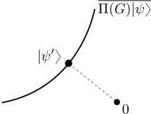
Figure 2.1: In the closure of an orbit $\Pi(G)\ket{\psi}$ for the complexified group $G$, any non-zero vector of minimal norm $\ket{\psi^{\prime}}$ gives rise to a pure state with maximally mixed marginals. Section 2.2 shows that a converse is also true.

Projective Space

Mathematically, the set of pure states on a Hilbert space $\mathcal{H}$,

$$\mathbbm{P}(\mathcal{H})=\{\rho=\lvert\psi\rangle\langle\psi\rvert:\braket{\psi}{\psi}=1\},$$

is known as a complex projective space. It is a smooth submanifold of the real vector space of Hermitian operators on $\mathcal{H}$. The unitary group $\operatorname{U}(\mathcal{H})$ acts transitively by conjugation, $U\lvert\psi\rangle\langle\psi\rvert U^{\dagger}$, so that the tangent space at a point $\rho=\lvert\psi\rangle\langle\psi\rvert$ is spanned by the tangent vectors $X_{\rho}=[X,\rho]$ for all $X\in\mathfrak{u}(\mathcal{H})$. Since the $X$ are anti-Hermitian, it is easy to verify that the tangent space can be equivalently written as

$$T_{\rho}\mathbbm{P}(\mathcal{H})=\{V=\lvert\phi\rangle\langle\psi\rvert+\lvert\psi\rangle\langle\phi\rvert:\ket{\phi}\in\mathcal{H},\braket{\phi}{\psi}=0\}\cong\ket{\psi}^{\perp}\subseteq\mathcal{H}.$$ (2.8)

In this way, the tangent space acquires a complex structure, which can be written as

$$J[V]=i[V,\rho]=i(\lvert\phi\rangle\langle\psi\rvert-\lvert\psi\rangle\langle\phi\rvert),$$

as well as a Hermitian inner product. The real part of the inner product is a Riemannian metric, $g(V,W)=\operatorname{tr}VW$, and its imaginary part is the Fubini–Study symplectic form

$$\omega(V,W)=g(J[V],W)=\operatorname{tr}J[V]W=-i\operatorname{tr}\rho[V,W].$$ (2.9)

For tangent vectors generated by elements of the Lie algebra $\mathfrak{u}(\mathcal{H})$, this becomes

$$\omega(X_{\rho},Y_{\rho})=-i\operatorname{tr}\rho[X_{\rho},Y_{\rho}]=i\operatorname{tr}\rho[X,Y]\quad(\forall X,Y\in\mathfrak{u}(\mathcal{H})).$$ (2.10)

The action of $\operatorname{U}(\mathcal{H})$ can be extended to its complexification, the general linear group $\operatorname{GL}(\cal H)$ by the formula

$$g\cdot\lvert\psi\rangle\langle\psi\rvert:=g\lvert\psi\rangle\langle\psi\rvert g^{\dagger}/\braket{\psi}{g^{\dagger}g}{\psi}.$$ (2.11)

The tangent vector generated by a Hermitian matrix $iX\in i\mathfrak{u}(\mathcal{H})$ is then given by $(iX)_{\rho}:=\{iX,\rho\}-2(\operatorname{tr}iX\rho)\rho$, with $\{A,B\}:=AB+BA$ the anti-commutator. It is easily verified that $(iX)_{\rho}=J[X_{\rho}]$. Thus the complex structures of projective space and of the Lie group are compatible with each other.

The Moment Map

Let $K$ be a compact connected Lie group, $G$ its complexification, and $\Pi\colon G\rightarrow\operatorname{GL}(\mathcal{H})$ a representation on a Hilbert space $\mathcal{H}$ with a $K$-invariant inner product; we denote the infinitesimal representation by $\pi\colon\mathfrak{g}\rightarrow\mathfrak{gl}(\mathcal{H})$. Then $K$ and $G$ also act on the projective space $\mathbbm{P}(\mathcal{H})$, and as in (2.11) we will denote this action by $g\cdot\rho$. The following is our basic object of interest:

Definition .

The moment map for the action of $K$ on $\mathbbm{P}(\mathcal{H})$ is defined by

$$\mu_{K}\colon\mathbbm{P}(\mathcal{H})\rightarrow i\mathfrak{k}^{*},\quad(\mu_{K}(\rho),X):=\operatorname{tr}\rho\,\pi(X)$$ (2.12)

for all $\rho\in\mathbbm{P}(\mathcal{H})$ and $X\in\mathfrak{g}$. Here and in the following, we write $(\varphi,X)=\varphi(X)$ for the pairing between $\mathfrak{g}^{*}$ and $\mathfrak{g}$.

Unfortunately, there are as many conventions for the moment map as there are textbooks on the subject. For the representation $\mathcal{H}$ that we considered at the beginning of this section, the moment map maps pure states onto the functionals evaluating (traceless) local observables; cf. (2.7). Thus the one-body quantum marginal problem is equivalent to characterizing the image of a moment map. In Section 2.3 we will explain this connection in more detail.

A crucial property of the moment map is the following relation between the differential of its components and the tangent vector $X_{\rho}=[\pi(X),\rho]$ generated by the infinitesimal action of the Lie algebra of the compact group:

$$d(\mu_{K},iX)\big{|}_{\rho}=\omega(X_{\rho},-)\quad(\forall X\in\mathfrak{k})$$ (2.13)

This follows readily from (2.10). Since the Fubini–Study form is non-degenerate, an immediate consequence is that the component (2.13) of the differential vanishes if and only if $X_{\rho}=0$. Dually, we find that the range of the differential of the moment map at any point $\rho$ is given by the annihilator of $\mathfrak{k}_{\rho}:=\{X\in\mathfrak{k}:X_{\rho}=[\pi(X),\rho]=0\}$, the Lie algebra of the $K$-stabilizer of $\rho$ [GS82a]:

$$d\mu_{K}\big{(}T_{\rho}\mathbbm{P}(\mathcal{H}))=\{\lambda\in i\mathfrak{k}^{*}:\lambda\big{|}_{i\mathfrak{k}_{\rho}}\equiv 0\}$$ (2.14)

This holds even if we restrict to the tangent space of the $G$-orbit through $\rho$, which is a complex submanifold and in particular symplectic (i.e., the Fubini–Study form $\omega$ remains non-degenerate). A second important property is that the moment map is $K$-equivariant: Indeed, for all $\rho\in\mathbbm{P}(\mathcal{H})$, $g\in K$ and $X\in i\mathfrak{k}$ we have that

$$(\mu_{K}(g\cdot\rho),X)=\operatorname{tr}\pi(g)\rho\,\pi(g^{-1})\pi(X)=\operatorname{tr}\rho\,\pi(g^{-1})\pi(X)\pi(g)$$

$$= \operatorname{tr}\rho\,\pi(\operatorname{Ad}(g^{-1})X)=(\mu_{K}(\rho),\operatorname{Ad}(g^{-1})X)=(\operatorname{Ad}^{*}(g)\mu_{K}(\rho),X).$$

Thus its image consists of a union of coadjoint orbits, and so is characterized by its intersection with the positive Weyl chamber $i\mathfrak{t}^{*}_{+}$. In the context of the quantum marginal problem, this amounts to our previous observation that its solution depends only on the eigenvalues of the one-body reduced density matrices.

The notion of a moment map can be defined more generally in symplectic geometry, and originates in Hamiltonian mechanics. For example, the function sending a point in the classical phase space $\mathbbm{R}^{6n}$ to the total linear and angular momentum is a moment map in this more general sense for the canonical action of the Euclidean group (see, e.g., [GS84b, CdS08]).

Our basic argument above showed that any non-zero vector of minimal length in an orbit closure has expectation value zero with respect to all local traceless observables (i.e., the image under the moment map is zero). The following result by Kempf and Ness shows a converse [KN79] (cf. [Kem78, NM84] and Figure 2.1 for an illustration).

Lemma (Kempf–Ness).

Let $\rho=\lvert\psi\rangle\langle\psi\rvert\in\mathbbm{P}(\mathcal{H})$ with $\mu_{K}(\rho)=0$. Then the $G$-orbit through $\ket{\psi}$ is closed (so in particular contains a non-zero vector of minimal length).

Proof.

Suppose for the sake of finding a contradiction that the $G$-orbit through $\ket{\psi}$ is not closed. Then the Hilbert–Mumford criterion asserts that we can reach a point in the “boundary” $\overline{\Pi(G)\ket{\psi}}\setminus\Pi(G)\ket{\psi}$ by using a single one-parameter subgroup (e.g., [Kra85, p. 171]). More formally, it states that there exists $X\in i\mathfrak{k}$ such that

$$\lim_{t\rightarrow\infty}\exp(\pi(X)t)\ket{\psi}=\ket{\psi^{\prime}}\not\in\Pi(G)\ket{\psi}.$$ (2.15)

Let $\ket{\psi}=\sum_{k}\ket{\psi_{k}}$ be the decomposition of $\ket{\psi}$ into eigenvectors of the Hermitian operator $\pi(X)$, with $\ket{\psi_{k}}$ an eigenvector with eigenvalue $k$. Clearly, $\ket{\psi_{k}}=0$ for all $k>0$, since otherwise the limit (2.15) cannot exist. But then

$$\sum_{k\leq 0}k\braket{\psi_{k}}{\psi_{k}}=\braket{\psi}{\pi(X)}{\psi}=(\mu_{K}(\rho),X)=0,$$

so that $\ket{\psi_{k}}=0$ also for all $k<0$. It follows that $\ket{\psi}=\ket{\psi_{0}}$, i.e. $\pi(X)\ket{\psi}=0$. Thus the one-parameter subgroup in fact leaves the vector invariant,

$$\exp(\pi(X)t)\ket{\psi}\equiv\ket{\psi}\quad(\forall t).$$

This is the desired contradiction to (2.15). ∎

In the following we need to study the image of the moment map not only for the set of all pure states but also for certain subsets of projective space. In the context of algebraic geometry, it is natural to consider $G$-invariant projective subvarieties, which we define in the following way (e.g., [Har77]):

Definition .

An affine cone $\mathcal{C}\subseteq\mathcal{H}$ is the common zero set of a family of homogeneous polynomials. The ring of regular functions $R(\mathcal{C}):=\bigoplus_{k=0}^{\infty}R_{k}(\mathcal{C})$ is defined as the ring of polynomials on $\mathcal{H}$, graded by the degree $k$, where we identify any two polynomials if their difference vanishes on $\mathcal{C}$. An affine cone is called irreducible if the ring of regular functions does not have any zero divisors (i.e. if for any two $P,Q\in R(\mathcal{C})$, $PQ=0$ implies that $P=0$ or $Q=0$). Finally, a projective subvariety of $\mathbbm{P}(\mathcal{H})$ is a set of the form

$$\mathbbm{X}=\mathbbm{P}(\mathcal{C}):=\{\lvert\psi\rangle\langle\psi\rvert:\ket{\psi}\in\mathcal{C},\braket{\psi}{\psi}=1\}\subseteq\mathbbm{P}(\mathcal{H}),$$

where $\mathcal{C}\subseteq\mathcal{H}$ is an irreducible affine cone. In this case, we also write $R(\mathbbm{X}):=R(\mathcal{C})$. We say that $\mathbbm{X}$ is $G$-invariant if $\Pi(G)\mathcal{C}\subseteq\mathcal{C}$ or, equivalently, if $G\cdot\mathbbm{X}\subseteq\mathbbm{X}$.

By definition, projective subvarieties are always closed in the Zariski topology of projective space, whose closed sets are common zero sets of families of homogeneous polynomials. Zariski-closed sets are also closed in the usual topology of projective space as a manifold, but the converse is not necessarily true. However, orbits $G\cdot\rho=\{g\cdot\rho:g\in G\}$ of algebraic group actions are constructible and hence the usual closure and the Zariski closure coincide (e.g., [Hum98, Proposition 8.3] and [SW05, Lemma 12.5.3]). In fact, any orbit closure $\overline{G\cdot\rho}$ is a $G$-invariant projective subvariety of $\mathbbm{P}(\mathcal{H})$ in the sense just defined (since our groups $G$ are connected).

For any $G$-invariant projective subvariety $\mathbbm{X}$, the ring of regular functions $R(\mathbbm{X})$ becomes a $G$-representation in a natural way: For each $g\in G$ and $P\in R(\mathbbm{X})$, we may define $\Pi(g)P$ by $(\Pi(g)P)(\ket{\psi}):=P(\Pi(g^{-1})\ket{\psi})$. In the language that we have just introduced, the basic argument given at the beginning of the section can be succinctly summarized as follows (together with its converse):

Lemma .

For any $G$-invariant projective subvariety $\mathbbm{X}\subset\mathbbm{P}(\mathcal{H})$, we have

$$R(\mathbbm{X})^{G}\neq\mathbbm{C}\quad\Leftrightarrow\quad 0\in\mu_{K}(\mathbbm{X}),$$

where $\mathbbm{C}$ stands for the constant functions.

Proof.

$(\Rightarrow)$ is proved just as at the beginning of this section: Let $\mathbbm{X}=\mathbbm{P}(\mathcal{C})$ and $P\in R_{k}(\mathbbm{X})^{G}$ a non-constant $G$-invariant homogeneous polynomial with $P(\ket{\psi})\neq 0$ for some $\ket{\psi}\in\mathcal{C}$. Since $P(0)=0$, $\overline{\Pi(G)\ket{\psi}}\not\ni 0$, hence we can find a non-zero vector $\ket{\psi^{\prime}}\in\overline{\Pi(G)\ket{\psi}}\subseteq\mathcal{C}$ of minimal length. In particular, $\ket{\psi^{\prime}}$ is of minimal length in its $G$-orbit, so that for all $X\in i\mathfrak{k}$ and using that $\pi(X)=\pi(X)^{\dagger}$ we find that

$$0=\partial_{t=0}\lVert\exp(\pi(X)t)\psi^{\prime}\rVert^{2}=2\braket{\psi^{\prime}}{\pi(X)}{\psi^{\prime}}.$$

Thus $\rho:=\lvert\psi^{\prime}\rangle\langle\psi^{\prime}\rvert/\braket{\psi^{\prime}}{\psi^{\prime}}\in\mathbbm{X}$ is a pure state with $\mu_{K}(\rho)=0$.

$(\Leftarrow)$ For any $\rho=\lvert\psi\rangle\langle\psi\rvert$ with $\mu_{K}(\rho)=0$, Section 2.2 asserts that the $G$-orbit through $\ket{\psi}$ is closed, so in particular it is disjoint from $\{0\}$. Since orbits are constructible in the sense of algebraic topology, their closure in the Hilbert space topology coincides with their closure in the Zariski topology, which is the topology whose closed sets are common zero sets of families of polynomials. But any two disjoint Zariski-closed sets can be separated by a polynomial: Hilbert’s Nullstellensatz implies that we may find a polynomial $P$ that separates $\Pi(G)\ket{\psi}$ and $\{0\}$ such that $P(\Pi(G)\ket{\psi})\equiv 1$ while $P(0)=0$ [Har77]. Without loss of generality, $P$ is homogeneous, and we may also average over $K$ to make it $G$-invariant. Then $P$ is a non-constant regular function in $R(\mathbbm{X})^{G}$. ∎

To generalize Section 2.2 to arbitrary points in the image of the moment map, we need as the last ingredient the Borel–Weil theorem (see, e.g., [VB11, Lemma 94]).

Lemma (Borel–Weil).

Let $V_{G,\lambda}$ be the irreducible $G$-representation with highest weight $\lambda\in\Lambda^{*}_{G,+}$ and highest weight vector $\ket{\lambda}$. Let $\mathbbm{X}_{G,\lambda}:=K\cdot\lvert\lambda\rangle\langle\lambda\rvert$. Then $\mathbbm{X}_{G,\lambda}=G\cdot\lvert\lambda\rangle\langle\lambda\rvert=\overline{G\cdot\lvert\lambda\rangle\langle\lambda\rvert}$ is a $G$-invariant projective subvariety of $\mathbbm{P}(V_{G,\lambda})$ for which

$$R_{k}(\mathbbm{X}_{G,\lambda})\cong V_{G,k\lambda}^{*}\quad\text{and}\quad\mu_{K,\lambda}(\lvert\lambda\rangle\langle\lambda\rvert)=\lambda,$$ (2.16)

where $\mu_{K,\lambda}$ denotes the moment map for $K$-action on $\mathbbm{P}(V_{G,\lambda})$. In fact, the moment map is a bijection between the projective subvariety $\mathbbm{X}_{G,\lambda}$ and its image, which is the coadjoint orbit $\mathcal{O}_{K,\lambda}$.

The Moment Polytope

The following proposition formalizes the fundamental link between the image of the moment map and the decomposition of the ring of regular functions into irreducible representations [GS82b, NM84, Bri87].

Proposition .

Let $\mathbbm{X}$ be a $G$-invariant projective subvariety of $\mathbbm{P}(\mathcal{H})$. Then:

$$\mu_{K}(\mathbbm{X})\cap\mathbbm{Q}\Lambda^{*}_{G,+}=\left\{\frac{\lambda}{k}:V^{*}_{G,\lambda}\subseteq R_{k}(\mathbbm{X})\right\}$$

Proof.

Fix $\lambda\in\Lambda^{*}_{G,+}$ and $k>0$. Let $\widetilde{\mathcal{H}}:=\operatorname{Sym}^{k}(\mathcal{H})\otimes V_{G,\lambda^{*}}$. Then

$$\widetilde{\mathbbm{X}}:=\{\lvert\psi\rangle\langle\psi\rvert^{\otimes k}\otimes\lvert\phi\rangle\langle\phi\rvert:\lvert\psi\rangle\langle\psi\rvert\in\mathbbm{X},\lvert\phi\rangle\langle\phi\rvert\in\mathbbm{X}_{G,\lambda^{*}}\}$$

is a projective subvariety of $\mathbbm{P}(\widetilde{\mathcal{H}})$ – known as the image of the product of the $k$-th Veronese embedding of $\mathbbm{X}$ and $\mathbbm{X}_{G,\lambda^{*}}$ under the Segré embedding – and it is not hard to see that its ring of regular functions is given by

$$R_{l}(\widetilde{\mathbbm{X}})\cong R_{kl}(\mathbbm{X})\otimes R_{l}(\mathbbm{X}_{G,\lambda^{*}})\cong R_{kl}(\mathbbm{X})\otimes V_{G,\lambda l},$$

where we have used the first assertion in (2.16). Thus, $R_{l}(\widetilde{\mathbbm{X}})^{G}\neq 0$ if and only if $V_{G,\lambda l}^{*}\subseteq R_{kl}(\mathbbm{X})$.

On the other hand, the infinitesimal action of $\mathfrak{g}$ on $\widetilde{\mathcal{H}}$ is $\widetilde{\pi}(X)=k\,\pi(X)\otimes\mathbbm{1}_{V_{G,\lambda}}+\mathbbm{1}_{\mathcal{H}}\otimes\pi_{\lambda^{*}}(X)$, with $\pi_{\lambda^{*}}$ the irreducible representation of $\mathfrak{g}$ on $V_{G,\lambda}$. Hence the moment map on $\widetilde{\mathbbm{X}}$ is given by the formula

$$\widetilde{\mu}_{K}(\lvert\psi\rangle\langle\psi\rvert^{\otimes k}\otimes\lvert\phi\rangle\langle\phi\rvert)=k\,\mu_{K}(\lvert\psi\rangle\langle\psi\rvert)+\mu_{K,\lambda^{*}}(\lvert\phi\rangle\langle\phi\rvert).$$

It follows by using the second assertion in (2.16) and $\lambda^{*}=-w_{0}\lambda$ that

$$\widetilde{\mu}_{K}(\widetilde{\mathbbm{X}})=k\,\mu_{K}(\mathbbm{X})+\mathcal{O}_{K,\lambda^{*}}=k\,\mu_{K}(\mathbbm{X})-\mathcal{O}_{K,\lambda},$$ (2.17)

hence $0\in\widetilde{\mu}_{K}(\widetilde{\mathbbm{X}})$ if and only if $\lambda/k\in\mu_{K}(\mathbbm{X}))$. The theorem follows from these two observations and Section 2.2. ∎

It is instructive to apply Section 2.2 to the situation of Section 2.2.

Proposition .

Let $\mathbbm{X}$ be a $G$-invariant projective subvariety of $\mathbbm{P}(\mathcal{H})$. Then $\{(\lambda,k):V^{*}_{G,\lambda}\subseteq R_{k}(\mathbbm{X})\}$ is a finitely generated semigroup. It follows that $\{\lambda/k:V^{*}_{G,\lambda}\subseteq R_{k}(\mathbbm{X})\}$ is a convex polytope over $\mathbbm{Q}$.

Proof.

Set $\mathcal{S}:=\{(\lambda,k):V^{*}_{G,\lambda}\subseteq R_{k}(\mathbbm{X})\}$. We first show that $\mathcal{S}$ is a semigroup, i.e., closed under addition. Recall from Section 2.1 that the highest weight vectors are in one-to-one correspondence with the irreducible representations that occur in a given representation. Thus let $P\in R_{k}(\mathbbm{X})$ and $Q\in R_{l}(\mathbbm{X})$ be highest weight vectors of weight $\lambda$ and $\mu\in\Lambda^{*}_{G,+}$ corresponding to two points $(\lambda,k)$ and $(\mu,l)\in\mathcal{S}$. We claim that their product $PQ$ is a highest weight vector of weight $\lambda+\mu$ in $R_{k+l}(\mathbbm{X})$. Indeed, $PQ\neq 0$ since $\mathbbm{X}$ is irreducible by assumption; it has weight $\lambda+\mu$ since

$$\pi(H)(PQ)=(\pi(H)P)Q+P(\pi(H)Q)=(\lambda(H)+\mu(H))PQ\quad(\forall H\in\mathfrak{h}),$$

and an analogous calculation shows that it is annihilated by $\mathfrak{n}_{+}$ and hence a highest weight vector. Thus we obtain the point $(\lambda+\mu,k+l)\in\mathcal{S}$. To see that $\mathcal{S}$ is finitely generated, we use the (highly non-trivial) fact that the algebra of $N_{+}$-invariants $R(\mathbbm{X})^{N_{+}}$, whose elements are linear combinations of highest weight vectors, is finitely generated [Gro73]. Let $P^{(1)},\dots,P^{(m)}$ be a finite set of generators; we may assume that each generator is homogeneous, say $P^{(j)}\in R_{k^{(j)}}(\mathbbm{X})^{N_{+}}$, and a weight vector, say of weight $\lambda^{(j)}$. Then $(\lambda^{(j)},k^{(j)})\in\mathcal{S}$ for all $j=1,\dots,m$. On the other hand, we find just as above that any monomial $P^{(j_{1})}\dotsm P^{(j_{p})}$ has degree $\sum_{i}k^{(j_{i})}$ and weight $\sum_{i}\lambda^{(j_{i})}$, and therefore determines the point $\sum_{i}(\lambda^{(j_{i})},k^{(j_{i})})\in\mathcal{S}$. Since any highest weight vector can then be written as a sum of monomials in the $P^{(j)}$, we conclude that $\mathcal{S}$ is a semigroup that is generated by the finitely many points $(\lambda^{(j)},k^{(j)})$ for $j=1,\dots,m$.

It follows as an immediate consequence that

$$\mathcal{P}:=\{\lambda/k:V^{*}_{G,\lambda}\subseteq R_{k}(\mathbbm{X})\}=\{\lambda/k:(\lambda,k)\in\mathcal{S}\}$$

is a convex polytope over $\mathbbm{Q}$. Indeed, let $(\lambda,k)$ and $(\mu,l)\in\mathcal{S}$ corresponding to two points $\lambda/k$ and $\mu/l\in\mathcal{P}$. Then $pl(\lambda,k)+qk(\mu,l)\in\mathcal{S}$ by the semigroup property, so that we obtain the point

$$\frac{pl\lambda+qk\mu}{plk+qkl}=\frac{p}{p+q}\frac{\lambda}{k}+\frac{q}{p+q}\frac{\mu}{l}\in\mathcal{P}.$$

Thus $\mathcal{P}$ is closed under convex combinations with rational coefficients. Likewise, the fact that $\mathcal{S}$ is generated by the finitely many generators $(\lambda^{(j)},k^{(j)})$ implies that $\mathcal{P}$ is the convex hull over $\mathbbm{Q}$ of the finitely many points $\lambda^{(j)}/k^{(j)}$ ($j=1,\dots,m$). ∎

For any $(\lambda,k)$ in the semigroup, its integral multiples $\mathbbm{Z}_{>0}(\lambda,k)$ are also contained in the semigroup, and they determine the same point $\lambda/k$ in the polytope. Therefore, the polytope only depends on the representation theory of $R_{k}(\mathbbm{X})$ in the “semiclassical limit” of large $k$:

$$\left\{\frac{\lambda}{k}:V^{*}_{G,\lambda}\subseteq R_{k}(\mathbbm{X})\right\}=\left\{\frac{\lambda}{k}:V^{*}_{G,\lambda}\subseteq R_{k}(\mathbbm{X}),k\geq k_{0}\right\}\quad(\forall k_{0}>0)$$ (2.18)

It is well-known that $\mu_{K}(\mathbbm{X})\cap\mathbbm{Q}\Lambda^{*}_{G,+}$ is a dense subset of $\mu_{K}(\mathbbm{X})\cap i\mathfrak{t}^{*}_{+}$ (see, e.g., [GS82a, NM84]; this also follows from the local model for symplectic group actions, cf. the discussion below Section 2.3). By combining Section 2.2 and Section 2.2, we thus arrive at the following fundamental theorem:

Theorem 2.1 (Mumford).

Let $\mathbbm{X}$ be a $G$-invariant projective subvariety of $\mathbbm{P}(\mathcal{H})$. Then

$$\Delta_{K}(\mathbbm{X})=\mu_{K}(\mathbbm{X})\cap i\mathfrak{t}^{*}_{+}=\{\lambda\in i\mathfrak{t}^{*}_{+}:\mathcal{O}_{K,\lambda}\subseteq\mu_{K}(\mathbbm{X})\}$$

is a convex polytope with rational vertices, whose rational points are given by

$$\mu_{K}(\mathbbm{X})\cap\mathbbm{Q}\Lambda^{*}_{G,+}=\left\{\frac{\lambda}{k}:V^{*}_{G,\lambda}\subseteq R_{k}(\mathbbm{X})\right\}.$$

It is called the moment polytope for the $K$-action on $\mathbbm{X}$.

In the proof of Section 2.2 we had identified the irreducible representations that occur in $R(\mathbbm{X})$ with their highest weight vectors, which are precisely the weight vectors in $R(\mathbbm{X})^{N_{+}}$. From a conceptual point of view, the passage from highest weight vectors in $R(\mathbbm{X})$ to weight vectors in $R(\mathbbm{X})^{N_{+}}$ is a first instance of the reduction of a non-Abelian problem to an Abelian problem as alluded to in the abstract of this thesis. It also leads to a basic way of computing the moment polytope $\Delta_{K}(\mathbbm{X})$ (cf. the discussion at the end of Section 4.3). In the next chapters we will meet more refined variants of this reduction.

The study of moment maps and their convexity properties has a long history in mathematics. Among the well-known special cases are: The Schur–Horn theorem concerning the diagonal entries of Hermitian matrices with fixed spectrum [Sch23, Hor54]; Kostant’s convexity theorem, which is the generalization to general coadjoint orbits [Kos73]; the Atiyah–Guillemin–Sternberg convexity theorem for torus actions [Ati82, GS82a]; Heckman’s convexity theorem, which considers projections of coadjoint orbits [Hec82]; and Kirwan’s convexity theorem, which is the symplectic analogue of Theorem 2.1 [Kir84b] (cf. [Sja98, Bri99] and the recent monograph [GS05]).

2.3 Consequences for the Quantum Marginal Problem

We now describe the precise connection between the geometry of the moment map and the one-body quantum marginal problem and draw some general consequences.

For distinguishable particles, consider the Hilbert space $\mathcal{H}=\bigotimes_{k=1}^{n}\mathcal{H}_{k}$ equipped with the representation of $G=\operatorname{GL}(\mathcal{H}_{1})\times\dots\times\operatorname{GL}(\mathcal{H}_{n})$ by tensor products, $\Pi(g_{1},\dots,g_{n})=g_{1}\otimes\dots\otimes g_{n}$. Its Lie algebra $\mathfrak{g}=\mathfrak{gl}(\mathcal{H}_{1})\oplus\dots\oplus\mathfrak{gl}(\mathcal{H}_{n})$ acts by $\pi(X_{1},\dots,X_{n})=\sum_{k=1}^{n}\mathbbm{1}^{\otimes k-1}\otimes X_{k}\otimes\mathbbm{1}^{\otimes n-k}$. The group $K=\operatorname{U}(\mathcal{H}_{1})\times\dots\times\operatorname{U}(\mathcal{H}_{n})$ is a maximal compact subgroup of $G$ and it acts unitarily on $\mathcal{H}$. For all tuples of Hermitian matrices $X=(X_{1},\dots,X_{n})\in i\mathfrak{k}$, the moment map (2.12) is given by

$$(\mu_{K}(\rho),X)=\sum_{k=1}^{n}\operatorname{tr}\rho(\mathbbm{1}^{\otimes k-1}\otimes X_{k}\otimes\mathbbm{1}^{\otimes n-k})=\sum_{k=1}^{n}\operatorname{tr}\rho_{k}X_{k},$$

where we have used the definition (2.1) of the one-body reduced density matrices $\rho_{k}$. Thus if we identify each $\rho_{k}$ with its dual, $\operatorname{tr}\rho_{k}(-)$, then the one-body quantum marginal problem, Chapter 2, is precisely equivalent to characterizing the image of the moment map. Furthermore, the moment polytope $\Delta_{K}(\mathbbm{P}(\mathcal{H}))=\mu_{K}(\mathbbm{P}(\mathcal{H}))\cap i\mathfrak{t}^{*}_{+}$ can be identified with the collection of eigenvalues $(\vec{\lambda}_{1},\dots,\vec{\lambda}_{n})$ of the one-body reduced density matrices $\rho_{1},\dots,\rho_{n}$ that are compatible with a global pure state $\rho\in\mathbbm{P}(\mathcal{H})$:

$$\Delta_{K}(\mathbbm{P}(\mathcal{H}))=\left\{(\vec{\lambda}_{1},\dots,\vec{\lambda}_{n}):\vec{\lambda}_{k}=\operatorname{spec}\rho_{k},\rho\in\mathbbm{P}(\mathcal{H})\right\},$$

where we identify diagonal matrices with non-increasing entries with their spectrum (as in Section 2.1 and Table 2.1).

In practice, the above modeling of the quantum marginal problem has the disadvantage that the moment polytope is always of positive codimension: since $\operatorname{tr}\rho_{k}\equiv\operatorname{tr}\rho=1$, $\Delta_{K}$ is contained in the affine subspace $\sum_{j}\lambda_{k,j}=1$ for all $k=1,\dots,n$. It will usually be more convenient to instead use the special linear and unitary groups, $G=\operatorname{SL}(\mathcal{H}_{1})\times\dots\times\operatorname{SL}(\mathcal{H}_{n})$ and $K=\operatorname{SU}(\mathcal{H}_{1})\times\dots\times\operatorname{SU}(\mathcal{H}_{n})$, so that $i\mathfrak{k}$ consists of tuples of traceless Hermitian matrices. Then the moment map preserves only the traceless part of the one-body reduced density matrices, which avoids the above degeneracy.

For fermions, we similarly choose $\mathcal{H}=\bigwedge^{n}\mathcal{H}_{1}$ and $G=\operatorname{SL}(\mathcal{H}_{1})$ acting by $\Pi(g_{1})=g_{1}^{\otimes n}$. With $K=\operatorname{SU}(\mathcal{H}_{1})$ and using (2.3) we obtain that

$$(\mu_{K}(\rho),X_{1})=\sum_{k=1}^{n}\operatorname{tr}\rho(\mathbbm{1}^{\otimes k-1}\otimes X_{k}\otimes\mathbbm{1}^{\otimes n-k})=n\operatorname{tr}\rho_{1}X_{1}=\operatorname{tr}\gamma_{1}X_{1},$$

where $\gamma_{1}:=n\rho_{1}$ is the first-order density matrix from quantum chemistry with trace $n$ that we had defined below (2.3). Again we find that the one-body $n$-representability problem, Chapter 2, is precisely equivalent to determining the moment polytope.

We can similarly model the other variants of the one-body quantum marginal problem alluded to at the end of the introduction of this chapter by considering different representations of unitary groups or their composition. For example, if $\mathcal{H}_{0}$ is a $K_{0}$-representation describing a pure-state problem then the corresponding mixed-state problem can be studied by taking $\mathcal{H}=\mathcal{H}_{0}\otimes\mathcal{H}_{0}$ and $K=K_{0}\times\operatorname{SU}(\mathcal{H}_{0})$; e.g., the mixed-state problem for fermions amounts to the moment polytope for the $\operatorname{SU}(\mathcal{H}_{1})\otimes\operatorname{SU}(\bigwedge^{n}\mathcal{H}_{1})$-representation $\bigwedge^{n}\mathcal{H}_{1}\otimes\bigwedge^{n}\mathcal{H}_{1}$. In Section 3.4 we discuss another example that involves the marginal problem for the spin and orbital degrees of freedom of a fermionic system. In Table 2.3 we summarize the mathematical modeling of the scenarios of main physical interest.

Setting	Group $K$	Representation $\mathcal{H}$
Distinguishable particles	$\bigtimes_{k=1}^{n}\operatorname{SU}(\mathcal{H}_{k})$	$\bigotimes_{k=1}^{n}\mathcal{H}_{k}$
Fermions	$\operatorname{SU}(\mathcal{H}_{1})$	$\bigwedge^{n}\mathcal{H}_{1}$
Bosons	$\operatorname{SU}(\mathcal{H}_{1})$	$\operatorname{Sym}^{n}\mathcal{H}_{1}$
Mixed-state version of $(\mathcal{H}_{0},K_{0})$	$K_{0}\times\operatorname{SU}(\mathcal{H}_{0})$	$\mathcal{H}_{0}\otimes\mathcal{H}_{0}$

Table 2.3: The different variants of the one-body quantum marginal problem can all be modeled by studying the moment polytope $\Delta_{K}(\mathbbm{P}(\mathcal{H}))$ for the action of a compact Lie group $K$ on the complex projective space of a $K$-representation $\mathcal{H}$. The table lists some important scenarios.

Convexity

For all these variants of the one-body quantum marginal problem, Theorem 2.1 immediately implies that the solution is given by a convex polytope, i.e., by linear inequalities on the eigenvalues of the one-body reduced density matrices. For example, Pauli’s original exclusion principle is one such inequality—but in general there are many further constraints. As we will see in several concrete examples in Chapter 3, there is a rich variety of subtle kinematic constraints on the one-body marginals of a multipartite quantum state.

To compute the actual linear inequalities for a given number of particles, statistics and local dimensions is in general a difficult problem that we will study in the next chapter. All known general solutions rely in one way or the other on the invariant-theoretic description of the moment polytope given by Theorem 2.1, including the original solution by Klyachko [Kly04] and the solution that we present in Chapter 3. In the remainder of this section we discuss the physical significance of the facets of the moment polytope, and we then describe more explicitly the representation-theoretic content of Theorem 2.1.

Pinning

An important consequence of the general theory is that the facets of the polytope have a rather particular structure. Before we show this, we record the following useful lemma for future reference.

Lemma .

Let $\rho\in\mathbbm{P}(\mathcal{H})$ such that $\mu_{K}(\rho)\in i\mathfrak{t}^{*}_{>0}$ and $V\in d\mu_{K}^{-1}\big{|}_{\rho}(i\mathfrak{t}^{*})$. Then there exists a smooth curve $\rho_{t}\in\mathbbm{P}(\mathcal{H})$ for $t\in(-\varepsilon,\varepsilon)$ such that

$$\rho_{0}=\rho,\quad\dot{\rho}_{0}=V,\quad\text{and}\quad\mu_{K}(\rho_{t})\in i\mathfrak{t}^{*}_{>0}\;(\forall t).$$

Proof.

Consider the symplectic cross section $Y:=\mu_{K}^{-1}(i\mathfrak{t}^{*}_{>0})$. By $K$-equivariance of the moment map, $\mu_{K}$ meets $i\mathfrak{t}^{*}_{>0}$ transversally, so that $Y$ is a smooth manifold with tangent space $T_{\rho}Y=d\mu_{K}^{-1}\big{|}_{\rho}(i\mathfrak{t}^{*})$ [GS84b, Theorem 26.7]. Thus we may choose any curve in $Y$ that starts with $\rho_{0}=0$ and $\dot{\rho}_{0}=V$. ∎

In the context of the marginal problem, Section 2.3 is in essence a reformulation of first-order perturbation theory for the one-body reduced density matrices. We remark that its conclusions can be strengthened; it is in fact possible to walk “finitesimally” into any direction in $d\mu_{K}(T_{\rho}\mathbbm{P}(\mathcal{H}))\cap i\mathfrak{t}^{*}$, as can be seen by using the local model for symplectic group actions [GS82a, GS84a, Mar85].

Lemma (Selection Rule).

Let $\rho=\lvert\psi\rangle\langle\psi\rvert$ be a pure state such that $\mu_{K}(\rho)\in i\mathfrak{t}^{*}_{>0}$ is a point on a facet of the moment polytope corresponding to the inequality $(-,H)\geq c$. Then

$$d(\mu_{K},H)\big{|}_{\rho}=0$$

and

$$\pi(H)\ket{\psi}=c\ket{\psi}.$$ (2.19)

Proof.

For any $\omega\in d\mu_{K}(T_{\rho}\mathbbm{P}(\mathcal{H}))\cap i\mathfrak{t}^{*}$, there exists a curve $\rho_{t}$ through $\mu_{K}(\rho)$ with $d\mu_{K}(\dot{\rho}_{0})=\omega$ and $\mu_{K}(\rho_{t})\in\Delta_{K}$ for all $t$ (Section 2.3). Therefore,

$$(\mu_{K}(\rho_{t}),H)=c+t(\omega,H)+O(t^{2}).$$

Since $(\mu_{K}(\rho_{t}),H)\geq c$ is an inequality for the moment polytope, it follows that $(\omega,H)=0$—for otherwise we could walk through the facet! On the other hand, (2.14) shows that

$$d\mu_{K}\big{(}T_{\rho}\mathbbm{P}(\mathcal{H}))\cap i\mathfrak{t}^{*}=\{\omega\in i\mathfrak{t}^{*}:\omega\big{|}_{i\mathfrak{k}_{\rho}}=0\}=\{\omega\in i\mathfrak{t}^{*}:\omega\big{|}_{i\mathfrak{t}_{\rho}}=0\}.$$

Therefore, $H\in i\mathfrak{t}$ is necessarily an element of the Lie algebra of the $T$-stabilizer of $\rho$, i.e., $H_{\rho}=[\pi(H),\rho]=0$. This implies that $d(\mu_{K},H)\big{|}_{\rho}=0$ by (2.13), but also that $\ket{\psi}$ is an eigenvector of $\pi(H)$, with corresponding eigenvalue $\braket{\psi}{\pi(H)}{\psi}=(\mu_{K}(\rho),H)=c$. ∎

In the language of Klyachko, the eigenvalue equation (2.19) is called the selection rule which is satisfied by a quantum state that is pinned to a facet of the moment polytope [Kly09]. Thus pinned states live on a potentially much lower-dimensional subspace of the Hilbert space, with potential implications on the physics.

It is an interesting question if and under which circumstances states in concrete systems are pinned. For example, it is an empirical fact that many molecules are well-explained by assuming that the natural occupation numbers are close to 0 and 1 (pinning), so that the global state can be well-approximated by a Slater determinant (the corresponding selection rule), which is a first step to Hartree–Fock theory and the Aufbau principle. Thus it is not be unreasonable to wonder if approximate pinning might hold for some of the other defining inequalities of the moment polytope. See [Kly09, Kly13] for preliminary investigations in the context of small molecules and magnetism and [SGC13] for a study of pinning in a model with small harmonic interactions.

Crucially, the selection rule is stable at least in an elementary sense. We phrase the following result in terms of the trace norm $\lVert X\rVert_{1}:=\operatorname{tr}\lvert X\rvert$, which has a useful operational meaning (but this choice is completely arbitrary since the proof is based on a purely topological argument):

Lemma (Stability).

Let $\lVert-\rVert$ denote an arbitrary norm on $i\mathfrak{t}^{*}$. Let $F=\{\lambda\in\Delta_{K}(\mathbbm{P}(\mathcal{H})):(\lambda,H)=c\}$ be a facet of the moment polytope and $\mathcal{H}(H=c)=\{\ket{\psi}:\pi(H)\ket{\psi}=\ket{\psi}c\}$ the corresponding subspace of states that satisfy the selection rule. For any closed subset $F_{0}\subseteq F\cap i\mathfrak{t}^{*}_{>0}$ there exists a function $\delta(\varepsilon)$ such that

$$\min_{\lambda\in F_{0}}\lVert\mu_{K}(\rho)-\lambda\rVert\leq\varepsilon\Rightarrow\min_{\rho^{\prime}\in\mathbbm{P}(\mathcal{H}(H=c))}\lVert\rho-\rho^{\prime}\rVert_{1}\leq\delta(\varepsilon)\qquad(\forall\rho)$$

and $\delta(\varepsilon)\searrow 0$ as $\varepsilon\searrow 0$.

Proof.

Set $F_{\varepsilon}:=\{\mu\in i\mathfrak{t}^{*}_{+}:\min_{\lambda\in F_{0}}\lVert\mu-\lambda\rVert\leq\varepsilon\}$. Each $F_{\varepsilon}$ is a closed set, hence $\mu_{K}^{-1}(F_{\varepsilon})$ is a compact subset of $\mathbbm{P}(\mathcal{H})$. Since moreover $d(\rho):=\min_{\rho^{\prime}\in\mathbbm{P}(\mathcal{H}(H=c))}\lVert\rho-\rho^{\prime}\rVert_{1}$ is continuous, it follows that the function

$$\delta(\varepsilon):=\max d(\mu_{K}^{-1}(F_{\varepsilon}))=\max\{\min_{\rho^{\prime}\in\mathbbm{P}(\mathcal{H}(H=c))}\lVert\rho-\rho^{\prime}\rVert_{1}:\rho\in\mathbbm{P}(\mathcal{H}),\mu_{K}(\rho)\in F_{\varepsilon}\}$$

is well-defined. Clearly, $\delta(\varepsilon)$ is monotonic in $\varepsilon$, and $\delta(0)=0$ by Section 2.3.

It remains to show that $\delta(\varepsilon)\rightarrow 0$ as $\varepsilon\rightarrow 0$. For sake of contradiction, suppose that this is not the case. Then there exists a sequence $(\rho_{k})\subseteq\mathbbm{P}(\mathcal{H})$ and $C>0$ such that $\min_{\lambda\in F_{0}}\lVert\mu_{K}(\rho_{k})-\lambda\rVert\rightarrow 0$ while $\delta(\rho_{k})\geq C$ for all $k$. By compactness, we may pass to a convergent subsequence; let us denote its limit by $\rho_{\infty}$. Then $\mu_{K}(\rho_{\infty})\in F_{0}$, while $\delta(\rho_{\infty})\geq C$. This is a contradiction to Section 2.3. ∎

For concrete applications, it might be interesting to obtain explicit bounds of the form $\delta(\varepsilon)\leq L\varepsilon$. So far this has only been achieved in rather special situations [SGC13, BRGBS13]. It might be possible to obtain a general solution by carefully analyzing the local model for symplectic group actions [GS82a, GS84a, Mar85].

2.4 Kronecker coefficients, Schur–Weyl duality, and Plethysms

In this section we describe more explicitly the representation-theoretic content of Theorem 2.1 for Problems 2 and 2.

We first consider the case of three distinguishable particles and choose coordinates, so that $\mathcal{H}=\mathbbm{C}^{a}\otimes\mathbbm{C}^{b}\otimes\mathbbm{C}^{c}$ and $G=\operatorname{SL}(a)\times\operatorname{SL}(b)\times\operatorname{SL}(c)$. For $\mathbbm{X}=\mathbbm{P}(\mathcal{H})$, the ring of regular functions is equal to the ring of all polynomials on $\mathcal{H}$, so that $R_{k}(\mathbbm{P}(\mathcal{H}))=\operatorname{Sym}^{k}(\mathcal{H})^{*}$. Thus we obtain from Theorem 2.1 the following description:

$$\Delta_{K}(\mathbbm{P}(\mathcal{H}))\cap\mathbbm{Q}\Lambda^{*}_{G,+} =\{(\alpha,\beta,\gamma)/k:V^{a}_{\alpha}\otimes V^{b}_{\beta}\otimes V^{c}_{\gamma}\subseteq\operatorname{Sym}^{k}(\mathbbm{C}^{abc})\}$$

$$=\{(\alpha,\beta,\gamma)/k:g_{\alpha,\beta,\gamma}>0\}.$$

where we denote by $g_{\alpha,\beta,\gamma}$ the multiplicity of $V^{a}_{\alpha}\otimes V^{b}_{\beta}\otimes V^{c}_{\gamma}$ in $\operatorname{Sym}^{k}(\mathbbm{C}^{abc})$. These multiplicities are known as the Kronecker coefficients.

There is another way of defining the Kronecker coefficients in terms of the symmetric groups $S_{k}$ that will be useful later. For this, we consider the space $(\mathbbm{C}^{d})^{\otimes k}$. The general linear group $\operatorname{GL}(d)$ acts diagonally by tensor powers and the symmetric group $S_{k}$ acts by permuting the tensor factors; both actions commute. Therefore, if we decompose $V$ into irreducible representations of $\operatorname{GL}(d)$ then the multiplicity spaces – which we shall denote by $[\lambda]$ – are representations of $S_{k}$. It can be shown that the irreducible $\operatorname{GL}(d)$-representations that appear are precisely those whose Young diagram $\lambda$ has $k$ boxes and at most $d$ rows. What is more, the corresponding representations $[\lambda]$ of the symmetric group are in fact irreducible. For each Young diagram, one obtains a different irreducible representation (which does not depend on the concrete value chosen for $d$), and all the irreducible representations of the symmetric group can be obtained in this way (if $d$ is large enough). This result is known as Schur–Weyl duality (e.g., [CSM95]) and it can be compactly stated in the form:

$$\left(\mathbbm{C}^{d}\right)^{\otimes k}\cong\;\smashoperator[]{\bigoplus_{\lambda\vdash_{d}k}^{}}\;V^{d}_{\lambda}\otimes[\lambda]$$ (2.20)

Now consider the tripartite case, where $d=abc$. Then the symmetric subspace $\operatorname{Sym}^{k}(\mathbbm{C}^{abc})\subseteq(\mathbbm{C}^{abc})^{\otimes k}$ corresponds to the trivial representation of $S_{k}$. On the other hand we may apply Schur–Weyl duality to each of the subsystems’ tensor powers,

$$(\mathbbm{C}^{abc})^{\otimes k}=(\mathbbm{C}^{a})^{\otimes k}\otimes(\mathbbm{C}^{b})^{\otimes k}\otimes(\mathbbm{C}^{c})^{\otimes k}=\;\smashoperator[]{\bigoplus_{\alpha\vdash_{a}k,\,\beta\vdash_{b}k,\,\gamma\vdash_{c}k}^{}}\;V^{a}_{\alpha}\otimes V^{b}_{\beta}\otimes V^{c}_{\gamma}\otimes[\alpha]\otimes[\beta]\otimes[\gamma]$$

It follows that

$$\operatorname{Sym}^{k}(\mathbbm{C}^{abc})=\;\smashoperator[]{\bigoplus_{\alpha\vdash_{a}k,\,\beta\vdash_{b}k,\,\gamma\vdash_{c}k}^{}}\;V^{a}_{\alpha}\otimes V^{b}_{\beta}\otimes V^{c}_{\gamma}\otimes\left([\alpha]\otimes[\beta]\otimes[\gamma]\right)^{S_{k}}$$ (2.21)

Thus the Kronecker coefficients can be equivalently defined as the dimension of the invariant subspace in a triple tensor product of irreducible representations of the symmetric group:

$$g_{\alpha,\beta,\gamma}=\dim\,\left([\alpha]\otimes[\beta]\otimes[\gamma]\right)^{S_{k}}$$

In particular, we find that each Kronecker coefficient only depends on the triple of Young diagrams rather than the concrete values chosen for $a$, $b$ and $c$ (but of course $a$, $b$ and $c$ have to be chosen at least as large as the number of rows of the Young diagrams). The role of the Kronecker coefficients for the one-body quantum marginal problem has first been observed in [CM06] by using the spectrum estimation theorem (cf. [Kly04, CHM07] and the proof of Theorem 9.1). They also play a fundamental role in representation theory [Ful97] and in Mulmuley and Sohoni’s geometric complexity theory approach to the $\mathbf{P}$ vs. $\mathbf{NP}$ problem in computer science [MS01, MS08, Mul07, BLMW11] (see Section 6.1), and they occur in the “quantum method of types” [Har05]. In Chapter 6 we will give an efficient algorithm for their computation.

There is a different, asymmetric way of defining the Kronecker coefficients that is also quite useful. For this, we recall that the irreducible representations of the symmetric group are self-dual, i.e., $[\lambda]\cong[\lambda]^{*}$ [JK81, §2.1]. Therefore,

$$([\alpha]\otimes[\beta]\otimes[\gamma])^{S_{k}}=([\alpha]^{*}\otimes[\beta]\otimes[\gamma])^{S_{k}}=\operatorname{Hom}_{S_{k}}([\alpha],[\beta]\otimes[\gamma]),$$

where we have used the general notation

$$\operatorname{Hom}_{G}(V,W):=\{\phi\colon V\rightarrow W\text{ linear}:\phi(gv)=g\phi(v)\quad(\forall v\in V,g\in G)\}$$ (2.22)

for the space of $G$-equivariant linear maps, or $G$-linear maps between two representations $V$ and $W$. For irreducible $V$ and $W$, Schur’s lemma asserts that

$$\dim\operatorname{Hom}_{S_{k}}(V,W)=\begin{cases}1&\text{if }V\cong W\\ 0&\text{otherwise}.\end{cases}$$ (2.23)

It follows that $g_{\alpha,\beta,\gamma}$ can also be defined as the multiplicity of $[\alpha]$ in the tensor product $[\beta]\otimes[\gamma]$ of two irreducible representations of the symmetric group:

$$[\beta]\otimes[\gamma]=\bigoplus_{\alpha\vdash k}g_{\alpha,\beta,\gamma}[\alpha]$$ (2.24)

In particular, for $[\gamma]=\mathbf{1}$ the trivial representation of $S_{k}$ we obtain that $g_{\alpha,\beta,\mathbf{1}}=\delta_{\alpha,\beta}$. In view of Schur–Weyl duality, this implies that

$$\operatorname{Sym}^{k}(\mathbbm{C}^{a}\otimes\mathbbm{C}^{b})=\;\smashoperator[]{\bigoplus_{\alpha\vdash_{a}k,\,\beta\vdash_{b}k}^{}}\;\delta_{\alpha,\beta}\,V^{a}_{\alpha}\otimes V^{b}_{\beta}=\;\smashoperator[]{\bigoplus_{\alpha\vdash_{\min\{a,b\}}k}^{}}\;V^{a}_{\alpha}\otimes V^{b}_{\alpha}.$$ (2.25)

This equation corresponds to the one-body quantum marginal problem for $n=2$ particles and is therefore the bipartite counterpart of (2.21). The fact that the irreducible representations of the two factors are perfectly paired is the representation-theoretic version of the fact that the marginals of a bipartite pure state are isospectral (Chapter 2)—indeed, the latter is a direct consequence of (2.25) and Theorem 2.1.

In the case of fermions, we are similarly led to study the decomposition of $R_{k}^{*}(\mathcal{H})=\operatorname{Sym}^{k}\left(\bigwedge^{n}\mathbbm{C}^{d}\right)$ into irreducible representations. This is an instance of a plethysm, which is more generally defined as the composition of Schur functors $\mathcal{H}\mapsto V_{\operatorname{GL}(\mathcal{H}),\lambda}$ (see, e.g., [Mac95]).

Sums of Matrices

We conclude this section by mentioning an interesting related problem that is amenable to similar methods. In [Wey12], Weyl considered the relation between the eigenvalues of Hermitian matrices $A$ and $B$ and their sum $A+B$ and derived first non-trivial constraints. The general solution was famously conjectured by [Hor62] in terms of certain linear inequalities. Weyl’s question can be phrased in the general framework of geometric invariant theory: We want to find triples of coadjoint orbits for $K=\operatorname{U}(d)$ such that $\mathcal{O}_{K,\alpha}+\mathcal{O}_{K,\beta}\ni\mathcal{O}_{K,\lambda}$. For fixed integral $\alpha$ and $\beta$, the solution can be obtained as the moment polytope for the diagonal $K$-action on $\mathcal{O}_{K,\alpha}\times\mathcal{O}_{K,\beta}$, which can be considered as a projective subvariety of $\mathbbm{P}(V^{d}_{\alpha}\otimes V^{d}_{\beta})$ (Section 2.2) [Kly98, Knu00, Kly04]. From the perspective of representation theory, this is related to the decomposition of tensor products $V^{d}_{k\alpha}\otimes V^{d}_{k\beta}$ of irreducible $\operatorname{GL}(d)$-representations. The corresponding multiplicities are known as the Littlewood–Richardson coefficients for $\operatorname{SU}(d)$ [Lid82]. For $d=2$, the decomposition is multiplicity-free; in physics it is known as the Clebsch–Gordan series. A necessary and sufficient set of inequalities was first obtained in [Kly98] by the same algebraic-geometric methods that can be used to solve the one-body quantum marginal problem. Shortly after, Horn’s conjecture was established in [KT99] (cf. [Ful00, KT01, KTW03]). Strikingly, the one-body quantum marginal problem subsumes the problem of characterizing the eigenvalues of sums of Hermitian matrices in a precise technical sense [Kly04], and an analogue statement holds on the level of representation theory [Lit58, Mur55]. We will later generalize this result and in particular show that the problem of determining the relation between the eigenvalues of three matrices $A$, $B$, $C$ and their partial sums can similarly be seen as a special case of a more general quantum marginal problem with overlapping marginals (Section 9.7).

Geometric Quantization

Before we proceed, we offer a word of caution for people acquainted with the theory of geometric quantization [GS77, GS84b, Woo92]. Although we formally use a similar mathematical framework as in geometric quantization, the physical interpretation is markedly different. Unlike in geometric quantization, our quantum states do not arise via some quantization procedure from a classical symplectic phase space. On the contrary, in the mathematical modeling of the quantum marginal problem the projective space of pure states corresponds to the classical phase space, while its description in terms of the representations that occur in the ring of regular functions can be seen as its “quantization”. The “semiclassical limit” $k\rightarrow\infty$ in which we recover the description of the moment polytope plays a purely purely mathematical role (cf. Section 6.6).

Chapter 3 Solving The One-Body Quantum Marginal Problem

In this chapter we review some of the history of the one-body quantum marginal problem that culminated in Klyachko’s general solution and give some concrete examples. We then present a different approach to the problem of computing moment polytopes for projective space, which we have seen subsumes the one-body quantum marginal problem and its variants. Significantly, our geometric approach completely avoids many technicalities that have appeared in previous solutions to the problem, such as Schubert calculus, and it can be readily implemented algorithmically. We illustrate our method with a number of illustrative examples.

The results in this chapter are based on unpublished joint work in progress with Michèle Vergne.

Prior Work and Examples

The history of the quantum marginal problem goes back at least to the late 1950s, where it had been observed that the ground state energy of a two-body Hamiltonian is a function of the two-body reduced density matrices only [Löw55, May55]. The main focus was therefore on the two-body $n$-representability problem—given a two-body density matrix, is it compatible with a state of $n$ fermions [Col63, Rus69, CY00, Col01]? Some results had also been obtained for the one-body marginals. For instance, Coleman proved that a first-order density matrix $\gamma_{1}$ is compatible with a (not necessarily pure) state of $n$ fermions if and only if the natural occupation numbers do not exceed $1$—that is, if and only if the Pauli principle is satisfied [Col63, Theorem 9.3].

In the 1970s, it was shown by Borland and Dennis that for three fermions with six-dimensional single-particle Hilbert space, $\mathcal{H}=\bigwedge^{3}\mathbbm{C}^{6}$, the following conditions on the eigenvalues $\lambda_{1}\geq\dots\geq\lambda_{6}$ of the first-order density matrix $\gamma_{1}=3\rho_{1}$ are both necessary and sufficient for the existence of a global pure state [BD72],

$$\lambda_{1}+\lambda_{6} =\lambda_{2}+\lambda_{5}=\lambda_{3}+\lambda_{4}=1$$ (3.1)

$$\lambda_{5}+\lambda_{6} \geq\lambda_{4}$$

(see Figure 3.3). This was perhaps the first non-trivial solution of Chapter 2. Remarkably, the resulting polytope is only three-dimensional; this coincides with the fact that any pure state can be written as a linear combination of only 8 Slater determinants as was proved by Ruskai and Kingsley (while $\dim i\mathfrak{t}^{*}=5$ and $\dim\mathcal{H}=20$). It is interesting to observe that the equality $\lambda_{1}+\lambda_{6}=1$ strengthens the Pauli principle $\lambda_{1}\leq 1$.

In the context of quantum information theory, Higuchi, Sudbery and Szulc have first considered the one-body quantum marginal problem, Chapter 2, for $n$ qubits, $\mathcal{H}=(\mathbbm{C}^{2})^{\otimes n}$ [HSS03]. They showed that the following polygonal inequalities on the maximal eigenvalues $\lambda_{k,1}$ are both necessary and sufficient for the compatibility with a global pure state,

$$\sum_{k\neq l}\lambda_{k,1}\leq(n-2)+\lambda_{l,1}\quad(\forall l=1,\dots,n)$$ (3.2)

(see Figure 3.3). In fact, these inequalities hold for any multipartite quantum state, but they are in general not sufficient for compatibility (see Section 9.7 for an elementary proof based on the variational principle). In the meanwhile, the three-qutrit polytope had already been computed by Franz [Fra02], as was only later recognized.

Subsequently, Bravyi solved the case of mixed states of two qubits by a remarkable explicit argument [Bra04]. Here, the necessary and sufficient conditions are given by

$$\max\{\lambda_{A,1},\lambda_{B,1}\} \leq\lambda_{AB,1}+\lambda_{AB,2}$$ (3.3)

$$\lambda_{A,1}+\lambda_{B,1} \leq 1+\lambda_{AB,1}-\lambda_{AB,4}$$

$$\lvert\lambda_{A,1}-\lambda_{B,1}\rvert \leq\min\{\lambda_{AB,1}-\lambda_{AB,3},\lambda_{AB,2}-\lambda_{AB,4}\}$$

(see Figure 3.3). We remark that this scenario is equivalent to the pure-state problem for $\mathbbm{C}^{2}\otimes\mathbbm{C}^{2}\otimes\mathbbm{C}^{4}$ as was explained in Chapter 2 (cf. Table 2.3).

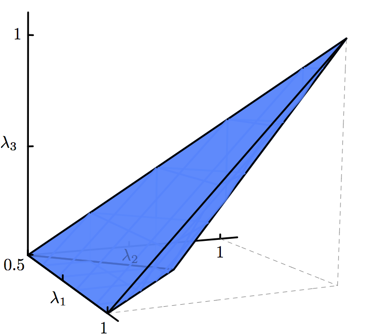
Figure 3.1: Borland–Dennis polytope. The solution of the one-body $n$-representability problem for three fermions with local dimension six, as given by the Borland–Dennis inequalities (3.1). The vertex $(1,1,1)$ corresponds to a single Slater determinant.

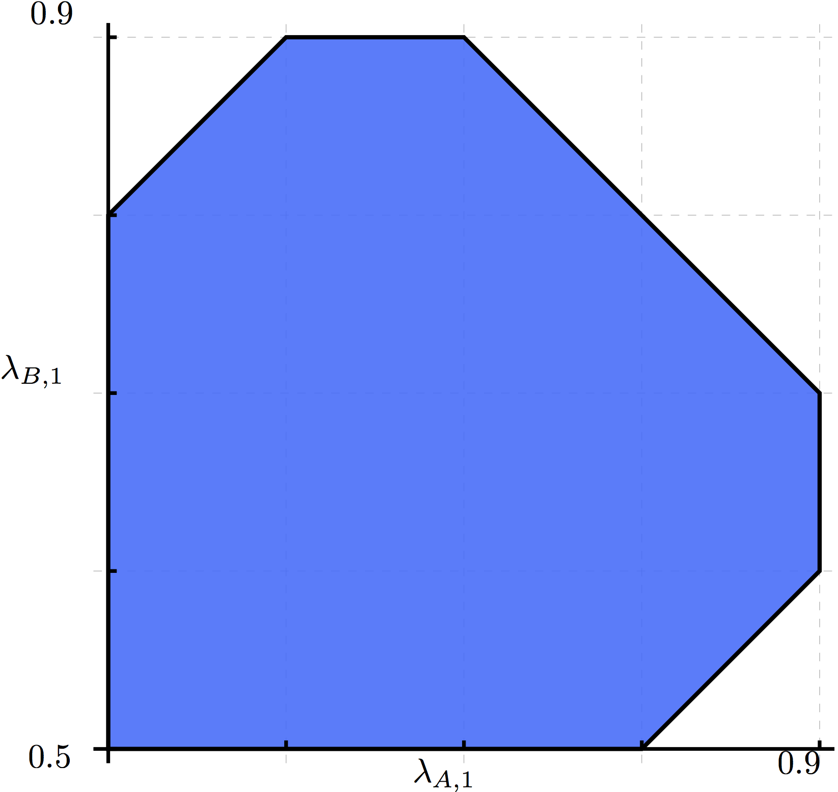
Figure 3.2: Three-qubit polytope. The solution of the one-body quantum marginal problem for pure states of three qubits, as given by the polygonal inequalities (3.2) for $n=3$.

Figure 3.3: Bravyi’s polytope, corresponding to his solution (3.3) of the one-body quantum marginal problem for two qubits and global spectrum $\lambda_{AB}=(0.6,0.3,0.1,0)$.

The connection of the one-body quantum marginal problem to representation theory was first observed in [CM06] by using quantum information methods rather than the theory of Section 2.2 (cf. [CHM07]). Shortly after, a completely general solution was given by Klyachko both for distinguishable particles [Kly04] and for fermions [KA08, Alt08]. Almost simultaneously, Daftuar and Hayden had published a solution to the “one-sided” problem that concerns the constraints between the eigenvalues of $\rho_{AB}$ and $\rho_{A}$ [DH04]. Both results build on previous work by Berenstein and Sjamaar [BS00], who used geometric invariant theory to study the moment polytope for projections of coadjoint orbits; this latter work in turn generalizes techniques from Klyachko’s seminal paper on Weyl’s problem [Kly98] (see the discussion at the end of the preceding chapter). We refer to [Kly04, Knu09] for eloquent expositions of the method. More recently, Ressayre has refined the result of Berenstein and Sjamaar to give an irredundant set of necessary and sufficient inequalities in a very general mathematical setup [Res10b, Res10a]. We remark that a variant of the quantum marginal problem for Gaussian states has been considered in [EG08] (mathematically, this scenario is covered by a more general convexity theorem for non-compact manifolds with proper moment maps).

3.1 Summary of Results

Throughout this chapter we will assume for simplicity that the moment polytope $\Delta_{K}:=\Delta_{K}(\mathbbm{P}(\mathcal{H}))$ is of maximal dimension. For the quantum marginal problem, this assumption is usually satisfied except for two distinguishable particles (which we have already solved in Chapter 2) and in the fermionic Borland–Dennis scenario $\bigwedge^{3}\mathbbm{C}^{6}$ (see (3.1) above), and it is easily checked in practice. Since the moment polytope is a convex polytope, it can be defined by a finite list of linear inequalities

$$\Delta_{K}=\{\lambda\in i\mathfrak{t}^{*}:(\lambda,H_{1})\geq c_{1},\dots,(\lambda,H_{f})\geq c_{f}\},$$

where $H_{1},\dots,H_{f}$ are the normal vectors of the finitely many facets of $\Delta_{K}$. All our normal vectors will always be pointing inwards. Since the moment polytope is obtained by intersecting $\mu_{K}(\mathbbm{P}(\mathcal{H}))$ with the positive Weyl chamber $i\mathfrak{t}^{*}_{+}$, which is a maximal-dimensional polyhedral cone, some of the facets of $\Delta_{K}$ might be subsets of facets of $i\mathfrak{t}^{*}_{+}$, and we call those the trivial facets of the moment polytope.

Our approach in the following is based on analyzing the non-trivial facets in terms of the local differential geometry of their preimages up to second order. Conceptually, such an analysis should be sufficient since the moment map is locally quadratic.

In Section 3.2 we start by studying the moment map to first order. It is well-known that interior points of non-trivial facets are critical values for $(\mu_{K},H)$, where $H$ is the normal vector of the facet. Indeed, this is equivalent to the selection rule from Section 2.3. We show that as a consequence any non-trivial facet of $\Delta_{K}$ is necessarily contained in a hyperplane spanned by weights of the representation $\mathcal{H}$. This already reduces the problem to a finite set of candidates.

In Section 3.3 we then consider the Hessian of the moment map. If a state is mapped into the interior of a non-trivial facet of the polytope then this implies a positive semidefiniteness of the corresponding Hessian in certain tangent directions. We exploit this fact to obtain another necessary condition that is satisfied by non-trivial facets $(-,H)\geq c$ of the moment polytope. To state it, let $\mathfrak{n}_{-}(H<0)$ denote the direct sum of negative root spaces $\mathfrak{g}_{\alpha}$ with $(\alpha,H)<0$ and $\mathcal{H}(H<c)$ the sum of eigenspaces of $\pi(H)$ with eigenvalue smaller than $c$. Then we show that there necessarily exists an eigenvector $\ket{\psi}\in\mathcal{H}$ of $\pi(H)$ with eigenvalue $c$ such that the map

$$\mathfrak{n}_{-}(H<0)\rightarrow\mathcal{H}(H<c),X\mapsto\pi(X)\ket{\psi}$$

is an isomorphism. Conversely, we prove that any inequality $(-,H)\geq c$ that satisfies the above two necessary conditions is a valid inequality of the moment polytope. We thus obtain a complete description of the moment polytope $\Delta_{K}$ in terms of what we call inequalities of Ressayre type (Section 3.3 and Theorem 3.1).

Our notion of a Ressayre-type inequality is closely related to Ressayre’s notion of a dominant pair, and our approach is inspired by his ideas [Res10b, Res10a]. Our description of the moment polytope is also related to a result by Brion [Bri99], as we explain further below. However, while the more refined results of [Bri99, Res10b, Res10a] are established using high-powered algebraic geometry, we proceed in essence by a straightforward differential-geometric analysis, combined with Theorem 2.1.

In Section 3.4, we illustrate the method with some examples. We remark that, crucially, our description of the moment polytope obtained in Theorem 3.1 can be completely automatized: It is straightforward to determine all inequalities of Ressayre type in a mechanical fashion, and hence also on a computer.

3.2 The Torus Action

We use the same notation and conventions as in Chapter 2. Thus let $G$ be a connected reductive algebraic group, $K\subseteq G$ a maximal compact subgroup, and $\Pi\colon G\rightarrow\operatorname{GL}(\mathcal{H})$ a representation on a Hilbert space $\mathcal{H}$ with a $K$-invariant inner product; we denote the infinitesimal representation by $\pi\colon\mathfrak{g}\rightarrow\mathfrak{gl}(\mathcal{H})$. Our object of interest is the moment polytope $\Delta_{K}:=\Delta_{K}(\mathbbm{P}(\mathcal{H}))$ of the projective space associated with the representation $\mathcal{H}$. As stated above, we assume throughout this chapter that $\Delta_{K}$ is of maximal dimension, i.e., $\dim\Delta_{K}=\dim i\mathfrak{t}^{*}$. This is the case whenever there exists a pure state with finite stabilizer, as follows from (2.14) and the local submersion theorem. The facets of $\Delta_{K}$ are of codimension one in $i\mathfrak{t}^{*}$ and may be identified with the defining linear inequalities $(-,H)\geq c$ of the moment polytope.

Definition .

A facet of the moment polytope is trivial if it is of the form $(-,Z_{\alpha})\geq 0$ for some positive root $\alpha\in R_{G,+}$. Otherwise, the facet is called non-trivial.

Non-trivial facets have also been called “general” in the literature [Bri99]. We record the following straightforward observation:

Lemma .

Any non-trivial facet of $\Delta_{K}$ meets the relative interior $i\mathfrak{t}^{*}_{>0}$ of the positive Weyl chamber.

Proof.

Any facet of $\Delta_{K}$ that does not intersect the relative interior of the positive Weyl chamber is fully contained in

$$i\mathfrak{t}^{*}_{+}\setminus i\mathfrak{t}^{*}_{>0}=\bigcup_{\alpha\in R_{G,+}}\{\xi\in i\mathfrak{t}^{*}:(\xi,Z_{\alpha})=0\},$$

which is a finite arrangement of hyperplanes. Since by assumption the facet is of codimension one, it has to be contained in a single one of these hyperplanes. Thus its normal vector is either $\pm Z_{\alpha}$ for some positive root $\alpha$. If it was $-Z_{\alpha}$ then the moment polytope would be strictly contained in the hyperplane $(-,Z_{\alpha})=0$, and therefore not of maximal dimension, in contradiction with our assumption. We conclude that the facet is of the form $(-,Z_{\alpha})\geq 0$, and therefore trivial. ∎

We now consider the moment map for the action of the maximal torus $T\subseteq K$,

$$\mu_{T}\colon\mathbbm{P}(\mathcal{H})\rightarrow i\mathfrak{t}^{*},\quad(\mu_{T}(\rho),X):=\operatorname{tr}\rho\,\pi(X).$$ (3.4)

For the quantum marginal problem, this amounts to considering diagonal entries rather than eigenvalues. Let $\mathcal{H}=\bigoplus_{\omega\in\Omega}\mathcal{H}_{\omega}$ be the decomposition of $\mathcal{H}$ into weight spaces, and $\rho=\lvert\psi\rangle\langle\psi\rvert$ a pure state with $\ket{\psi}=\sum_{\omega}\psi_{\omega}\ket{\omega}$ decomposed accordingly. Then $\mu_{T}$ has the following concrete description:

$$\mu_{T}(\rho)=\sum_{\omega}\lvert\psi_{\omega}\rvert^{2}\omega$$ (3.5)

(cf. the proof of Theorem 2.1). Observe that $\mu_{T}(\rho)$ is a convex combination of weights. It follows that the “Abelian” moment polytope $\Delta_{T}:=\Delta_{T}(\mathbbm{P}(\mathcal{H}))$ of $\mathbbm{P}(\mathcal{H})$ is precisely equal to the convex hull of the set of weights; it is maximal-dimensional since it contains $\Delta_{K}$. More generally, if $\Omega^{\prime}\subseteq\Omega$ is a subset of weights and $\mathcal{H}_{\Omega^{\prime}}:=\bigoplus_{\omega\in\Omega^{\prime}}\mathcal{H}_{\omega}$ then $\Delta_{T}(\mathbbm{P}(\mathcal{H}_{\Omega^{\prime}}))=\operatorname{conv}\Omega^{\prime}$. For the next lemma recall that a critical point of a smooth map $f\colon M\rightarrow M^{\prime}$ is a point $m\in M$ where the differential $df\big{|}_{m}$ is not surjective; a critical value is the image $f(m)$ of a critical point [Lee13].

Lemma .

The set of critical values of $\mu_{T}$ is equal to the union of the codimension-one convex hulls of subsets of weights.

Proof.

Let $\rho=\lvert\psi\rangle\langle\psi\rvert\in\mathbbm{P}(\mathcal{H})$ with weight decomposition $\ket{\psi}=\sum_{\omega}\psi_{\omega}\ket{\omega}$. By (3.5), $\mu_{T}(\rho)$ is a convex combination of weights in $\Omega_{\rho}:=\{\omega:\psi_{\omega}\neq 0\}$. By (2.13) and non-degeneracy of the symplectic form, $\rho$ is a critical point if and only if there exists $0\neq X\in\mathfrak{t}$ such that $X_{\rho}=[\pi(X),\rho]=0$, i.e., if and only if $(\omega-\omega^{\prime})(X)=0$ for any two $\omega\neq\omega^{\prime}\in\Omega_{\rho}$. It follows that $\rho$ is a critical point if and only if the convex hull of $\Omega_{\rho}$ is of positive codimension.

In particular, any critical value is contained in a convex hull of weights of codimension one, since we may always add additional weights. Conversely, if $\Omega^{\prime}\subseteq\Omega$ is a subset of weights that spans a convex hull of codimension one then $\Delta_{T}(\mathbbm{P}(\mathcal{H}_{\Omega^{\prime}}))=\operatorname{conv}\Omega^{\prime}$ consists of critical values. ∎

We now derive a basic necessary condition that cuts down the defining inequalities of the moment polytope to a finite set of candidates.

Lemma .

Any non-trivial facet of $\Delta_{K}$ is contained in an affine hyperplane spanned by a subset of weights.

Proof.

By Section 3.2, the intersection of any non-trivial facet with the interior of the positive Weyl chamber $i\mathfrak{t}^{*}_{>0}$ is non-empty. Each point in this intersection is a critical value for $(\mu_{K},H)=(\mu_{T},H)$ by selection rule (Section 2.3), hence of $\mu_{T}$, and therefore contained in an affine hyperplane spanned by a subset of weights (Section 3.2). Since this is true for all points in the intersection, which contains the relative interior of the facet, it follows that the facet is in fact contained in a single such hyperplane. ∎

We remark that if $(\vec{a},\vec{b})\in\mathbbm{R}^{a+b}$ is an extremal edge in the sense of [Kly04] and $\vec{c}\in\mathbbm{R}^{ab}$ any vector with components $a_{i}+b_{j}$ then $H:=(\vec{a},\vec{b},-\vec{c})$ is the normal vector of a linear hyperplane spanned by weights of $\mathbbm{C}^{a}\otimes\mathbbm{C}^{b}\otimes\mathbbm{C}^{ab}$. Thus the inequalities produced in [Kly04] for the mixed-state problem satisfy the conclusion of the lemma.

3.3 Facets of the Moment Polytope

Throughout this section, let $\rho$ be the preimage of a point $\mu_{K}(\rho)\in i\mathfrak{t}^{*}_{>0}$ on the facet $(-,H)\geq c$ of the moment polytope. We have seen that the selection rule Section 2.3 shows that $\rho$ is a critical point of the component $(\mu_{K},H)$, and we have used this in Section 3.2 to gain information on the set of possible facets.

The Hessian

It is thus natural to continue by studying the Hessian of $(\mu_{K},H)$, which is a quadratic form $Q(-,-)$ on the tangent space at $\rho$. Since $\rho$ is a critical point, we can compute it by

$$Q(X_{\rho},X_{\rho}) =\partial_{t}^{2}\,(\mu_{K}(e^{Xt}\rho e^{-Xt}),H)\big{|}_{t=0}$$

$$=\partial_{t}^{2}\,\operatorname{tr}\rho\,e^{-Xt}\pi(H)e^{Xt}\big{|}_{t=0}$$

$$=\operatorname{tr}\rho\,\left(X^{2}\pi(H)-2X\pi(H)X+\pi(H)X^{2}\right)$$

$$=\operatorname{tr}\rho\,[[\pi(H),X],X]$$

for all anti-Hermitian operators $X\in\mathfrak{u}(\mathcal{H})$. It follows that [GS84b, (32.8)]

$$Q(X_{\rho},Y_{\rho})=\operatorname{tr}\rho\,[[\pi(H),X],Y]=\omega([\pi(-iH),X]_{\rho},Y_{\rho}).$$ (3.6)

for all $X,Y\in\mathfrak{u}(\mathcal{H})$ (which is indeed symmetric in $X$ and $Y$). We now decompose

$$\mathcal{H}=\mathcal{H}(H<c)\oplus\mathcal{H}(H=c)\oplus\mathcal{H}(H>c),$$ (3.7)

where $\mathcal{H}(H<c)=\bigoplus_{\omega:(\omega,H)<c}\mathcal{H}_{\omega}$ is the sum of the eigenspaces of the Hermitian operator $\pi(H)$ with eigenvalue less than $c$, etc. Then we have the following interpretation of the index of the Hessian (the dimension of a maximal subspace on which the quadratic form $Q$ is negative definite):

Lemma .

The index of the Hessian at $\rho$ is equal to the real dimension of $\mathcal{H}(H<c)$.

Proof.

Recall from (2.8) that the tangent space at $\rho=\lvert\psi\rangle\langle\psi\rvert$ can be identified with the orthogonal complement of $\ket{\psi}$ in $\mathcal{H}$. For any $\ket{\phi}\in\ket{\psi}^{\perp}$, the corresponding tangent vector is $V=\lvert\phi\rangle\langle\psi\rvert+\lvert\psi\rangle\langle\phi\rvert\in T_{\rho}\mathbbm{P}(\mathcal{H})$, which we can write as $X_{\rho}=[X,\rho]$ for $X=\lvert\phi\rangle\langle\psi\rvert-\lvert\psi\rangle\langle\phi\rvert\in\mathfrak{u}(\mathcal{H})$. By (3.6),

$$Q(V,V) =Q(X_{\rho},X_{\rho})=\operatorname{tr}\rho\,[[\pi(H),X],X]=\operatorname{tr}X_{\rho}\,[\pi(H),X]$$

$$=2\left(\braket{\phi}{\pi(H)}{\phi}-\braket{\phi}{\phi}\braket{\psi}{\pi(H)}{\psi}\right)$$

$$=2\left(\braket{\phi}{\pi(H)}{\phi}-\braket{\phi}{\phi}(\mu_{K}(\rho),H)\right)$$

$$=2\braket{\phi}{\pi(H)-c}{\phi}.$$

Since $\psi$ itself is in $\mathcal{H}(H=c)$ by the selection rule, the claim follows. ∎

Since $(\mu_{K}(\rho),H)=c$ and $d(\mu_{K},H)\big{|}_{\rho}=0$, the Hessian is necessarily positive semidefinite on the subspace of those tangent vectors that get mapped to $i\mathfrak{t}^{*}$. Indeed, let $V\in d\mu_{K}^{-1}\big{|}_{\rho}(i\mathfrak{t}^{*})$ and consider the curve $\rho_{t}$ from Section 2.3. Then,

$$(\mu_{K}(\rho_{t}),H)=c+\frac{t^{2}}{2}Q(V,V)+O(t^{3}),$$ (3.8)

which shows that, indeed, $Q(V,V)\geq 0$. The subspace of all such $V$ can be computed in a different way. For this, let $\mathfrak{r}=\bigoplus_{\alpha\in R_{G,+}}\mathfrak{k}_{\alpha}$ denote the sum of the root spaces of the compact Lie algebra as in (2.5) and

$$M:=\{R_{\rho}=[\pi(R),\rho]:R\in\mathfrak{r}\}\subseteq T_{\rho}\mathbbm{P}(\mathcal{H})$$

the corresponding subspace of tangent vectors. Then,

$$\{V\in T_{\rho}\mathbbm{P}(\mathcal{H}):d\mu_{K}(V)\in i\mathfrak{t}^{*}\}$$

$$= \{V\in T_{\rho}\mathbbm{P}(\mathcal{H}):d(\mu_{K},iR)(V)=0\quad(\forall R\in\mathfrak{r})\}$$

$$= \{V\in T_{\rho}\mathbbm{P}(\mathcal{H}):\omega(V,R_{\rho})=0\quad(\forall R\in\mathfrak{r})\}$$

which is by definition equal to the symplectic complement $M^{\omega}$ of $M$ in $T_{\rho}\mathbbm{P}(\mathcal{H})$. We summarize our discussion in the following lemma.

Lemma .

The Hessian at $\rho$ is positive semidefinite on the subspace

$$M^{\omega}:= \{V\in T_{\rho}\mathbbm{P}(\mathcal{H}):\omega(V,W)=0\quad(\forall W\in M)\}$$ (3.9)

$$= \{V\in T_{\rho}\mathbbm{P}(\mathcal{H}):d\mu_{K}(V)\in i\mathfrak{t}^{*}\}$$

Lemma .

For any $\lambda\in i\mathfrak{t}^{*}_{>0}$, the coadjoint action $\mathfrak{r}\rightarrow i\mathfrak{k}^{*}$, $R\mapsto\operatorname{ad}^{*}(R)\lambda$ is injective. Therefore, the tangent map $\mathfrak{r}\rightarrow T_{\rho}\mathbbm{P}(\mathcal{H})$, $R\mapsto R_{\rho}$ is injective.

Proof.

The first claim is a reformulation of the fact that the $K$-stabilizer of any $\lambda\in i\mathfrak{t}^{*}_{>0}$ is $T$, while $\mathfrak{k}=\mathfrak{t}\oplus\mathfrak{r}$. The second claim follows from the first, since $\mu_{K}(\rho)\in i\mathfrak{t}^{*}_{>0}$ and $d\mu_{K}(R_{\rho})=\operatorname{ad}^{*}(R)\mu_{K}(\rho)$ by equivariance of the moment map. ∎

Lemma .

The tangent space at $\rho$ decomposes as a direct sum

$$T_{\rho}\mathbbm{P}(\mathcal{H})=M\oplus M^{\omega}$$

and the Hessian $Q$ is block-diagonal with respect to this decomposition.

Proof.

For the first claim we only need to show that $M\cap M^{\omega}=0$, which is standard (see, e.g., [GS82a, Lemma 6.7]): Let $R\in\mathfrak{r}$. Suppose that $R_{\rho}\in M^{\omega}$. That is,

$$\operatorname{ad}^{*}(R)\mu_{K}(\rho)=d\mu_{K}(R_{\rho})\in i\mathfrak{t}^{*}$$

according to (3.9) and equivariance of the moment map. But $[\mathfrak{r},i\mathfrak{t}]\subseteq i\mathfrak{r}$, so it follows that $\operatorname{ad}^{*}(R)\mu_{K}(\rho)=0$ and so $R=0$ and $R_{\rho}=0$, since we have just seen that the coadjoint action of $\mathfrak{r}$ is injective at $\lambda=\mu_{K}(\rho)\in i\mathfrak{t}^{*}_{>0}$ (Section 3.3). Thus $M\cap M^{\omega}=0$ and $M\oplus M^{\omega}=T_{\rho}\mathbbm{P}(\mathcal{H})$ by dimension counting.

For the second claim, observe that (3.6) immediately implies that

$$Q(R_{\rho},V)=\omega([\pi(-iH),\pi(R)]_{\rho},V)=\omega([-iH,R]_{\rho},V)=0$$

for all $R_{\rho}\in M$ and $V\in M^{\omega}$, since $[-iH,R]\in\mathfrak{r}$ and hence $[-iH,R]_{\rho}\in M$. ∎

Lemma .

The index of the Hessian at $\rho$ is equal to twice the number of positive roots $\alpha\in R_{G,+}$ such that $(\alpha,H)>0$.

Proof.

Since $Q$ is positive semidefinite on $M^{\omega}$ (Section 3.3) and block-diagonal with respect to the decomposition $T_{\rho}\mathbbm{P}(\mathcal{H})=M\oplus M^{\omega}$ (Section 3.3), it suffices to compute the index of $Q$ on $M=\{R_{\rho}:R\in\mathfrak{r}\}$. By (3.6),

$$Q(R_{\rho},S_{\rho})=\operatorname{tr}\rho[[\pi(H),\pi(R)],\pi(S)]=(\mu_{K}(\rho),[[H,R],S]).$$

Since the tangent map $R\mapsto R_{\rho}$ is injective (Section 3.3), we may instead consider the form

$$\widetilde{Q}(R,S):=(\mu_{K}(\rho),[[H,R],S])$$

on $\mathfrak{r}$. For this, observe that $\widetilde{Q}$ is block-diagonal with respect to $\mathfrak{r}=\bigoplus_{\alpha\in R_{G,+}}\mathfrak{k}_{\alpha}$, since for all $R\in\mathfrak{k}_{\alpha}$ and $S\in\mathfrak{k}_{\beta}$, $[[H,R],S]\in i\mathfrak{k}_{\alpha\pm\beta}$, while $\mu_{K}(\rho)\in i\mathfrak{t}^{*}$. And for each root space $\mathfrak{k}_{\alpha}$, we have that

$$\widetilde{Q}(iX_{\alpha},iX_{\alpha})=-(\mu_{K}(\rho),[[H,X_{\alpha}],X_{\alpha}])$$

$$= -i(\alpha,H)(\mu_{K}(\rho),[Y_{\alpha},X_{\alpha}])=-2(\alpha,H)(\mu_{K}(\rho),Z_{\alpha})$$

where we have used the “Pauli matrices” $X_{\alpha},Y_{\alpha},Z_{\alpha}$ and their commutation relations (2.6). Likewise, $\widetilde{Q}(iY_{\alpha},iY_{\alpha})=-2(\alpha,H)(\mu_{K}(\rho),Z_{\alpha})$, while $\widetilde{Q}(iX_{\alpha},iY_{\alpha})=0$. Since $(\mu_{K}(\rho),Z_{\alpha})>0$, we conclude that the index of $Q$ is equal to twice the number of positive roots $\alpha$ with $(\alpha,H)>0$. ∎

Ressayre Elements

So far we have used the Lie algebra $\mathfrak{k}$ of the compact Lie group in our analysis. We will now translate the preceding to the complexified setting. To this end, we consider the Lie algebra $\mathfrak{n}_{-}=\bigoplus_{\alpha\in R_{G,-}}\mathfrak{g}_{\alpha}$ of the negative unipotent subgroup, which plays a role analogous to $\mathfrak{r}$ for states $\rho$ that are mapped into the positive Weyl chamber (compare the following with Section 3.3).

Lemma .

The tangent map $\mathfrak{n}_{-}\rightarrow\mathcal{H},X\to\pi(X)\ket{\psi}$ is injective.

Proof.

Let $E_{-}:=\sum_{\alpha\in R_{G,+}}z_{\alpha}E_{-\alpha}$ be an arbitrary element in $\mathfrak{n}_{-}$. Since $\pi(E_{\pm\alpha})^{\dagger}=\pi(E_{\mp\alpha})$, we find that $\pi(E_{-})^{\dagger}=\pi(E_{+})$ with $E_{+}:=\sum_{\alpha\in R_{G,+}}\bar{z}_{\alpha}E_{\alpha}$ (the Cartan involution of $E_{-}$). Therefore,

$$\lVert\pi(E_{-})\ket{\psi}\rVert^{2}= \operatorname{tr}\rho\,\pi(E_{+})\pi(E_{-})=\operatorname{tr}\rho\,\pi([E_{+},E_{-}])+\lVert\pi(E_{+})\ket{\psi}\rVert^{2}$$

$$\geq \operatorname{tr}\rho\,\pi([E_{+},E_{-}]).$$

But (2.4) and (2.6) imply that

$$[E_{+},E_{-}]-\sum_{\alpha\in R_{G,+}}\lvert z_{\alpha}\rvert^{2}Z_{\alpha}\in i\mathfrak{r},$$

so that by using $\mu_{K}(\rho)\in i\mathfrak{t}^{*}_{>0}$ we find that

$$\operatorname{tr}\rho\,\pi([E_{+},E_{-}])=\sum_{\alpha\in R_{G,+}}\lvert z_{\alpha}\rvert^{2}(\mu_{K}(\rho),Z_{\alpha})>0.\qed$$

In contrast to Section 3.3, which continues to hold true if $\mu_{K}(\rho)$ is mapped to the relative interior of a different Weyl chamber (since $K$ is invariant under the Weyl group), it is important in Section 3.3 to choose the negative unipotent subgroup (relative to the choice of positive Weyl chamber). For example, consider an irreducible $G$-representation $\mathcal{H}=V_{G,\lambda}$ with highest weight $\lambda\in i\mathfrak{t}^{*}_{>0}$ and highest weight vector $\ket{\lambda}$. Then $\mu_{K}(\lvert\lambda\rangle\langle\lambda\rvert)=\lambda\in i\mathfrak{t}^{*}_{>0}$ by Section 2.2, and the “lowering operators” in $\mathfrak{n}_{-}$ act indeed injectively (all $\pi(E_{-\alpha})\ket{\lambda}$ live in different weight spaces and are non-zero, since $\pi(E_{\alpha})\pi(E_{-\alpha})\ket{\lambda}=\pi(Z_{\alpha})\ket{\lambda}=(\lambda,Z_{\alpha})\ket{\lambda}\neq 0$). On the other hand, the “raising operators” in the positive nilpotent Lie algebra $\mathfrak{n}_{+}$ annihilate the highest weight vector (by definition).

We now decompose the Lie algebra $\mathfrak{n}_{-}$ similarly to (3.7),

$$\mathfrak{n}_{-}=\mathfrak{n}_{-}(H<0)\oplus\mathfrak{n}_{-}(H=0)\oplus\mathfrak{n}_{-}(H>0),$$

where $\mathfrak{n}_{-}(H<0)=\bigoplus_{\alpha\in R_{G,-}:(\alpha,H)<0}\mathfrak{g}_{\alpha}$ is the sum of the complex root spaces with negative $H$-weight $(\alpha,H)<0$, etc. By combining Lemmas 3.3 and 3.3 and using $R_{G,-}=-R_{G,+}$, we observe that

$$\dim_{\mathbbm{C}}\mathcal{H}(H<c)=\dim_{\mathbbm{C}}\mathfrak{n}_{-}(H<0).$$ (3.10)

Note that $\pi(\mathfrak{n}_{-}(H<0))\mathcal{H}(H=c)\subseteq\mathcal{H}(H<c)$, since for any $\ket{\psi}\in\mathcal{H}(H=c)$ and $X\in\mathfrak{g}_{\alpha}$ we have that

$$\pi(H)\pi(X)\ket{\psi}=\pi([H,X])\ket{\psi}+\pi(X)\pi(H)\ket{\psi}=((\alpha,H)+c)\pi(X)\ket{\psi}.$$

Thus we obtain the following important result:

Proposition .

Let $\rho=\lvert\psi\rangle\langle\psi\rvert\in\mathbbm{P}(\mathcal{H})$ such that $\mu_{K}(\rho)\in i\mathfrak{t}^{*}_{>0}$ is a point on the facet of the moment polytope corresponding to the inequality $(-,H)\geq c$. Then $\ket{\psi}\in\mathcal{H}(H=c)$ and the tangent map restricts to an isomorphism

$$\mathfrak{n}_{-}(H<0)\rightarrow\mathcal{H}(H<c),\quad X\mapsto\pi(X)\ket{\psi}.$$

Proof.

The fact that $\ket{\psi}\in\mathcal{H}(H=c)$ is just a reformulation of the selection rule. By the preceding discussion, the tangent map is well-defined as a map from $\mathfrak{n}_{-}(H<0)$ to $\mathcal{H}(H<c)$; it is injective by Section 3.3 and surjective since the dimensions agree according to (3.10). ∎

We now prove a partial converse to Section 3.3. Our proof is inspired by the argument of Ressayre [Res10b].

Proposition .

Suppose there exists $\ket{\psi}\in\mathcal{H}(H=c)$ such that the tangent map

$$\mathfrak{n}_{-}(H<0)\rightarrow\mathcal{H}(H<c),\quad X\mapsto\pi(X)\ket{\psi}.$$

is surjective. Then $(-,H)\geq c$ is a valid inequality for the moment polytope.

Proof.

Consider the smooth map

$$N_{-}\times\mathcal{H}(H\geq c)\rightarrow\mathcal{H},\quad(g,\ket{\phi})\mapsto\Pi(g)\ket{\phi}.$$

Its differential at $(1,\ket{\psi})$ is the linear map

$$\mathfrak{n}_{-}\oplus\mathcal{H}(H\geq c)\rightarrow\mathcal{H},\quad(X,\ket{\phi})\mapsto\pi(X)\ket{\psi}+\ket{\phi}.$$

The assumption implies that this map is surjective. It follows that $\Pi(N_{-})\mathcal{H}(H\geq c)\subseteq\mathcal{H}$ contains a small Euclidean ball around $\ket{\psi}$. In particular, any polynomial that is zero on $\Pi(N_{-})\mathcal{H}(H\geq c)$ is zero everywhere on $\mathcal{H}$.

We now prove the inequality. By the description of the moment polytope of Theorem 2.1, it suffices to show that $(\lambda/k,H)\geq c$ for all highest weights $\lambda$ such that $V^{*}_{G,\lambda}\subseteq R_{k}(\mathcal{H})$. Recall that the highest weight of $V^{*}_{G,\lambda}$ is $\lambda^{*}=-w_{0}\lambda$, where $w_{0}$ is the longest Weyl group element that flips the positive and negative roots. Consider a lowest weight vector, i.e., a homogeneous polynomial $P\in R_{k}(\mathcal{H})$ that is a weight vector of weight $-\lambda$ and stabilized by $N_{-}$. Then $\pi(H)P=-(\lambda,H)P$ and the restriction of $P$ to $\mathcal{H}(H\geq c)$ is non-zero by our discussion above. But this restriction is an element of $R_{k}(\mathcal{H}(H\geq c))=\operatorname{Sym}^{k}(\mathcal{H}(H\geq c))^{*}$, the space of homogeneous polynomials of degree $k$ on $\mathcal{H}(H\geq c)$. Thus all $H$-weights in $R_{k}(\mathcal{H}(H\geq c))$ are less or equal to $-kc$. It follows that $-(\lambda,H)\leq-kc$, hence $(\lambda/k,H)\geq c$, as we set out to prove. ∎

We remark that Section 3.3 holds unconditionally without any assumption on the dimension of the moment polytope $\Delta_{K}$. We summarize our findings in the following definition and theorem:

Definition .

An inequality $(-,H)\geq c$ is said to be of Ressayre type if

1. $(-,H)=c$ is an affine hyperplane spanned by a subset of weights.

2. There exists $\ket{\psi}\in\mathcal{H}(H=c)$ such that the map

   $$\mathfrak{n}_{-}(H<0)\rightarrow\mathcal{H}(H<c),\quad X\mapsto\pi(X)\ket{\psi}$$

   is an isomorphism.

We note that the first condition is invariant under the action of the Weyl group.

Theorem 3.1.

The moment polytope is given by

$$\Delta_{K}=\{\lambda\in\mathfrak{t}^{*}_{+}:(\lambda,H)\geq c\text{ for all Ressayre-type inequalities}\}.$$

Proof.

This follows directly from Section 3.2, Section 3.3 and Section 3.3. ∎

Theorem 3.1 gives a complete description of the moment polytope of the projective space of an arbitrary $G$-representation $\mathcal{H}$ (under the assumption that $\Delta_{K}$ is of maximal dimension). The set of inequalities thus obtained may still be redundant (i.e., not all inequalities necessarily correspond to facets of the moment polytope). In contrast, Ressayre’s well-covering pairs [Res10b, Res10a] characterize the facets of the moment polytope precisely. Our characterization is also related to [Bri99, Theorem 2], which uses algebraic geometry to characterize non-trivial faces of arbitrary codimension. Unlike Section 3.3, it relies on an assumption about lower-dimensional moment polytopes, which can in principle be obtained recursively.

It is straightforward to enumerate all inequalities of Ressayre type. Since there are only finitely many weights, the first condition in Section 3.3 cuts down the number of possible inequalities down to a finite list of candidates, and for each such candidate $(-,H)\geq c$, the second condition can be easily checked: Indeed, we only need to verify that $\dim\mathfrak{n}_{-}(H<0)=\dim\mathcal{H}(H<c)$ and that the determinant polynomial

$$\mathcal{H}(H=c)\rightarrow\mathbbm{C},\ket{\psi}\mapsto\det\Big{(}\mathfrak{n}_{-}(H<0)\ni X\mapsto\pi(X)\ket{\psi}\in\mathcal{H}(H<c)\Big{)}$$ (3.11)

is non-zero (take the determinant with respect to any fixed pair of bases). Both steps can easily be implemented in a short computer program.

We remark that in view of Theorem 2.1 the non-vanishing of the determinant (3.11) can be understood as a statement about a moment polytope of $\mathbbm{P}(\mathcal{H}(H=c))$. In this way, further necessary conditions can be extracted that cut down the list of candidate inequalities. We will comment on this aspect and related results in a forthcoming paper.

3.4 Examples

We now illustrate the method by considering some of the examples discussed at the beginning of the chapter.

Qubits

We will start by showing that the solution of the one-body quantum marginal problem for $n$ qubits is indeed given by the polygonal inequalities (3.2), which we recall are given by

$$\lambda_{1,1}+\dots+\lambda_{n-1,1}\leq(n-2)+\lambda_{n,1},$$ (3.12)

and its permutations.

Let $K=\operatorname{SU}(2)^{\times n}$, $G=\operatorname{SL}(2)^{\times n}$ its complexification, and $\pi\colon\mathfrak{g}\rightarrow\mathfrak{gl}(\mathcal{H})$ the infinitesimal representation of the Lie algebra on $\mathcal{H}=(\mathbbm{C}^{2})^{\otimes n}$, the Hilbert space of $n$ qubits. The Lie algebra $i\mathfrak{t}$ is spanned by the Pauli $\sigma_{z}$-matrices $Z_{1},\dots,Z_{n}$ of the individual $\mathfrak{sl}(2)$ summands, and each $Z_{k}$ acts on the respective factor of the Hilbert space by the Pauli $\sigma_{z}$-matrix $\left(\begin{smallmatrix}1&\\ &-1\end{smallmatrix}\right)$. Likewise, there are $n$ positive roots $\alpha_{1},\dots,\alpha_{n}$ and they satisfy $(\alpha_{k},Z_{l})=2\delta_{kl}$.

By using that $\lambda_{k,1}+\lambda_{k,2}=1$ for each qubit, we find that (3.12) is equivalent to the following inequality for the moment polytope $\Delta_{K}$,

$$(-,\underbrace{-Z_{1}-\dots-Z_{n-1}+Z_{n}}_{=:H})\geq 2-n,$$

which we will now prove by using the criterion of Section 3.3.

For this, let $\ket{0}$ and $\ket{1}$ denote the standard basis vectors of $\mathbbm{C}^{2}$ and $\ket{\vec{x}}$ the corresponding product basis vectors of $\mathcal{H}$, where $\vec{x}\in\{0,1\}^{\times n}$. Then $\pi(Z_{k})\ket{\vec{x}}=(1-2x_{k})\ket{\vec{x}}$, so that each basis vector $\ket{\vec{x}}$ is a weight vector whose weight is given by $(\omega,Z_{k})=(1-2x_{k})$ for all $k=1,\dots,n$. In particular, the eigenvalue of $\pi(H)$ is $(\omega,H)=2-n+2(x_{1}+\dots+x_{n-1}-x_{n})$, so that

$$\mathcal{H}(H=2-n) =\operatorname{span}_{\mathbbm{C}}\{\ket{\vec{x}}:x_{1}+\dots+x_{n-1}-x_{n}=0\}$$

$$=\operatorname{span}_{\mathbbm{C}}\{\ket{10\dots 01},\dots,\ket{0\dots 011},\ket{0\dots 0}\}$$ (3.13)

$$\mathcal{H}(H<2-n) =\mathbbm{C}\ket{0\dots 01}.$$

On the other hand, there is precisely one negative root with $(-,H)<0$, namely $-\alpha_{n}$. Therefore,

$$\mathfrak{n}_{-}(H<0)=\mathfrak{g}_{-\alpha_{n}}=\mathbbm{C}E_{-n},$$

where the generator $E_{-n}$ acts as the “lowering operator” $\lvert 1\rangle\langle 0\rvert$ on the $n$-th tensor factor of $\mathcal{H}$. But then $\pi(E_{-n})\ket{0\dots 0}=\ket{0\dots 01}$, so that the map

$$\mathfrak{n}_{-}(H<0)\rightarrow\mathcal{H}(H<2-n),\quad X\mapsto\pi(X)\ket{\psi}$$

is indeed an isomorphism for $\ket{\psi}=\ket{0\dots 0}\in\mathcal{H}(H=2-n)$. Thus Section 3.3 shows that the polygonal inequality (3.12) is indeed valid. We remark that the $n$ weights corresponding to (3.13) span the hyperplane $(-,H)=2-n$ and hence the inequality is of Ressayre type—but we did not need this to apply the proposition. The other polygonal inequalities follow from the above since the solution to the one-body quantum marginal problem is symmetric under permutation of the qubits.

To see that there are no further constraints, we could now verify that the polygonal inequalities imply all other Ressayre-type inequalities (which, according to Theorem 3.1, characterize the moment polytope completely). In the case at hand, we observe instead that for each $k\leq n-2$ as well as for $k=n$ the quantum states

$$\ket{0}^{\otimes k}\otimes\left(\ket{0}^{\otimes n-k}+\ket{1}^{\otimes n-k}\right)/\sqrt{2}$$

have local eigenvalues

$$\lambda_{1,1}=\dots=\lambda_{k,1}=1,\quad\lambda_{k+1,1}=\dots=\lambda_{n,1}=0.5,$$

and likewise for their permutations. These points are just the vertices of the convex polytope cut out by the polygonal inequalities (3.2), which is therefore equal to the moment polytope.

This idea of producing an inner approximation from the local eigenvalues of suitably constructed quantum states – or from the normalized highest weights $\lambda/k$ of concretely exhibited representations $V_{G,\lambda}^{*}\subseteq R_{k}(\mathbbm{X})$ [KA08, Alt08] – and then comparing with an outer approximation defined by a subset of valid inequalities (obtained, e.g., from Section 3.3) is rather useful to compute moment polytopes in practice.

Mixed States of Two Qubits

We now consider the mixed-state one-body quantum marginal problem for two qubits. We will focus on the last constraint in (3.3),

$$\lvert\lambda_{A,1}-\lambda_{B,1}\rvert\leq\min\{\lambda_{AB,1}-\lambda_{AB,3},\lambda_{AB,2}-\lambda_{AB,4}\},$$

which by symmetry can be reduced to the following two linear inequalities

$$\lambda_{A,1}-\lambda_{B,1} \leq\lambda_{AB,1}-\lambda_{AB,3},$$ (3.14)

$$\lambda_{A,1}-\lambda_{B,1} \leq\lambda_{AB,2}-\lambda_{AB,4}.$$

In [Bra04], the inequalities are proved by a “formidable” two-page calculation that is tailored towards the two-qubit scenario. In contrast we will obtain (3.14) completely mechanically by using the general machinery developed in Section 3.3.

For this, we consider its equivalent formulation in terms of pure states on $\mathcal{H}=\mathbbm{C}^{2}\otimes\mathbbm{C}^{2}\otimes\mathbbm{C}^{4}$. Let $K=\operatorname{SU}(2)\times\operatorname{SU}(2)\times\operatorname{SU}(4)$ and $G=\operatorname{SL}(2)\times\operatorname{SL}(2)\times\operatorname{SL}(4)$. The roots are the union of the roots of the individual factors, and we will denote them by $\alpha_{A,ij}$, $\alpha_{B,ij}$ and $\alpha_{C,ij}$ according to the notation and conventions in Table 2.1. Thus a root is positive if $i<j$ and negative if $i>j$. We write $E_{A,ij}$, etc., for the generators of the root spaces $\mathfrak{g}_{\alpha_{A,ij}}$; they act “raising and lowering operators” $\lvert i\rangle\langle j\rvert$ on the respective tensor factor. Similarly, the corresponding generators of $i\mathfrak{t}$ are denoted by $Z_{A,ij}$, etc.; they act as the diagonal matrices $\lvert i\rangle\langle i\rvert-\lvert j\rangle\langle j\rvert$ on the respective tensor factor of the Hilbert space. Using these definitions, the first inequality in (3.14) can be written as the following linear inequality for the moment polytope $\Delta_{K}$:

$$(\lambda,\underbrace{-Z_{A,12}+Z_{B,12}+2Z_{C,13}}_{=:H})\geq 0$$

Finally, let $\ket{ijk}$ denote the standard product basis vectors of $\mathcal{H}=\mathbbm{C}^{2}\otimes\mathbbm{C}^{2}\otimes\mathbbm{C}^{4}$ ($i,j=1,2$, $k=1,\dots,4$). Then,

$$\mathcal{H}(H=0) =\operatorname{span}_{\mathbbm{C}}\{\ket{112},\ket{114},\ket{121},\ket{213},\ket{222},\ket{224}\},$$

$$\mathcal{H}(H<0) =\operatorname{span}_{\mathbbm{C}}\{\ket{113},\ket{122},\ket{124},\ket{223},\ket{123}\},$$ (3.15)

while

$$\mathfrak{n}_{-}(H<0)=\operatorname{span}_{\mathbbm{C}}\{E_{B,21},E_{C,21},E_{C,41},E_{C,32},E_{C,31}\}.$$ (3.16)

It remains to verify that the map

$$\mathfrak{n}_{-}(H<0)\rightarrow\mathfrak{\mathcal{H}}(H<0),X\mapsto\pi(X)\ket{\psi}$$ (3.17)

is an isomorphism for some $\ket{\psi}\in\mathcal{H}(H=0)$. We can do so completely mechanically by computing the determinant polynomial (3.11) with respect to the bases in (3.15) and (3.16). Using that each $E_{X,ij}$ acts by $\lvert i\rangle\langle j\rvert$ on the corresponding tensor factor, we readily find that it is given by

$$\det\begin{pmatrix}0&0&0&\psi_{112}&0\\ \psi_{112}&\psi_{121}&0&0&0\\ \psi_{114}&0&\psi_{121}&0&0\\ \psi_{213}&0&0&\psi_{222}&0\\ 0&0&0&0&\psi_{121}\end{pmatrix}=-\psi_{121}^{3}\psi_{112}\psi_{213}\neq 0$$

and thus is indeed non-zero. For example, $\ket{\psi}=\ket{121}+\ket{112}+\ket{213}\in\mathcal{H}(H=0)$ is a choice for which (3.17) is an isomorphism. Thus Section 3.3 shows that the first inequality in (3.14) is indeed a valid inequality for the one-body marginal problem for mixed states of two qubits. The second inequality can be established in a completely identical fashion.

Three Qutrits

For our next example, we consider the one-body quantum marginal problem for pure states of three qubits, $\mathcal{H}=\mathbbm{C}^{3}\otimes\mathbbm{C}^{3}\otimes\mathbbm{C}^{3}$. We will focus on the inequality

$$(\lambda_{A,1}+2\lambda_{A,2})+(2\lambda_{B,1}+\lambda_{B,2})-(4\lambda_{C,1}+3\lambda_{C,2}+2\lambda_{C,3})\leq 0$$ (3.18)

corresponding to the facet $h_{7}$ in [Fra02, Proposition 5.1].

The significance of this facet is that it is neither trivial nor does it contain the vertex $\lambda_{A,1}=\lambda_{B,1}=\lambda_{C,1}=1$ of the moment polytope that corresponds to product states $\ket{000}$ – unlike in the case of $n$ qubits, where the polygonal inequalities (3.2) are saturated for product states (cf. Figure 3.3). As was pointed out in [Fra02, Remark 5.3], this shows that in general the moment polytope is not determined by the trivial facets together with the local cone at the point corresponding to the product state (more generally, the local cone at the highest weight of an irreducible representation).

Let $K=\operatorname{SU}(3)\times\operatorname{SU}(3)\times\operatorname{SU}(3)$ and $G=\operatorname{SL}(3)\times\operatorname{SL}(3)\times\operatorname{SL}(3)$ with their tensor product action on the Hilbert space $\mathcal{H}$. Using the same notation as in the preceding example, we find that (3.18) can be written in the form

$$(\lambda,\underbrace{-Z_{A,23}-Z_{B,13}+Z_{C,13}}_{=:H})\geq-1.$$

It can be readily computed that

$$\mathcal{H}(H=-1) =\operatorname{span}_{\mathbbm{C}}\{\ket{112},\ket{123},\ket{211},\ket{222},\ket{233},\ket{313}\},$$

$$\mathcal{H}(H<-1) =\operatorname{span}_{\mathbbm{C}}\{\ket{113},\ket{212},\ket{213},\ket{223}\},$$

$$\mathfrak{n}_{-}(H<0) =\operatorname{span}_{\mathbbm{C}}\{E_{A,21},E_{C,21},E_{C,31},E_{C,32}\}.$$

The determinant polynomial is

$$\det\begin{pmatrix}0&0&0&\psi_{112}\\ \psi_{112}&\psi_{211}&0&0\\ 0&0&\psi_{211}&0\\ \psi_{123}&0&0&\psi_{222}\end{pmatrix}=-\psi_{112}\psi_{123}\psi_{211}^{2}\neq 0$$

and thus (3.18) is indeed a valid inequality.

Three Fermions with Total Spin $1/2$

Our last example is motivated by quantum chemistry. We consider three fermions with $d$-dimensional orbital degree of freedom and spin $1/2$, as described by the Hilbert space $\bigwedge^{3}(\mathbbm{C}^{d}\otimes\mathbbm{C}^{2})$ [KA08, §3.1]. Let $G=\operatorname{SL}(d)\times\operatorname{SL}(2)$ and $K=\operatorname{SU}(d)\times\operatorname{SU}(2)$. Then the moment map sends a pure state $\rho$ of three fermions to the pair $(\gamma_{O},\gamma_{S})$, where $\gamma_{O}$ is the first-order density matrix of the orbital degrees of freedom and $\gamma_{S}$ likewise for the spin. Thus the moment polytope encodes the constraints between the orbital occupation numbers and spin occupation numbers. The anti-symmetric subspace is not an irreducible $G$-representation but rather decomposes as follows:

$$\bigwedge^{3}(\mathbbm{C}^{d}\otimes\mathbbm{C}^{2})= V^{d}_{\yng(2,1)}\otimes V^{2}_{\yng(2,1)}\;\oplus\;V^{d}_{\yng(1,1,1)}\otimes V^{2}_{\yng(3)}$$

(In analogy to (2.25), each Young diagram is paired with its transpose.) The different summands in the decomposition correspond to different sectors of total spin $J=1/2,3/2$. Now suppose that we know in addition that the global state is a pure state in the sector for total spin $J=1/2$:

$$\mathcal{H}=V^{d}_{\yng(2,1)}\otimes V^{2}_{\yng(2,1)}\cong V^{d}_{\yng(2,1)}\otimes\mathbbm{C}^{2}.$$

Then the problem of determining the relation between the orbital and spin occupation numbers amounts to computing the moment polytope for the $G$-representation $\mathcal{H}$. This illustrates how representations other than those in Table 2.3 may enter the picture due to physical considerations. In [KA08, §6.1] it was observed that there are five inequalities which are “apparently independent” of the orbital dimension $d$, as they verified for $d=4,5$. Their first equation is

$$\lambda_{1}-\lambda_{2}\leq 1+\mu_{2}$$ (3.19)

where $\lambda_{1}\geq\dots\geq\lambda_{d}$ denote the natural occupation numbers of the first-order orbital density matrix $\gamma_{O}$, normalized to trace $3$, and $\mu_{1}\geq\mu_{2}$ the eigenvalues of the spin density matrix $\rho_{S}=\gamma_{S}/3$, normalized to trace $1$.

We will now prove (3.19) for arbitrary $d$. For this, we will use the following description of the irreducible $\operatorname{GL}(d)$-representation $V^{d}_{\Yboxdim{5pt}\yng(2,1)\Yboxdim{8pt}}$ (see, e.g., [Ful97]): Let $V$ denote the vector space with one basis vector $\ket{\text{\scriptsize$\young(ab,c)$}}$ for each filling of the Young diagram $\Yboxdim{5pt}\yng(2,1)\Yboxdim{8pt}$ with numbers $a,b,c\in\{1,\dots,d\}$. Then $V^{d}_{\Yboxdim{5pt}\yng(2,1)\Yboxdim{8pt}}$ can be identified with the quotient of $V$ by the relations

$$\ket{\text{\scriptsize$\young(ab,a)$}}=0,\quad\ket{\text{\scriptsize$\young(ab,c)$}}=-\ket{\text{\scriptsize$\young(cb,a)$}}\quad\text{and}\quad\ket{\text{\scriptsize$\young(ab,c)$}}=\ket{\text{\scriptsize$\young(ba,c)$}}+\ket{\text{\scriptsize$\young(ac,b)$}}.$$ (3.20)

It is not hard to see that a basis of $V^{d}_{\Yboxdim{5pt}\yng(2,1)\Yboxdim{8pt}}$ is given by those $\ket{\text{\scriptsize$\young(ab,c)$}}$ with $a\leq b$, $a<c$ (in the literature, these fillings are known as the semistandard Young tableaux of shape $\Yboxdim{5pt}\yng(2,1)\Yboxdim{8pt}$). Each vector $\ket{\text{\scriptsize$\young(ab,c)$}}$ is a weight vector of weight $\omega(H)=H_{a,a}+H_{b,b}+H_{c,c}$, and the generators $E_{ij}$ of $\mathfrak{g}_{ij}$ send $\ket{\text{\scriptsize$\young(ab,c)$}}$ to the sum of all vectors that arise by replacing a single $j$ by $i$. For example,

$$E_{i2}\ket{\text{\scriptsize$\young(11,2)$}} =\ket{\text{\scriptsize$\young(11,i)$}},$$ (3.21)

$$E_{21}\ket{\text{\scriptsize$\young(11,2)$}} =\ket{\text{\scriptsize$\young(21,2)$}}+\ket{\text{\scriptsize$\young(12,2)$}}=\ket{\text{\scriptsize$\young(12,2)$}},$$

where we have used the first relation in (3.20).

Now consider the group $G=\operatorname{SL}(d)\times\operatorname{SL}(2)$ and its representation on the Hilbert space $\mathcal{H}=V^{d}_{\Yboxdim{5pt}\yng(2,1)\Yboxdim{8pt}}\otimes\mathbbm{C}^{2}$. Using the same notation as before, (3.19) amounts to the following inequality for the moment polytope:

$$(-,\underbrace{2Z_{A,21}+Z_{B,21}}_{=:H})\geq-3,$$

where we have used that $\mu_{1}-\mu_{2}=1-2\mu_{2}$. Furthermore,

$$\mathcal{H}(H=-3) \ni\ket{\text{\scriptsize$\young(11,2)$}}\otimes\ket{1}$$

$$\mathcal{H}(H<-3) =\operatorname{span}_{\mathbbm{C}}\{\ket{\text{\scriptsize$\young(11,3)$}}\otimes\ket{1},\dots,\ket{\text{\scriptsize$\young(11,d)$}}\otimes\ket{1}\}$$

$$\mathfrak{n}_{-}(H<0) =\operatorname{span}_{\mathbbm{C}}\{E_{A,32},\dots,E_{A,d2}\}$$

But then (3.21) shows that the tangent map $\mathfrak{n}_{-}(H<0)\rightarrow\mathcal{H}(H<-3)$ is an isomorphism for $\ket{\psi}=\ket{\text{\scriptsize$\young(11,2)$}}\otimes\ket{1}$. By Section 3.3, it follows that the inequality (3.19) is true for all $d$. In the same way the other four inequalities asserted in [KA08, §6.1] can be proved for arbitrary $d$; but this will be presented elsewhere.

We have developed a small computer program using Sage [S⁺13] that uses the methods of this chapter to automatically enumerate and verify inequalities for moment polytopes of projective spaces by using the method developed in this chapter.

3.5 Discussion

In this chapter we have described a solution of the one-body quantum marginal problem that is based on computing the moment polytope for the projective space of global pure states, to which we can always reduce by purification (Chapter 2). Our geometric approach avoids various technicalities and instead reduces the computation of the moment polytopes to a largely combinatorial question about roots and weights. This is contrast to the method of Klyachko and Berenstein–Sjamaar [Kly04, BS00], which relies on working with complete flag varieties (corresponding to global states with non-degenerate spectrum), where intersections can be detected cohomologically via Schubert calculus. For example, in the latter approach the pure-state solution for three qutrits, $\mathcal{H}=\mathbbm{C}^{3}\otimes\mathbbm{C}^{3}\otimes\mathbbm{C}^{3}$, that we have discussed in the examples had to be obtained from the solution of the mixed-state problem for $\mathbbm{C}^{3}\otimes\mathbbm{C}^{3}$, which in turn is equivalent to the pure-state problem for $\mathbbm{C}^{3}\otimes\mathbbm{C}^{3}\otimes\mathbbm{C}^{9}$! Even though we directly work with the lower-dimensional models, it is still a computational challenge to compute the marginal inequalities in some scenarios of physical interest—in particular, in fermionic scenarios. It is part of ongoing work in progress to obtain additional simplifications that should make the solution of the marginal problem for quantum systems of moderate dimensions computationally feasible. Such efforts might also shine further light on the character of the marginal constraints in the limit of large dimensions, where surprisingly little is known.

In Section 4.5 we describe a rather different approach to the computation of moment polytopes which is based on Kirwan’s gradient flow [Kir84a]. The resulting numerical algorithm is probabilistic in nature but has the advantage of being applicable to more general projective subvarieties than projective space, such as the SLOCC entanglement classes introduced in Chapter 4.

Chapter 4 Multipartite Entanglement

In this chapter we consider entanglement in multipartite quantum systems. We show that in the case of pure states, features of the global entanglement can already be extracted from local information alone. This is achieved by associating with any given class of entanglement an entanglement polytope—a geometric object which characterizes the one-body marginals compatible with that class. In this way we obtain local witnesses for the multipartite entanglement of a global pure state. Our approach is applicable to systems of arbitrary size and statistics, and it can be generalized to states affected by low levels of noise. We also describe a gradient flow technique that can be used for entanglement distillation and the computation of moment polytopes.

The results in this chapter have been obtained in collaboration with Matthias Christandl, Brent Doran, David Gross and Konstantin Wernli, and they have appeared in [WDGC13].

4.1 Summary of Results

Entanglement is a uniquely quantum mechanical feature. It is responsible for fundamentally new effects – such as quantum non-locality – and constitutes the basic resource for concrete tasks such as quantum computing [Vid03] and interferometry beyond the standard limit [LBS⁺04, GLM04]. Considerable efforts have been directed at obtaining a systematic characterization of multi-particle entanglement; however, our understanding remains limited as the complexity of entanglement scales exponentially with the number of particles [DVC00].

In this chapter, we show that, for pure quantum states, single-particle information alone can serve as a powerful witness to multipartite entanglement. In fact, we find that a finite list of linear inequalities characterizes the eigenvalues of the one-body reduced density matrices in any given class of entanglement. Their violation provides a criterion for witnessing multipartite entanglement that (i) only requires access to a linear number of degrees of freedom, (ii) applies universally to quantum systems of arbitrary size and statistics, and (iii) distinguishes among many important classes of entanglement, including genuine multipartite entanglement. Geometrically, these inequalities cut out a hierarchy of polytopes, which captures all information about the global pure-state entanglement deducible from local information alone. Our methods are sufficiently robust to be applicable to situations where the state is affected by low levels of noise.

Formally, a pure state $\rho=\lvert\psi\rangle\langle\psi\rvert$ is said to be entangled if it cannot be written as a tensor product $\ket{\psi}\neq\ket{\psi_{1}}\otimes\dots\otimes\ket{\psi_{n}}$ [NC04]. Two states can be considered to belong to the same entanglement class if they can be converted into each other with finite probability of success using local operations and classical communication (stochastic LOCC, or SLOCC) [BPR⁺00, DVC00]. In physical terms, this corresponds to performing arbitrary quantum operations on each of the individual particles, where each operation may depend on outcomes of previous measurements on different particles and where we may post-select on measurement outcomes. We give a precise definition in Section 4.2. For small systems, these entanglement classes are well-understood. In the simplest scenario of three qubits, there exist two classes of genuinely entangled states of strikingly different nature: the first contains the famous Greenberger–Horne–Zeilinger (GHZ) state $(\ket{000}+\ket{111})/\sqrt{2}$, which exhibits a particularly strong form of quantum correlations [GHZ89]; the second contains the W state $(\ket{100}+\ket{010}+\ket{001})/\sqrt{3}$ [DVC00]. Whereas states in the W class can be approximated to arbitrary precision by states from the GHZ class, the converse is not true—implying stronger entanglement of the GHZ class [DVC00]. Already for four particles there exist infinitely many entanglement classes [VDDMV02], and the number of parameters required to determine the class grows exponentially with the particle number [DVC00]. As a result, only sporadic results have been obtained for larger systems, despite the enormous amount of literature dedicated to the problem. Mathematically, the characterization of SLOCC entanglement classes can be formulated in terms of invariant theory, studied since the 19th century—Cayley’s hyperdeterminant, e.g., appears as the 3-tangle [CKW00]. Similar techniques underpin modern developments, such as the geometric complexity theory approach to the $\mathbf{P}$ vs. $\mathbf{NP}$ problem [BLMW11] (see Section 6.1).

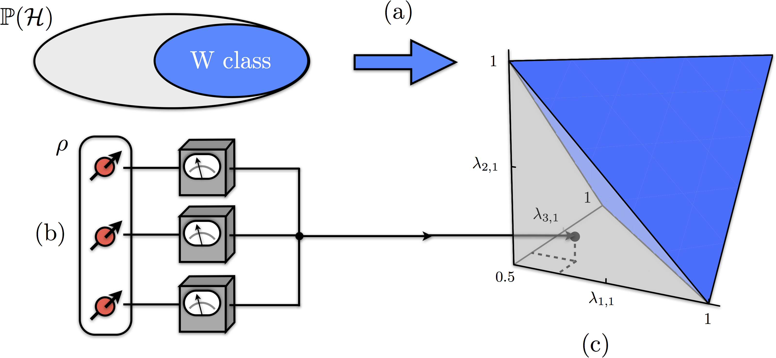
Figure 4.1: Entanglement polytopes as witnesses (illustrated for three qubits). (a) An entanglement polytope contains all possible local eigenvalues of states in the entanglement class and its closure (the W class and its polytope are shown in blue). (b) For a sufficiently pure quantum state $\rho$, local tomography is performed to determine its local eigenvalues. (c) The indicated eigenvalues are not compatible with the W polytope, hence $\rho$ must have GHZ-type entanglement.

Our approach to multipartite entanglement is based on establishing a connection to the one-body quantum marginal problem (Section 4.3). The crucial observation is that the one-body reduced density matrices $\rho_{1},\dots,\rho_{n}$ or, equivalently, their eigenvalues $\vec{\lambda}_{1},\dots,\vec{\lambda}_{n}$ alone can already give considerable information about the entanglement of the global state, provided that it is pure. To make this precise, we consider the set of local eigenvalues $\vec{\lambda}=(\vec{\lambda}_{1},\dots,\vec{\lambda}_{n})$ of the states in the closure $\overline{\mathcal{X}}$ of a given entanglement class $\mathcal{X}$. Surprisingly, this set also forms a convex polytope (i.e., it is the convex hull of finitely many such vectors), and we call it the entanglement polytope $\Delta_{\mathcal{X}}$ of the class. Entanglement polytopes immediately lead to a local criterion for witnessing multipartite entanglement: If the collection of eigenvalues $\vec{\lambda}$ of the one-body reduced density matrices of a pure quantum state $\rho=\lvert\psi\rangle\langle\psi\rvert$ does not lie in an entanglement polytope, then the given state cannot belong to the closure of the corresponding entanglement class $\mathcal{X}$ (Figure 4.1):

$$\vec{\lambda}=(\vec{\lambda}_{1},\dots,\vec{\lambda}_{n})\notin\Delta_{\mathcal{X}}\,\Longrightarrow\,\rho\notin\overline{\mathcal{X}}.$$ (4.1)

In other words, the criterion allows us to witness the presence of a highly entangled state by showing that its local eigenvalues are incompatible with all less-entangled classes. This way of reasoning is similar to the exclusion of a local hidden variable model by witnessing the violation of a Bell inequality. Strikingly, there are always only finitely many entanglement polytopes, and they naturally form a hierarchy: if a state in some class $\mathcal{X}$ can be approximated arbitrarily well by states from $\mathcal{Y}$ then $\Delta_{\mathcal{X}}\subseteq\Delta_{\mathcal{Y}}$. This reflects geometrically the fact that states in the second class are more powerful for quantum information processing.

To describe $\Delta_{\mathcal{X}}$ mathematically and establish these claims, we work in the framework of Chapter 2. Using the characterization of SLOCC operations as invertible local operators $g_{1}\otimes\dots\otimes g_{n}$ [DVC00], we find that the closure of an entanglement class is a projective subvariety of the space of pure states. Thus $\Delta_{\mathcal{X}}$ can be identified with its moment polytope, and the above-mentioned properties follow from the general theory. We explain how $\Delta_{\mathcal{X}}$ can in principle be computed using computational invariant theory [DK02].

We now illustrate the method with some examples taken from Section 4.4. For qubit systems, each one-body reduced density matrix $\rho_{k}$ has two eigenvalues, which are non-negative and sum to one; hence its spectrum is completely characterized by the maximal eigenvalue $\lambda_{k,1}$, which can take values in the interval $[0.5,1]$. In the case of three qubits, we may therefore regard the entanglement polytopes as subsets of three-dimensional space. There are two full-dimensional polytopes, as has already been observed in [HZG04]: one for the W class (the upper pyramid in Figure 4.1) and the other for the GHZ class (the entire polytope, i.e., the union of both pyramids). The tip of the upper pyramid constitutes a polytope by itself, indicating a product state. Three further one-dimensional polytopes are given by the edges emanating from this vertex. They correspond to the three possibilities of embedding an EPR pair $(\ket{00}+\ket{11})/\sqrt{2}$ into three qubits. Thus, eigenvalues in the interior of the polytope are compatible only with the W and GHZ classes, i.e., genuine three-partite entanglement. If the eigenvalues lie in the lower pyramid, $\lambda_{1,1}+\lambda_{2,1}+\lambda_{3,1}<2$, then by (4.1) the state cannot be contained in the closure of the $W$ class—we have witnessed GHZ-type entanglement.

In systems of 4 qubits, there exist 9 infinite families of entanglement classes, each described by up to three complex parameters [VDDMV02] that are not directly accessible; arguably, the complete classification is too detailed to be practical. In contrast, entanglement polytopes strike an attractive balance between coarse-graining and preserving structure (Figure 4.2): Up to permutations, there are 12 entanglement polytopes, 7 of which are full-dimensional and correspond to distinct types of genuine four-partite entanglement. One example is the 4-qubit W class: in complete analogy to the previous case, its polytope is an “upper pyramid” of eigenvalues that fulfill $\lambda_{1,1}+\lambda_{2,1}+\lambda_{3,1}+\lambda_{4,1}\geq 3$.

$\hphantom{x}\lambda_{4,1}=0.5$

$\hphantom{xx}\lambda_{4,1}=2/3$

$\hphantom{xxx.}\lambda_{4,1}=5/6$

$\hphantom{xxxx.}\lambda_{4,1}=1$

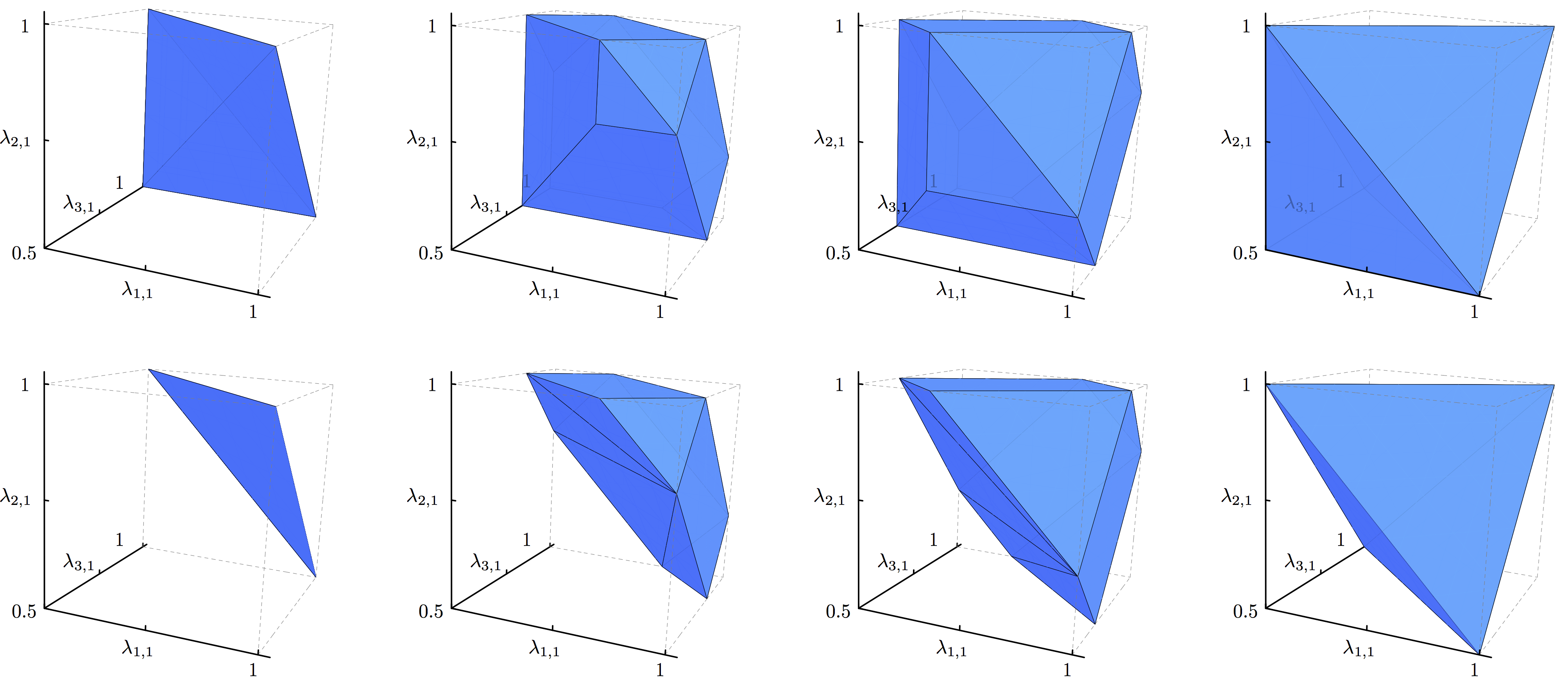
Figure 4.2: Cross-sections of two entanglement polytopes for four qubits. Each row shows cross-sections of a four-dimensional entanglement polytope for four fixed values of $\lambda_{4,1}$. The first row corresponds to the entanglement class $L_{a_{4}}$ for $a=0$ in the characterization of [VDDMV02], represented by the state $(i\ket{0001}+\ket{0110}-i\ket{1011})/\sqrt{3}$. The second row corresponds to the four-qubit W class, $(\ket{1000}+\dots+\ket{0001})/2$. One can clearly identify the “upper-pyramid form” explained in the text. Properties that had previously been computed algebraically can be read off directly: E.g., the final column corresponds to the situation when the fourth qubit has been projected onto a pure state; as apparent from the polytopes, the state of the remaining three sites is generically of GHZ type in the first row, and of W type in the second row. See [Wal12a] for an interactive visualization of all four-qubit entanglement polytopes.

In Section 4.4 we give further details on these computations. We also discuss the notion of genuinely multipartite entangled states, which are of particular interest [GTB05]. These are pure states which do not factorize with respect to any partition of the system into two sets of subsystems. We show for arbitrary systems that the entanglement polytopes of the biseparable states (i.e., the states that do factorize) do not account for all possible eigenvalues. Therefore, the presence of genuine multipartite entanglement in a pure quantum state can be witnessed by checking that the local eigenvalues do not lie in any biseparable polytope. We can also obtain more quantitative information about the multipartite entanglement of a quantum state, e.g., by witnessing genuine $k$-partite entanglement [GTB05] by using a generalization of the method sketched above. Entanglement polytopes can also be constructed for quantum systems composed of bosons or fermions [WDGC13].

In Section 4.5 we then consider the linear entropy of entanglement $E(\rho)=1-\frac{1}{n}\sum_{j=1}^{n}\operatorname{tr}\rho_{j}^{2}$ [ZHP93, BKO⁺04, BM08], used, e.g., in metrology [FNP98]. Entanglement polytopes allow us to bound the maximal linear entropy of entanglement distillable by SLOCC operations: Since $1-E(\rho)$ corresponds to the Euclidean length of the vector $\vec{\lambda}$ of local eigenvalues, shorter vectors imply more entanglement. In particular, quantum states of maximal entropy of entanglement in a class $\mathcal{X}$ map to the point of minimal distance to the origin in the entanglement polytope $\Delta_{\mathcal{X}}$. Therefore, if the local eigenvalues of a given state lie only in polytopes with small distance to the origin, a high amount of entanglement can be distilled. We explain how to turn this observation into a quantitative statement and describe a distillation procedure based on Kirwan and Ness’ gradient flow [Kir84a, NM84]. Intriguingly, we find that a generalization of this technique gives rise to a probabilistic classical algorithm for the computation of entanglement polytopes and, in fact, general moment polytopes of orbit closures (cf. [Wer13]).

Quantum states prepared in the laboratory are always subject to noise and therefore never perfectly pure. In Section 4.6 we show how our method for witnessing entanglement using (4.1) can be adapted to this situation as long as the noise is not too large. To make this statement precise, we assume that a lower bound $1-\varepsilon$ on the purity $\mathrm{tr}\,\rho^{2}$ of a quantum state $\rho$ is available. This implies that $\rho$ has fidelity $\langle\psi|\rho|\psi\rangle\geq 1-\varepsilon$ with a pure state $\lvert\psi\rangle$ whose local eigenvalues deviate from the measured ones by no more than a small amount $\delta(\varepsilon)$. In the case of $n$ qubits one has that $\delta(\varepsilon)\approx n\varepsilon/2$ for small impurities. Therefore, as long as the distance of the measured eigenvalues $\vec{\lambda}$ to an entanglement polytope $\Delta_{\mathcal{X}}$ is at least $\delta(\varepsilon)$, the experimentally prepared state $\rho$ has high fidelity with a pure state that is more entangled than the class $\mathcal{X}$. These ideas can be further extended to show that $\rho$ itself cannot be written as a convex combination of quantum states in a given entanglement class. Unlike the local eigenvalues, the purity $\mathrm{tr}\,\rho^{2}$ cannot be estimated by single-particle tomography alone. However, it is in general not necessary to perform full tomography of the global state in order to determine the purity [BCWdW01]. Whereas it is an experimental challenge to achieve the levels of purity necessary for the application of our method, we believe that they are in the reach of current technology [RNO⁺00, PDG⁺01, MSB⁺11].

After completion of the work described in this chapter, we have learned about independent related work by Sawicki, Oszmaniec and Kuś [SOK12b, SOK12a].

4.2 Classification of Entanglement

A pure quantum state $\rho=\lvert\psi\rangle\langle\psi\rvert$ of a multi-particle system with Hilbert space $\mathcal{H}=\mathcal{H}_{1}\otimes\dots\otimes\mathcal{H}_{n}$ is called entangled if it cannot be written as a tensor product [NC04]

$$\ket{\psi}\neq\ket{\psi_{1}}\otimes\dots\otimes\ket{\psi_{n}}.$$

It is easy to see that $\rho$ is unentangled, or separable, if and only if each its one-body reduced density matrices $\rho_{k}$ is itself a pure state. More generally, mixed states are called separable if they are convex combinations of product states, but in this chapter we are primarily concerned with the entanglement of pure states.

In order to classify the entanglement present in a given multipartite quantum state $\rho$, one fruitful approach has been to compare the capability of $\rho$ for quantum information processing tasks with that of other quantum states [BPR⁺00]. Specifically, suppose that $\rho^{\prime}$ is a state that can be obtained from $\rho$ by some suitable class of operations. Then $\rho$ can be used as a replacement for $\rho^{\prime}$ in any quantum information processing scenario where these operations are considered to be “free”. If the operations themselves cannot create entanglement then we may think of $\rho$ to be at least as entangled as $\rho^{\prime}$. If, conversely, $\rho$ can also be obtained from $\rho^{\prime}$ then we may regard the two states to possess the same kind of multipartite entanglement. In this way the set of quantum states is partitioned into equivalence classes.

For example, any local operation that only acts on one of the $n$ subsystems can never create entanglement. Local operations, including measurements, can be described by trace-preserving, completely positive maps that act on the space of density operators on $\mathcal{H}_{k}$. Conversely, Stinespring’s dilation theorem shows that such maps can always be implemented by locally adding an ancilla system, performing a unitary operation, and tracing out. It is also useful to allow for classical communication between the subsystems, which can create classical correlations but no entanglement. This allows to condition each subsequent operation on the outcomes of previous measurements, even if those were performed at different subsystems. To model this formally, one needs an additional, classical register that stores the measurement outcome (as opposed to the post-measurement state); this leads to the definition of a quantum instrument (see, e.g., the exposition in [CLM⁺14]). We thus obtain a class of operations known as local operations and classical communication, or LOCC. For mixed states, the resulting theory is rather rich and has been extensively studied in the literature (also asymptotically in the limit of many copies of a given state). For pure states, however, the resulting notion of LOCC equivalence is quite restrictive: Two pure states can be interconverted by LOCC if and only if they are related by local unitaries [Nie99, BPR⁺00].

In the context of this work it will thus be convenient to consider a stochastic version of LOCC, known as SLOCC [BPR⁺00, DVC00]. Here, the conversion of one state into another is only required to succeed with non-zero probability. Operationally, this amounts to allowing post-selection on measurement outcomes that occur with non-zero probability.

In [DVC00], it has been shown that two pure states $\rho=\lvert\psi\rangle\langle\psi\rvert$ and $\rho^{\prime}=\lvert\psi^{\prime}\rangle\langle\psi^{\prime}\rvert$ are interconvertible using SLOCC if and only if there exist invertible operators $g_{k}$ acting on $\mathcal{H}_{k}$ such that $\ket{\psi^{\prime}}=(g_{1}\otimes\dots\otimes g_{n})\ket{\psi}$. Here, the non-trivial part is to show that invertible operators $g_{k}$ can be constructed by following a successful branch of an SLOCC conversion protocol. For the converse, we may simply successively perform local POVM measurements with Kraus operators

$$S_{k}=\sqrt{p_{k}}g_{k},\leavevmode\nobreak\ F_{k}=\sqrt{\mathbbm{1}-p_{k}(g_{k})^{\dagger}g_{k}},$$ (4.2)

where $p_{k}>0$ is a suitable normalization constant such that $p_{k}g_{k}^{\dagger}g_{k}\leq\mathbbm{1}$. If all measurements succeed (corresponding to outcomes $S_{1},\dots,S_{n}$) then $\rho^{\prime}$ has been successfully distilled from $\rho$ [DVC00].

Mathematically, the result of [DVC00] can be phrased in terms of the action (2.11) of the Lie group $G=\operatorname{SL}(\mathcal{H}_{1})\times\dots\times\operatorname{SL}(\mathcal{H}_{n})$ on projective space $\mathbbm{P}(\mathcal{H})$: Two pure states $\rho$ and $\rho^{\prime}$ are interconvertible by SLOCC if and only if one state is contained in the $G$-orbit of the other, or, equivalently, if and only if the two orbits are the same: $G\cdot\rho=G\cdot\rho^{\prime}$. We take this as the definition of an entanglement class:

Definition .

Let $\mathcal{H}=\mathcal{H}_{1}\otimes\dots\otimes\mathcal{H}_{n}$ be a tensor-product Hilbert space. The (SLOCC) entanglement class of a pure state $\rho=\lvert\psi\rangle\langle\psi\rvert$ is defined as

$$\mathcal{X}_{\rho}:=G\cdot\rho=\left\{\frac{\Pi(g)\lvert\psi\rangle\langle\psi\rvert\Pi(g)^{\dagger}}{\braket{\psi}{\Pi(g)^{\dagger}\Pi(g)}{\psi}}:g\in G\right\}\subseteq\mathbbm{P}(\mathcal{H}).$$

In this way, the group $G$ that had already appeared in the preceding chapters acquires a physical interpretation in terms of SLOCC operations. It is clear that the product states form a single entanglement class. The closure of an entanglement class contains in addition to the class itself also those quantum states which can be arbitrarily well approximated by states in the class. It can thus be given a similar operational interpretation as the class itself. While the entanglement classes partition the set of multipartite quantum states, their closures naturally form a hierarchy. Indeed, it is immediate that $\rho^{\prime}\in\overline{\mathcal{X}_{\rho}}$ implies $\overline{\mathcal{X}_{\rho^{\prime}}}\subseteq\overline{\mathcal{X}_{\rho}}$. Every entanglement class contains in its closure the class of unentangled states.

Stochastic local operations and classical communication provide a systematic framework for studying multi-particle entanglement. However, it is immediate from the fact that the dimension of $G$ grows only linearly with the particle number $n$ that there is generically an infinite number of distinct SLOCC entanglement classes, labeled by an exponential number of continuous parameters (cf. Section 4.4). It is therefore necessary to coarsen the classification in a systematic way in order to arrive at a tractable way of witnessing multi-particle entanglement. This is one motivation for the notion of entanglement polytopes that we will define in the next section.

We conclude this section by noting that an extraordinary amount of research has been devoted to the classification of entanglement and its experimental identification. The field is far too large to allow for an exhaustive bibliography; we refer to [HHHH09, EG08] for reviews of the general theory and to [GT09] for a review focusing on detection. Methods from algebraic geometry and classical invariant theory have long been used to analyze entanglement classes, see, e.g., [VDDMV02, Kly02, BLT03, VDDM03, Miy03, LLW04, HZG04, OS05, OS06, Kly07, ĐO09, BKM⁺09, Ost10, GW11, VES11, EBOS12] and references therein.

4.3 Entanglement Polytopes

Let $\mathcal{H}=\mathcal{H}_{1}\otimes\dots\otimes\mathcal{H}_{n}$ and $G=\operatorname{SL}(\mathcal{H}_{1})\times\dots\times\operatorname{SL}(\mathcal{H}_{n})$. We are interested in studying the one-body reduced density matrices $\rho_{1},\dots,\rho_{n}$ for all pure states $\rho$ in a given entanglement class $\mathcal{X}\subseteq\mathbbm{P}(\mathcal{H})$ and its closure $\overline{\mathcal{X}}$. This is a refinement of the one-body quantum marginal problem, Chapter 2, where we had instead considered all pure states on $\mathcal{H}$. Since $G$ contains the maximal compact subgroup $K=\operatorname{SU}(\mathcal{H}_{1})\times\dots\times\operatorname{SU}(\mathcal{H}_{n})$ of local unitaries, we may – just as in the case of Chapter 2 – equivalently study the local eigenvalues $\vec{\lambda}_{k}$, as captured by the following definition:

Definition .

The entanglement polytope of an entanglement class $\mathcal{X}$ is

$$\Delta_{\mathcal{X}}=\left\{(\vec{\lambda}_{1},\dots,\vec{\lambda}_{n}):\vec{\lambda}_{k}=\operatorname{spec}\rho_{k},\rho\in\overline{\mathcal{X}}\right\},$$

the set of local eigenvalues of the one-body reduced density matrices of all quantum states in the closure of the entanglement class.

As $\overline{\mathcal{X}}$ is the closure of a $G$-orbit, it is a $G$-invariant projective subvariety of $\mathbbm{P}(\mathcal{H})$. Its moment polytope $\Delta_{K}(\overline{\mathcal{X}})=\mu_{X}(\overline{\mathcal{X}})\cap i\mathfrak{t}^{*}_{+}$ can be identified with $\Delta_{\mathcal{X}}$ in the same way as we did in Section 2.3 for the one-body quantum marginal problem. We summarize:

Lemma .

The set $\Delta_{\mathcal{X}}$ is a convex polytope that can be identified with the moment polytope $\Delta_{K}(\overline{\mathcal{X}})$ of the projective subvariety $\overline{\mathcal{X}}\subseteq\mathbbm{P}(\mathcal{H})$.

If the vector $\vec{\lambda}=(\vec{\lambda}_{1},\dots,\vec{\lambda}_{n})$ of local eigenvalues of a state $\rho$ is not contained in a given entanglement polytope $\Delta_{\mathcal{X}}$ then by definition $\rho$ cannot be contained in the closure of the class $\mathcal{X}$. This establishes (4.1), our criterion for witnessing multi-particle entanglement. The entanglement polytopes form a hierarchy which coarsens the hierarchy of the closures of entanglement classes:

$$\overline{\mathcal{X}}\subseteq\overline{\mathcal{Y}}\,\Longrightarrow\,\Delta_{\mathcal{X}}\subseteq\Delta_{\mathcal{Y}}$$

We remark that $\vec{\lambda}$ is a natural generalization of the Schmidt coefficients or entanglement spectrum for bipartite states.

As we saw in Chapter 2, the convexity of moment polytopes can be established for arbitrary $G$-invariant projective subvarieties of $\mathbbm{P}(\mathcal{H})$. For example, we may also consider the set $\{\rho=\rho_{I}\otimes\rho_{I^{c}}\}$ of pure states that are biseparable with respect to a fixed bipartition $I:I^{c}$ of the $n$ subsystems, known as a Segré variety in algebraic geometry. We will return to this construction in our discussion of genuine multipartite entanglement in Section 5.5.

We remark that subsequent works have proposed a similar analysis of entanglement based on entropies rather than eigenvalues, which leads to a coarser notion than our entanglement polytopes [HdV13, HPLdV13] (cf. Chapter 7).

Invariant-Theoretic Description

The convexity of moment polytopes and their description relies on the decomposition of the ring of regular functions into irreducible representations (Theorem 2.1). In the case of the closure of an entanglement class $\mathcal{X}=G\cdot\rho$, this description can be slightly simplified. For this, we consider the following definition from classical invariant theory [KP96].

Definition .

A covariant of degree $k$ and weight $\lambda=(\lambda_{1},\dots,\lambda_{n})$ is a $G$-equivariant map

$$\Phi\colon\mathcal{H}=\mathcal{H}_{1}\otimes\dots\otimes\mathcal{H}_{n}\longrightarrow V_{G,\lambda}=V^{d_{1}}_{\lambda_{1}}\otimes\dots\otimes V^{d_{n}}_{\lambda_{n}}$$

whose components are homogeneous polynomials of degree $k$ and where $d_{i}=\dim\mathcal{H}_{i}$.

Since $\Phi$ is homogeneous of degree $k$, we may think of each $\lambda_{i}$ as a Young diagram with $k$ boxes and at most $d_{i}$ rows, i.e., $\lambda_{i}\in\mathbbm{Z}_{\geq 0}^{d_{i}}$ and $\sum_{j}\lambda_{i,j}=k$ for all $i=1,\dots,n$. Indeed, this would be the only choice for the number of boxes if we were to work with $\operatorname{GL}(d_{1})\times\dots\times\operatorname{GL}(d_{n})$ rather than $G=\operatorname{SL}(d_{1})\times\dots\times\operatorname{SL}(d_{n})$. In the present context it is slightly more convenient to stay with the usual conventions and work with the latter group. A covariant for which $V_{G,\lambda}$ is the trivial representation is nothing but an invariant polynomial. This is the case if and only if each representation is a power of the determinant representation, i.e., if $\lambda_{i}=(k/d_{i},\dots,k/d_{i})$ for all $i=1,\dots,n$ (cf. Section 2.1). While covariants are functions defined on the Hilbert space $\mathcal{H}$, they are homogeneous and so their non-vanishing can be well-defined on points of projective space by taking any representative vector; we will denote this by $\Phi(\rho)\neq 0$.

The covariants of degree $k$ are in bijection with the highest weight vectors in $R_{k}(\mathcal{H})$, the space of homogeneous polynomials of degree $k$ on $\mathcal{H}$. Indeed, if $\Phi$ is a covariant of degree $k$ and weight $\lambda$ then its component

$$P\colon\mathcal{H}\rightarrow\mathbbm{C},\ket{\psi}\mapsto\bra{w_{0}\lambda}\Phi(\ket{\psi})$$ (4.3)

is a highest weight vector in $R_{k}(\mathcal{H})$ of highest weight $\lambda^{*}$, where $\ket{w_{0}\lambda}\in V_{G,\lambda}$ is a fixed “lowest weight vector” of weight $w_{0}\lambda=-\lambda^{*}$. What is more,

$$\Phi(\rho)\neq 0\;\Leftrightarrow\;P\big{|}_{\overline{G\cdot\rho}}\neq 0,$$ (4.4)

since the $G$-orbit through $\ket{w_{0}\lambda}$ spans the entire irreducible representation $V_{G,\lambda}$, while any polynomial that vanishes on $G\cdot\rho$ must also vanish on the closure. The following lemma is already implicit in [Bri87]:

Lemma .

For an entanglement class $\mathcal{X}=G\cdot\rho$, the following are equivalent:

1. There exists an irreducible representation $V_{G,\lambda^{*}}\subseteq R_{k}(\overline{\mathcal{X}})$.

2. There exists a covariant $\Phi$ of degree $k$ and weight $\lambda$ such that $\Phi(\rho)\neq 0$.

Proof.

$(1)\Rightarrow(2)$: Let $P$ denote a highest weight vector of the irreducible representation $V_{G,\lambda^{*}}\subseteq R_{k}(\overline{\mathcal{X}})$. Then we may consider $P$ as a polynomial in $R_{k}(\mathcal{H})$ that does not vanish on $\overline{\mathcal{X}}$, and (4.4) implies that the corresponding covariant $\Phi$ is non-zero at $\rho$.

$(2)\Rightarrow(1)$: Conversely, any covariant $\Phi$ with $\Phi(\rho)\neq 0$ corresponds to a highest weight vector $P$ of highest weight $\lambda^{*}$ in $R_{k}(\mathcal{H})$. By virtue of (4.4), $P$ does not fully vanish on $\overline{\mathcal{X}}$. Therefore, $P$ determines a highest weight vector in $R_{k}(\overline{\mathcal{X}})$ and there exists a corresponding irreducible representation $V_{G,\lambda^{*}}\subseteq R_{k}(\overline{\mathcal{X}})$. ∎

To show that moment polytopes are not only convex but indeed polytopes, we had used the crucial fact that the algebra of $N_{+}$-invariant polynomials $R(\mathcal{H})^{N_{+}}$ – whose elements are linear combinations of highest weight vectors – is finitely generated [Gro73] (see proof of Section 2.2). We saw that there exist finitely many highest weight vectors $P^{(1)},\dots,P^{(m)}$ such that all other highest weight vectors can be obtained as linear combinations of monomials in the $P^{(j)}$. Let us call the corresponding covariants $\Phi^{(1)},\dots,\Phi^{(m)}$ a generating set of covariants.

Proposition .

The entanglement polytope of an entanglement class $\mathcal{X}=G\cdot\rho$ is given by

$$\Delta_{\mathcal{X}}=\operatorname{conv}\left\{\frac{\lambda^{(j)}}{k^{(j)}}=\frac{(\lambda^{(j)}_{1},\dots,\lambda^{(j)}_{n})}{k^{(j)}}:\Phi^{(j)}(\rho)\neq 0\right\}.$$

where $\Phi^{(1)},\dots,\Phi^{(m)}$ denotes a generating set of covariants with degrees $k^{(j)}$ and weights $\lambda^{(j)}$.

Proof.

Recall from Section 4.3 that $\Delta_{\mathcal{X}}$ can be identified with the moment polytope of the $K$-action on $\overline{\mathcal{X}}$. By Theorem 2.1 and Section 4.3, the rational points of the entanglement polytope are thus given by the normalized weights $\lambda/k$ corresponding to covariants that do not vanish at $\rho$. In particular, the inclusion $(\supseteq)$ is immediate.

For $(\subseteq)$, we closely follow the proof of Section 2.2. Let $\lambda/k\in\Delta_{\mathcal{X}}$ with corresponding covariant $\Phi$ of degree $k$ and weight $\lambda$. We denote by $P\in R_{k}(\mathcal{H})$ the highest weight vector (4.3) corresponding to the covariant $\Phi$. Since the $P^{(j)}$ are generators of the algebra of highest weight vectors, we may write $P$ as a linear combination of monomials in the $P^{(j)}$. If the linear combination is chosen minimally then the degrees $k^{(j)}$ and weights $\lambda^{(j)}$ of each monomial $P^{(j_{1})}\dotsm P^{(j_{p})}$ add up to the degree $k$ and weight $\lambda$ of $P$. Thus,

$$\frac{\lambda}{k}=\sum_{i}\frac{k^{(j_{i})}}{k}\frac{\lambda^{(j_{i})}}{k^{(j_{i})}}\in\operatorname{conv}\left\{\frac{\lambda^{(j_{1})}}{k^{(j_{1})}},\dots,\frac{\lambda^{(j_{p})}}{k^{(j_{p})}}\right\}$$ (4.5)

We know from (4.4) that $P$ does not completely vanish on $\mathcal{X}$. Thus same must be true for all factors in at least one of the monomials in the linear combination. Again using (4.4), the corresponding covariants $\Phi^{(j_{1})},\dots,\Phi^{(j_{p})}$ are all non-zero at $\rho$. But then (4.5) shows that $\lambda/k$ is indeed a convex combination of normalized weights $\lambda^{(j)}/k^{(j)}$ of non-vanishing covariants. ∎

Finite generation also implies other desirable properties, which hold more generally for moment polytopes of projective subvarieties [Bri87]. For example, there are only finitely many entanglement polytopes, since by Section 4.3 any entanglement polytope is the convex hull of some subset of the finite list of normalized weights $\lambda^{(j)}/k^{(j)}$. What is more, the set of quantum states for which all generators are non-zero,

$$\bigcap_{j=1}^{m}\{\rho\in\mathbbm{P}(\mathcal{H}):\Phi^{(j)}(\rho)\neq 0\},$$

is a finite intersection of Zariski-open sets, hence itself Zariski-open. In particular, its complement has positive codimension. It follows that the entanglement polytope of a generic quantum state is maximal and equal to

$$\operatorname{conv}\{\lambda^{(j)}/k^{(j)}:j=1,\dots,m\}$$

$$= \overline{\{\lambda/k:\text{ $\exists$ covariant of degree $k$ and weight $\lambda$}\}}$$

$$= \overline{\{\lambda/k:\text{ $\exists$ }V_{G,\lambda^{*}}\subseteq R_{k}(\mathcal{H})\}}$$

$$= \Delta_{K}(\mathbbm{P}(\mathcal{H})),$$

which we recognize as the solution of the one-body quantum marginal problem for pure-states on $\mathcal{H}$.

We stress that this observation does not imply that the method is trivial. Even if mathematically a given entanglement class has measure zero in projective space, it can still be an important task to show that a quantum state prepared in the laboratory is not contained in the class—this is perhaps most obvious if the class is the set of separable pure states! In our approach, this can be done using criterion (4.1) by showing that the local eigenvalues of the state are sufficiently far away from the entanglement polytope of the class. As we explain in Section 4.6, in the presence of small noise our method can be adapted to exclude convex combinations of classes (which always have positive measure). We remark that in classical statistics, testing for non-independence of random variables is similarly concerned with rejecting a measure-zero property (with respect to the natural measure on the probability simplex of joint distributions).

Computation

By virtue of Section 4.3, the computation of entanglement polytopes is a finite problem that can in principle be completely algorithmized. By using the relation

$$R(\mathcal{H})^{N_{+}}\cong\left(R(\mathcal{H})\otimes R(G)^{N_{+}}\right)^{G}\cong R(\mathcal{H}\times G/N_{+})^{G},$$

which is in fact at the heart of the proof of finite generation [Gro73], the problem of computing a set of generating covariants is transformed into a problem of computing invariants for a complex reductive group (see [Dol03, §4.2] for details; cf. [DK07]). For the latter problem there exists a Gröbner-basis algorithm in computational invariant theory [DK02] that has been implemented, e.g., in the Magma computer algebra system [BCP97] (but see Section 4.7). Once a set of generating covariants has been found, Section 4.3 can be used to compute the entanglement polytope both for specific states as well as for families of states. We demonstrate this method when computing examples in the next section (relying on generating sets of covariants that had been previously computed). In Section 4.5 we describe an alternative approach that does not rely on computational invariant theory.

4.4 Examples

In the preceding section we have seen that by associating to every entanglement class its entanglement polytopes we obtain a finite yet systematic classification of multipartite entanglement. We will now discuss some illustrative examples for qubit systems, where the Hilbert space is of the form $\mathcal{H}=\mathbbm{C}^{\otimes 2}\otimes\dots\otimes\mathbbm{C}^{\otimes 2}$. Mathematically, the covariants of a multi-qubit system are in one-to-one correspondence with the covariants of binary multilinear forms, which have been intensely studied in classical invariant theory [Olv99, Luq07].

Before we proceed, we introduce some notational simplifications. It will be convenient to represent the local eigenvalues of a pure state of $n$ qubits by the tuple $(\lambda_{1,1},\dots,\lambda_{n,1})\in[0.5,1]^{n}$ of maximal local eigenvalues; this is without loss of information since the eigenvalues of the one-body reduced density matrix of each qubit sum to one. Thus a covariant of degree $k$ and weight $(\lambda_{1},\dots,\lambda_{n})$ determines the point $(\lambda_{1,1},\dots,\lambda_{1,n})/k$ in the polytope of maximal local eigenvalues.

Two Qubits

We briefly discuss the rather trivial case of two qubits, where $\mathcal{H}=\mathbbm{C}^{2}\otimes\mathbbm{C}^{2}$. Here there are two entanglement classes: One class is represented by the maximally entangled Einstein–Podolsky–Rosen (EPR) pair

$$\ket{\operatorname{EPR}}=(\ket{00}+\ket{11})/\sqrt{2},$$

the other is the class of product states, represented by $\ket{00}$. Using Chapter 2, it is not hard to see that the entanglement polytope of the former class is given the convex hull of $(0.5,0.5)$ and $(1,1)$, while the entanglement polytope of the product states is a single point $(1,1)$. We can also see this formally by using the method of covariants. There are two generating covariants: One is the identity map

$$\mathbbm{C}^{2}\otimes\mathbbm{C}^{2}\rightarrow V^{2}_{\Yboxdim{5pt}\yng(1)\Yboxdim{8pt}}\otimes V^{2}_{\Yboxdim{5pt}\yng(1)\Yboxdim{8pt}},$$

which never vanishes and therefore shows that the point $(1,1)$ is contained in both entanglement polytopes. The other is the map

$$\mathbbm{C}^{2}\otimes\mathbbm{C}^{2}\rightarrow V^{2}_{\Yboxdim{5pt}\yng(1,1)\Yboxdim{8pt}}\otimes V^{2}_{\Yboxdim{5pt}\yng(1,1)\Yboxdim{8pt}}\cong\mathbbm{C},\quad\ket{\psi}=\sum_{i,j}\psi_{ij}\ket{ij}\mapsto\psi_{00}\psi_{11}-\psi_{10}\psi_{01}$$

that sends a quantum state to the determinant of its coefficients. It is of degree 2 and therefore corresponds to the point $(0.5,0.5)$ in an entanglement polytope. Since the determinant is zero on the class of product states but not on the EPR pair, we obtain the two entanglement polytopes from above by using Section 4.3.

Three Qubits

5pt Covariant Degree Weight $\ket{\operatorname{GHZ}}$ $\ket{W}$ $\ket{B1}$ $\ket{B2}$ $\ket{B3}$ $\ket{\operatorname{SEP}}$ $f$ $1$ $(\yng(1),\yng(1),\yng(1))$ $\times$ $\times$ $\times$ $\times$ $\times$ $\times$ $H_{x}$ $2$ $(\yng(2),\yng(1,1),\yng(1,1))$ $\times$ $\times$ $\times$ $H_{y}$ $2$ $(\yng(1,1),\yng(2),\yng(1,1))$ $\times$ $\times$ $\times$ $H_{z}$ $2$ $(\yng(1,1),\yng(1,1),\yng(2))$ $\times$ $\times$ $\times$ $T$ $3$ $(\yng(2,1),\yng(2,1),\yng(2,1))$ $\times$ $\times$ $\Delta$ $4$ $(\yng(2,2),\yng(2,2),\yng(2,2))$ $\times$ 8pt

Table 4.1: Three-qubit covariants [LP81, Luq07]. Degrees and weights of a generating set of three-qubit covariants labeled as in [Luq07, p. 31], as well as their vanishing behavior on the quantum states representing the six entanglement classes described in the text ($\times$ denotes non-vanishing). The invariant $\Delta$ is Cayley’s hyperdeterminant, which is closely related to the 3-tangle [CKW00, Miy03].

In the case of three qubits, where $\mathcal{H}=\mathbbm{C}^{2}\otimes\mathbbm{C}^{2}\otimes\mathbbm{C}^{2}$, there are six distinct entanglement classes [DVC00]: The classes of the Greenberger–Horne–Zeilinger (GHZ) state [GHZ89] and of the W state [DVC00], respectively,

$$\ket{\operatorname{GHZ}} =(\ket{000}+\ket{111})/\sqrt{2},$$

$$\ket{W} =(\ket{100}+\ket{010}+\ket{001})/\sqrt{3},$$

three classes that correspond to EPR pairs shared between any two of the three subsystems,

$$\ket{B1} =(\ket{010}+\ket{001})/\sqrt{2},$$

$$\ket{B2} =(\ket{100}+\ket{001})/\sqrt{2},$$

$$\ket{B3} =(\ket{100}+\ket{010})/\sqrt{2},$$

and the class of product states, represented by

$$\ket{\operatorname{SEP}}=\ket{000}.$$

We shall now compute the corresponding entanglement polytopes by following the general method of covariants described in Section 4.3. A minimal generating set of six covariants has been determined in late 19th century invariant theory [LP81] in the context of the classification of binary three-linear forms, as explained in [Luq07]. Recall that each irreducible representation $V^{2}_{\mu}$ of $\operatorname{SU}(2)$ can be realized as the space of homogeneous polynomials of degree $\mu_{1}-\mu_{2}$ in two formal variables. Therefore, any covariant for three qubits can be written as a homogeneous polynomial in formal variables $x_{i}$, $y_{j}$ and $z_{k}$, whose coefficients are themselves homogeneous polynomials in the components $\psi_{ijk}$ of the quantum state (the degree in the $\psi_{ijk}$ is equal to the degree of the covariant, whereas the degrees in the formal variables determine its weight). For example, the identity map can be written as the multilinear polynomial $f=\sum_{i,j,k}\psi_{ijk}x_{i}y_{j}z_{k}$; it is a generating covariant of degree $1$ and weight $({\Yboxdim{5pt}\yng(1)\Yboxdim{8pt}},{\Yboxdim{5pt}\yng(1)\Yboxdim{8pt}},{\Yboxdim{5pt}\yng(1)\Yboxdim{8pt}})$. A more interesting generator is the covariant

$$H_{x} =x_{0}^{2}\left(\psi_{000}\psi_{011}-\psi_{001}\psi_{010}\right)$$

$$+x_{1}x_{0}\left(\psi_{011}\psi_{100}-\psi_{010}\psi_{101}-\psi_{001}\psi_{110}+\psi_{000}\psi_{111}\right)$$

$$+x_{1}^{2}\left(\psi_{100}\psi_{111}-\psi_{101}\psi_{110}\right)$$

which is of degree $2$ and weight $({\Yboxdim{5pt}\yng(2)\Yboxdim{8pt}},{\Yboxdim{5pt}\yng(1,1)\Yboxdim{8pt}},{\Yboxdim{5pt}\yng(1,1)\Yboxdim{8pt}})$. We refer to [Luq07, p. 31] for the complete list. By Section 4.3, computing the entanglement polytopes is now a mechanical task: for any quantum state representing the entanglement class, we merely need to collect those covariants which do not vanish on the state, and take the convex hull of their normalized weights. In Table 4.1 we have summarized the covariants’ properties and their vanishing behavior on the six entanglement classes. The resulting entanglement polytopes are illustrated in Figure 4.3. They are in one-to-one correspondence with the six entanglement classes described above. Since only the GHZ-class polytope is maximal, it follows that all states can be approximated arbitrarily well by states of GHZ type. In mathematical terms, the GHZ class is dense; this is of course well-known [DVC00]. Similarly, the polytope of the W class (upper pyramid) contains all entanglement polytopes except for the GHZ one; and it is easy to see that by states in the W class one can approximate all states except those of GHZ class. Thus in this low-dimensional scenario the hierarchy of closures of entanglement classes is faithfully mapped onto the hierarchy of entanglement polytopes—there is no coarse-graining.

(a)xxxxx

(b)xxxx

(c)xxx

(d)xx

Figure 4.3: Entanglement polytopes for three qubits. (a) GHZ polytope (maximal polytope, i.e., upper and lower pyramid), (b) W polytope (upper pyramid), (c) three polytopes corresponding to EPR pairs shared between any two of the three parties (three solid edges in the interior), (d) polytope of the unentangled states (interior vertex).

We remark that using techniques crafted towards the special situation of three qubits, these same polytopes had already been previously computed in [HZG04, SWK13]. The one-body quantum marginal problem, which as we have explained amounts to computing the maximal entanglement polytope, has been solved in [HSS03], and we saw a different derivation in Chapter 3.

We now illustrate the method of entanglement witnessing via (4.1). Let $\rho$ be a quantum state with maximal local eigenvalues $\vec{\lambda}=(\lambda_{1,1},\lambda_{2,1},\lambda_{3,1})$.

• If the point $\vec{\lambda}$ is contained in the lower part of the entanglement polytope of the GHZ class (lower pyramid in Figure 4.3, (a)),

  $$\lambda_{1,1}+\lambda_{2,1}+\lambda_{3,1}<2,$$

  then it is not contained in any other entanglement polytope. Therefore the quantum state $\rho$ must be entangled of GHZ type.

• More generally, if $\vec{\lambda}$ is not contained in any of the lower-dimensional polytopes corresponding to EPR pairs (Figure 4.3, (c), which includes (d)), i.e., if

  $$\lambda_{k,1}<1\quad(\forall k=1,2,3),$$

  then the quantum state $\rho$ must be entangled of either GHZ or W class. These classes of states are the ones that possess genuine three-qubit entanglement (see discussion below).

As a final example, we consider the quantum state $\rho=\lvert\psi\rangle\langle\psi\rvert$, where

$$\ket{\psi}=(\ket{000}+\ket{001}+\ket{100}+2\ket{110})/\sqrt{7}.$$ (4.6)

It is easy to verify by the method of covariants that the entanglement polytope of $\rho$ is full-dimensional. Thus it follows from the above classification that $\rho$ is of GHZ type. However, its collection of local eigenvalues $(\lambda_{1,1},\lambda_{2,1},\lambda_{3,1})\approx(0.76,0.79,0.88)$ is contained in the interior of the upper pyramid. As we just discussed, the entanglement criterion in this case only allows us to conclude that $\rho$ is either of GHZ or of W type. In Section 4.5 we will describe a distillation procedure that allows us to transform $\rho$ by SLOCC operations into another state whose local eigenvalues are arbitrarily close to the “origin” $(0.5,0.5,0.5)$ (cf. Figure 4.6). In this way, we may arrive at a quantum state which is both more entangled and for which the entanglement criterion is maximally informative.

Four Qubits

In contrast to case of three qubits, where there are finitely many entanglement classes represented faithfully by the hierarchy of entanglement polytopes, the situation for four qubits is the generic one: There are infinitely many entanglement classes. According to the classification of [VDDMV02], up to permutation of the qubits they can be partitioned into nine families with up to three complex continuous parameters each (cf. [CD07]). Neither the family itself nor the complex parameters within a family are directly experimentally accessible.

We have determined all entanglement polytopes of four qubits using the general method of Section 4.3 applied to a minimal generating set of 170 covariants found in [BLT03]. More precisely, for every family in [VDDMV02], we consider the covariants as a function of the parameters $a$, $b$, etc. of the family. Deciding whether a normalized weight $\lambda^{(j)}/k^{(j)}$ is included in the entanglement polytope $\Delta_{\mathcal{X}}$ of a state in the family then amounts to solving the explicit polynomial equation $P_{j}\neq 0$ in the parameters $a$, $b$, etc.; this can be automatized by using a computer algebra system.

The maximal entanglement polytope is equal to the solution of the one-body quantum marginal problem for four qubits as given by the polygonal inequalities (3.2) for $n=4$. It is a convex hull of 12 vertices, which can be easily described as follows: One vertex, $(1,1,1,1)$ corresponds to the class of product states; $(0.5,0.5,1,1)$ and its permutations correspond to the six possibilities of embedding an EPR pair into four qubits; $(0.5,0.5,0.5,1)$ and its permutations correspond to the four possibilities of embedding a GHZ state of three qubits; and the vertex $(0.5,0.5,0.5,0.5)$ is the image of, e.g., a four-partite GHZ state.

As in the case of three qubits, there are several lower-dimensional entanglement polytopes, corresponding to the different ways of embedding entanglement classes of systems of fewer qubits into four qubits. These are precisely the biseparable entanglement classes, i.e., the classes whose elements are tensor products $\rho=\rho_{I}\otimes\rho_{I^{c}}$ with respect to some proper bipartition $I:I^{c}$ of the four qubits. For example, the state $\ket{\operatorname{GHZ}}\otimes\ket{0}$ generates an entanglement class whose elements are tensor products of the three-qubit GHZ class and a one-qubit pure state, and its entanglement polytope is the Cartesian product of the three-qubit GHZ polytope with the point $\{1\}$. All possibilities are listed in Table 4.2.

Representative State	Number of Embeddings	Dimension
$\ket{\operatorname{GHZ}}\otimes\ket{0}$	4	3
$\ket{W}\otimes\ket{0}$	4	3
$\ket{\operatorname{EPR}}\otimes\ket{\operatorname{EPR}}$	3	2
$\ket{\operatorname{EPR}}\otimes\ket{0}\otimes\ket{0}$	6	1
$\ket{0}\otimes\ket{0}\otimes\ket{0}\otimes\ket{0}$	1	0

Table 4.2: Biseparable entanglement classes of four-qubit states. Each biseparable entanglement class is obtained by embedding entanglement classes of fewer qubits. In the left column, we give a representative state for each class; the middle column lists the number of permutations of qubits that lead to distinct embeddings, and hence to distinct polytopes, and the right column lists the dimension of the polytope.

We now turn to the full-dimensional polytopes. There are seven such polytopes, listed together with some of their properties in Table 4.3 and Figure 4.4. For example, the entanglement classes of the four-qubit GHZ state and of the cluster states [BR01] are both associated with the maximal polytope (last row in Table 4.3 and Figure 4.4). The four-qubit $W$-state, $\ket{W_{4}}=(\ket{0001}+\ket{0010}+\ket{0100}+\ket{1000})/2$, corresponds to polytope no. 5 in Table 4.3 and Figure 4.4. In analogy with the $W$-state for three qubits, its polytope is an “upper pyramid” given by the intersection of the maximal polytope with the half-space

$$\lambda_{1,1}+\lambda_{2,1}+\lambda_{3,1}+\lambda_{4,1}\geq 3.$$

Any violation of this inequality may be taken as an indication of “high entanglement”. One way to make this precise is to read off Table 4.3 that violations imply that the state $\rho$ can be converted into one whose linear entropy of entanglement is at least $0.45$, which might be much higher than $E(\rho)$ itself. We will explain this more carefully in Section 4.5 below.

No	Family	Parameters	Vertices	Facets	Perms	$E(\Delta_{\mathcal{X}})$
1	$L_{0_{7\oplus\bar{1}}}$		12	13	4	0.482143
2	$L_{0_{5\oplus 3}}$		10	13	4	0.458333
3	$L_{a_{4}}$	$a=0$	9	14	6	0.45
4	$L_{abc_{2}}$	$a=c=0,b\neq 0$	8	16	1	0.5
5	$L_{ab_{3}}$	$b=a=0$	7	9	1	0.375
6	$L_{a_{2}b_{2}}$	$b=-a\neq 0$	10	14	6	0.5
7	$G_{abcd}$	generic	12	12	1	0.5

No	Vertices compared to maximal polytope
1	$(0.5,0.5,0.5,0.5)$ replaced by $(0.75,0.5,0.5,0.5)$
2	$(0.5,0.5,0.5,0.5),(1,0.5,0.5,0.5)$ missing
3	$(0.5,0.5,0.5,0.5),(0.5,1,0.5,0.5),(0.5,0.5,0.5,1)$ missing
4	$(0.5,0.5,0.5,1)$ and permutations missing
5	$(0.5,0.5,0.5,0.5)$, $(0.5,0.5,0.5,1)$ and permutations missing
6	$(0.5,1,0.5,0.5),(0.5,0.5,0.5,1)$ missing
7	(this is the maximal polytope)

Table 4.3: Entanglement polytopes for genuinely four-partite entangled states. For each polytope, the second and third column specifies one choice of family and parameters according to the classification of [VDDMV02] (there might be further choices, in part because their parametrization is not always unique). “Perms” is the number of distinct polytopes one obtains when permuting the qubits. $E(\Delta_{\mathcal{X}})$ is the maximal linear entropy of entanglement of any state in the class. The bottom table describes how to obtain each polytope from the maximal entanglement polytope (the solution of the one-body quantum marginal problem).

We now comment on properties that can be read off graphically from Figure 4.4. From the first column, one can see that only three of the entanglement polytopes (no. 4, 6 and 7) include the “origin” $(0.5,0.5,0.5,0.5)$. These reach the maximal value for the linear entropy of entanglement $E(\rho)=1-\frac{1}{n}\sum_{j=1}^{n}\operatorname{tr}\rho_{j}^{2}$. The last column exhibits the behavior of the class when the fourth particle is projected onto a generic pure state. We then obtain a pure state of three qubits on the remaining subsystems. Polytopes no. 1, 3, 6, and 7 give the full three-qubit polytope, implying that in general a GHZ-type state is generated, while polytopes no. 2, 4, and 5 collapse to the upper pyramid of Figure 4.1. Hence states in the latter classes can never product a state of GHZ-type when the fourth qubit is projected onto a pure state. It follows that the mixed 3-tangle (and any other convex-roof extension of a polynomial monotone) vanishes on the mixed state generated by tracing out the last particle of any state in these classes. This observation allows us to graphically recover some properties calculated algebraically in [VDDMV02], such as the vanishing 3-tangle for the class $L_{{ab}_{3}},a=b=0$ (corresponding to polytope no. 5).

$\lambda_{4,1}=0.5$

$\hphantom{x}\lambda_{4,1}=2/3$

$\hphantom{xx}\lambda_{4,1}=5/6$

$\hphantom{xxx}\lambda_{4,1}=1$

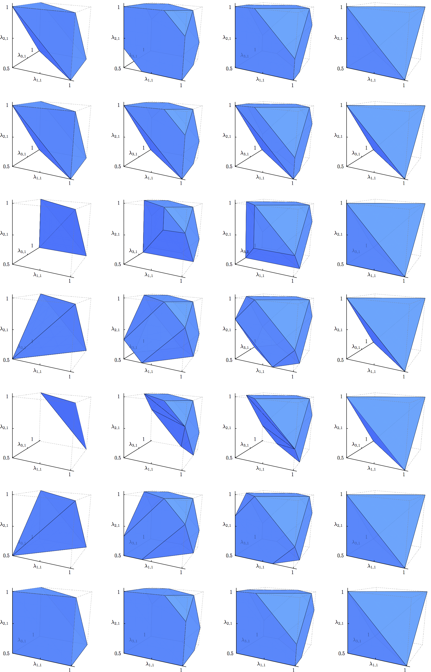
Figure 4.4: Illustration of the full-dimensional entanglement polytopes for four qubits. The seven rows correspond to the four-dimensional entanglement polytopes in Table 4.3. The four columns show cross-sections for four fixed values of $\lambda_{4,1}$.

In summary, up to permutations, there are 12 entanglement polytopes for four qubits, 7 of which are full-dimensional and belong to genuinely four-partite entangled states. These numbers increase to 41 and 22, respectively, if distinct permutations are counted separately. Slightly abusing the tradition of [DVC00, VDDMV02], we might say that from the perspective of entanglement polytopes, four qubits can be entangled in seven different ways.

We remark that there is a numerical coincidence between our findings and the ones in [ĐO09], where also seven non-biseparable entanglement classes have been identified on four qubits. The two classifications are, however, not identical. Indeed, [ĐO09] is based purely on invariants, as opposed to the more general covariant-theoretic description of our polytopes. It follows from Section 4.3 – as we discuss in Section 4.5 below – that all polynomial invariants vanish identically on any entanglement class whose polytope does not contain the “origin” $(0.5,0.5,0.5,0.5)$. Since this is the case for our polytopes no. 1, 2, 3 and 5, the corresponding classes cannot be distinguished from each other by polynomial invariants (in fact, not even from the class of product states!) Thus our classification differs from the one in [ĐO09]. From a mathematical perspective, our methods are complementary (entanglement polytopes can also distinguish among unstable vectors, whereas [ĐO09] provides a better resolution in the semistable case).

Genuine Multipartite Entanglement

In the preceding examples, entanglement classes corresponding to biseparable states, i.e., pure states that can be factorized in the form $\rho=\rho_{I}\otimes\rho_{I^{c}}$, had polytopes of lower dimension. This is no longer true for $n\geq 6$ particles. For example, the entanglement polytope $\Delta_{\operatorname{GHZ}}\times\Delta_{\operatorname{GHZ}}\subseteq[0.5,1]^{6}$ associated with the biseparable state $\ket{\operatorname{GHZ}}\otimes\ket{\operatorname{GHZ}}\in\mathbbm{C}^{\otimes 6}$ of six qubits is certainly six-dimensional.

Perhaps surprisingly, it still remains true that spectral information alone can be used to show that a state is not biseparable. To make this precise, we consider the following definition from [GTB05]; see also [HHH01, HHHH09, GT09, LM13, SU01, HMGH10] and references therein.

Definition .

Let $\mathcal{H}=\mathcal{H}_{1}\otimes\dots\otimes\mathcal{H}_{n}$. A pure state $\rho=\lvert\psi\rangle\langle\psi\rvert$ on $\mathcal{H}$ is called producible using $k$-partite entanglement if it is of the form

$$\rho=\rho_{I_{1}}\otimes\dots\otimes\rho_{I_{m}},$$

where $I_{1}\cup\dots\cup I_{m}=\{1,\dots,n\}$ and each subset $I_{j}$ is of size at most $k$.

Otherwise, $\rho$ is called genuinely $(k+1)$-partite entangled. In particular, the genuinely $n$-partite entangled states are precisely those which are not biseparable.

We remark that some authors use the term “genuine $n$-partite entanglement” in a different sense (e.g., [OS05, OS06] where it is also required that there exists a non-vanishing invariant polynomial).

To state our result, recall that the maximal entanglement polytope for $n$ qubits is given by the polygonal inequalities (3.2). Therefore, the constraints on the local eigenvalues of states that factorize with respect to a fixed partition $I_{1}\cup\dots\cup I_{m}=\{1,\dots,n\}$ are given by

$$\sum_{l\neq k\in I_{j}}\lambda_{k,1}\leq\left(\lvert I_{j}\rvert-2\right)+\lambda_{l,1}\quad(\forall l\in I_{j},j=1,\dots,m)$$ (4.7)

Mathematically, while this set of states does not form a single entanglement class, it is still a $G$-invariant projective subvariety – known as a Segré variety in algebraic geometry –, and so has a corresponding moment polytope, namely the one cut out by the inequalities (4.7). The inequalities (4.7) hold for quantum states of arbitrary local dimension, since the same is true for the polygonal inequalities, but in general there are additional constraints.

Proposition .

Let $n\geq 3$ and $k\in\{\lceil n/2\rceil,\dots,n\}$. For any $\varepsilon\in(0,1/(2k-2)]$, the local eigenvalues

$$\lambda_{1,1}=1-(k-1)\varepsilon,\quad\lambda_{2,1}=\dots=\lambda_{n,1}=1-\varepsilon$$

can only originate from a genuinely $k$-partite entangled state.

Conversely, if $k\neq n-1$ then there exists a corresponding pure state of $n$ qubits that is producible using $k$-partite entanglement (i.e., that is not genuinely $k+1$-partite entangled).

Proof.

For the first claim, suppose that $\rho=\rho_{I_{1}}\otimes\dots\otimes\rho_{I_{m}}$ is a state with the displayed local eigenvalues. Without loss of generality, suppose that $1\in I_{1}$. Then (4.7) for $l=1$ reads

$$\big{(}\lvert I_{1}\rvert-1\big{)}\big{(}1-\varepsilon\big{)}\leq\big{(}\lvert I_{1}\rvert-2\big{)}+\big{(}1-(k-1)\varepsilon\big{)}\quad\Leftrightarrow\quad\lvert I_{1}\rvert\geq k.$$ (4.8)

Since this holds for all partitions, we conclude that $\rho$ is genuinely $k$-partite entangled.

For the second claim, consider the bipartition $I_{1}=\{1,\dots,k\}$, $I_{2}=\{k+1,\dots,n\}$. Then (4.8) is satisfied and all other inequalities in (4.7) are satisfied for $I_{1}$ since $k\geq\lceil n/2\rceil\geq 2$. For $I_{2}$, which we need to consider only if $k<n$, (4.7) is equivalent to $k\leq n-2$. ∎

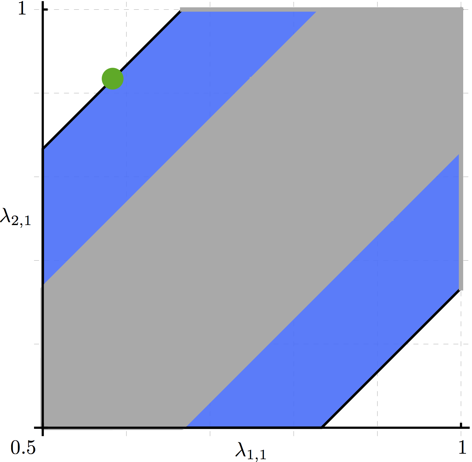
Figure 4.5: Witnessing genuine multipartite entanglement. The figure displays the two-dimensional cross-section through the six-qubit eigenvalue polytope (blue) and the biseparable subpolytopes (gray), where we fix $\lambda_{3,1}=\dots\lambda_{6,1}=11/12$. Any global pure state for which the local eigenvalues do not belong to the latter is necessarily genuinely six-qubit entangled. The spectrum produced by Section 4.4 for $k=n=6,\varepsilon=1/12$ is one such example (green point).

Section 4.4 shows that some correlations between the one-body reduced density matrices of a global pure state can only be explained by the presence of genuine $n$-partite entanglement. Since the complement of the union of biseparable entanglement polytopes is open, the first claim in the proposition is in fact true for a small ball around the eigenvalues (intersected with the overall polytope). See Figure 4.5 for an illustration.

4.5 Gradient Flow

The Role of the Origin

In Section 2.2 we had seen that the pure states $\rho$ whose one-body reduced density matrices are maximally mixed, $\rho_{1},\dots,\rho_{n}\propto\mathbbm{1}$, play a special mathematical role in geometric invariant theory. Some of their properties can be reinterpreted from the perspective of entanglement theory. For example, let $P$ be a $G$-invariant homogeneous polynomial and

$$M\colon\mathbbm{P}(\mathcal{H})\rightarrow\mathbbm{R}_{\geq 0},\rho=\lvert\psi\rangle\langle\psi\rvert\mapsto\lvert P(\ket{\psi})\rvert^{2}$$ (4.9)

the corresponding entanglement monotone [VDDM03]. Then $P$ attains at $\rho$ its maximal value over all states in the entanglement class $\mathcal{X}_{\rho}=G\cdot\rho$ [Kly07]. To see this, recall from (2.7) that for a locally maximally mixed state $\rho=\lvert\psi\rangle\langle\psi\rvert$ the norm square of the corresponding vector $\ket{\psi}$ does not change to first order as we move along the $G$-orbit in Hilbert space; that is $\ket{\psi}$ is a critical point of $\lVert-\rVert^{2}$ on its $G$-orbit. Kempf and Ness have shown that in fact any such vector has minimal length in its $G$-orbit [KN79], so that $\lVert\Pi(g)\ket{\psi}\rVert\geq\lVert\ket{\psi}\rVert=1$ for all $g\in G$. Thus,

$$M(\rho)=\lVert\Pi(g)\ket{\psi}\rVert^{k}\lvert P\left(\frac{\Pi(g)\ket{\psi}}{\lVert\Pi(g)\ket{\psi}\rVert}\right)\rvert\geq\lvert P\left(\frac{\Pi(g)\ket{\psi}}{\lVert\Pi(g)\ket{\psi}\rVert}\right)\rvert=M(g\cdot\rho),$$

where $k$ is the degree of $P$.

From the perspective of entanglement polytopes, locally maximally mixed quantum states correspond to the point

$$\vec{O}=(\underbrace{\frac{1}{d_{1}},\dots,\frac{1}{d_{1}}}_{d_{1}},\dots,\underbrace{\frac{1}{d_{n}},\dots\frac{1}{d_{n}}}_{d_{n}}),$$

which we will call the origin. We have used $\vec{O}$ as the origin of the coordinate systems in most of the figures in this chapter. Indeed, if we identify an entanglement polytope $\Delta_{\mathcal{X}}$ with the corresponding moment polytope $\Delta_{K}(\overline{\mathcal{X}})$ then the origin $\vec{O}$ corresponds to the point $0\in i\mathfrak{k}^{*}$, which justifies the terminology (recall that we work with $G=\operatorname{SL}(\mathcal{H}_{1})\times\dots\times\operatorname{SL}(\mathcal{H}_{n})$). It follows from the basic Section 2.2 that

$$\vec{O}\in\Delta_{\mathcal{X}}\Leftrightarrow\text{$\exists$ $G$-invariant homogeneous polynomial $P$ with $P(\rho)\neq 0$}$$ (4.10)

In particular, any entanglement monotone of the form (4.9) vanishes on quantum states whose entanglement polytope does not include the origin; such states are also called unstable in geometric invariant theory [MFK94]. This observation has lead to the suggestion that unstable states should be considered “unentangled” [Kly07] or “not genuinely multipartite entangled” [OS05, OS06]. However they are certainly considered entangled according to the standard definition that we have adopted in this work (Section 4.2). There is also an interesting connection between the theory of entanglement polytopes and the selection rule of Equation 2.19 that should be well-known mathematically:

Lemma .

Let $\mathcal{X}=G\cdot\rho$ be the entanglement class of a quantum state $\rho$ with non-degenerate local eigenvalues that is pinned to a facet (of the maximal entanglement polytope) that does not contain the origin. Then $\Delta_{\mathcal{X}}$ does not contain the origin.

Proof.

Without loss of generality, we may assume that $\rho=\lvert\psi\rangle\langle\psi\rvert$ is locally diagonal with diagonal entries ordered non-increasingly (since local unitaries change neither the local eigenvalues nor the entanglement class). Thus $\mu_{K}(\rho)\in i\mathfrak{t}^{*}_{>0}$ in the language of the moment map. Let $(-,H)\geq c$ denote a facet of $\Delta_{K}(\mathbbm{P}(\mathcal{H}))$ that does not contain the origin, i.e., $c\neq 0$, and assume that $\rho$ is pinned to the facet, i.e., $(\mu_{K}(\rho),H)=c$. Then Section 2.3 asserts that $\pi(H)\ket{\psi}=c\ket{\psi}$. It follows that $(\omega,H)=c$ for all weights $\omega$ that appear in the decomposition $\ket{\psi}=\sum_{\omega}\ket{\omega}$ of $\ket{\psi}$ into weight vectors. But then

$$\pi(\exp(tH))\ket{\psi}=\sum_{\omega}e^{(\omega,H)t}\ket{\omega}=\sum_{\omega}e^{ct}\ket{\omega}\rightarrow 0$$

for $t\rightarrow\pm\infty$ depending on the sign of $c\neq 0$. Therefore, $0\in\overline{\Pi(G)\ket{\psi}}$. But then any $G$-invariant homogeneous polynomial ought to vanish at $\rho$. We conclude from (4.10) that $\Delta_{\mathcal{X}}$ does not contain the origin. ∎

Section 4.5 can be strengthened by considering facets of the entanglement polytope $\Delta_{\mathcal{X}}$ rather than of the maximal entanglement polytope.

The Linear Entropy of Entanglement

The geometric picture provided by entanglement polytopes suggests another way of quantifying entanglement. For this, we consider the multipartite version of the linear entropy of entanglement [ZHP93, FNP98, BKO⁺04],

$$E(\rho)=1-\frac{1}{n}\sum_{k=1}^{n}\lVert\rho_{k}\rVert_{\operatorname{HS}}^{2}=1-\frac{1}{n}\sum_{k=1}^{n}\lVert\vec{\lambda}_{k}\rVert_{2}^{2},$$ (4.11)

where $\lVert X\rVert_{\operatorname{HS}}^{2}:=\operatorname{tr}X^{\dagger}X$ defines the Hilbert–Schmidt norm and $\lVert x\rVert^{2}_{2}:=\sum_{j}\lvert x_{j}^{2}\rvert$ the $\ell_{2}$-norm. For qubit systems, $E(\rho)$ reduces to the Meyer–Wallach measure of entanglement [MW02] (cf. [Bre03, BM08]). We remark that $E(\rho)$ is non-zero for all entangled pure states. By convexity, any entanglement polytope $\Delta_{\mathcal{X}}$ contains a unique point of minimal Euclidean norm. The corresponding quantum states $\rho$ are those states that maximize $E(\rho)$ over all states in the closure $\overline{\mathcal{X}}$ of the class. Thus the maximal value of the linear entropy of entanglement can be readily computed from the entanglement polytope.

Gradient Flow and Distillation

Given the linear entropy of entanglement as a means of quantifying multipartite entanglement, it is natural to ask for a corresponding distillation procedure, i.e., for a protocol that transforms a given quantum state by SLOCC operations to a state with maximal linear entropy of entanglement. This transformation might only be possible asymptotically, as the maximum might only be attained by points in the closure proper. Our approach will be based on maximizing $E(\rho)$ by following its gradient flow.

The gradient flow for $E(\rho)$ is closely related to the gradient flow for the norm-square of the moment map as studied by Kirwan and Ness [Kir84a, NM84]. To see this, recall that $i\mathfrak{k}$ consists of tuples of traceless Hermitian matrices. We may equip $i\mathfrak{k}$ with the $K$-invariant inner product corresponding to the norm $\lVert(X_{1},\dots,X_{n})\rVert^{2}=\sum_{k}\lVert X_{k}\rVert_{\operatorname{HS}}^{2}$ and use this to identify $i\mathfrak{k}\cong i\mathfrak{k}^{*}$. This amounts to identifying $\mu_{K}(\rho)\in i\mathfrak{k}^{*}$ with the traceless part of its one-body reduced density matrices,

$$\mu_{K}(\rho)\in i\mathfrak{k}^{*}\;\longleftrightarrow\;(\rho_{1}-\frac{\mathbbm{1}}{d_{1}},\dots,\rho_{n}-\frac{\mathbbm{1}}{d_{n}})\in i\mathfrak{k},$$ (4.12)

so that

$$\lVert\mu_{K}(\rho)\rVert^{2}=\sum_{k}\lVert\rho_{k}-\frac{\mathbbm{1}}{d_{k}}\rVert_{\operatorname{HS}}^{2}=\lVert(\vec{\lambda}_{1},\dots,\vec{\lambda}_{n})-\vec{O}\rVert^{2}_{2}=\left(n-\sum_{k=1}^{n}\frac{1}{d_{k}}\right)-nE(\rho).$$

Thus the norm-square of the moment map and the linear entropy of entanglement are directly related by an affine transformation—maximizing the linear entropy of entanglement is equivalent to minimizing the norm-square of the moment map, and the gradients are proportional.

We will now review some known results on the norm-square of the moment map and its gradient flow. All these results hold for general moment maps on projective space and we will thus use the general language of Section 2.2; see, e.g., [GRS13] for a comprehensive recent exposition from the differential-geometric point of view. The first observation is that the gradient of $\lVert\mu_{K}\rVert^{2}$ is given by [Kir84a, NM84]

$$\operatorname{grad}\lVert\mu_{K}(\rho)\rVert^{2}=2\mu_{K}(\rho)_{\rho},$$ (4.13)

where $\mu_{K}(\rho)_{\rho}$ denotes as in Section 2.2 the tangent vector at $\rho$ generated by the infinitesimal action of $\mu_{K}(\rho)\in i\mathfrak{k}^{*}$, considered as an element of $i\mathfrak{k}$ by using the $K$-invariant inner product. This follows from the calculation

$$g(\operatorname{grad}\lVert\mu_{K}\rVert^{2},-)=d\lVert\mu_{K}\rVert^{2}=2\omega(J[\mu_{K}(\rho)_{\rho}],-)=2g(\mu_{K}(\rho)_{\rho},-),$$

where we have used (2.13) and the relation (2.9) between the Riemannian metric $g$ and the Fubini–Study form $\omega$. An important consequence of (4.13) is that the gradient flow

$$\begin{cases}\dot{\rho}_{t}&=-\operatorname{grad}\lVert\mu_{K}(\rho)\rVert^{2}=-2\mu_{K}(\rho)_{\rho}\\ \rho_{0}&=\rho\end{cases}$$ (4.14)

automatically stays in the $G$-orbit of $\rho$, i.e., in its entanglement class $\mathcal{X}=G\cdot\rho$ at all times $t\geq 0$. What is more, the gradient flow converges to a unique limit point $\rho_{\infty}=\lim_{t\rightarrow\infty}\rho_{t}\in\overline{\mathcal{X}}$ [Ler05, GRS13]. Since any critical point is a minimum [Kir84a, NM84], this limit point is a state that minimizes the norm-square of the moment map over all states in the orbit closure $\overline{\mathcal{X}}=\overline{G\cdot\rho}$ [GRS13]. We remark that such states are unique up to the $K$-action [NM84].

We now specialize these results to the scenario of entanglement polytopes. By the above discussion, the gradient flow (4.14) converges to the global maximum of the linear entropy of entanglement of all states in $\overline{\mathcal{X}}=\overline{G\cdot\rho}$. Remarkably, at each point this flow is given by the infinitesimal action of (the traceless part of) the one-body reduced density matrices (4.12). In practice, the gradient flow needs to be implemented with finite time steps $\Delta t$, which amounts to the SLOCC transformation

$$\rho_{t}\mapsto\left(e^{-\Delta t\rho_{t,1}}\otimes\dots\otimes e^{-\Delta t\rho_{t,n}}\right)\cdot\rho_{t}=e^{-\Delta t\,\pi(\mu_{K}(\rho_{t}))}\cdot\rho_{t}\approx\rho_{t+\Delta t},$$ (4.15)

where $\pi\colon\mathfrak{g}\rightarrow\mathfrak{gl}(\mathcal{H})$ denotes the infinitesimal action of the Lie algebra and where we have used that scalar multiples of the identity act trivially on projective space according to (2.11). To realize this scheme in the laboratory, one would start by preparing the quantum state $\rho$, measuring its one-body reduced density matrices, re-preparing, and implementing the SLOCC transformation (4.15) by using local POVM measurements with Kraus operators as in (4.2). If the transformation succeeded then entanglement has been distilled. By successively repeating this procedure with the concatenated SLOCC operations, one asymptotically arrives at a quantum state with maximal linear entropy of entanglement. Notably, this method of entanglement distillation only requires local tomography and works on a single copy of the state at a time. See Figure 4.6 for a numerical simulation.

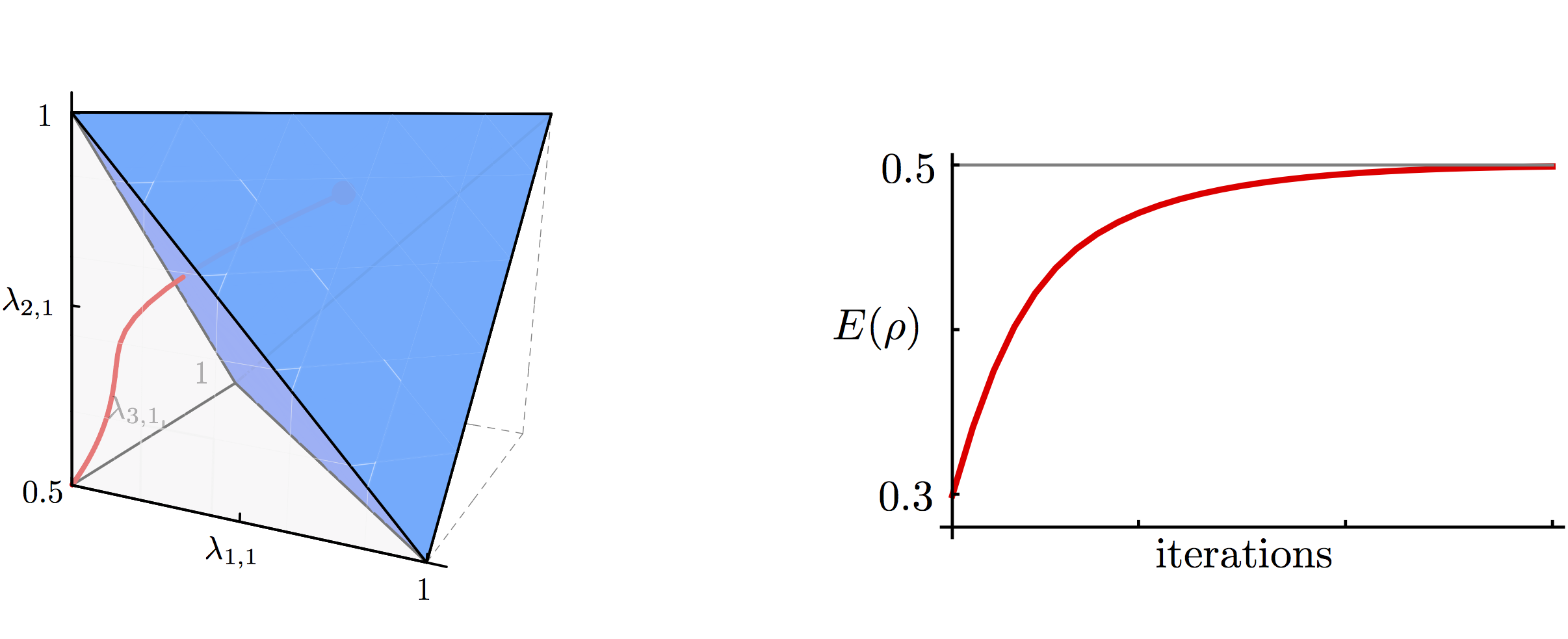
(a)

(b)

Figure 4.6: Illustration of entanglement distillation. (a) For the three-qubit quantum state $\rho=\lvert\psi\rangle\langle\psi\rvert$ from (4.6), the gradient flow (red trajectory) reaches the origin $O=(0.5,0.5,0.5)$ asymptotically. (b) The linear entropy of entanglement $E(\rho)$ increases monotonically until it reaches its maximal value.

Towards a Probabilistic Algorithm for Computing Moment Polytopes of Orbit Closures

From a theoretical perspective, the limit point $\rho_{\infty}$ of the gradient flow can also be seen as a normal form of the state $\rho$ in its entanglement class, as it is unique up to local unitaries. This is the point of view taken in [VDDM03], where a similar algorithm has been proposed for the case when the entanglement polytope contains the origin. In contrast, the gradient flow works in the general case and flows towards the point in the moment polytope of minimal Euclidean norm. We will now sketch how this idea leads towards a probabilistic algorithm for computing moment polytopes of arbitrary orbit closures. As above, let $\lVert-\rVert$ denote the norm corresponding to a $K$-invariant inner product $(-,-)$ on $i\mathfrak{k}^{*}$. We start with a simple observation:

Lemma .

Let $\lambda,\mu\in i\mathfrak{t}^{*}_{+}$. Then:

$$\min_{\varphi\in\mathcal{O}_{K,\mu}}\lVert\varphi-\lambda\rVert^{2}=\lVert\mu-\lambda\rVert^{2}$$

Proof.

By $K$-invariance of the inner product,

$$\min_{\varphi\in\mathcal{O}_{K,\mu}}\lVert\varphi-\lambda\rVert^{2}=\lVert\mu\rVert^{2}+\lVert\lambda\rVert^{2}-2\max_{\varphi\in\mathcal{O}_{K,\mu}}(\varphi,\lambda)$$

The right-hand side maximization can be understood as an optimization of the linear functional $(-,\lambda)$ over the Abelian moment polytope of the coadjoint orbit $\mathcal{O}_{K,\mu}$. By Kostant’s convexity theorem [Kos73], the latter is equal to the convex hull of the orbit of $\mu$ under the Weyl group, which in turn is a subset of $\mu$ plus the cone spanned by the negative roots. We conclude that

$$\max_{\varphi\in\mathcal{O}_{K,\mu}}(\varphi,\lambda)=\max_{w\in W_{K}}(w\mu,\lambda)=(\mu,\lambda).\qed$$

Now let $\mathbbm{X}=\overline{G\cdot\rho}\subseteq\mathbbm{P}(\mathcal{H})$ be an orbit closure. As in the proof of Section 2.2, fix $\lambda\in\Lambda^{*}_{+}$ and $k>0$. Let $\widetilde{\mathcal{H}}:=\operatorname{Sym}^{k}(\mathcal{H})\otimes V_{G,\lambda^{*}}$ and consider the projective subvariety $\widetilde{\mathbbm{X}}:=\{\lvert\psi\rangle\langle\psi\rvert^{\otimes k}\otimes\lvert\phi\rangle\langle\phi\rvert:\lvert\psi\rangle\langle\psi\rvert\in\mathbbm{X},\lvert\phi\rangle\langle\phi\rvert\in\mathbbm{X}_{G,\lambda^{*}}\}$ of $\mathbbm{P}(\widetilde{\mathcal{H}})$. As a set, $\widetilde{\mathbbm{X}}$ can be identified with the Cartesian product $\mathbbm{X}\times\mathcal{O}_{K,\lambda^{*}}$ equipped with the diagonal $K$-action Section 2.2), and the moment map $\widetilde{\mu}_{K}$ takes the form $\widetilde{\mu}_{K}(\rho,\varphi)=k\,\mu_{K}(\rho)+\varphi$. The following lemma is another instance of the “shifting trick” we used in the proof of Section 2.2.

Lemma .

Let $(\sigma,\varphi)\in\mathbbm{X}\times\mathcal{O}_{K,\lambda^{*}}\cong\widetilde{\mathbbm{X}}$ be such that $\widetilde{\mu}_{K}(\sigma,\varphi)$ is a point of minimal norm in $\widetilde{\mu}(\widetilde{\mathbbm{X}})$. If $\mu_{K}(\sigma)\in i\mathfrak{t}^{*}_{+}$ then it is the point of minimal distance to $\lambda/k$ in $\Delta_{K}(\mathbbm{X})$.

Proof.

By assumption and using that $\mathcal{O}_{K,\lambda^{*}}=-\mathcal{O}_{K,\lambda}$,

$$\lVert\mu_{K}(\sigma)+\varphi/k\rVert=\min_{\varphi^{\prime}\in\mathcal{O}_{K,\lambda^{*}}}\lVert\mu_{K}(\sigma)+\varphi^{\prime}/k\rVert=\min_{\varphi^{\prime}\in\mathcal{O}_{K,\lambda}}\lVert\mu_{K}(\sigma)-\varphi^{\prime}/k\rVert=\lVert\mu_{K}(\sigma)-\lambda/k\rVert,$$

where the last equality is due to Section 4.5. On the other hand,

$$\lVert\mu_{K}(\sigma)+\varphi/k\rVert= \min_{\sigma^{\prime}\in\mathbbm{X},\varphi^{\prime}\in\mathcal{O}_{K,\lambda^{*}}}\lVert\mu_{K}(\sigma^{\prime})+\varphi^{\prime}/k\rVert=\min_{\sigma^{\prime}\in\mathbbm{X},\varphi^{\prime}\in\mathcal{O}_{K,\lambda}}\lVert\mu_{K}(\sigma^{\prime})-\varphi^{\prime}/k\rVert$$

$$= \min_{\sigma^{\prime}\in\mathbbm{X}}\lVert\mu_{K}(\sigma^{\prime})-\lambda/k\rVert=\min_{\mu\in\Delta_{K}(\mathbbm{X})}\lVert\mu-\lambda/k\rVert.$$

The third equality is due to the $K$-invariance of the norm; for the last equality we have used Section 4.5 once more, but this time applied to the coadjoint orbit through the optimal $\mu_{K}(\sigma^{\prime})$. Since the convex polytope $\Delta_{K}(\mathbbm{X})$ contains a unique point of minimal Euclidean distance to $\lambda/k$, this point ought to be $\mu_{K}(\sigma)\in\Delta_{K}(\mathbbm{X})$. ∎

Note that $\widetilde{\mathbbm{X}}$ is not an orbit closure. However, just as we found in Section 4.3 for projective space, the moment polytope of the orbit closure of a generic point in $\widetilde{\mathbbm{X}}$ is always equal to the moment polytope $\Delta_{K}(\widetilde{\mathbbm{X}})$ [Bri87]. Since the “boundary” $(\mathbbm{X}\setminus G\cdot\rho)\times\mathcal{O}_{K,\lambda^{*}}$ is of positive codimension in $\widetilde{\mathbbm{X}}$ and by $G$-equivariance, we may in fact start with a point of the form $(\rho,\operatorname{Ad}^{*}(g)\lambda^{*})$. If we choose $g\in K$ according to, e.g., the Haar measure on $K$ then with probability one the gradient flow will asymptotically reach the point of minimal Euclidean norm in the moment polytope of $\widetilde{\mathbbm{X}}$. In view of Section 4.5 we thus obtain a “probabilistic oracle” for obtaining from any $\nu=\lambda/k\in\mathbbm{Q}\Lambda^{*}_{+}$ an approximation to the point $\mu\in\Delta_{K}(\mathbbm{X})$ that is closest to $\nu$. Note that $\mu$ is always rational if the inner product takes rational values on the integral lattice [Kir84a]. Let us assume for simplicity that the oracle does in fact never fail and always returns the exact result. Then we obtain the following algorithm:

Algorithm .

Let $\mathcal{H}$ be a complex $G$-representation and $\mathbbm{X}=\overline{G\cdot\rho}\subseteq\mathbbm{P}(\mathcal{H})$ an orbit closure. Let $\mathcal{V},\mathcal{W}\subseteq\mathbbm{Q}\Lambda^{*}_{+}$ be the vertices of an inner and an outer approximation of the moment polytope, i.e.,

$$\operatorname{conv}\mathcal{V}\subseteq\Delta_{K}(\mathbbm{X})\subseteq\operatorname{conv}\mathcal{W}.$$ (4.16)

The following algorithm returns the moment polytope of the orbit closure (if it terminates):

while $\mathcal{V}\subsetneq\mathcal{W}$ do

     $\nu\leftarrow\mathcal{W}\setminus\mathcal{V}$.

     $\mu\leftarrow$ the closest point in $\Delta_{K}(\mathbbm{X})$ to $\nu$ $\triangleright$ Oracle

     if $\mu=\nu$ then

         $\mathcal{V}\leftarrow$ vertices of $\operatorname{conv}\left(\mathcal{V}\cup\{\nu\}\right)$

     else

         $\mathcal{W}\leftarrow$ vertices of $\operatorname{conv}(\mathcal{W})\cap\{\lambda\in i\mathfrak{t}^{*}:(\lambda-\mu,\nu-\mu)\leq 0\}$

     end if

end while

return $\operatorname{conv}\mathcal{V}=\operatorname{conv}\mathcal{W}$

Proof.

To show that the algorithm is correct it suffices to observe that (4.16) is a loop invariant. In the case $\mu=\nu$ this is immediate. If $\mu\neq\nu$ then the convexity of the moment polytope implies that it is contained in the half-space $\{\lambda\in i\mathfrak{t}^{*}:(\lambda-\mu,\nu-\mu)\leq 0\}$. ∎

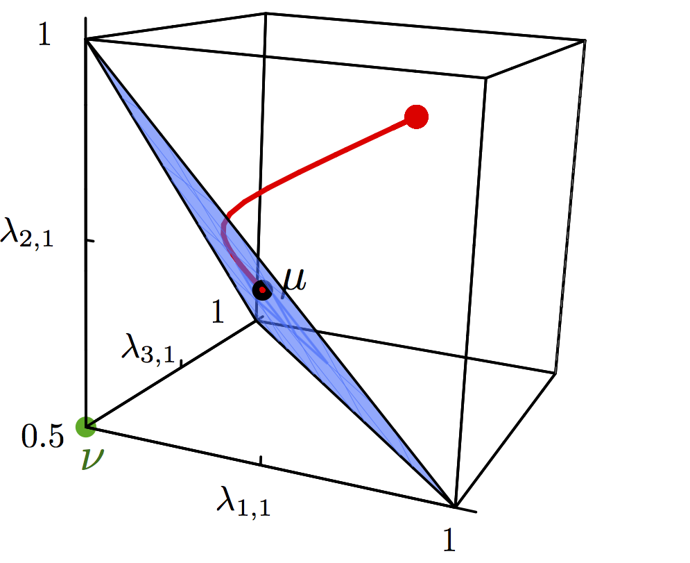
Figure 4.7: Illustration of Section 4.5 for a state $\rho$ of W class. In the first step, the gradient flow tries to flow from the spectrum of $\rho$ (red point) to the origin $\nu=(0.5,0.5,0.5)$ (green point), which is a vertex of the initial outer approximation (cube). The gradient flow stops at $\mu=(2/3,2/3,2/3)$, which is the closest point to $\nu$ in the entanglement polytope of $\rho$. We thus obtain a bounding hyperplane (blue) which gives rise to a smaller outer approximation. By iterating this procedure we will eventually recover the polytope of the W class (Figure 4.3, (b)).

One choice of outer approximation is given by the moment polytope for the action of the maximal torus $T\subseteq K$, which is equal to the convex hull of the weights of the representation $\mathcal{H}$ (Section 3.2). See Figure 4.7 for an illustration of the algorithm. Section 4.5, its theoretical properties and implications still need be investigated more carefully; we refer to [Wer13] for an initial study and first applications of the algorithm to the computation of entanglement polytopes. We remark that it can also be used to obtain a solution of the one-body quantum marginal problem when applied to a generic state $\rho$ (chosen, e.g., according to the unitarily invariant measure on projective space). We remark that the gradient flow gives us in essence a separation oracle [GLS93]. There are geometric algorithms that work with a separation oracle, e.g., based on the ellipsoid method, which are well-studied in the optimization community (as was kindly pointed out to us by Peter Bürgisser). A combination of these techniques might lead to further progress towards solving the membership problem for moment polytopes.

4.6 Experimental Noise

A quantum state prepared in the laboratory will always be a mixed state $\rho$ and it is a priori unclear what statements can be inferred about its entanglement from its local eigenvalues. Here, we give two slightly different ways for applying the preceding results to the more realistic scenario of small noise.

For both approaches, we will assume that a lower bound $p>1/2$ on the purity $\operatorname{tr}\rho^{2}$ is available. One natural way of obtaining such an estimate is the well-known swap test [BCWdW01], which directly estimates $\operatorname{tr}\rho^{2}$ using a series of two-body measurements on two copies of $\rho$. We sketch an alternative procedure which may be simpler to implement for some experimental platforms. Suppose that $\rho$ has been prepared by acting on an initial product state with a quantum operation $\Lambda$ that approximates an entangling unitary gate $U$ (e.g., a spin squeezing operation). Act on $\rho$ by a quantum operation $\Lambda^{\prime}$ that approximates the corresponding “disentangling unitary” $U^{-1}$ and denote by $\rho^{\prime}=\Lambda^{\prime}(\rho)$ the state thus obtained. Now assume that the noise mechanism never increases the purity—this holds, e.g., for dephasing and depolarizing noise, which are two noise models applicable to the majority of experiments. Then we can use the following lower bound [Aud07]

$$\operatorname{tr}\rho^{2}\geq\operatorname{tr}(\rho^{\prime})^{2}\geq\sum_{k=1}^{n}\lVert\vec{\lambda^{\prime}_{k}}\rVert^{2}_{2}-(n-1)$$

for the purity in terms of the local spectra $\vec{\lambda^{\prime}_{1}},\dots,\vec{\lambda^{\prime}_{n}}$, which can be obtained from tomography of the single-particle reduced density matrices $\rho^{\prime}_{1},\dots,\rho^{\prime}_{n}$. For small noise, $\rho^{\prime}$ is still approximately product and so this bound likely not too loose (as it is tight for product states).

Fidelity

The first way of dealing with noise is to realize that in the vicinity of any mixed state $\rho$ there is a pure state whose local eigenvalues do not differ too much from those of the mixed state, provided that the purity of the mixed state is sufficiently high. To make this precise, it is convenient to consider the fidelity between $\rho$ and an arbitrary pure state $\sigma=\lvert\psi\rangle\langle\psi\rvert$, which is defined by $F(\rho,\sigma):=\braket{\psi}{\rho}{\psi}$. Note that $F(\rho,\sigma)\leq 1$, with equality if and only if $\rho=\sigma$.

Proposition .

Let $\rho$ be a mixed state with purity $\operatorname{tr}\rho^{2}\geq p>1/2$. Then there exists a pure state $\sigma=\lvert\psi\rangle\langle\psi\rvert$ with fidelity $F(\rho,\sigma)\geq p$ such that

$$\sum_{k=1}^{n}\lVert\vec{\lambda}_{k}(\rho)-\vec{\lambda}_{k}(\sigma)\rVert_{1}\leq n(1-\sqrt{2p-1}),$$ (4.17)

where $\vec{\lambda}_{k}(\rho):=\operatorname{spec}\rho_{k}$ and where $\lVert x\rVert_{1}:=\sum_{j}\lvert x_{j}\rvert$ denotes the $\ell_{1}$-norm.

Proof.

Consider the spectral decomposition $\rho=\sum_{i}r_{i}\lvert\psi_{i}\rangle\langle\psi_{i}\rvert$ with eigenvalues ordered non-increasingly, $r_{i}\geq r_{i+1}$. Our assumption on the purity implies immediately that the maximal eigenvalue can also be lower-bounded by $1/2$:

$$r_{1}=r_{1}\sum_{i}r_{i}\geq\sum_{i}r_{i}^{2}=\operatorname{tr}\rho^{2}\geq p>\frac{1}{2}$$ (4.18)

Thus if we set $\sigma=\lvert\psi_{1}\rangle\langle\psi_{1}\rvert$ then $F(\rho,\sigma)=\braket{\psi_{1}}{\rho}{\psi_{1}}=r_{1}\geq p$.

On the other hand, using that $r_{j}\leq\sum_{i>1}r_{i}=1-r_{1}$ for all $j>1$, we find that

$$p\leq\operatorname{tr}\rho^{2}=r_{1}^{2}+\sum_{j>1}r_{j}^{2}\leq r_{1}^{2}+(1-r_{1})^{2}=1-2r_{1}(1-r_{1}).$$

We solve this quadratic relation and obtain two possible solutions,

$$r_{1}\leq\frac{1}{2}\left(1-\sqrt{2p-1}\right)\quad\text{and}\quad r_{1}\geq\frac{1}{2}\left(1+\sqrt{2p-1}\right).$$

Only the right-hand side solution is compatible with $r_{1}>1/2$. By using Weyl’s perturbation theorem relating the $\ell^{1}$-norm distance of eigenvalues with the trace-norm distance of the corresponding operators [NC04, (11.46)] we thus obtain that

$$\sum_{k=1}^{n}\lVert\vec{\lambda}_{k}(\rho)-\vec{\lambda}_{k}(\sigma)\rVert_{1}\leq\sum_{k=1}^{n}\lVert\rho_{k}-\sigma_{k}\rVert_{1}$$ (4.19)

$$\leq\; n\lVert\rho-\lvert\psi_{1}\rangle\langle\psi_{1}\rvert\rVert_{1}=2n(1-r_{1})\leq n\left(1-\sqrt{2p-1}\right).$$ (4.20)

∎

In the case of qubits, the bound (4.17) can be equivalently written in terms of the maximal local eigenvalues,

$$\sum_{k=1}^{n}\lvert\lambda_{k,1}(\rho)-\lambda_{k,1}(\sigma)\rvert\leq\frac{n}{2}(1-\sqrt{2p-1}).$$ (4.21)

For small noise, the right-hand side is equal to $n\varepsilon/2$ in first order in $\varepsilon=1-p\approx 0$.

We now illustrate the approach with a numerical example. Suppose that $\rho$ is an experimentally prepared quantum state of four qubits with purity no less than $p=0.9$. Then by Section 4.6 above there exists a pure state $\sigma=\lvert\psi\rangle\langle\psi\rvert$ with fidelity $F(\rho,\sigma)\geq 0.9$ for which (4.21) reads

$$\sum_{k=1}^{4}\lvert\lambda_{k,1}(\rho)-\lambda_{k,1}(\sigma)\rvert\leq\frac{4}{2}\left(1-\sqrt{2p-1}\right)\approx 0.21.$$ (4.22)

At this resolution, the differences between the various four-qubit entanglement polytopes are already well visible. For example, suppose that we would like to use the inequality

$$\lambda_{1,1}(\sigma)+\lambda_{2,1}(\sigma)+\lambda_{3,1}(\sigma)+\lambda_{4,1}(\sigma)<3$$

to deduce that $\sigma$ is not entangled of W-type (cf. the summary of results in this chapter). For this, it suffices by (4.22) to verify that the local eigenvalues of the experimentally realized state $\rho$ satisfy the relation

$$\lambda_{1,1}(\rho)+\lambda_{2,1}(\rho)+\lambda_{3,1}(\rho)+\lambda_{4,1}(\rho)<3-0.21=2.79.$$

For comparison, the left-hand side of this inequality is equal to $2$ for a symmetric Dicke state $\left(\ket{0011}+\ket{0101}+\ket{0110}+\ket{1001}+\ket{1010}+\ket{1100}\right)/\sqrt{6}$.

Convex Extension

A second, alternative approach for treating noise aims to show that the experimentally prepared mixed state $\rho$ cannot be written as a convex combination of pure states in the closure of an entanglement class $\mathcal{X}$. For this, we consider the distance between a spectrum $\vec{\lambda}$ and an entanglement polytope $\Delta_{\mathcal{X}}$ defined as

$$d(\vec{\lambda},\Delta_{\mathcal{X}}):=\min_{\vec{\mu}\in\Delta_{\mathcal{X}}}\sum_{k=1}^{n}\lVert\vec{\lambda}-\vec{\mu}\rVert_{1}.$$

Proposition .

There exists a continuous function $\delta(p)\geq 0$ with $\delta(1)=0$ such that

$$d(\vec{\lambda}(\rho),\Delta_{\mathcal{X}})>\delta(p)\,\Longrightarrow\,\rho\not\in\operatorname{conv}\overline{\mathcal{X}}$$

for all mixed states $\rho$ with purity $\operatorname{tr}\rho^{2}\geq p>1/2$.

Proof.

Let $\delta(p):=n(1+2\sqrt{1-p}-\sqrt{2p-1})$. Then $\delta$ is continuous and non-negative on $[1/2,1]$, and $\delta(1)=0$. Now assume that $\rho$ is a mixed state with purity $\operatorname{tr}\rho^{2}\geq p>1/2$ and $d(\vec{\lambda}(\rho),\Delta_{\mathcal{X}})>\delta(p)$. As in the proof of Section 4.6, let $\sigma=\lvert\psi_{1}\rangle\langle\psi_{1}\rvert$ where $\ket{\psi_{1}}$ is an eigenvector corresponding to the maximal eigenvalue of $\rho$. For any $\chi=\lvert\phi\rangle\langle\phi\rvert\in\overline{\mathcal{X}}$, the triangle inequality gives

$$\lVert\chi-\sigma\rVert_{1}\geq\lVert\chi-\rho\rVert_{1}-\lVert\rho-\sigma\rVert_{1}.$$

We may lower-bound the first summand by reversing the argument of (4.19) and using the assumption on $\rho$,

$$\lVert\chi-\rho\rVert_{1}\geq\frac{1}{n}\sum_{k=1}^{n}\lVert\chi_{k}-\rho_{k}\rVert_{1}\geq\frac{1}{n}\sum_{k=1}^{n}\lVert\vec{\lambda}_{k}(\chi)-\vec{\lambda}_{k}(\rho)\rVert_{1}\geq\frac{d(\vec{\lambda}(\rho),\Delta_{\mathcal{X}})}{n}>\frac{\delta(p)}{n},$$

while the second summand can be upper-bounded as in (4.20),

$$\lVert\rho-\sigma\rVert_{1}=\lVert\rho-\lvert\psi_{1}\rangle\langle\psi_{1}\rvert\rVert_{1}\leq\left(1-\sqrt{2p-1}\right).$$

Together this implies

$$\lVert\chi-\sigma\rVert_{1}>\frac{\delta(p)}{n}-\left(1-\sqrt{2p-1}\right)=2\sqrt{1-p},$$

so that by using a standard upper bound for the fidelity in terms of the trace norm [FvdG99] we obtain the following estimate which holds for all $\chi=\lvert\phi\rangle\langle\phi\rvert\in\overline{\mathcal{X}}$:

$$\lvert\braket{\psi_{1}}{\phi}\rvert^{2}\leq 1-\frac{\lVert\chi-\sigma\rVert_{1}^{2}}{4}<p.$$

Now assume for the sake of reaching a contradiction that $\rho$ can in fact be written as a convex combination $\rho=\sum_{j}p_{j}\lvert\phi_{j}\rangle\langle\phi_{j}\rvert$ of pure states from $\overline{\mathcal{X}}$. Then,

$$\braket{\psi_{1}}{\rho}{\psi_{1}}=\sum_{j}p_{j}\lvert\braket{\psi_{1}}{\phi_{j}}\rvert^{2}<p.$$

But on the other hand, $\braket{\psi_{1}}{\rho}{\psi_{1}}\geq p$ by (4.18), which is the desired contradiction. ∎

4.7 Discussion

Section 4.3 provides a complete description of the entanglement polytopes based on a generating set of covariants. While the latter can in principle be found using computational invariant theory, current algorithms based on Gröbner bases work best for low-dimensional scenarios. It would therefore be highly desirable to find an alternative characterization that does not rely on an explicit knowledge of the covariants—for example, based on the differential-geometric approach of Chapter 3 or by using semistability computations in geometric invariant theory. The fact that only the vanishing behavior of the covariants enters the description in Section 4.3 indicates that such a characterization could indeed be achievable.

While the distillation method in Section 4.5 is conceptually pleasing, it is not clear when its realization will become experimentally feasible. In contrast, Section 4.5 has already been successfully implemented and might provide a way of circumventing the combinatorial challenges faced by exact methods in higher dimensions. Apart from its immediate applications to the marginal problem and entanglement witnessing, the computation of moment polytopes is also relevant in other disciplines such as in mathematics and in geometric complexity theory [BLMW11] (cf. Chapter 6), and it might be worthwhile to study our algorithm in this context.

Chapter 5 Random Marginals

In this chapter we consider a quantitative version of the one-body quantum marginal problem. For a random pure state drawn from the unitarily invariant measure, we give an algorithm to compute the joint probability distribution of the eigenvalues of its one-body reduced density matrices. We obtain the exact probability distribution by reducing to the corresponding distribution of diagonal entries, which corresponds to a quantitative version of a classical marginal problem. This reduction is an instance of a more general principle that can be used to compute Duistermaat–Heckman measures in symplectic geometry.

The results in this chapter have been obtained in collaboration with Matthias Christandl, Brent Doran and Stavros Kousidis, and they have appeared in [CDKW14].

5.1 Summary of Results

Let $\rho$ be a pure quantum state of $n$ particles, drawn at random according to the unitarily invariant probability measure on projective space. We consider the problem of determining the joint distribution of its one-body reduced density matrices $\rho_{1},\dots,\rho_{n}$, which are again random variables. This is a quantitative version of the one-body quantum marginal problem, Chapter 2, and strictly generalizes the latter – for a given collection of density matrices, we ask how likely it is to obtain them as the one-body marginals of a pure state rather than whether this is possible at all.

The starting point for our work is the observation that the joint distribution of the one-body reduced density matrices is invariant under the action of the local unitary group. In particular, this implies that we may equivalently consider the joint distribution of their eigenvalues, $\mathbf{P}_{\operatorname{spec}}$, which is a probability measure on the positive Weyl chamber $i\mathfrak{t}^{*}_{\geq 0}$ with support equal to the moment polytope (i.e., the solution to the one-body quantum marginal problem). The crucial fact is that in general $\mathbf{P}_{\operatorname{spec}}$ can be recovered from the corresponding distribution of local diagonal entries $\mathbf{P}_{\operatorname{diag}}$ by taking a number of partial derivatives:

$$\mathbf{P}_{\operatorname{spec}}=p(\vec{\lambda}_{1},\dots,\vec{\lambda}_{n})\prod_{k=1}^{n}\prod_{i<j}^{d_{k}}\left(\partial_{\lambda_{k,j}}-\partial_{\lambda_{k,i}}\right)\mathbf{P}_{\operatorname{diag}}\big{|}_{i\mathfrak{t}^{*}_{>0}},$$ (5.1)

where $d_{1},\dots,d_{k}$ are the local dimensions and where $p$ is an explicitly given polynomial (namely, a product of Vandermonde determinants). This is an instance of a more general derivative principle that relates invariant measures for the coadjoint action of a compact Lie group to their projections onto a Cartan subalgebra, and follows from a result by Harish-Chandra [HC57] (Section 5.4). A similar reduction is not possible on the level of the moment polytopes. To compute the distribution of diagonal entries, we show in Section 5.3 that its density $f_{\operatorname{diag}}$ can be written as the push-forward of Lebesgue measure on a simplex along a linear map. Concretely:

$$f_{\operatorname{diag}}(\vec{\lambda}_{1},\dots,\vec{\lambda}_{n})=\operatorname{vol}\{(p_{i_{1},\dots,i_{n}})\in\mathbbm{R}^{d_{1}\dotsm d_{n}}_{\geq 0}:\sum_{\mathclap{i_{1},\dots,i_{n}}}p_{i_{1},\dots,i_{n}}=1,$$ (5.2)

$$\sum_{\mathclap{i_{2},\dots,i_{n}}}p_{i_{1},\dots,i_{n}}=\vec{\lambda}_{1,i_{1}}\;(\forall i_{1}),\dots,\sum_{\mathclap{i_{1},\dots,i_{n-1}}}p_{i_{1},\dots,i_{n}}=\vec{\lambda}_{n,i_{n}}\;(\forall i_{n})\}$$

It is amusing to note that this corresponds precisely to a quantitative marginal problem for ordinary random variables. Any measure of the form (5.2) is given by piecewise homogeneous polynomials on convex chambers that can be explicitly computed. To do so algorithmically, we adapt a result of Boysal and Vergne that can be used to recursively compute closely related measures by evaluating residues [BV09]. By putting together all ingredients, we obtain an effective algorithm for computing $\mathbf{P}_{\operatorname{spec}}$ for an arbitrary number of particles and statistics (Section 5.4). See Figure 5.1 for a summary of the method. This generalizes previous results in the literature significantly, where exact results were only obtained for two distinguishable particles [LP88, ZS01]. In [CDKW14] we also give a variant of the algorithm that can be directly applied to non-pure global spectrum (while the general case can always be reduced to the case of random pure states, such an algorithm can be useful for the manual computation of concrete examples).

From a mathematical perspective, the distributions that we compute are Duistermaat–Heckman measures, which are defined more generally using the push-forward of the Liouville measure on a symplectic manifold along the moment map [Hec82, GS82b, GS84b, GLS88, GLS96, GP90] (Section 5.2). For the purposes of this thesis, it will be convenient to restrict our attention to projective space; we refer to [CDKW14] for an exposition from the symplectic point of view.

Figure 5.1: Illustration of the method. A random pure state $\rho$ gives rise to random one-body reduced density matrices $\rho_{1},\dots,\rho_{n}$. The derivative principle (5.1) allows their distribution of eigenvalues $\mathbf{P}_{\operatorname{spec}}$ to be recovered from the distribution of diagonal entries $\mathbf{P}_{\operatorname{diag}}$, which we compute algorithmically.

5.2 Duistermaat–Heckman Measures

We use the same notation and conventions as in Chapter 2. Thus let $G$ be a connected reductive algebraic group, $K\subseteq G$ a maximal compact subgroup, and $\Pi\colon G\rightarrow\operatorname{GL}(\mathcal{H})$ be a representation on a Hilbert space $\mathcal{H}$ with $K$-invariant inner product. Throughout this chapter we will assume that the moment polytope $\Delta_{K}:=\Delta_{K}(\mathbbm{P}(\mathcal{H}))$ has non-empty intersection with the interior of the positive Weyl chamber, $\Delta_{K}\cap i\mathfrak{t}^{*}_{>0}\neq\emptyset$. We explain below that this is without loss of generality for our application to eigenvalue distributions.

Let $\rho$ be a random pure state in $\mathbbm{P}(\mathcal{H})$, chosen according to the $\operatorname{U}(\mathcal{H})$-invariant probability measure on projective space. Then $\mu_{K}(\rho)$ is contained in a unique coadjoint orbit $\mathcal{O}_{K,\lambda}$, where $\lambda$ is a now random variable which takes values in the moment polytope $\Delta_{K}$. We call the distribution of $\lambda$ the non-Abelian Duistermaat–Heckman probability measure and denote it by $\mathbf{P}_{K}=\mathbf{P}_{K,\mathbbm{P}(\mathcal{H})}$. In other words, $\mathbf{P}_{K}$ is defined as the push-forward of the invariant measure on projective space first along the moment map and then along the continuous map that sends $\mathcal{O}_{K,\lambda}\mapsto\lambda$. Likewise, we may also consider the image of $\rho$ under the moment map (3.4) for the maximal torus $T\subseteq K$. Then $\mu_{T}(\rho)$ is a random variable that takes values in the “Abelian” moment polytope $\Delta_{T}$, which we have seen is just the convex hull of weights. We call the distribution of $\mu_{T}(\rho)$ the Abelian Duistermaat–Heckman probability measure and denote it by $\mathbf{P}_{T}=\mathbf{P}_{T,\mathbbm{P}(\mathcal{H})}$.

More generally, we may consider a random quantum state $\rho$ of fixed spectrum $\mu$ and consider the corresponding Duistermaat–Heckman measures $\mathbf{P}_{K,\mu}$ and $\mathbf{P}_{T,\mu}$ constructed in the same way as before. We will see in (5.6) below that the computation of these measures can always be reduced to the case of random pure states.

We remark that there is a general definition of a Duistermaat–Heckman measure in symplectic geometry that goes as follows: Let $(M,\omega)$ be a Hamiltonian $K$-manifold of dimension $2n$ and $\mu_{K}\colon M\rightarrow i\mathfrak{k}^{*}$ its moment map. Then $\omega^{n}/(2\pi)^{n}n!$ is a volume form on $M$ that determines the Liouville measure of $M$. By pushing forwarding along the moment map $\mu_{K}$ and further along the map $\mathcal{O}_{K,\lambda}\mapsto\lambda$ we obtain the Duistermaat–Heckman measure for the $K$-action on $M$. If $M$ is compact then we can renormalize to obtain a probability measure $\mathbf{P}_{K,M}$ on the moment polytope. We remark that in our definition of the non-Abelian Duistermaat–Heckman measure in [CDKW14] we had furthermore divided the push-forward measure at each point by the Liouville volume of the respective coadjoint orbit, given by

$$p_{K}(\lambda)=\prod_{\alpha\in R_{K,+}}\frac{(\lambda,H_{\alpha})}{(\rho_{K},H_{\alpha})}$$ (5.3)

where $\rho_{K}=\frac{1}{2}\sum_{\alpha\in R_{K,+}}\alpha$ is the Weyl vector [BGV03, Proposition 7.26]. This is conceptually more appealing since it corresponds to “intersecting” with the positive Weyl chamber – just as in the definition of the moment polytope! – and it makes the formulas slightly cleaner. However, it comes at the expense of working with measures that are not probability measures, and we have chosen not to adopt this convention herein.

Eigenvalues and Diagonal Entries

Let us now consider the groups and representations that correspond to the one-body quantum marginal problem and its variants (cf. Table 2.3). In the case of distinguishable particles, $G=\operatorname{SL}(\mathcal{H}_{1})\times\dots\times\operatorname{SL}(\mathcal{H}_{n})$, $K=\operatorname{SU}(\mathcal{H}_{1})\times\dots\times\operatorname{SU}(\mathcal{H}_{n})$, and $\mathcal{H}=\mathcal{H}_{1}\otimes\dots\otimes\mathcal{H}_{n}$. As in the preceding chapters, we may identify the collection of local eigenvalues with points in the positive Weyl chamber $i\mathfrak{t}^{*}_{+}$; likewise, the collection of local diagonal entries can be identified with points in $i\mathfrak{t}^{*}$ (Section 2.3). In this way, the eigenvalue distribution $\mathbf{P}_{\operatorname{spec}}$ and the distribution of local diagonal entries $\mathbf{P}_{\operatorname{diag}}$ introduced in Section 5.1 are identified with the Duistermaat–Heckman probability measures $\mathbf{P}_{K}$ and $\mathbf{P}_{T}$, respectively.

For two distinguishable particles, $\mathcal{H}=\mathbbm{C}^{d}\otimes\mathbbm{C}^{d}$, the solution is well-known [LP88, ZS01]:

$$\int d\mathbf{P}_{\operatorname{spec}}\,f=\frac{1}{Z}\int_{\Delta_{d,+}}d\vec{\lambda}_{A}\;p^{2}_{d}(\vec{\lambda}_{A})\,f(\vec{\lambda}_{A},\vec{\lambda}_{A})$$ (5.4)

for any test function $f=f(\vec{\lambda}_{A},\vec{\lambda}_{B})$. Here,

$$\Delta_{d,+}=\{\vec{\lambda}\in\mathbbm{R}^{d}_{\geq 0}:\sum_{j}\lambda_{j}=1,\,\lambda_{1}\geq\dots\geq\lambda_{d}\}$$

denotes the non-increasingly ordered chamber in the $(d-1)$-dimensional standard simplex, which can be identified with the set of possible spectra of a density operators on $\mathbbm{C}^{d}$;

$$p_{d}(\vec{\lambda})=\prod_{i<j}\frac{\lambda_{i}-\lambda_{j}}{j-i}$$ (5.5)

is the volume polynomial (5.3) for $K=\operatorname{SU}(d)$, and $Z>0$ is a suitable normalization constant. Note that the measure $\mathbf{P}_{\operatorname{spec}}$ is supported on the “diagonal” $\vec{\lambda}_{A}=\vec{\lambda}_{B}$, in agreement with Chapter 2. We will later give a simple proof of (5.4) using the methods of this chapter (see (5.26)). The corresponding distribution of the one-body reduced density matrix $\rho_{A}$ is known as the Hilbert–Schmidt probability measure.

Just as Chapter 2 did for the one-body quantum marginal problem, its quantitative version (5.4) can be used to reduce the seemingly more general problem of computing the local eigenvalue distribution for random states with fixed global spectrum to the case of global pure states. More generally, let $\mathcal{H}_{0}$ be a $K_{0}$-representation (e.g., one from Table 2.3) and $\mathcal{H}=\mathcal{H}_{0}\otimes\mathcal{H}_{0}$ the corresponding representation of $K=K_{0}\times\operatorname{SU}(\mathcal{H}_{0})$ (its “purification”). Then (5.4) implies that the probability measure $P_{K}$ for pure states can be obtained as a direct integral of the measures $P_{K_{0},\mu}$ for fixed global spectrum $\mu$,

$$\int d\mathbf{P}_{K}\,f=\frac{1}{Z}\int_{\Delta_{d,+}}d\vec{\mu}\;p^{2}_{d}(\vec{\mu})\int d\mathbf{P}_{K_{0},\mu}(\vec{\lambda})\;f(\vec{\lambda},\vec{\mu}),$$ (5.6)

where $d=\dim\mathcal{H}_{0}$. Conversely, since the probability distributions $\mathbf{P}_{K_{0},\mu}$ vary continuously with the global spectrum $\mu$, they can be reconstructed from $\mathbf{P}_{K}$ by taking limits.

Our assumption that the moment polytope $\Delta_{K}$ has non-empty intersection with the interior of the positive Weyl chamber amounts to showing that there exists a global pure state $\rho$ whose reduced density matrices all have non-degenerate eigenvalue spectrum. We first give a criterion in the case of distinguishable particles:

Lemma .

Let $n\geq 1$ and $d_{1}\leq\dots\leq d_{n}\leq d_{n+1}$. Then there exists a global pure state $\rho$ on $\mathcal{H}=\mathbbm{C}^{d_{1}}\otimes\dots\otimes\mathbbm{C}^{d_{n+1}}$ such that $\rho_{1},\dots,\rho_{n+1}$ all have non-degenerate spectrum if and only if $d_{n+1}\leq\left(\prod_{k=1}^{n}d_{k}\right)+1.$

Proof.

The condition is clearly necessary, since it follows from Chapter 2 that at most $\prod_{k=1}^{n}d_{k}$ eigenvalues of $\rho_{n+1}$ are non-zero. To show that it is sufficient, consider the following mixed state on $\mathbbm{C}^{d_{1}}\otimes\dots\otimes\mathbbm{C}^{d_{n}}$,

$$\rho_{1,\dots,n}\propto\sum_{j=1}^{d_{n}}2^{-j}\lvert j\rangle\langle j\rvert_{1}\otimes\dots\otimes\lvert j\rangle\langle j\rvert_{n},$$

where we set $\lvert j\rangle\langle j\rvert_{k}:=\lvert d_{k}\rangle\langle d_{k}\rvert$ if $j>d_{k}$. It is not hard to see that each $\rho_{k}$ has non-degenerate spectrum. The same remains true if we perturb $\rho_{1,\dots,n}$ slightly such that it has non-degenerate global spectrum with all eigenvalues positive. Let $\rho$ denote a purification of $\rho_{1,\dots,n}$ on $\mathcal{H}$. Then Chapter 2 shows $\rho_{n+1}$ and therefore all one-body reduced density matrices of $\rho$ have non-degenerate spectrum. ∎

Note that the conditions of Section 5.2 are always satisfied for the purification, where $d_{n+1}=d_{1}\dotsm d_{n}$. The following lemma shows that the same is true for the one-body $n$-representability problem:

Lemma .

Let $d>n\geq 1$. Then there exists a mixed state $\rho$ on $\bigwedge^{n}\mathbbm{C}^{d}$ such that both $\rho$ and $\rho_{1}$ have non-degenerate spectrum.

Proof.

The weights of $\bigwedge^{n}\mathbbm{C}^{d}$ can be identified with fermionic occupation numbers, i.e., binary strings $\vec{\omega}\in\{0,1\}^{d}$ with precisely $n$ ones. As long as $1\leq n<d$, we can find $d$ linearly independent such weights. Thus their convex hull is maximal-dimensional and we can find a convex combination $\sum_{j}p_{j}\,\vec{\omega}_{j}\in i\mathfrak{t}^{*}_{>0}$. Then the one-body reduced density matrix $\rho_{1}$ of $\rho=\sum_{j}p_{j}\lvert\omega_{j}\rangle\langle\omega_{j}\rvert$ has non-degenerate spectrum, and by slightly perturbing $\rho$ we can arrange that the same is true for the global state. ∎

For bosons, we have already seen that any one-body reduced density matrix is consistent with a global pure state.

The Post-Selection Bound

We briefly digress to prove a useful property of the Hilbert–Schmidt probability measure that will be needed in Chapter 9. Let $P_{k,d}$ denote the projector onto the symmetric subspace $\operatorname{Sym}^{k}(\mathbbm{C}^{d})\subseteq(\mathbbm{C}^{d})^{\otimes k}$ and $d_{k,d}$ its dimension. Then we have that

$$\frac{P_{k,d}}{d_{k,d}}=\int_{\mathbbm{P}(\mathbbm{C}^{d})}d\rho\,\rho^{\otimes k},$$ (5.7)

where $d\rho$ the probability distribution of a random pure state on $\mathbbm{C}^{d}$. To see this, note that the right-hand side is an operator on the irreducible $\operatorname{U}(d)$-representation $\operatorname{Sym}^{k}(\mathbbm{C}^{d})$ that commutes with the group action, and therefore proportional to $P_{k,d}$ by Schur’s lemma (2.23). Thus (5.7) follows from the observation that both the left and the right-hand side have trace one.

Now let $\sigma_{A^{k}}$ be a permutation-invariant density operator on $(\mathbbm{C}^{a})^{\otimes k}$. Then there exists a purification $\sigma_{(AA^{\prime})^{k}}$ of $\sigma_{A^{k}}$ that is supported on the symmetric subspace $\operatorname{Sym}^{k}(\mathbbm{C}^{a}\otimes\mathbbm{C}^{a})\subseteq(\mathbbm{C}^{a}\otimes\mathbbm{C}^{a})^{\otimes k}=(\mathbbm{C}^{a})^{\otimes k}\otimes(\mathbbm{C}^{a})^{\otimes k}$ [CKMR07, Ren05]. Indeed, by Schur’s lemma, $\sigma_{A^{k}}$ is of the form $\bigoplus_{\alpha\vdash_{a}k}\sigma_{\alpha}\otimes\mathbbm{1}_{[\alpha]}/\!\dim[\alpha]$ with respect to the Schur–Weyl decomposition $\bigoplus_{\alpha\vdash_{a}k}V^{a}_{\alpha}\otimes[\alpha]$ (2.20). In view of (2.25), the desired purification can thus be constructed by purifying each part $\sigma_{\alpha}$. Together with (5.7) for $d=a^{2}$, we find that

$$\sigma_{(AA^{\prime})^{k}}\leq P_{k,a^{2}}=d_{k,a^{2}}\int_{\mathbbm{P}(\mathbbm{C}^{a}\otimes\mathbbm{C}^{a})}d\rho_{AA^{\prime}}\,\rho_{AA^{\prime}}^{\otimes k}.$$

where “$\leq$” denotes the positive semidefinite order of Hermitian matrices. Since the latter is preserved by the partial trace, we obtain the following bound, which holds for any permutation-invariant density operator $\sigma_{A^{k}}$:

$$\sigma_{A^{k}}\leq d_{k,a^{2}}\int d\rho_{A}\,\rho_{A}^{\otimes k},$$ (5.8)

where $d\rho_{A}$ is the Hilbert–Schmidt probability measure on the set of density matrices on $\mathbbm{C}^{a}$. It is a remarkably useful tool to lift permutation-invariance to tensor-product form at the expense of a factor $d_{k,a^{2}}=\binom{k+a^{2}-1}{k}$ which grows only polynomially with $k$ (for fixed local dimension $a$). A more refined version of this observation is known as the post-selection technique [CKR09, Ren10] (cf. [Hay10]).

5.3 The Abelian Measure

We now compute the Abelian Duistermaat–Heckman probability measure $\mathbf{P}_{T}$ for the projective space $\mathbbm{P}(\mathcal{H})$. Let $\Omega$ denote the set of weights of the representation $\mathcal{H}$. Choose an orthonormal basis $\ket{k}$ of weight vectors with corresponding weights $\omega_{k}\in\Omega$. According to (3.5), the image of a pure state $\rho=\lvert\psi\rangle\langle\psi\rvert$ with $\ket{\psi}=\sum_{k}\psi_{k}\ket{k}$ is given by the convex combination

$$\mu_{T}(\rho)=\sum_{k}\lvert\psi_{k}\rvert^{2}\omega_{k}.$$ (5.9)

Let

$$\Delta_{D}:=\{(p_{k})\in\mathbbm{R}^{D}_{\geq 0}:\sum_{k}p_{k}=1\}$$

denote the $(D-1)$-dimensional standard simplex, where $D=\dim\mathcal{H}$. In the following, a Lebesgue measure on a closed convex body is the restriction of a translation-invariant measure on its affine hull (such a measure is unique up to normalization).

Lemma .

The Abelian Duistermaat–Heckman probability measure $\mathbf{P}_{T}$ is equal to the push-forward of Lebesgue measure $dp$ on the standard simplex $\Delta_{D}$, normalized to probability one, along the linear map $\Phi\colon(p_{k})\mapsto\sum_{k}p_{k}\omega_{k}$.

Proof.

The invariant probability measure on $\mathbbm{P}(\mathcal{H})$ is the push-forward of the usual round measure on the unit sphere $S^{2D-1}\cong\{\ket{\psi}:\braket{\psi}{\psi}=1\}$, normalized to total measure one, along the quotient map $\ket{\psi}\mapsto\lvert\psi\rangle\langle\psi\rvert$. On the other hand, the round measure on the unit sphere also induces Lebesgue measure on the standard simplex $\Delta_{D}$ by pushing forward along the map $\ket{\psi}\mapsto(\lvert\psi_{k}\rvert^{2})$ (polar coordinates!). Thus the claim follows from (5.9). ∎

Now fix a Lebesgue measure $d\lambda$ on the affine hull of Abelian moment polytope $\Delta_{T}=\operatorname{conv}\Omega$. Away from the boundary of the standard simplex, the map $(p_{k})\mapsto\sum_{k}p_{k}\omega_{k}$ is a submersion onto this affine space, and therefore the measure $\mathbf{P}_{T}$ is absolutely continuous with respect to $d\lambda$. In fact, its density function $f_{T}(\lambda)$ is given by

$$f_{T}(\lambda)= \operatorname{vol}\leavevmode\nobreak\ (\Phi^{-1}(\lambda)\cap\Delta_{D})$$ (5.10)

$$= \operatorname{vol}\leavevmode\nobreak\ \{(p_{k})\in\mathbbm{R}^{D}_{\geq 0}:\sum_{k}p_{k}=1,\sum_{k}p_{k}\omega_{k}=\lambda\},$$

i.e., as the volume of a parametrized polytope, measured with respect to a Lebesgue measure $dp/d\lambda$ on the fiber $\Phi^{-1}(\lambda)\cap\Delta_{D}$ that is normalized such that $dp=dp/d\lambda\wedge d\lambda$ (we freely identify differential pseudo-forms and the measures induced by them). For the one-body quantum marginal problem, (5.10) reduces to (5.2), the quantitative version of a classical marginal problem that we discussed in the introduction.

In special case that $D-1=\dim\Delta_{T}$, the map $\Phi$ maps the standard simplex bijectively onto the Abelian moment polytope $\Delta_{T}$ (which in this case is itself a simplex). It follows that

$$\mathbf{P}_{T}=\frac{(D-1)!}{d\lambda(\omega_{2}-\omega_{1},\dots,\omega_{D}-\omega_{1})}d\lambda,$$ (5.11)

where the denominator denotes the volume of the parallelotope spanned by the $(\omega_{j}-\omega_{1})$ as measured by $d\lambda$. In particular, the Abelian Duistermaat–Heckman measure for the maximal torus of $\operatorname{U}(\mathcal{H})$ is simply Lebesgue probability measure on the standard simplex, which is in agreement with Section 5.3.

In the general case, $D-1>\dim\Delta_{T}$. Consider subsets of weights whose convex hull have codimension one in $\Delta_{T}$. These convex hulls are precisely the critical points of the Abelian moment map, viewed as a map onto the affine hull of $\Delta_{T}$ (the proof of Section 3.2 works just as well if $\Delta_{T}$ is of positive codimension). They cut $\Delta_{T}$ into convex polytopes that we will call the regular chambers. We will also considered the complement of $\Delta_{T}$ as a chamber, called the unbounded chamber, although it is not convex. If the closures of two chambers have a common boundary of maximal dimension (i.e., of codimension one) then we shall say that the two chambers are adjacent. The affine hyperplane spanned by their common boundary will be called a critical wall. The significance of these notions is the following: Inside each regular chamber, the vertices of the convex polytopes $\Phi^{-1}(\lambda)\cap\Delta_{D}$ can be parametrized as affine functions of $\lambda$ (see, e.g., [CL98, VSB⁺07] for details). It follows that the density function $f_{T}(\lambda)$ is given by a polynomial of degree at most $(D-1)-r_{T}$ on (the interior of) each regular chamber, where we set $r_{T}=\dim\Delta_{T}$. Thus we say that $f_{T}(\lambda)$ is a piecewise polynomial function. As we cross a critical wall, this polynomial will in general change, and we will now describe a way to compute these “jumps”.

The Boysal–Vergne–Paradan Jump Formula

In [BV09], Boysal and Vergne have analyzed the push-forward of Lebesgue measure on the cone $\mathbbm{R}^{D}_{\geq 0}$ along a linear map. In view of Section 5.3, such measures are closely related to the Abelian Duistermaat–Heckman measure $\mathbf{P}_{T}$, and it is straightforward to translate their [BV09, Theorem 4.3] into the projective scenario. We refer to [CDKW14] for a detailed derivation and only present the result:

Consider two adjacent chambers separated by a critical wall $(-,H)=c$. Let $\Omega_{0}:=\{\omega\in\Omega:(\omega,H)=c\}$ denote the set of weights on the wall, $\mathcal{H}_{0}=\bigoplus_{\omega\in\Omega_{0}}\mathcal{H}_{\omega}$ the corresponding sum of weight spaces, and $D_{0}:=\dim\mathcal{H}_{0}$ its dimension. Let $d\lambda_{0}$ be Lebesgue measure on the affine hyperplane $(-,H)=c$, normalized such that

$$d\lambda=d\lambda_{0}\wedge d(-,H).$$ (5.12)

The common boundary between the two chambers is contained in a single regular chamber for $\mathbbm{P}(\mathcal{H}_{0})$. Thus the Abelian Duistermaat–Heckman measure $\mathbf{P}_{T,\mathbbm{P}(\mathcal{H}_{0})}$ is there given by a polynomial density function with respect to $d\lambda_{0}$. Let $f_{T,0}(\lambda)$ denote any polynomial that extends this density to all of $i\mathfrak{t}^{*}$ and consider its “homogeneous extension” $F_{T,0}(\lambda,t):=t^{D_{0}-r_{T}}f_{T,0}(\lambda/t)$. Finally, let $f_{T,\pm}$ denote the polynomial density function of $\mathbf{P}_{T,\mathbbm{P}(\mathcal{H})}$ on the chamber on the positive and negative side of the critical wall, respectively. Then the jump over the wall is given by [BV09, Theorem 4.3]

$$f_{T,+}(\lambda)-f_{T,-}(\lambda)=\frac{(D-1)!}{(D_{0}-1)!}$$ (5.13)

$$\times\operatorname{Res}_{z=0} \left(F_{T,0}(\partial_{X},\partial_{t})\frac{e^{z((\lambda,H)-c)+(\lambda,X)+t}}{\prod_{k:\omega_{k}\not\in\Omega_{0}}z((\omega_{k},H)-c)+(\lambda,X)+t)}\bigg{|}_{X=0,t=0}\right),$$

where $\operatorname{Res}_{z=0}g=a_{-1}$ denotes the residue of a formal Laurent series $g=\sum_{k}a_{k}z^{k}$ (it appears as part of an inversion formula for the Laplace transform). In Section 5.5 we will give many illustrations of how to use (5.13).

The jump formula (5.13) can be simplified in case only a minimal number of weights lie on the wall (that is, if $D_{0}=r_{T}$). In this case, it follows from (5.11) and (5.12) that the density on the wall is constant,

$$F_{T,0}=f_{T,0}=\frac{(D_{0}-1)!}{d\lambda(\tilde{\omega}_{2}-\tilde{\omega}_{1},\dots,\tilde{\omega}_{D_{0}}-\tilde{\omega}_{1},\xi)},$$

where $\Omega_{0}=\{\tilde{\omega}_{1},\dots,\tilde{\omega}_{D_{0}}\}$ and where $\xi\in i\mathfrak{t}^{*}$ is chosen such that $(\xi,H)=1$. Thus the jump (5.13) across the critical wall simplifies to (cf. [GLS88]):

$$f_{T,+}(\lambda)-f_{T,-}(\lambda)=f_{T,0}\frac{(D-1)!}{(D_{0}-1)!}\operatorname{Res}_{z=0}\left(\frac{e^{z((\lambda,H)-c)}}{\prod_{k:\omega_{k}\not\in\Omega_{0}}z((\omega_{k},H)-c)}\right)$$ (5.14)

$$= \frac{1}{d\lambda(\tilde{\omega}_{2}-\tilde{\omega}_{1},\dots,\tilde{\omega}_{D_{0}}-\tilde{\omega}_{1},\xi)}\frac{(D-1)!}{(D-D_{0}-1)!}\frac{((\lambda,H)-c)^{D-D_{0}-1}}{\prod_{k:\omega_{k}\not\in\Omega_{0}}((\omega_{k},H)-c)}$$

Similarly, we may also consider the case where the critical wall is zero-dimensional (that is, if $r_{T}-1=0$). In this case, $\Omega_{0}$ consists of a single point and the Abelian Duistermaat–Heckman measure for $\mathbf{P}_{T,\mathbbm{P}(\mathcal{H}_{0})}$ is the Dirac measure at this point. Thus our normalization (5.12) implies that

$$f_{T,0}\equiv\frac{1}{d\lambda(\xi)}\text{ and }F_{T,0}(t)=\frac{t^{D_{0}-1}}{d\lambda(\xi)},$$

where $\xi\in i\mathfrak{t}^{*}$ is again chosen such that $(\xi,H)=1$, and (5.13) simplifies to

$$f_{T,+}(\lambda)-f_{T,-}(\lambda)$$ (5.15)

$$= \frac{1}{d\lambda(\xi)}\frac{(D-1)!}{(D_{0}-1)!}\operatorname{Res}_{z=0}\left(\partial_{t}^{D_{0}-1}\frac{e^{z((\lambda,H)-c)+t}}{\prod_{k:\omega_{k}\not\in\Omega_{0}}z((\omega_{k},H)-c)+t)}\bigg{|}_{t=0}\right).$$

Algorithm

Equations (5.13), (5.14) and (5.15) together can be used to recursively compute the Abelian Duistermaat–Heckman measure $\mathbf{P}_{T}$ for arbitrary projective spaces. We sketch the procedure in the following algorithm:

Algorithm .

The following recursive algorithm computes the piecewise polynomial density function $f_{T}$ of the Abelian Duistermaat–Heckman measure $\mathbf{P}_{T}=\mathbf{P}_{T,\mathbbm{P}(\mathcal{H})}$, where $\Omega$ denotes the set of weights of $\mathcal{H}$:

function abelian($\mathcal{H}$, $\Omega$)

     compute the decomposition of $\Delta_{T}=\operatorname{conv}\Omega$ into regular chambers

     $r_{T}\leftarrow\dim\Delta_{T}$

     $f_{T}\leftarrow 0$ on the unbounded chamber

     while $\exists$ regular chamber where the density is not known do

         find adjacent chambers with known polynomial density $f_{T,-}$ on one chamber and unknown polynomial density $f_{T,+}$ on the other

         $\Omega_{0}\leftarrow$ weights on the critical wall separating the chambers

         $\mathcal{H}_{0}\leftarrow\bigoplus_{\omega\in\Omega_{0}}\mathcal{H}_{\omega}$, $D_{0}\leftarrow\dim\mathcal{H}_{0}$

         if $D_{0}=r_{T}$ then $\triangleright$ Minimal wall

              $f_{T,+}\leftarrow f_{T,-}+\eqref{eq:dhmeasure/abelian jump formula minimal}$

         else if $r_{T}=1$ then $\triangleright$ Zero-dimensional wall

              $f_{T,+}\leftarrow f_{T,-}+\eqref{eq:dhmeasure/abelian jump formula zero-dimensional}$

         else

              $f_{T,0}\leftarrow\textsc{abelian}(\mathcal{H}_{0},\Omega_{0})$ $\triangleright$ Recursion

              $F_{T,0}\leftarrow t^{D_{0}-r_{T}}f_{T,0}(\lambda/t)$

              $f_{T,+}\leftarrow f_{T,-}+\eqref{eq:dhmeasure/abelian jump formula}$ $\triangleright$ General wall

         end if

         return $f_{T}$

     end while

end function

We remark that exist other algorithms that can be used to compute the volume of parametrized polytopes (see, e.g., [Ver14, CL98, VSB⁺07] and references therein). In this chapter we will not pursue this route any further. However, in Chapter 6 we will use Barvinok’s algorithm to solve the corresponding discrete problem of counting the number of integral points to give an efficient algorithm for computing multiplicities in Lie group representations.

5.4 The Derivative Principle

In this section we describe a way to obtain the non-Abelian Duistermaat–Heckman measure $\mathbf{P}_{K}$ from the Abelian measure $\mathbf{P}_{T}$ that we have studied in the preceding section.

We start by considering the following model problem: Let $\varphi$ be a random point in $\mathcal{O}_{K,\lambda}$, chosen according to the unique $K$-invariant probability measure on the coadjoint orbit. Then its restriction $\varphi|_{i\mathfrak{t}}$ is a random variable that takes values in $i\mathfrak{t}^{*}$, and we denote its distribution by $\mathbf{P}_{T,\mathcal{O}_{K,\lambda}}$. We remark that $\mathbf{P}_{T,\mathcal{O}_{K,\lambda}}$ is a Duistermaat–Heckman measure in the more general sense sketched in Section 5.2. For $K=\operatorname{U}(d)$, it can be identified with the distribution of diagonal entries of a random Hermitian matrix with spectrum $\lambda$.

In the case where $\lambda\in i\mathfrak{t}^{*}_{>0}$, Harish-Chandra has proved the following fundamental formula for the Fourier transform [HC57, Theorem 2]: For all $X\in i\mathfrak{t}$ not orthogonal to a root,

$$\int d\mathbf{P}_{T,\mathcal{O}_{K,\lambda}}(\mu)e^{i(\mu,X)}=\frac{1}{p_{K}(\lambda)}\sum_{w\in W_{K}}(-1)^{l(w)}\frac{e^{i(w\lambda,X)}}{\prod_{\alpha\in R_{G,+}}i(\alpha,X)}$$ (5.16)

where the factor $p_{K}(\lambda)$ is defined in (5.3). Since partial derivatives in real space correspond to multiplication in Fourier space, (5.16) implies that [Hec82]

$$p_{K}(\lambda)\left(\prod_{\alpha\in R_{G,+}}\partial_{-\alpha}\right)\mathbf{P}_{T,\mathcal{O}_{K,\lambda}}=\sum_{w\in W_{G}}(-1)^{l(w)}\,\delta_{w\lambda}$$ (5.17)

where $\delta_{w\lambda}$ is the Dirac measure at a point $w\lambda$ and where $\partial_{-\alpha}$ denotes the partial derivative in direction $-\alpha$ in the sense of distributions. In other words, for any smooth and compactly supported test function $g$ on $i\mathfrak{t}^{*}$ we have that

$$p_{K}(\lambda)\int d\mathbf{P}_{T,\mathcal{O}_{K,\lambda}}\left(\prod_{\alpha\in R_{G,+}}\partial_{\alpha}\right)g=\sum_{w\in W_{G}}(-1)^{l(w)}\,g(w\lambda).$$ (5.18)

In fact, $\mathbf{P}_{T,\mathcal{O}_{K,\lambda}}$ is the unique compactly supported solution to the differential equation (5.17) [Hec82], and it can be explicitly written as an alternating sum of convolutions of Heaviside distributions in the directions of the positive roots [GLS96]. To lift Harish-Chandra’s result to general Duistermaat–Heckman measures, we need the following observation:

Lemma .

For all smooth, compactly supported test functions $f$ on $i\mathfrak{t}^{*}$,

$$\int d\mathbf{P}_{T}\,f=\int d\mathbf{P}_{K}(\lambda)\int d\mathbf{P}_{T,\mathcal{O}_{K,\lambda}}\,f.$$

Proof.

Let $\rho$ be a random pure state in $\mathbbm{P}(\mathcal{H})$ and denote by $\mathbf{Q}$ the probability distribution of its image under the non-Abelian moment map $\mu_{K}$. Since $\mathbf{Q}$ is a $K$-invariant measure, we have that

$$\int d\mathbf{Q}\,h=\int d\mathbf{P}_{K}(\lambda)\int_{K}dg\,h(\operatorname{Ad}^{*}(g)\lambda)$$

for all test functions $h$ on $i\mathfrak{k}^{*}$, where $dg$ denotes the Haar probability measure on the compact group $K$. Now recall that $\mathbf{P}_{T}$ is the push-forward of $\mathbf{Q}$ along the restriction $i\mathfrak{k}^{*}\rightarrow i\mathfrak{t}^{*}$. It follows that

$$\int d\mathbf{P}_{T}\,f= \int d\mathbf{Q}\,f(-\big{|}_{i\mathfrak{t}})=\int d\mathbf{P}_{K}(\lambda)\int_{K}dg\,f(\operatorname{Ad}^{*}(g)\lambda\big{|}_{i\mathfrak{t}})$$

$$= \int d\mathbf{P}_{K}(\lambda)\int d\mathbf{P}_{T,\mathcal{O}_{K,\lambda}}\,f.\qed$$

As similarly observed in [Hec82, GP90], Harish-Chandra’s formula implies the following fundamental derivative principle:

Lemma .

$$\mathbf{P}_{K}\big{|}_{i\mathfrak{t}^{*}_{>0}}=p_{K}\left(\prod_{\alpha\in R_{G,+}}\partial_{-\alpha}\right)\mathbf{P}_{T}\big{|}_{i\mathfrak{t}^{*}_{>0}},$$ (5.19)

where the partial derivatives $\partial_{-\alpha}$, the multiplication by $p_{K}$ and the restrictions to $i\mathfrak{t}^{*}_{>0}$ are all in the sense of distributions. In other words, we have that

$$\int d\mathbf{P}_{K}\,f=\int d\mathbf{P}_{T}\left(\prod_{\alpha\in R_{G,+}}\partial_{\alpha}\right)\left(p_{K}f\right)$$ (5.20)

for any smooth test function $f$ on $i\mathfrak{t}^{*}$ that is compactly supported in the interior of the positive Weyl chamber.

Proof.

Let $f$ be a smooth test function that is compactly supported in the interior of the positive Weyl chamber. Then the same is true for $p_{K}f$, and we find that

$$\int d\mathbf{P}_{T,\mathcal{O}_{K,\lambda}}\left(\prod_{\alpha\in R_{G,+}}\partial_{\alpha}\right)(p_{K}f)=f(\lambda).$$ (5.21)

for all $\lambda\in i\mathfrak{t}^{*}_{>0}$ by applying (5.18) to $p_{K}f$ and dividing by $p_{K}(\lambda)\neq 0$. In fact, (5.21) can be extended to all $\lambda\in i\mathfrak{t}_{+}$, since both the left-hand side and the right-hand side are continuous in $\lambda$. Thus,

$$\int d\mathbf{P}_{K}(\lambda)f(\lambda)=\int d\mathbf{P}_{K}(\lambda)\int d\mathbf{P}_{T,\mathcal{O}_{K,\lambda}}\left(\prod_{\alpha\in R_{G,+}}\partial_{\alpha}\right)(p_{K}f)$$

$$=\; \int d\mathbf{P}_{T}\left(\prod_{\alpha\in R_{G,+}}\partial_{\alpha}\right)(p_{K}f),$$

where the second equality is Section 5.4. ∎

In mathematics, Heckman has used a variant of Section 5.4 together with the Harish-Chandra formula to study the asymptotics of multiplicities in the subgroup restriction problem [Hec82] (cf. Section 6.6 in the next chapter). Guillemin and Prato have used the same idea to derive an alternating-sum formula for non-Abelian Duistermaat–Heckman measures in symplectic geometry, which however is not directly applicable to the pure-state problem [GP90] (cf. the discussion in [CDKW14]). Woodward also mentions Paradan as a source [Woo05]. There is also a version of Harish-Chandra’s formula (5.16) for lower-dimensional coadjoint orbits [BGV03, Theorem 7.24].

Consequences

Our basic assumption that the moment polytope $\Delta_{K}$ intersects the interior of the positive Weyl chamber implies that a random pure state is mapped into the interior of the positive Weyl chamber with probability one [GS82a, p. 504]. It follows that the non-Abelian Duistermaat–Heckman measure $\mathbf{P}_{K}$ can be fully recovered from the Abelian measure $\mathbf{P}_{T}$ by taking partial derivatives in the directions of the negative roots, multiplying by the polynomial $p_{K}(\lambda)$, and restricting to the positive Weyl chamber. In the case of the one-body quantum marginal problem, this is just (5.1) in the introduction to this chapter, with $p(\vec{\lambda}_{1},\dots,\vec{\lambda}_{n})=p_{d_{1}}(\vec{\lambda}_{1})\dotsm p_{d_{n}}(\vec{\lambda}_{n})$ the product of the Vandermonde determinants (5.5). We note that for the computation of averages the non-Abelian measure does not necessarily have to be computed explicitly. Instead, we may use (5.20) to reduce to the calculation of an expectation value for the Abelian measure (see Section 5.5 for an example).

The derivative principle allows us to lift structural properties to the non-Abelian measure. For example, recall from Section 5.3 that the density of the Abelian measure is on each regular chamber given by a polynomial. Section 5.4 implies that, on the interior of each chamber, the same is true for the non-Abelian measure—indeed, the polynomials for $\mathbf{P}_{K}$ can be obtained from the ones of $\mathbf{P}_{T}$ by taking partial derivatives and multiplying with $p_{K}(\lambda)$ according to (5.19). If the Abelian measure is $\#R_{G,+}$ times continuously differentiable then there cannot be any measure on the walls, so that $\mathbf{P}_{K}$ is absolutely continuous with piecewise polynomial density. In this case it also follows that the support of the measure is equal to the union of those regular chambers where the non-Abelian polynomial is non-zero, i.e., that it is a finite union of convex polytopes. It is instructive to compare this observation with the main result of [GS82a] and with Section 3.2, where we had already seen that the facets of $\Delta_{K}$ are always contained in critical walls. In fact, the support of $\mathbf{P}_{K}$ is always equal to the non-Abelian moment polytope $\Delta_{K}$, and hence a single convex polytope. Moreover, $\mathbf{P}_{K}$ is always absolutely continuous with respect to Lebesgue measure on $\Delta_{K}$. This is folklore and can be established, e.g., by using the symplectic cross section and the local submersion theorem. It also follows from [Oko96], where Okounkov shows how to construct an abstract convex body from which the non-Abelian measure can be obtained by pushing forward in a similar way as in Section 5.3.

Computation

By combining Section 5.3 with the derivative principle, we obtain a general algorithm for computing the non-Abelian Duistermaat–Heckman measure $\mathbf{P}_{K}$ under our basic assumption that $\Delta_{K}$ intersects the interior of the positive Weyl chamber. We note that this solves the problem of exactly computing the local eigenvalue distribution of random quantum states in complete generality, since we have shown in Section 5.2 that the assumption can always be satisfied by considering the purified scenario.

We conclude this section by explicitly stating the non-Abelian jump formula for critical walls that contain a minimal number of weights ($D_{0}=r_{T}$), which will be useful for the computation of examples:

$$f_{K,+}(\lambda)-f_{K,-}(\lambda)=\frac{p_{K}(\lambda)}{d\lambda(\tilde{\omega}_{2}-\tilde{\omega}_{1},\dots,\tilde{\omega}_{D_{0}}-\tilde{\omega}_{1},\xi)}\frac{(D-1)!}{(D-D_{0}-\#R_{G,+}-1)!}$$

$$\times\left(\prod_{\alpha\in R_{G,+}}-(\alpha,H)\right)\frac{((\lambda,H)-c)^{D-D_{0}-\#R_{G,+}-1}}{\prod_{k:\omega_{k}\not\in\Omega_{0}}((\omega_{k},H)-c)}$$ (5.22)

Equation (5.22) can be immediately obtained from its Abelian counterpart (5.14) and the derivative principle (5.19). It is applicable as long as $D-D_{0}-1\geq\#R_{G,+}$, so that the non-Abelian Duistermaat–Heckman measure is absolutely continuous across the wall.

5.5 Examples

We will now illustrate the general method in some low-dimensional examples, where the polytopes and measures can be easily visualized.

Qubits

Let $K=\operatorname{SU}(2)^{n}$, $G=\operatorname{SL}(2)^{n}$ its complexification, and consider the representation of $G$ on $\mathcal{H}=(\mathbbm{C}^{2})^{\otimes n}$, the Hilbert space of $n$ qubits. The Lie algebra $i\mathfrak{t}$ is spanned by the generators $Z_{1},\dots,Z_{n}$, where $Z_{k}$ acts as the Pauli matrix $\left(\begin{smallmatrix}1&\\ &-1\end{smallmatrix}\right)$ on the $k$-th factor of the Hilbert space. There are $n$ positive roots $\alpha_{1},\dots,\alpha_{n}$ and they satisfy $(\alpha_{k},Z_{l})=2\delta_{kl}$ (cf. Section 3.4). In the following, it will be useful to identify $i\mathfrak{t}^{*}\cong\mathbbm{R}^{n}$ by assigning to each $\lambda\in i\mathfrak{t}^{*}$ the vector $\vec{\lambda}=(\lambda_{1},\dots,\lambda_{n})$ with components $\lambda_{k}=(\lambda,Z_{k})$. Thus the positive roots correspond to the vectors $\vec{\alpha}_{1}=(2,0,\dots,0)$, …, $\vec{\alpha}_{n}=(0,\dots,0,2)$ and the product basis vectors $\ket{\vec{x}}\in\mathcal{H}$ for $\vec{x}\in\{0,1\}^{\times n}$ are weight vectors with weight $\vec{\omega}=(1-2x_{1},\dots,1-2x_{n})$. The Abelian Duistermaat–Heckman measure $\mathbf{P}_{T}$ is the joint distribution of the $\sigma_{z}$-expectation values of the one-body reduced density matrices a random pure state of $n$ qubits, while the non-Abelian measure $\mathbf{P}_{K}$ is the joint distribution of the differences of local eigenvalues $\lambda_{k}=\lambda_{k,1}-\lambda_{k,2}$. We choose $d\vec{\lambda}$ to be the usual Lebesgue measure on $\mathbbm{R}^{n}$. Finally, we identify $i\mathfrak{t}\cong\mathbbm{R}^{n}$ by using the generators $Z_{k}$. Then $\mathbbm{R}^{n}_{\geq 0}$ is the positive Weyl chamber and the pairing between $i\mathfrak{t}$ and $i\mathfrak{t}^{*}$ amounts to the usual inner product.

We start with the trivial example of two qubits ($n=2$). It will be illustrative to see that the derivative principle still works even if the non-Abelian moment polytope is of lower-dimension than the Abelian one. Using the conventions fixed at the beginning of this section, the four weights of $\mathbbm{C}^{2}\otimes\mathbbm{C}^{2}$ are $(\pm 1,\pm 1)$, the vertices of a square. In Figure 5.2, (a) we show the moment polytope and its decomposition into regular chambers as cut out by the critical walls (which are spanned by any pair of weights). We now compute the Abelian Duistermaat–Heckman measure $\mathbf{P}_{T}$ by following Section 5.3. We start in the unbounded chamber ( in the figure), where the density is equal to zero, and cross the horizontal critical wall at the top, which is given by the equation $\vec{\lambda}\cdot(0,-1)=-1$. Since only a minimal number of weights lie on this wall ($D_{0}=r_{T}=2$), we may use the jump formula (5.14) with $\xi=(0,-1)$ to see that the density on the upper regular chamber ( in the figure) is given by the polynomial

$$\frac{1}{2}\frac{(4-1)!}{(4-2-1)!}\frac{(-\lambda_{2}+1)^{4-2-1}}{(1+1)(1+1)}=\frac{3}{4}(1-\lambda_{2}),$$

where we have ordered the terms on the left-hand side in the same way as in the jump formula. Next, we cross the wall with equation $\vec{\lambda}\cdot(1,-1)=0$ that separates the upper and the right-hand side regular chamber ( and in the figure). Using (5.14) with $\xi=(1,-1)/2$ we find that the density changes by

$$\frac{1}{2}\frac{(4-1)!}{(4-2-1)!}\frac{(\lambda_{1}-\lambda_{2})^{4-2-1}}{(-2)2}=-\frac{3}{4}(\lambda_{1}-\lambda_{2})$$

Therefore, $\mathbf{P}_{T}$ has the following piecewise polynomial density function on the positive Weyl chamber:

$$f_{T}(\lambda_{1},\lambda_{2})=\frac{3}{4}\max\{1-\max\{\lambda_{1},\lambda_{2}\},0\},$$

which can be extended to all of $i\mathfrak{t}^{*}\cong\mathbbm{R}^{2}$ by symmetry (see Figure 5.2, (b)).

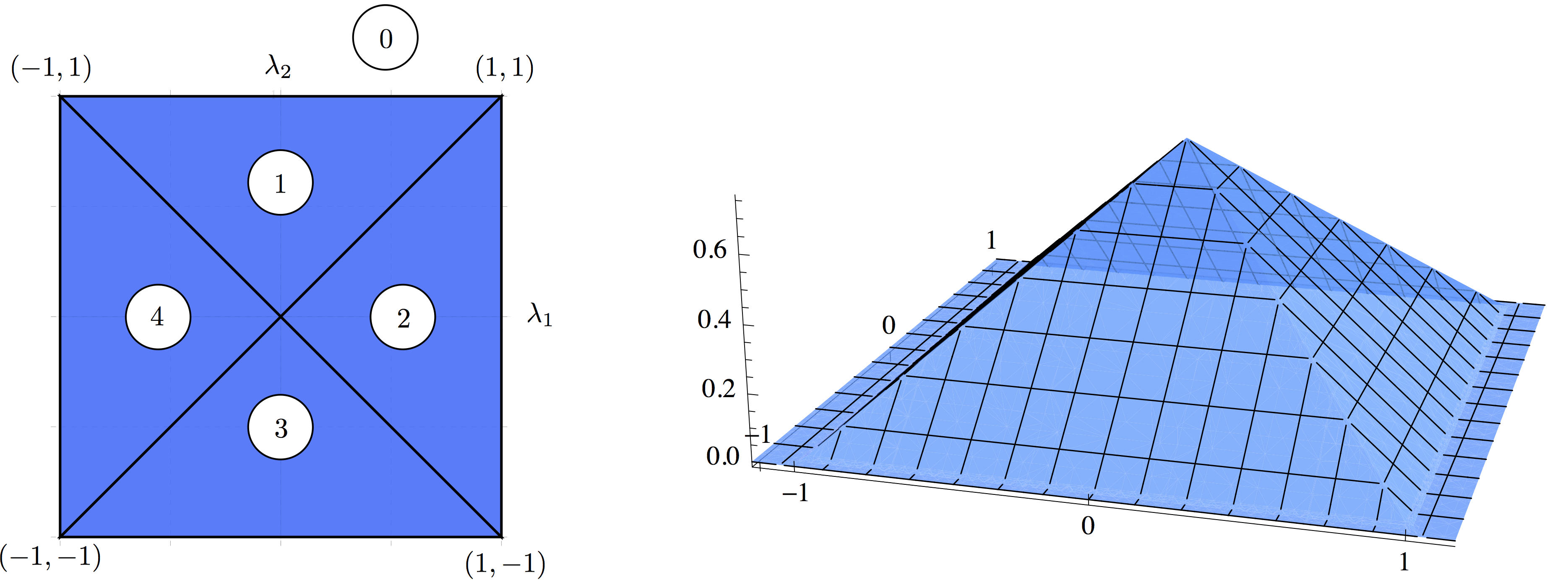
Figure 5.2: Two Qubits. (a) Abelian moment polytope for two qubits and its decomposition into four bounded regular chambers separated by the critical walls (thick lines). (b) Density function of the Abelian Duistermaat–Heckman measure.

We now compute the non-Abelian Duistermaat–Heckman measure by using the derivative principle. Observe that $\partial_{\alpha_{1}}\partial_{\alpha_{2}}f_{T}\equiv 0$ away from the critical walls. On the walls we have to be more careful, since the density function is not twice differentiable there. The horizontal and vertical walls do not carry any measure, since they are constant in one of the two coordinate directions. However, this is not so on the diagonal; and we readily find by integrating against a test function that $\partial_{\alpha_{1}}\partial_{\alpha_{2}}\mathbf{P}_{T}|_{\mathbbm{R}^{2}_{>0}}$ is equal to Lebesgue measure on the non-Abelian moment polytope $\Delta_{K}=\{\vec{\lambda}\in[0,1]^{2}:\lambda_{1}=\lambda_{2}\}$. According to the derivative principle (5.19) we obtain the non-Abelian Duistermaat–Heckman measure $\mathbf{P}_{K}$ by multiplying this result with $p_{K}(\vec{\lambda})=\lambda_{1}\lambda_{2}$. Thus,

$$\int d\mathbf{P}_{K}\,f=3\int_{0}^{1}d\lambda_{1}\,\lambda_{1}^{2}\,f(\lambda_{1},\lambda_{1})$$

for all test functions $f$ on $\mathbbm{R}^{2}_{\geq 0}$. By a simple transformation of variables, we conclude that the joint distribution of the maximal local eigenvalues of a random pure state of two qubits is given by

$$\int d\mathbf{P}_{\operatorname{spec}}\,g=24\int_{0.5}^{1}d\lambda_{1,1}\,(\lambda_{1,1}-0.5)^{2}\,g(\lambda_{1,1},\lambda_{1,1})$$

for all test functions $g=g(\lambda_{1,1},\lambda_{2,1})$. This eigenvalue distribution has been computed more generally for bipartite pure states chosen at random from $\mathbbm{C}^{a}\otimes\mathbbm{C}^{b}$ [LP88, ZS01]. We will further below show how it can be obtained as a direct consequence of the derivative principle.

We now consider the case of three qubits ($n=3$). The eight weights of $\mathbbm{C}^{2}\otimes\mathbbm{C}^{2}\otimes\mathbbm{C}^{2}$ are $(\pm 1,\pm 1,\pm 1)$, the vertices of a cube. We will use some shortcuts to reduce the amount of computation required. In Figure 5.3 we have visualized the non-Abelian moment polytope $\Delta_{K}$, which itself is a union of regular chambers. It is of maximal dimension and therefore the non-Abelian Duistermaat–Heckman measure $\mathbf{P}_{K}$ will be absolutely continuous with a piecewise polynomial density function. Since this density necessarily vanishes outside of $\Delta_{K}$, we may start our computation right away by considering the jump over a facet of the non-Abelian moment polytope. Let us thus consider the critical wall spanned by the weights $(1,1,1)$, $(-1,-1,1)$ and $(1,-1,-1)$ (the boundary of the blue chambers in Figure 5.3). It given by the equation $\vec{\lambda}\cdot(-1,1,-1)=-1$ and contains only a minimal number of weights. Thus we may directly apply the non-Abelian jump formula (5.22) with $\xi=(-1,1,-1)/3$. We obtain that the polynomial density function of $\mathbf{P}_{K}$ on the blue chambers in Figure 5.3 is given by

$$\frac{\lambda_{1}\lambda_{2}\lambda_{3}}{4}\frac{(8-1)!}{(8-3-3-1)!}\left(2^{2}(-2)\right)\frac{(-\lambda_{1}+\lambda_{2}-\lambda_{3}+1)^{8-3-3-1}}{(-2)2^{3}4}$$

$$= \frac{7!}{32}\lambda_{1}\lambda_{2}\lambda_{3}\left(1-\lambda_{1}-\lambda_{2}-\lambda_{3}+2\lambda_{2}\right)$$

We now cross the critical wall $\vec{\lambda}\cdot(-1,-1,-1)=-1$ that separates the blue and the green chambers in Figure 5.3. It is spanned by the weights $(1,1,-1)$, $(1,-1,1)$ and $(-1,1,1)$ and is therefore again minimal. By (5.22) with $\xi=(-1,-1,-1)/3$, the density function of $\mathbf{P}_{K}$ changes by the polynomial

$$\frac{\lambda_{1}\lambda_{2}\lambda_{3}}{4}\frac{(8-1)!}{(8-3-3-1)!}2^{3}\frac{(-\lambda_{1}-\lambda_{2}-\lambda_{3}+1)^{8-3-3-1}}{(-2)2^{3}4}$$

$$= -\frac{7!}{32}\lambda_{1}\lambda_{2}\lambda_{3}(1-\lambda_{1}-\lambda_{2}-\lambda_{3})$$

as we cross the wall. It follows that the density function of $\mathbf{P}_{K}$ is on the two green chambers that face the viewer in Figure 5.3 equal to $\frac{7!}{16}\lambda_{1}\lambda_{2}\lambda_{3}\lambda_{2}$. Note that the blue and green chambers together form the part of the three-qubit polytope where $\lambda_{2}=\min_{k}\lambda_{k}$. By using permutation-symmetry to extend the formulas to all of $\Delta_{K}$, we conclude that the non-Abelian Duistermaat–Heckman measure is given by the following piecewise polynomial density function:

$$f_{K}(\lambda_{1},\lambda_{2},\lambda_{3})=\frac{7!}{32}\lambda_{1}\lambda_{2}\lambda_{3}\begin{cases}2\min_{k}\lambda_{k}&\text{in the lower pyramid}\\ 1-\sum_{k=1}^{3}\lambda_{k}+2\min_{k}\lambda_{k}&\text{in the upper pyramid}\\ 0&\text{otherwise}\end{cases}$$

As in the case of two qubits, it is straightforward to deduce from this the marginal eigenvalue distribution of a random pure state of three qubits.

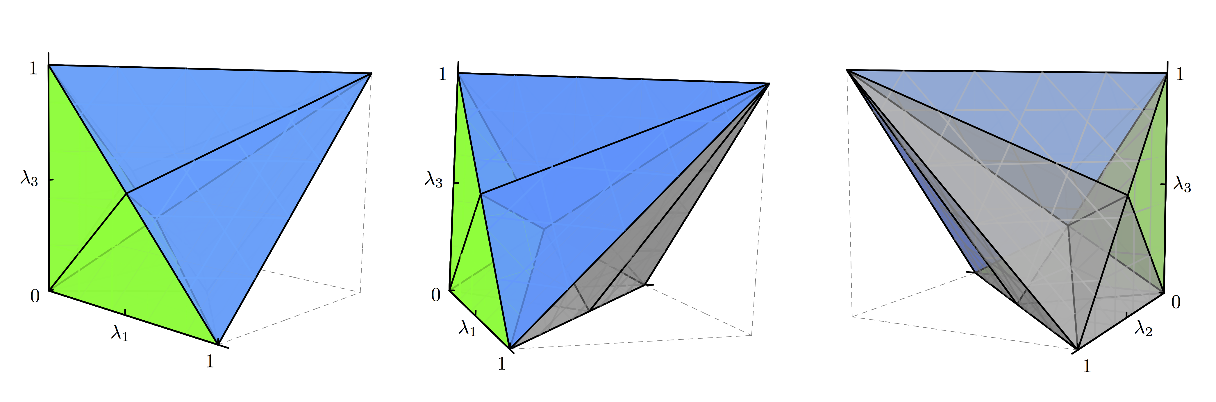
Figure 5.3: Three Qubits. Non-Abelian moment polytope and its decomposition into twelve regular chambers (from three different perspectives).

Bosons

We now turn to random pure states of $n$ bosonic qubits, with Hilbert space $\mathcal{H}=\operatorname{Sym}^{n}(\mathbbm{C}^{2})$. Let $K=\operatorname{SU}(2)$. We identify $i\mathfrak{t}^{*}\cong\mathbbm{R}$ in the same way as above. Thus the positive root is $2$, the occupation number basis vectors in $\operatorname{Sym}^{n}(\mathbbm{C}^{2})$ are weight vectors of weight $-n,-n+2,\dots,n\in\mathbbm{Z}$, and the Abelian moment polytope is $\Delta_{T}=[-n,n]$.

We apply Section 5.3 starting from the left-hand side unbounded chamber $\{\lambda_{1}\leq-n\}$ and successively cross the critical walls, which are points and correspond to a single weight each. At each point $m=-n,-n+2,\dots,n$, the jump formula (5.14) shows that the Abelian measure changes by

$$\frac{1}{1}\frac{((n+1)-1)!}{((n+1)-1-1)!}\frac{(\lambda_{1}-m)^{(n+1)-1-1}}{\prod_{m\neq m^{\prime}=-n,-n+2,\dots,n}(m^{\prime}-m)}$$

$$=\; n\frac{(\lambda_{1}-m)^{n-1}}{\prod_{m\neq m^{\prime}=-n,-n+2,\dots,n}(m^{\prime}-m)}$$

$$=\; \frac{1}{2^{n}(n-1)!}(-1)^{(n+m)/2}\binom{n}{\frac{n+m}{2}}(\lambda_{1}-m)^{n-1}.$$

It follows that the Abelian Duistermaat–Heckman density has Lebesgue density

$$f_{T}(\lambda_{1})=\frac{1}{2^{n}(n-1)!}\sum_{m=-n,-n+2,\dots,n}(-1)^{(n+m)/2}\binom{n}{\frac{n+m}{2}}(\lambda_{1}-m)^{n-1}_{+},$$ (5.23)

where we set $(\lambda_{1}-m)^{n-1}_{+}:=(\lambda_{1}-m)^{n-1}$ for $\lambda_{1}\geq m$ and $0$ otherwise. Amusingly, (5.23) is precisely the probability density of a sum of $n$ independent random variables that are each distributed uniformly in the interval $[-1,1]$ [Fel71, §I.9, Theorem 1a]. It follows from the derivative principle that the non-Abelian measure has Lebesgue density

$$f_{K}(\lambda_{1})=\frac{-\lambda_{1}}{2^{n-1}(n-2)!}\sum_{m=-n,-n+2,\dots,n}(-1)^{(n+m)/2}\binom{n}{\frac{n+m}{2}}(\lambda_{1}-m)^{n-2}_{+},$$

on $[0,\infty)$, which can be readily translated into, e.g., the distribution of the maximal local eigenvalue. See Figure 5.4 for an illustration.

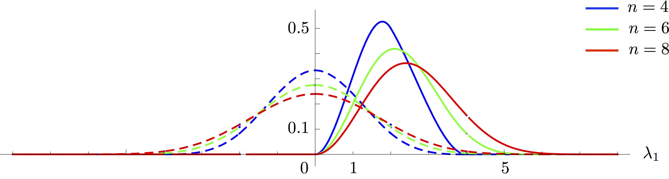
Figure 5.4: Bosonic qubits. Densities of the Abelian (dashed) and of the non-Abelian (solid) Duistermaat–Heckman measure of $\operatorname{Sym}^{n}(\mathbbm{C}^{2})$ for various particle numbers $n$.

As an application, we compute the average value of the linear entropy of entanglement (4.11) for a random pure state of $n$ bosonic qubits. For a bosonic state $\rho$ on $\mathcal{H}$, it is given by

$$E(\rho)=1-\operatorname{tr}\rho_{1}^{2},$$

where $\rho_{1}$ denotes the one-body reduced density matrix.

Lemma .

The average linear entropy of entanglement of a random pure state of $n$ bosonic qubits is equal to $1/2-1/(2n)$.

Proof.

The average linear entropy of entanglement is given by

$$\int d\rho\,E(\rho)=\int d\mathbf{P}_{\operatorname{spec}}(\vec{\lambda}_{1})\left(1-(\lambda_{1,1}^{2}+\lambda_{1,2}^{2})\right)=\frac{1}{2}-\frac{1}{2n^{2}}\int d\mathbf{P}_{K}(\lambda_{1})\lambda_{1}^{2}.$$

To evaluate the right-hand side, we observe that $\lambda_{1}^{2}$ vanishes at $\lambda_{1}=0$, the boundary of the Weyl chamber; thus we may use (5.20) and take limits to reduce to an integral over the Abelian measure. We obtain

$$\int d\mathbf{P}_{K}(\lambda_{1})\lambda_{1}^{2}=\int_{0}^{\infty}d\mathbf{P}_{T}(\lambda_{1})\partial_{2\lambda_{1}}(\lambda_{1}\lambda_{1}^{2})=3\int_{-\infty}^{\infty}d\mathbf{P}_{T}(\lambda_{1})\lambda_{1}^{2},$$ (5.24)

where we have used that $\mathbf{P}_{T}$ is symmetric about the origin. The right-hand side integral is the variance of $\mathbf{P}_{T}$. But recall that $\mathbf{P}_{T}$ is the distribution of a sum of independent random variables that are uniformly distributed on $[-1,1]$. Since the variance of each summand is $1/3$ and it is additive for independent sums, we find that (5.24) is precisely equal to $n$. By plugging this into the first formula, we conclude that, indeed, $\int d\rho\,E(\rho)=1/2-1/(2n)$. ∎

In accordance with the concentration of measure phenomenon, $\rho_{1}\rightarrow\mathbbm{1}/2$ in distribution as $n\rightarrow\infty$. We remark that our result agrees with [MDV12, Theorem 34] if one works out the quantities left uncalculated therein. Note that the proof illustrates the power of the derivative principle: Instead of explicitly computing the average over the eigenvalue distribution, we reduced to an average over the Abelian measure, whose structure we could then exploit.

Bipartite Systems

We conclude this series of examples by giving a concise derivation of the marginal eigenvalue distribution of a random bipartite pure state $\rho$ on $\mathcal{H}=\mathbbm{C}^{a}\otimes\mathbbm{C}^{b}$. Without loss of generality, assume that $a\leq b$. By Chapter 2, it suffices to derive the distribution of eigenvalues of $\rho_{A}$. It will be convenient to work with $K=\operatorname{U}(a)$ rather than the special unitary group, so that we may identify $i\mathfrak{t}^{*}\cong\mathbbm{R}^{a}$.

We first compute the Abelian Duistermaat–Heckman measure $\mathbf{P}_{T}$. For this, observe that the product basis vectors $\ket{ij}\in\mathbbm{C}^{a}\otimes\mathbbm{C}^{b}$ are weight vectors with weight the $i$-th standard basis vector of $\mathbbm{R}^{a}$. Thus $\Delta_{T}$ is equal to the convex hull of these unit vectors, i.e., to the standard simplex $\Delta_{a}$. By (5.10), the density function of $\mathbf{P}_{T}$ with respect to Lebesgue measure on $\Delta_{T}$ can thus be computed in the following way:

$$f_{T}(\vec{\lambda}_{A})=\; \operatorname{vol}\leavevmode\nobreak\ \{(p_{i,j})\in\mathbbm{R}^{ab}_{\geq 0}:\sum_{j=1}^{b}p_{i,j}=\lambda_{A,i}\,(\forall i=1,\dots,a)\}$$

$$=\; \prod_{i=1}^{a}\operatorname{vol}\leavevmode\nobreak\ \{(p_{j})\in\mathbbm{R}^{b}_{\geq 0}:\sum_{j=1}^{b}p_{j}=\lambda_{A,i}\}$$

$$\propto\; \prod_{i=1}^{a}\lambda_{A,i}^{b-1},$$

since each factor is the volume of a $(b-1)$-dimensional simplex. We now consider the negative partial derivative in the direction in the positive roots: Since there are $\binom{a}{2}$ positive roots,

$$\left(\prod_{i<j}\partial_{\lambda_{A,j}-\lambda_{A,i}}\right)\left(\prod_{i=1}^{a}\lambda_{A,i}^{b-1}\right)$$

is a polynomial of degree no more than $a(b-1)-\binom{a}{2}$. Since we differentiate each variable at most $a-1$ times, the result will be a multiple of the symmetric polynomial $\prod_{i=1}^{a}\lambda_{A,i}^{b-a}$. On the other hand, the result is evidently antisymmetric in the variables and so will be a multiple of the Vandermonde determinant $p_{A}(\vec{\lambda}_{A})$. Since the degrees add up, $a(b-a)+\binom{a}{2}=a(b-1)-\binom{a}{2}$ it follows at once that

$$\left(\prod_{i<j}\partial_{\lambda_{A,j}-\lambda_{A,i}}\right)\left(\prod_{i=1}^{a}\lambda_{A,i}^{b-1}\right)\propto\left(\prod_{i=1}^{a}\lambda_{A,i}^{b-a}\right)p_{a}(\vec{\lambda}_{A})$$

Thus we conclude from the derivative principle (5.19) that the eigenvalue distribution of $\rho_{A}$ is proportional to

$$f_{K}(\vec{\lambda}_{A})\propto\left(\prod_{i=1}^{a}\lambda_{A,i}^{b-a}\right)p^{2}_{a}(\vec{\lambda}_{A})$$ (5.25)

on $\Delta_{a,+}=\{\vec{\lambda}_{A}\in\Delta_{a}:\lambda_{A,1}\geq\dots\geq\lambda_{A,a}\}$, the intersection of $\Delta_{a}$ with the positive Weyl chamber, which is the non-Abelian moment polytope for the action of $K=\operatorname{U}(a)$. This is the well-known formula from [LP88, ZS01]. In mathematics, the distribution of $\rho_{A}$ is also known as a normalized Wishart ensemble (see, e.g., [ASY14]). Since $\rho_{A}$ and $\rho_{B}$ have the same non-zero eigenvalues (Chapter 2), it follows immediately from (5.25) that the joint distribution of the marginal eigenvalues of both $\rho_{A}$ and $\rho_{B}$ is given by

$$\int d\mathbf{P}_{\operatorname{spec}}\,f\propto\int_{\Delta_{a,+}}d\vec{\lambda}_{A}\left(\prod_{i=1}^{a}\lambda_{A,i}^{b-a}\right)p_{a}^{2}(\vec{\lambda}_{A})\,f(\vec{\lambda}_{A},\vec{\lambda}_{A})$$ (5.26)

for all test functions $f=f(\vec{\lambda}_{A},\vec{\lambda}_{B})$. For $a=b=d$, this is precisely (5.4) in Section 5.2.

5.6 Discussion

Random ensembles of states have long been studied in quantum statistical physics. In fact, Lloyd and Pagels had derived (5.25) out of thermodynamic considerations [LP88]. More recently, the typical behavior of canonical states, i.e., states that are obtained by computing the reduced density matrix of the uniform state on a subspace (encoding the energy constraint) of the system–bath Hilbert space, have been considered [PSW06, Llo06, GLTZ06], and the average von Neumann entropy of a subsystem [Lub78, Pag93] has featured in the analysis of the black hole entropy paradox [HP07]. Apart from their import from the perspective of the quantum marginal problem, random states of multipartite systems are also relevant in quantum information theory. For example, conditional entropies and mutual informations are central quantities in entanglement theory. Since they are functions of the eigenvalues only they can be studied in the framework of this chapter (e.g., in the case of tripartite pure states). Remarkable recent progress has been made by analyzing the entanglement properties of the two-body reduced density matrix $\rho_{AB}$ of a randomly-chosen tripartite pure state [HLSW04, HLW06, ASY14, ASY12, CNY12]. In all these applications, most known results are for high-dimensional Hilbert spaces, where the powerful concentration of measure phenomenon occurs. In contrast, our exact algorithms require no such assumption and are instead well-suited for low-dimensional systems, which previously remained inaccessible. It would be highly desirable to find a common meeting ground for both techniques that would allow for an interpolation between the combinatorial and the analytical regime (cf. [BG12, BP14]).

Chapter 6 Interlude: Computing Multiplicities of Lie Group Representations

In this chapter we consider the classical branching or subgroup restriction problem in representation theory, which asks for the multiplicity of an irreducible representation of a subgroup $K\subseteq K^{\prime}$ in the restriction of an irreducible representation of $K^{\prime}$. In the case of compact, connected Lie groups, we provide a polynomial-time algorithm for this problem—based on a finite-difference formula for the multiplicities and Barvinok’s algorithm for counting integral points in polytopes. Our algorithm is also applicable to the Kronecker coefficients of the symmetric group, which play an important role in the geometric complexity theory approach to the $\mathbf{P}$ vs. $\mathbf{NP}$ problem. Whereas the computation of Kronecker coefficients is known to be $\#\mathbf{P}$-hard for Young diagrams with an arbitrary number of rows, our algorithm computes them in polynomial time if the number of rows is bounded. The finite-difference formula that we use is a discrete analogue of the derivative principle that was used in the preceding chapter. This connection can be made precise, as the asymptotic growth rates of multiplicities are directly related to the measures that we had computed in the preceding chapter. We complement our results by showing that in geometric complexity theory, such asymptotic information might not directly lead to complexity-theoretic obstructions beyond what can be obtained from moment polytopes. Non-asymptotic information on the multiplicities, such as provided by our algorithm, may therefore be essential in order to find new obstructions in geometric complexity theory.

The results in this chapter have been obtained in collaborations with Matthias Christandl and Brent Doran, and they have appeared in [CDW12]; the first part of Section 6.6 is adapted from the collaboration [CDKW14].

6.1 Summary of Results

The decomposition of Lie group representations into irreducible sub-representations is a fundamental problem in mathematics with a variety of applications to the sciences. In atomic and molecular physics as well as in high-energy physics, this problem has been studied extensively in the context of symmetries [Wey50, WG59, Wig73], perhaps most famously in Ne’eman and Gell-Mann’s “eight-fold way” of elementary particles [Nee61, GM61, GM62]. In pure mathematics, the combinatorial resolution by Knutson and Tao of the problem of decomposing tensor products of irreducible representations of the unitary group has been a recent highlight with a long history of research [Ful00, KT99]. More recently, the representation theory of Lie groups has found novel applications in quantum information [KW01, CM06, Kly06, CSW10] and quantum computation [BCH07, BCH06, Jor08], as well as in the geometric complexity theory approach to the $\mathbf{P}$ vs. $\mathbf{NP}$ problem in computer science [MS01, MS08, BLMW11]. In this chapter, we study the problem of computing multiplicities of Lie group representations:

Problem (Subgroup Restriction Problem, Branching Problem).

Let $\Phi\colon K\rightarrow K^{\prime}$ be a fixed homomorphism of compact, connected Lie groups. What is the multiplicity $m^{\lambda}_{\mu}$ of an irreducible $K$-representation $V_{K,\mu}$ in an irreducible $K$-representation $V_{K^{\prime},\lambda}$, when given as input the highest weights $\mu$ and $\lambda$?

The term subgroup restriction problem comes from the archetypical case where the map $\Phi$ is the inclusion of a subgroup $K\subseteq K^{\prime}$.

The main result of this chapter is a polynomial-time algorithm for the subgroup restriction problem (Section 6.4). It takes as input bitstrings containing the coordinates of the highest weights with respect to fixed bases of fundamental weights. As a direct consequence, for any fixed $\lambda$ and $\mu$ the stretching function $k\mapsto m^{k\lambda}_{k\mu}$ can be evaluated in polynomial time. Another immediate corollary is that the positivity of the coefficients $m^{\lambda}_{\mu}$ can be decided in polynomial time for any fixed homomorphism $\Phi\colon K\rightarrow K^{\prime}$. Mulmuley has conjectured that deciding positivity of the multiplicities $m^{\lambda}_{\mu}$ should be possible in polynomial time even if the group homomorphism $\Phi$ is also part of the input [Mul07]. This is known only for specific families of homomorphisms, such as those corresponding to the Littlewood–Richardson coefficients [KT99, MNS12], and our result can be regarded as supporting evidence for the conjecture. However, any approach to deciding positivity that proceeds by computing the actual multiplicities is of course expected to fail, since the latter problem is well-known to be $\#\mathbf{P}$-hard [Nar06, BI08]. Since representations of compact, connected Lie groups are in one-to-one correspondence with the rational representations of complex, reductive, connected algebraic groups (Section 2.1), our results can also be interpreted in the latter context.

Our polynomial-time algorithm is based on a formula for the multiplicities $m^{\lambda}_{\mu}$ (Section 6.4), which is obtained in three steps: First, we restrict from the group $K^{\prime}$ to its maximal torus $T^{\prime}$. The corresponding weight multiplicities can be computed efficiently by using the classical multiplicity formula of Kostant [Kos59, Coc05] or, in fact, by evaluating a single vector partition function [BGR04, Bli08, Bli10] (Section 6.2). Second, we restrict all weights to a maximal torus $T$ of $K$. Third, we recover the multiplicity of an irreducible $K$-representation by using a finite-difference formula based on Weyl’s character formula: For any $K$-representation $V$, the highest weight multiplicity function $m_{K,V}$ of irreducible $K$-representations and the weight multiplicity function $m_{T,V}$ are related by

$$m_{K,V}=\left.\left[\left(\prod_{\alpha\in R_{K,+}}-D_{\alpha}\right)m_{T,V}\right]\right|_{\Lambda^{*}_{K,+}},$$ (6.1)

where $(D_{\alpha}m)(\lambda)=m(\lambda+\alpha)-m(\lambda)$ denotes the finite-difference operator in direction $\alpha$ (Section 6.3). By carefully combining the first two steps, we obtain a formula for the multiplicities that reduces Section 6.1 to the problem of counting integral points in rational convex polytopes of bounded dimension (Section 6.4). The latter can be done efficiently by using Barvinok’s algorithm [Bar94] (see also [Dye91, CHKM92, DK97, BP99, BBCV06]) and we thus obtain Section 6.4. The multiplicity formula itself has intrinsic interest beyond its application to algorithmics. One immediate insight is a piecewise quasi-polynomiality of the multiplicities and of the stretching function [Mul07].

In Section 6.5, we turn to the computation of the Kronecker coefficients $g_{\alpha,\beta,\gamma}$, which are commonly defined as the multiplicities in the decomposition of tensor products of irreducible representations of the symmetric group $S_{k}$. Kronecker coefficients are notoriously difficult to study, and finding an appropriate combinatorial interpretation is one of the outstanding problems of classical representation theory. Apart from the role for the quantum marginal problem, they appear naturally in geometric complexity theory, where their computation serves as a model problem which has been subject to a number of conjectures [Mul07]. In Section 2.4, we have seen that the Kronecker coefficients can be equivalently defined in terms of the special linear or unitary groups. For Young diagrams of bounded height, this amounts to an instance of Section 6.1 for a fixed group homomorphism $\Phi$. Therefore the Kronecker coefficients can in this case be computed in polynomial time by using Section 6.4. We also get a clean closed-form expression for the Kronecker coefficients (Section 6.5), which not only nicely illustrates the algorithm’s effectiveness, but also implies directly that the problem of computing Kronecker coefficients with unbounded height is in $\mathbf{GapP}$, as first proved in [BI08].

In practice, our algorithm appears to work rather well as long as the rank of the Lie group $G$ is not too large. In the case of Kronecker coefficients for Young diagrams with two rows, we can easily go up to $k=10^{8}$ boxes using commodity hardware. In contrast, all other software packages known to the authors cannot go beyond only a moderate number of boxes ($k=10^{2}$ on the same hardware as used above). Moreover, by distributing the computation of weight multiplicities onto several processors, we have been able to compute Kronecker coefficients for Young diagrams with three rows and $k=10^{5}$ boxes in a couple of minutes. A preliminary implementation of the algorithm is available at [Wal12b]. We hope that our algorithm will provide a useful tool in experimental mathematics, theoretical physics, and geometric complexity theory.

We now turn towards studying the asymptotics of multiplicities. Recall from the fundamental Theorem 2.1 that the moment polytope of a projective subvariety $\mathbbm{X}\subseteq\mathbbm{P}(\mathcal{H})$ can be described as

$$\Delta_{K}(\mathbbm{X})=\overline{\{\lambda/k:m_{K,R^{*}_{k}(\mathbbm{X})}(\lambda)>0\}},$$ (6.2)

where $m_{K,R^{*}_{k}(\mathbbm{X})}(\lambda)$ denotes the multiplicity of the irreducible $K$-representation $V_{G,\lambda}$ in $R^{*}_{k}(\mathbbm{X})$, the dual of the space of regular functions of degree $k$. This suggests to consider the following measure defined as the weak limit of the atomic measures that encode the multiplicities in a fixed degree $k$,

$$\nu_{K,\mathbbm{X}}:=\operatorname*{w-lim}_{k\rightarrow\infty}\frac{1}{k^{d_{K,\mathbbm{X}}}}\sum_{\lambda\in\Lambda^{*}_{K,+}}m_{K,R^{*}_{k}(\mathbbm{X})}(\lambda)\,\delta_{\lambda/k},$$ (6.3)

where $d_{K,\mathbbm{X}}\in\mathbbm{Z}_{\geq 0}$ is the appropriate exponent such that $\nu_{K,\mathbbm{X}}$ has finite, non-zero measure [Oko96]. It has a piecewise-polynomial density function $f_{K,\mathbbm{X}}$ with respect to Lebesgue measure on the moment polytope and its support is the entire moment polytope (both assertions follow from the main result of [Oko96], but probably go back to earlier work). By definition, the measure $\nu_{K,\mathbbm{X}}$ encodes the asymptotic growth rate of multiplicities in the ring of regular functions of the projective variety $\mathbbm{X}$. If $\mathbbm{X}$ is smooth then $\nu_{K,\mathbbm{X}}$ can be given a remarkable geometric interpretation: It is directly related to the Duistermaat–Heckman measure $\mathbf{P}_{K,\mathbbm{X}}$ that we had considered in Chapter 5. This fact holds more generally for smooth projective subvarieties and other symplectic manifolds that can be “quantized” in a certain technical sense [Hec82, GS82b, Sja95, Mei96, Ver98, MS99].

In Section 6.6, we first give a succinct proof of the relation between $\nu_{K,\mathbbm{X}}$ and $\mathbf{P}_{K,\mathbbm{X}}$ in the case where $\mathbbm{X}$ is the full projective space $\mathbbm{P}(\mathcal{H})$. Our argument is based on the observation that the finite difference formula (6.1) “converges” to the derivative principle (5.19) in the limit as $k\rightarrow\infty$, as was also pointed out to us by Allen Knutson. Applied to the quantum marginal problem, we find that the distribution of the one-body reduced density matrices of a random quantum state, as computed in Chapter 5, is directly related to the asymptotic growth of the Kronecker coefficients.

We then consider the applicability of the measures $\nu_{K,\mathbbm{X}}$ to geometric complexity theory. In a nutshell, the main challenge in geometric complexity theory is to show that for certain pairs of projective subvarieties $\mathbbm{X}$ and $\mathbbm{Y}$ one is not contained in the other; this would then imply complexity-theoretic lower bounds. Both the permanent vs. determinant problem, which is equivalent to the $\mathbf{VP}$ vs. $\mathbf{VNP}$ problem [Val79] (an algebraic version of the $\mathbf{P}\neq\mathbf{NP}$ conjecture), as well as the complexity of matrix multiplication [Str69] can be formulated in this framework [MS01, MS08, BI11, BLMW11]. The starting point is the basic observation that

$$\mathbbm{X}\subseteq\mathbbm{Y}\;\Longrightarrow\;m_{K,R^{*}_{k}(\mathbbm{X})}(\lambda)\leq m_{K,R^{*}_{k}(\mathbbm{Y})}(\lambda)$$ (6.4)

for all $\lambda$ and $k\geq 0$. Therefore, the existence of $\lambda$ and $k$ such that $m_{K,R^{*}_{k}(\mathbbm{X})}(\lambda)>m_{K,R^{*}_{k}(\mathbbm{Y})}(\lambda)$ proves that $\mathbbm{X}\not\subseteq\mathbbm{Y}$; such a pair $(\lambda,k)$ is called an obstruction [MS08]. Since computing multiplicities in general coordinate rings is a difficult problem, it is natural to instead study their asymptotic behavior. Following an idea of Strassen [Str06], it has been proposed in [BI11] to consider instead the moment polytopes (6.2), whose geometric interpretation facilitates their computation, as we have seen in Chapter 3. Clearly,

$$\mathbbm{X}\subseteq\mathbbm{Y}\;\Longrightarrow\;\Delta_{K}(\mathbbm{X})\subseteq\Delta_{K}(\mathbbm{Y}).$$ (6.5)

However, preliminary results suggest that the right-hand side moment polytope $\Delta_{K}(\mathbbm{Y})$ might be trivially large for the varieties of interest in geometric complexity theory [BCI11, BI11, Kum11, BLMW11], which would imply that (6.5) is insufficient for finding complexity-theoretic obstructions. It has therefore been suggested recently to study the asymptotic growth of multiplicities as captured by the measures $\nu_{K,\mathbbm{X}}$ (e.g., [GR12, §2.2]). In this context, our contribution is a “no go” result: We show that, in the situations of interest in geometric complexity theory, $\mathbbm{X}\subseteq\mathbbm{Y}$ implies that $d_{K,\mathbbm{X}}<d_{K,\mathbbm{Y}}$ for the exponents in the definition (6.3) of the measures (Section 6.6). Therefore, we cannot deduce from (6.3) and (6.4) a criterion of the form

“$$\mathbbm{X}\subseteq\mathbbm{Y}\;\Longrightarrow\;f_{K,\mathbbm{X}}(\lambda)\leq f_{K,\mathbbm{Y}}(\lambda)$$”,

since we need to divide by different powers of $k$ in the definition of the weak limit. In this sense, the measures $\nu_{K,\mathbbm{X}}$ do not directly give rise to new obstructions, indicating that a more refined understanding of the behavior of multiplicities in coordinate rings might be required.

6.2 Weight Multiplicities

Throughout this chapter, we will use the notations and conventions of Section 2.1; however, we will label all objects such as weight lattices, irreducible representations, etc. by the compact connected Lie group $K$, since we will mostly not need its complexification $G$ explicitly. Recall that the irreducible representations of $K$ are labeled by their highest weight in $\Lambda^{*}_{K,+}$. An arbitrary finite-dimensional representation $V$ can always be decomposed into irreducible sub-representations,

$$V\cong\bigoplus_{\lambda\in\Lambda^{*}_{K,+}}m_{K,V}(\lambda)\,V_{K,\lambda}.$$

We will call the function $m_{K,V}$ thus defined the highest weight multiplicity function.

We may similar decompose $V$ into irreducible representations of the maximal torus $T\subseteq K$, which we recall are one-dimensional and labeled by elements of the weight lattice $\Lambda^{*}_{K}$. We thus obtain the decomposition into weight spaces

$$V=\bigoplus_{\omega\in\Lambda^{*}_{K}}V_{\omega}.$$

We will call $m_{T,V}(\omega)=\dim V_{\omega}$ the weight multiplicity function. An equivalent way of encoding the weight multiplicities is in terms of the (formal) character,

$$\operatorname{ch}V=\sum_{\omega}m_{T,V}(\omega)\,e^{\omega},$$

Formally, $\operatorname{ch}V$ is an element of the group ring $\mathbbm{Z}[\Lambda^{*}_{K}]$, which consists of (finite) linear combinations of basis elements $e^{\omega}$ for each weight $\omega\in\Lambda^{*}_{K}$; the multiplication is defined by $e^{\omega}e^{\omega^{\prime}}=e^{\omega+\omega^{\prime}}$ (see, e.g., [Kna02]). We may identify elements of the group ring with integer-valued functions on the weight lattice $\Lambda^{*}_{K}$ that have finite support. In this way, the character $\operatorname{ch}V$ and the weight multiplicity function $m_{T,V}$ become one and the same object. We remark that $\operatorname{ch}V$ is directly related to the usual definition of a character as the trace of the representation: we have that $\operatorname{tr}\Pi(\exp(X))=\sum_{\omega}m_{T,V}(\omega)e^{(\omega,X)}$ for all $X\in\mathfrak{t}$.

Weyl and Kostant Formulas

The character of an irreducible representation $V_{K,\lambda}$ is given by the famous Weyl character formula

$$\operatorname{ch}V_{K,\lambda}=\frac{\sum_{w\in W_{K}}(-1)^{l(w)}\,e^{w(\lambda+\rho_{K})-\rho_{K}}}{\prod_{\alpha\in R_{K,+}}\left(1-e^{-\alpha}\right)}.$$ (6.6)

where $\rho_{K}=\sum_{\alpha\in R_{K,+}}\alpha/2\in\Lambda^{*}_{K}$ is known as the Weyl vector. To make sense of the right-hand side fraction, we need to work in the larger ring of functions that are supported in a finite number of “cones” of the form

$$\{\omega-\sum_{\alpha}x_{\alpha}\alpha:(x_{\alpha})\in\mathbbm{Z}^{R_{K,+}}_{\geq 0}\}.$$

This restriction ensures that multiplication is still well-defined [Kna02] (unlike for general functions!). We find that the denominator in (6.6) is indeed invertible, with inverse

$$\frac{1}{\prod_{\alpha\in R_{K,+}}\left(1-e^{-\alpha}\right)}=\prod_{\mathclap{\alpha\in R_{K,+}}}\left(1+e^{-\alpha}+e^{-2\alpha}+\dots\right)=\sum_{\mathclap{\omega\in\Lambda^{*}_{K}}}\phi_{R_{K,+}}(\omega)e^{-\omega}.$$

In the last equation we have introduced the Kostant partition function

$$\phi_{R_{K,+}}(\omega)=\#\{(x_{\alpha})\in\mathbbm{Z}^{R_{K,+}}_{\geq 0}:\sum_{\alpha}x_{\alpha}\alpha=\omega\},$$

which counts the number of ways that a weight can be written as a sum of positive roots (this number is always finite since the positive roots span a proper cone). It follows directly from the above that

$$\operatorname{ch}V_{K,\lambda}= \sum_{w\in W_{K}}(-1)^{l(w)}\sum_{\omega\in\Lambda^{*}_{K}}\phi_{R_{K,+}}(\omega)e^{w(\lambda+\rho)-\rho-\omega}$$

$$= \sum_{\omega\in\Lambda^{*}_{K}}\sum_{w\in W_{K}}(-1)^{l(w)}\,\phi_{R_{K,+}}(w(\lambda+\rho)-\rho-\omega)e^{\omega}.$$

Thus the multiplicity of a weight $\omega$ in an irreducible representation $V_{K,\lambda}$ is given by the well-known Kostant multiplicity formula [Kos59],

$$m_{T,V_{K,\lambda}}(\omega)=\sum_{w\in W_{K}}(-1)^{l(w)}\,\phi_{R_{K,+}}(w(\lambda+\rho)-\rho-\omega).$$ (6.7)

For any fixed group $K$, the Kostant partition function can be evaluated in polynomial time by using Barvinok’s algorithm [Bar94], since it amounts to counting integral points in a convex polytope in an ambient space of fixed dimension. Therefore, weight multiplicities for fixed groups $K$ can be computed efficiently. This idea has been implemented by Cochet [Coc05] to compute weight multiplicities for the classical Lie algebras (but using the method of [BBCV06] instead of Barvinok’s algorithm). We note that the problem of computing weight multiplicities is of course a special case of Section 6.1 where $K$ is the maximal torus of $K^{\prime}$.

Weight Multiplicities as a Single Partition Function

If the group $K$ is semisimple, then it is known that we can find $s,t\in\mathbbm{Z}_{\geq 0}$ and $\mathbbm{Z}$-linear maps $A\colon\mathbbm{Z}^{s}\rightarrow\mathbbm{Z}^{t}$, $B\colon\Lambda^{*}_{K}\oplus\Lambda^{*}_{K}\rightarrow\mathbbm{Z}^{t}$ such that

$$m_{T,V_{K,\lambda}}(\omega)=\phi_{A}\left(B\left(\begin{smallmatrix}\lambda\\ \omega\end{smallmatrix}\right)\right)$$ (6.8)

for all $\lambda\in\Lambda^{*}_{K,+},\omega\in\Lambda^{*}_{K}$, where $\phi_{A}$ is a vector partition function defined by

$$\phi_{A}(y)=\#\{x\in\mathbbm{Z}^{s}_{\geq 0}:Ax=y\}.$$ (6.9)

Note that this improves over the Kostant multiplicity formula (6.7), where weight multiplicities are expressed as an alternating sum over several invocations of a vector partition function. In particular, (6.8) is an evidently positive formula. Billey, Guillemin, and Rassart have constructed (6.8) for the Lie group $K=\operatorname{SU}(d)$ [BGR04] by using Gelfand–Tsetlin patterns [GT88]; the general construction is due to Bliem [Bli08] based on Littelmann patterns [Lit98].

We note that the assumption of semisimplicity for (6.8) is not a restriction. If $K$ is a general compact connected Lie group then its Lie algebra can always decomposed as

$$\mathfrak{k}=[\mathfrak{k},\mathfrak{k}]\oplus\mathfrak{z},$$

where $[\mathfrak{k},\mathfrak{k}]$ is the Lie algebra of a compact connected semisimple Lie group $K_{\operatorname{ss}}$ and $\mathfrak{z}$ the Lie algebra of the center $Z(K)$ of $K$. By Schur’s lemma (2.23), each element of the center acts by a scalar on an irreducible representation $V_{K,\lambda}$. Therefore, all weights that appear in $V_{K,\lambda}$ have the same restriction to $\mathfrak{z}$. It follows that

$$m_{T,V_{K,\lambda}}(\omega)=\begin{cases}m_{T_{\operatorname{ss}},V_{K_{\operatorname{ss}},\lambda_{\operatorname{ss}}}}(\omega_{\operatorname{ss}})&\text{if $\omega_{z}=\lambda_{z}$},\\ 0&\text{otherwise},\end{cases}$$ (6.10)

where we write $\omega=\omega_{\operatorname{ss}}\oplus\omega_{z}$ according to the corresponding decomposition of weight lattices $\Lambda^{*}_{K}=\Lambda^{*}_{K_{\operatorname{ss}}}\oplus\Lambda^{*}_{Z(K)}$, and likewise for $\lambda$. These multiplicities can thus be evaluated by using (6.8).

6.3 The Finite Difference Formula

Let $V$ be a finite-dimensional representation of the compact connected Lie group $K$. In the preceding section we have seen that we can compute the weight multiplicity function $m_{T,V}$ from the highest weight multiplicity function $m_{K,V}$ by using one of the classical formulas (6.6) and (6.7), or by evaluating the vector partition function (6.8) of Bliem. By “inverting” the Weyl character formula, the converse can also be achieved:

Lemma .

For any finite-dimensional $K$-representation $V$, we have that

$$m_{K,V}=\left.\left[\left(\prod_{\alpha\in R_{K,+}}-D_{\alpha}\right)m_{T,V}\right]\right|_{\Lambda^{*}_{K,+}},$$ (6.11)

where $(D_{\alpha}m)(\lambda)=m(\lambda+\alpha)-m(\lambda)$ is the finite-difference operator in direction $\alpha$.

Proof.

By linearity, it suffices to establish the lemma for an irreducible representation $V=V_{K,\lambda}$. The Weyl character formula (6.6) can be rewritten in the form

$$\prod_{\alpha>0}\left(1-e^{-\alpha}\right)\operatorname{ch}V_{K,\lambda}=\sum_{w\in W_{K}}\det(w)\,e^{w(\lambda+\rho_{K})-\rho_{K}}.$$ (6.12)

Under our identification of elements in $\mathbbm{Z}[\Lambda^{*}_{K}]$ with functions on the weight lattice, multiplication with $\left(e^{-\alpha}-1\right)$ amounts to applying the finite-difference operator $D_{\alpha}$. Thus the left-hand side of (6.12) can be identified with $\left(\prod_{\alpha\in R_{K,+}}\!-D_{\alpha}\right)m_{T,V_{K,\lambda}}$.

Now consider the right-hand side of (6.12). Since $\lambda+\rho_{K}$ is a strictly dominant weight in $\Lambda^{*}_{K,>0}=\Lambda^{*}_{K}\cap i\mathfrak{t}^{*}_{>0}$, it is sent by any Weyl group element $w\neq 1$ to the interior of a different Weyl chamber. That is, for any $w\neq 1$ there exists a positive root $\alpha\in R_{K,+}$ such that $(w(\lambda+\rho_{K}),H_{\alpha})<0$. Therefore $w(\lambda+\rho_{K})-\rho_{K}$ is a dominant weight if only if $w=1$, in which case it is equal to $\lambda$. It follows that the right-hand side of (6.12) identifies with a function on the weight lattice whose restriction to $\Lambda^{*}_{K,+}$ is equal to the indicator function of $\{\lambda\}$, i.e., to the highest weight multiplicity function $m_{K,V_{K,\lambda}}=\delta_{\lambda}$ of $V_{K,\lambda}$. ∎

The idea of using (6.6) for determining multiplicities of irreducible representations goes back at least to Steinberg [Ste61], who proved a formula for the multiplicity $c^{\alpha,\beta}_{\lambda}$ of an irreducible representation $V_{K,\lambda}$ in the tensor product $V_{K,\alpha}\otimes V_{K,\beta}$. These multiplicities $c^{\alpha,\beta}_{\lambda}$ are called the Littlewood–Richardson coefficients for $K$ (cf. Section 2.4). Steinberg’s formula involves an alternating sum over the Kostant partition function (6.7) and can therefore be evaluated efficiently as described by Cochet [Coc05]. De Loera and McAllister give another method for computing Littlewood–Richardson coefficients [DLM06], which applies Barvinok’s algorithm to a result by Berenstein and Zelevinsky [BZ01]. Since the tensor products of irreducible $K$-representations are just the irreducible representations of $K\times K$, the problem of computing Littlewood–Richardson coefficients is again a special case of Section 6.1. The Clebsch–Gordan series in quantum mechanics is routinely derived in a similar fashion (it corresponds to the case $K=\operatorname{SU}(2)$).

An immediate consequence of Section 6.3 is that there exists a finite set of weights $\Gamma_{K}\subseteq\Lambda^{*}_{K}$ and coefficients $c_{\gamma}\in\mathbbm{Z}$ such that

$$m_{K,V}(\lambda)=\sum_{\gamma\in\Gamma_{K}}c_{\gamma}\,m_{T,V}(\lambda+\gamma).$$ (6.13)

In fact, it is not hard to see that the coefficients can be defined by the expansion $\prod_{\alpha\in R_{K,+}}\!\left(1-e^{-\alpha}\right)=\sum_{\gamma\in\Gamma_{K}}c_{\gamma}e^{-\gamma}$.

6.4 Multiplicities for the Subgroup Restriction Problem

Now let $\Phi\colon K\rightarrow K^{\prime}$ be a homomorphism of compact, connected Lie groups and $\phi\colon\mathfrak{k}\rightarrow\mathfrak{k^{\prime}}$ the induced homomorphism of Lie algebras. We choose maximal tori $T\subseteq K$ and $T^{\prime}\subseteq K^{\prime}$ such that $\Phi(T)\subseteq T^{\prime}$. Then $\phi(\mathfrak{t})\subseteq\mathfrak{t^{\prime}}$, and the (complexified) dual map restricts to a $\mathbbm{Z}$-linear map between the weight lattices, which we shall denote by $\phi^{*}\colon\Lambda^{*}_{K^{\prime}}\rightarrow\Lambda^{*}_{K}$. Indeed, the following lemma follows readily from the definitions:

Lemma .

Let $V$ be a representation of $K^{\prime}$ and $\ket{\psi}\in V$ a weight vector of weight $\omega\in\Lambda^{*}_{K^{\prime}}$. If we restrict the action to $K$ via $\Phi\colon K\rightarrow K^{\prime}$ then $\ket{\psi}$ is a weight vector of weight $\phi^{*}\omega\in\Lambda^{*}_{K}$.

As alluded to in the introduction, our strategy for solving the subgroup restriction problem then is the following: Given an irreducible representation $V_{K^{\prime},\lambda}$ of $K^{\prime}$, we can determine its weight multiplicities with respect to the maximal torus $T_{K^{\prime}}$ by using any of the formulas from Section 6.2. We then obtain the weight multiplicities for $T$ by restricting as in Section 6.4. Finally, we reconstruct the multiplicity of an irreducible representation $V_{K,\mu}$ by using the finite-difference formula from Section 6.3. If this procedure were to be translated directly into an algorithm, the runtime would be polynomial in the coefficients of $\lambda$, i.e., exponential in their bitlength (cf. the branching formula by Straumann [Str65]). Indeed, the number of weights generically grows polynomially and can even be of the order of the dimension of the irreducible representation $V_{K^{\prime},\lambda}$, which according to the Weyl dimension formula is given by

$$\dim V_{K^{\prime},\lambda}=\prod_{\alpha\in R_{K^{\prime},+}}\frac{(\lambda+\rho_{K^{\prime}},H_{\alpha})}{(\rho_{K^{\prime}},H_{\alpha})}.$$ (6.14)

It is however possible to combine (6.8) with the restriction map $\phi^{*}$ in a way that will subsequently give rise to an algorithm that runs in polynomial time in the bitlength of the input:

Proposition .

Let $\Phi\colon K\rightarrow K^{\prime}$ be a homomorphism of compact connected Lie groups. Then we can construct $\mathbbm{Z}$-linear maps $A^{\prime}\colon\mathbbm{Z}^{s+s^{\prime}}\rightarrow\mathbbm{Z}^{u}$ and $B^{\prime}\colon\Lambda^{*}_{K^{\prime}}\oplus\Lambda^{*}_{K}\rightarrow\mathbbm{Z}^{u}$ with $s=O(r_{K^{\prime}}^{2})$, $s^{\prime}=r_{K^{\prime}_{\operatorname{ss}}}\leq r_{K^{\prime}}$ and $u=O(r_{K^{\prime}}^{2})+r_{K}$ that satisfy the following property: For any two highest weights $\lambda\in\Lambda^{*}_{K^{\prime},+}$ and $\mu\in\Lambda^{*}_{K,+}$, the multiplicity $m^{\lambda}_{\mu}$ is given by

$$m^{\lambda}_{\mu}=\sum_{\gamma\in\Gamma_{K}}c_{\gamma}\,\#\{x^{\prime}\in\mathbbm{Z}^{s}_{\geq 0}\oplus\mathbbm{Z}^{s^{\prime}}:A^{\prime}x^{\prime}=B^{\prime}\left(\begin{smallmatrix}\lambda\\ \mu+\gamma\end{smallmatrix}\right)\},$$ (6.15)

where the set $\Gamma_{K}$ and the coefficients $c_{\gamma}\in\mathbbm{Z}$ are defined as in (6.13).

Proof.

We start with the finite-difference formula in the form (6.13),

$$m^{\lambda}_{\mu}=m_{K,V_{K^{\prime},\lambda}}(\mu)=\sum_{\gamma\in\Gamma_{K}}c_{\gamma}\,m_{T,V_{K^{\prime},\lambda}}(\mu+\gamma).$$

According to Section 6.4, weight multiplicities for $K$ can be expressed in terms of weight multiplicities for $K^{\prime}$:

$$m_{T,V_{K^{\prime},\lambda}}(\omega)=\sum_{\mathclap{\begin{subarray}{c}\omega^{\prime}\in\Lambda^{*}_{K^{\prime}}\\ \phi^{*}\omega^{\prime}=\omega\end{subarray}}}\;m_{T^{\prime},V_{K^{\prime},\lambda}}(\omega^{\prime})=\sum_{\mathclap{\begin{subarray}{c}\omega^{\prime}_{\operatorname{ss}}\in\Lambda^{*}_{K^{\prime}_{\operatorname{ss}}}\\ \phi^{*}(\omega^{\prime}_{\operatorname{ss}}\oplus\lambda_{z})=\omega\end{subarray}}}\;m_{T^{\prime}_{\operatorname{ss}},V_{K^{\prime}_{\operatorname{ss}},\lambda_{\operatorname{ss}}}}(\omega^{\prime}_{\operatorname{ss}}),$$

where we have used (6.10) to reduce to the semisimple part $K^{\prime}_{\operatorname{ss}}\subseteq K^{\prime}$. According to [Bli08], we can find $\mathbbm{Z}$-linear maps $A\colon\mathbbm{Z}^{s}\rightarrow\mathbbm{Z}^{t}$, $B\colon\Lambda^{*}_{K^{\prime}_{\operatorname{ss}}}\oplus\Lambda^{*}_{K^{\prime}_{\operatorname{ss}}}\rightarrow\mathbbm{Z}^{t}$ with $s,t=O(r_{K^{\prime}}^{2})$ such that weight multiplicities for $K^{\prime}_{\operatorname{ss}}$ are given as in (6.8). Thus,

$$\sum_{\mathclap{\begin{subarray}{c}\omega^{\prime}_{\operatorname{ss}}\in\Lambda^{*}_{K^{\prime}_{\operatorname{ss}}}\\ \phi^{*}(\omega^{\prime}_{\operatorname{ss}}\oplus\lambda_{z})=\omega\end{subarray}}}\;m_{T^{\prime}_{\operatorname{ss}},V_{K^{\prime}_{\operatorname{ss}},\lambda_{\operatorname{ss}}}}(\omega^{\prime}_{\operatorname{ss}})=\sum_{\mathclap{\begin{subarray}{c}\omega^{\prime}_{\operatorname{ss}}\in\Lambda^{*}_{K^{\prime}_{\operatorname{ss}}}\\ \phi^{*}(\omega^{\prime}_{\operatorname{ss}}\oplus\lambda_{z})=\omega\end{subarray}}}\;\#\{x\in\mathbbm{Z}^{s}_{\geq 0}:Ax=B\left(\begin{smallmatrix}\lambda_{\operatorname{ss}}\\ \omega^{\prime}_{\operatorname{ss}}\end{smallmatrix}\right)\}.$$

Finally, decompose $B=B_{1}\oplus B_{2}$ according to $\Lambda^{*}_{K^{\prime}_{\operatorname{ss}}}\oplus\Lambda^{*}_{K^{\prime}_{\operatorname{ss}}}$ and $\phi^{*}=\phi^{*}_{\operatorname{ss}}\oplus\phi^{*}_{z}$ according to $\Lambda^{*}_{K}=\Lambda^{*}_{K_{\operatorname{ss}}}\oplus\Lambda^{*}_{Z(K)}$. Then we can rewrite the above in the following way:

$$\#\{(x,\omega^{\prime}_{\operatorname{ss}})\in\mathbbm{Z}^{s}_{\geq 0}\oplus\Lambda^{*}_{K^{\prime}_{\operatorname{ss}}}:Ax=B\left(\begin{smallmatrix}\lambda_{\operatorname{ss}}\\ \omega^{\prime}_{\operatorname{ss}}\end{smallmatrix}\right),\phi^{*}(\omega^{\prime}_{\operatorname{ss}}\oplus\lambda_{z})=\omega\}$$ (6.16)

$$= \#\{(x,\omega^{\prime}_{\operatorname{ss}})\in\mathbbm{Z}^{s}_{\geq 0}\oplus\Lambda^{*}_{K^{\prime}_{\operatorname{ss}}}:Ax=B_{1}\lambda_{\operatorname{ss}}+B_{2}\omega^{\prime}_{\operatorname{ss}},\;\phi^{*}_{\operatorname{ss}}\omega^{\prime}_{\operatorname{ss}}+\phi^{*}_{z}\lambda_{z}=\omega\}$$

$$= \#\{(x,\omega^{\prime}_{\operatorname{ss}})\in\mathbbm{Z}^{s}_{\geq 0}\oplus\Lambda^{*}_{K^{\prime}_{\operatorname{ss}}}:\underbrace{\left(\begin{smallmatrix}A&-B_{2}\\ 0&\phi^{*}_{\operatorname{ss}}\end{smallmatrix}\right)}_{=:A^{\prime}}\left(\begin{smallmatrix}x\\ \omega^{\prime}_{\operatorname{ss}}\end{smallmatrix}\right)=\underbrace{\left(\begin{smallmatrix}B_{1}&0&0\\ 0&-\phi^{*}_{z}&\mathbbm{1}\end{smallmatrix}\right)}_{=:B^{\prime}}\left(\begin{smallmatrix}\lambda_{\operatorname{ss}}\\ \lambda_{z}\\ \omega\end{smallmatrix}\right)\}$$

After choosing a basis of the lattice $\Lambda^{*}_{K^{\prime}_{\operatorname{ss}}}\cong\mathbbm{Z}^{r_{K^{\prime}_{\operatorname{ss}}}}$ we arrive at the asserted formula (with $u=t+r_{K}$). ∎

We note that the proof of Section 6.4 is constructive: The maps $A^{\prime}$ and $B^{\prime}$, whose existence is asserted by the proposition, are defined in (6.16) in terms of the maps $A$ and $B$ constructed explicitly in [Bli08, §4] (or [BGR04, Proof of Theorem 2.1] for $\mathfrak{k}=\mathfrak{su}(d)$). In Section 6.5 we give an illustration in the context of the Kronecker coefficients. If one uses the Kostant multiplicity formula (6.7) rather than Bliem’s formula (6.8) in the proof of Section 6.4 then one obtains at a similar formula for the multiplicities $m^{\lambda}_{\mu}$. After completion of this work, we have learned of [Hec82, (3.5)], which is derived precisely in this spirit (and attributed to Kostant).

Consequences

Let us identify

$$\Lambda^{*}_{K}\cong\mathbbm{Z}^{r_{K}}\text{ and }\Lambda^{*}_{K^{\prime}}\cong\mathbbm{Z}^{r_{K^{\prime}}}$$ (6.17)

according to the bases of fundamental weights. Then the $\mathbbm{Z}$-linear maps $A^{\prime}$ and $B^{\prime}$ in Section 6.4 correspond to matrices with integer entries, which we shall denote by the same symbol. In this way, we find that (6.15) in essence reduces the computation of the multiplicities $m^{\lambda}_{\mu}$ to counting the number of integral points in rational convex polytopes of the form

$$\Delta_{A^{\prime},B^{\prime}}(y)=\{x^{\prime}\in\mathbbm{R}^{s}_{\geq 0}\oplus\mathbbm{R}^{s^{\prime}}:A^{\prime}x^{\prime}=B^{\prime}y\}.$$ (6.18)

parametrized by $y\in\mathbbm{Z}^{r_{K^{\prime}}+r_{K}}$. It is well-known that this number

$$n(y)=\#(\Delta_{A^{\prime},B^{\prime}}(y)\cap\mathbbm{Z}^{s+s^{\prime}})$$

is a piecewise quasi-polynomial function of $y$ [CL98]. That is, there exists a decomposition of $\mathbbm{Z}^{r_{K^{\prime}}+r_{K}}$ into polyhedral chambers such that on each chamber $C$ the function $n(y)$ is given by a single quasi-polynomial, i.e., there exists a sublattice $L\subseteq\mathbbm{Z}^{r_{K^{\prime}}+r_{K}}$ of finite index and polynomials $p_{z}$ with rational coefficients, labeled by the finitely many points $z\in\mathbbm{Z}^{r_{K^{\prime}}+r_{K}}/L$, such that $n(y)=p_{[y]}(y)$ for all $y\in\mathbbm{Z}^{r_{K^{\prime}}+r_{K}}$ (cf. [VSB⁺07, §2.2]). It follows that the multiplicities $m^{\lambda}_{\mu}$, too, are piecewise quasi-polynomial functions. While the chambers for $n(y)$ are rational polyhedral cones, it does not follow that the same is true for $m^{\lambda}_{\mu}$ (due to the shifts in (6.15)). However, what remains true is that the stretching function $k\mapsto m^{k\lambda}_{k\mu}$ is a quasi-polynomial function for large $k$. It is more involved to show that this is in fact true for all $k$, as has been observed in [Mul07]; we refer to [MS99] for more general quasi-polynomiality results on polyhedral cones (cf. the discussion in [BV10]).

Polynomial-Time Algorithm for the Subgroup Restriction Problem

We will now formulate our polynomial-time algorithm for the subgroup restriction problem. As we have just explained, (6.15) reduces the computation of the multiplicities $m^{\lambda}_{\mu}$ to counting the number of integral points in rational convex polytopes of the form (6.18). We shall suppose that the highest weights $\lambda$ and $\mu$, which are the input to our algorithm, are given in terms of bitstrings containing coordinates with respect to the identification (6.17). Clearly, for each of the finitely many $\gamma\in\Gamma_{K}$, the polytope $\Delta_{A^{\prime},B^{\prime}}(\lambda,\mu+\gamma)$ defined in (6.18) can be described in polynomial size in the bitlength of the input (e.g., in terms of linear equalities and inequalities), and it can be produced from the input in polynomial time. Therefore we may use Barvinok’s algorithm to compute the number of integral points in each of these polytopes in polynomial time [Bar94]. We thus obtain the following algorithm:

Algorithm .

Let $\Phi\colon K\rightarrow K^{\prime}$ be a homomorphism of compact connected Lie groups. Given as input two highest weights $\lambda\in\Lambda^{*}_{K^{\prime}}\cong\mathbbm{Z}^{r_{K^{\prime}}}$ and $\mu\in\Lambda^{*}_{K}\cong\mathbbm{Z}^{r_{K}}$, encoded as bitstrings containing their coordinates with respect to (6.17), the following algorithm computes the multiplicity $m^{\lambda}_{\mu}$ in polynomial time in the bitlength of the input:

$m\leftarrow 0$

for all $\gamma\in\Gamma_{K}$ do

     $n\leftarrow\#\left(\Delta_{A^{\prime},B^{\prime}}(\lambda,\mu+\gamma)\cap\mathbbm{Z}^{s+s^{\prime}}\right)$ $\triangleright$ Barvinok’s algorithm

     $m\leftarrow m+c_{\gamma}n$

end for

return $m$

Here, $\Delta_{A^{\prime},B^{\prime}}(y)$ denotes the rational convex polytope (6.18), and the set $\Gamma_{K}\subseteq\Lambda^{*}_{K}$ as well as the coefficients $c_{\gamma}\in\mathbbm{Z}$ are defined as in (6.13).

There are at least two software packages which have implemented Barvinok’s algorithm, namely LattE [DLDK⁺11] and barvinok [Ver14, VSB⁺07]. In Section 6.1 we have reported on the performance of our preliminary implementation [Wal12b] of Section 6.4 for computing Kronecker coefficients using the latter package.

6.5 Kronecker Coefficients

In this section we will describe precisely how the Kronecker coefficients can be computed using the general method.

Let $K=\operatorname{U}(a)\times\operatorname{U}(b)\times\operatorname{U}(c)$. Recall from Section 2.4 that the Kronecker coefficients $g_{\alpha,\beta,\gamma}$ can be defined as the multiplicity of an irreducible $K$-representation $V^{a}_{\alpha}\otimes V^{b}_{\beta}\otimes V^{c}_{\gamma}$ in the symmetric subspace $\operatorname{Sym}^{k}(\mathbbm{C}^{abc})$:

$$g_{\alpha,\beta,\gamma}=m_{\alpha,\beta,\gamma}^{(k)},$$ (6.19)

where we recall that $(k)=(k,0,\dots,0)$ is the highest weight of $\operatorname{Sym}^{k}(\mathbbm{C}^{abc})$. We may think of $\alpha$, $\beta$ and $\gamma$ as Young diagrams with $k$ boxes each and no more than $a$, $b$, and $c$ rows, respectively; the Kronecker coefficients do not depend on the concrete choice of $a$, $b$ and $c$ (as long as they are chosen at least as large as the number of rows of the respective Young diagrams). It follows that Section 6.4 can be used to compute Kronecker coefficients of Young diagrams with bounded height in polynomial time in the input size—that is, in time $O(\operatorname{poly}(\log k))$, where $k$ is the number of boxes of the Young diagrams. We note again that the problem of computing Kronecker coefficients is known to be $\#\mathbf{P}$-hard in general [BI08]; hence we do not expect that there exists a polynomial-time algorithm without any assumption on the height of the Young diagrams.

When computing Kronecker coefficients using our method, we are only interested in the subgroup restriction problem for the symmetric subspaces rather than for arbitrary irreducible representations $V^{abc}_{\lambda}$. By specializing the construction of Section 6.4 to this one-parameter family of representations, we obtain the following formulas:

Proposition .

The multiplicity of a weight $\omega=(\omega_{A},\omega_{B},\omega_{C})\in\mathbbm{Z}^{a}\oplus\mathbbm{Z}^{b}\oplus\mathbbm{Z}^{c}\cong\Lambda^{*}_{K}$ in $\operatorname{Sym}^{k}(\mathbbm{C}^{abc})$ is equal to

$$n(k,\omega)=\#\{(x_{i,j,k})\in\mathbbm{Z}^{abc}_{\geq 0}\;:\;\sum_{\mathclap{i,j,k}}x_{i,j,k}=k,$$ (6.20)

$$\qquad\sum_{\mathclap{j,k}}x_{i,j,k}=\omega_{A,i}\;(\forall i),\sum_{\mathclap{i,k}}x_{i,j,k}=\omega_{B,j}\;(\forall j),\sum_{\mathclap{i,j}}x_{i,j,k}=\omega_{C,k}\;(\forall k)\}.$$

Therefore, the Kronecker coefficient for Young diagrams $\lambda,\mu,\nu$ with $k$ boxes and no more than $a$, $b$ and $c$ rows, respectively, is given by the formula

$$g_{\lambda,\mu,\nu}=\sum_{\gamma\in\Gamma_{K}}c_{\gamma}\,n(k,(\lambda,\mu,\nu)+\gamma),$$

where $\Gamma_{K}$ and $c_{\gamma}\in\mathbbm{Z}$ are defined as in (6.13).

Proof.

The weights of the symmetric subspace $\operatorname{Sym}^{k}(\mathbbm{C}^{abc})$ considered as a representation of $\operatorname{U}(abc)$ are the “bosonic occupation numbers”

$$\{(x_{i,j,k})\in\mathbbm{Z}^{abc}_{\geq 0}:\sum_{i,j,k}x_{i,j,k}=k\},$$

and the corresponding weight spaces are all one-dimensional. On the other hand, the dual map between the weight lattices induced by the tensor product embedding

$$\Phi\colon\operatorname{U}(a)\times\operatorname{U}(b)\times\operatorname{U}(c)\rightarrow\operatorname{U}(abc),\quad(U,V,W)\mapsto U\otimes V\otimes W$$

is given by

$$\phi^{*}\colon\mathbbm{Z}^{abc}\rightarrow\mathbbm{Z}^{a}\oplus\mathbbm{Z}^{b}\oplus\mathbbm{Z}^{c}\cong\Lambda^{*}_{K},\quad(x_{i,j,k})\mapsto(\sum_{j,k}x_{i,j,k},\sum_{i,k}x_{i,j,k},\sum_{j,k}x_{i,j}).$$

The formulas asserted in the proposition follow at once. ∎

Section 6.5 gives rise to a polynomial-time algorithm for computing Kronecker coefficients with a bounded number of rows which in practice is faster than Section 6.4 (as the ambient space $\mathbbm{R}^{abc}$ has a smaller dimension than what we would get from the general construction described in the proof of Section 6.4). The time complexity of the resulting algorithm can be extracted from the scaling of Barvinok’s algorithm in the dimension of the ambient space [BP99, PP14]. We remark that (6.20) counts the number of three-way contingency tables with fixed marginal, which appear in statistics. It is known that counting two-way contingency tables is already $\#\mathbf{P}$-complete [DKM97].

6.6 Asymptotics

Let $G$ be a connected reductive algebraic group, $K\subseteq G$ a maximal compact subgroup, and $\Pi\colon G\rightarrow\operatorname{GL}(\mathcal{H})$ be a representation on a Hilbert space $\mathcal{H}$ with $K$-invariant inner product. Let $\mathbbm{X}\subseteq\mathbbm{P}(\mathcal{H})$ be a $G$-invariant projective subvariety. As motivated in Section 6.1, we consider the following measure

$$\nu_{K,\mathbbm{X}}:=\operatorname*{w-lim}_{k\rightarrow\infty}\frac{1}{k^{d_{K,\mathbbm{X}}}}\sum_{\lambda\in\Lambda^{*}_{K,+}}m_{K,R^{*}_{k}(\mathbbm{X})}(\lambda)\,\delta_{\lambda/k},$$ (6.21)

which encodes the asymptotic growth of multiplicities in the ring of regular functions. The exponent $d_{K,\mathbbm{X}}$ is chosen appropriately such that $\nu_{K,\mathbbm{X}}$ has finite, non-zero measure; in this case $\nu_{K,\mathbbm{X}}$ is absolutely continuous with respect to Lebesgue measure on the moment polytope of $\mathbbm{X}$ [Oko96]. We remark that the subgroup restriction problem fits naturally into this more general setup. Indeed, for $\mathbbm{X}=\mathcal{O}_{K^{\prime},\lambda}$ the coadjoint orbit through a dominant weight $\lambda\in\Lambda^{*}_{K^{\prime}}$, the Borel–Weil theorem (Section 2.2) implies that $m^{k\lambda}_{\mu}$ is equal to $m_{K,R^{*}_{k}(\mathcal{O}_{K^{\prime},\lambda})}(\mu)$.

Projective Space

In Section 6.1, we had mentioned that the measures $\nu_{K,\mathbbm{X}}$ are closely related to the Duistermaat–Heckman measures as defined in Section 5.2. We will now explain how this can be seen rather directly in the case of projective space, $\mathbbm{X}=\mathbbm{P}(\mathcal{H})$. The starting point is the observation, already used in the proof of Section 6.5, that the weights of $R_{k}^{*}(\mathcal{H})=\operatorname{Sym}^{k}(\mathcal{H})$ considered as a representation of $K^{\prime}=\operatorname{U}(\mathcal{H})$ are given by “bosonic occupation numbers” $\vec{x}\in\mathbbm{Z}^{D}_{\geq 0}$ with $\sum_{i=1}^{D}x_{i}=k$, where $D=\dim\mathcal{H}$. In other words, the weights correspond to the integral points of $k\Delta_{D}$, the $k$-times dilated standard simplex, and each weight occurs with multiplicity one. Thus it is immediate that

$$\nu_{T^{\prime},\mathbbm{P}(\mathcal{H})}=\operatorname*{w-lim}_{k\rightarrow\infty}\frac{1}{k^{D-1}}\;\sum_{\mathclap{\vec{x}\in k\Delta_{D}\cap\mathbbm{Z}^{D}}}\;\delta_{\vec{x}/k}=\operatorname*{w-lim}_{k\rightarrow\infty}\frac{1}{k^{D-1}}\;\sum_{\mathclap{\vec{p}\in\Delta_{D}\cap\mathbbm{Z}^{D}/k}}\;\delta_{\vec{p}}$$

is equal to Lebesgue measure on the standard simplex, normalized to total volume

$$\frac{\#(k\Delta_{D}\cap\mathbbm{Z}^{D})}{k^{D-1}}=\frac{\binom{k+D-1}{k}}{k^{D-1}}\rightarrow\frac{1}{(D-1)!}.$$

On the other hand, $\mathbf{P}_{T^{\prime}}$ is equal to Lebesgue measure on the standard simplex normalized to probability one, so that:

$$\mathbf{P}_{T^{\prime},\mathbbm{P}(\mathcal{H})}=(D-1)!\,\nu_{T^{\prime},\mathbbm{P}(\mathcal{H})}.$$ (6.22)

(Indeed, the measures $\nu_{K,\mathbbm{X}}$ are always normalized to the symplectic volume of $\mathbbm{X}$.)

Now consider $\mathcal{H}$ as a representation of $T\subseteq T^{\prime}$, the maximal torus of $K$. By pushing forward both the left and the right-hand side of (6.22) along the map $(x_{i})\mapsto\sum_{k=1}^{D}x_{i}\omega_{i}$, we obtain that

$$\mathbf{P}_{T,\mathbbm{P}(\mathcal{H})}=(D-1)!\,\nu_{T,\mathbbm{P}(\mathcal{H})}.$$ (6.23)

(Section 5.3 and Section 6.4). Thus the Abelian Duistermaat–Heckman measure encodes the asymptotics of the weight multiplicities. In the case of the quantum marginal problem, this is plainly visible by comparing (5.2) and (6.20).

We now lift (6.23) to the non-Abelian group $K$. As in Section 5.2 we assume that $\Delta_{K}\cap i\mathfrak{t}^{*}_{>0}\neq\emptyset$, so that the exponent in (6.21) is given by $d_{K,\mathbbm{P}(\mathcal{H})}=D-1-\#R_{K,+}$ (see Section 6.6 below). Let $g$ be a smooth test function on $i\mathfrak{t}^{*}$ that is compactly supported in $i\mathfrak{t}^{*}_{>0}$. Using the finite-difference formula (6.11),

$$\sum_{\lambda\in\Lambda^{*}_{K,+}}m_{K,\mathbbm{P}(\mathcal{H})}(\lambda)\,g(\lambda/k)$$

$$= \sum_{\lambda\in\Lambda^{*}_{K,+}}\left[\left(\;\;\;\prod_{\mathclap{\alpha\in R_{K,+}}}-D_{\alpha}\right)m_{T,\mathbbm{P}(\mathcal{H})}\right](\lambda)\,g(\lambda/k)$$

$$= \sum_{\lambda\in\Lambda^{*}_{K,+}}m_{T,\mathbbm{P}(\mathcal{H})}(\lambda)\left[\left(\;\;\;\prod_{\mathclap{\alpha\in R_{K,+}}}-D_{-\alpha/k}\right)g\right](\lambda/k)$$

In the limit as $k\rightarrow\infty$,

$$\frac{1}{k^{\#R_{K,+}}}\left(\;\;\;\prod_{\mathclap{\alpha\in R_{K,+}}}-D_{-\alpha/k}\right)g\rightarrow\left(\prod_{\alpha\in R_{K,+}}\partial_{\alpha}\right)g.$$

since the (suitably rescaled) finite differences converge to partial derivatives. It follows by using the definition of the measures (6.21) that

$$\int d\nu_{K,\mathbbm{P}(\mathcal{H})}\,g=\int d\nu_{T,\mathbbm{P}(\mathcal{H})}\,\left(\prod_{\alpha\in R_{K,+}}\partial_{\alpha}\right)g$$

for all test functions $g$ that are compactly supported in $i\mathfrak{t}^{*}_{>0}$. In other words, up to a trivial factor $p_{K}$, the measures $\nu_{K,\mathbbm{P}(\mathcal{H})}$ satisfy the same derivative principle as the Duistermaat–Heckman measures (Section 5.4). Thus we obtain at once from (6.23) that the non-Abelian Duistermaat–Heckman measure encodes the asymptotics of the highest weight multiplicities:

$$\mathbf{P}_{K,\mathbbm{P}(\mathcal{H})}=(D-1)!\,p_{K}\,\nu_{K,\mathbbm{P}(\mathcal{H})}.$$ (6.24)

This strengthens the characterization (6.2) of the moment polytope in terms of the non-vanishing of highest weight multiplicities (cf. (2.18)). In fact, Heckman studied the measures $\mathbf{P}_{K,\mathbbm{P}(\mathcal{H})}$ precisely to understand the asymptotic behavior of the multiplicities [Hec82]. In the same spirit, Harish-Chandra’s formula (5.16) can be seen as the “semiclassical limit” of the Weyl character formula (6.6).

In the case of the one-body quantum marginal problem for three subsystems, the highest-weight multiplicities are given by the Kronecker coefficients $g_{\alpha,\beta,\gamma}$ (Section 2.4). Thus (6.24) asserts that their asymptotics determines that the local eigenvalue distribution of a random pure states on $\mathcal{H}=\mathbbm{C}^{a}\otimes\mathbbm{C}^{b}\otimes\mathbbm{C}^{c}$:

$$\mathbf{P}_{\operatorname{spec}}=(abc-1)!\,p_{a}p_{b}p_{c}\operatorname*{w-lim}_{k\rightarrow\infty}\frac{1}{k^{d}}\sum_{\alpha,\beta,\gamma}g_{\alpha,\beta,\gamma}\,\delta_{(\alpha,\beta,\gamma)/k}$$

where $p_{a},p_{b},p_{c}$ are the Vandermonde determinants (5.5), $d=abc-1-\binom{a}{2}-\binom{b}{2}-\binom{c}{3}$, and where the sum runs over all Young diagrams $\alpha,\beta,\gamma$ with $k$ boxes each and no more than $a$, $b$ and $c$ rows, respectively (if $\Delta_{K}\cap i\mathfrak{t}^{*}_{>0}\neq\emptyset$).

The link between representation theory and geometry is quite remarkable. Not only can one read off the existence of a pure state with given local eigenvalues from the non-vanishing of the corresponding Kronecker coefficients $g_{k\lambda,k\mu,k\nu}$, but their asymptotic growth also encodes the probability of finding these eigenvalue spectra when the global state is chosen according to the invariant probability measure. See Figure 6.1 for an illustration of the convergence of the corresponding multiplicity measure.

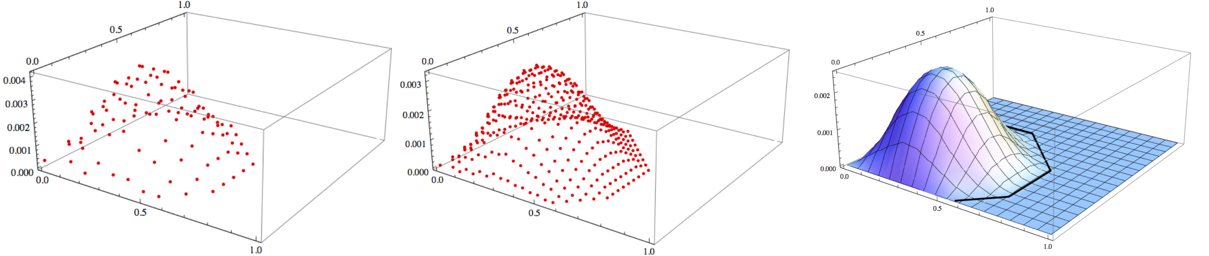
(a)

(b)

(c)

Figure 6.1: Illustration of the semiclassical limit of the Kronecker coefficients. (a) and (b) Suitably rescaled Kronecker coefficients for the mixed-state quantum marginal problem of two qubits with global spectrum $\vec{\lambda}_{AB}=(4/7,2/7,1/7,0)$ and $k=28$ and $56$ boxes (computed with the algorithm described in Section 6.5). (c) The limiting distribution (6.21), whose support is the moment polytope cut out by Bravyi’s inequalities (3.3).

We conclude with an amusing application of (6.24). Consider $\mathcal{H}=\mathbbm{C}^{a}\otimes\mathbbm{C}^{b}$ with $a\leq b$. Recall that Schur–Weyl duality implies that we have the decomposition (2.25),

$$\operatorname{Sym}^{k}(\mathbbm{C}^{a}\otimes\mathbbm{C}^{b})=\bigoplus_{\alpha\vdash_{a}k}V^{a}_{\alpha}\otimes V^{b}_{\alpha}.$$

Restricting to the action of $K=\operatorname{SU}(a)$ on the first tensor factor, we find that

$$\mu_{K,\mathbbm{P}(\mathcal{H})}=\operatorname*{w-lim}_{k\rightarrow\infty}\frac{1}{k^{ab-1-\binom{a}{2}}}\sum_{\alpha\vdash_{a}k}\dim V^{b}_{\alpha}\,\delta_{\alpha/k}.$$

For large $k$, it follows readily from Weyl’s dimension formula (6.14) that

$$\frac{\dim V^{b}_{\alpha}}{k^{a(b-a)+\binom{a}{2}}}\sim\frac{1}{Z}\left(\prod_{i=1}^{a}\left(\alpha_{i}/k\right)^{b-a}\right)p_{a}\left(\alpha/k\right)$$

for some constant $Z>0$. Together with (6.24), we recover (5.25), the formula for the density of the eigenvalue distribution of $\rho_{A}$ for a random bipartite pure state.

Order of Growth and Geometric Complexity Theory

We now consider general projective subvarieties $\mathbbm{X}\subseteq\mathbbm{P}(\mathcal{H})$. In the following, we study the exponent $d_{K,\mathbbm{X}}$ in the definition of the measure (6.21) more carefully and illustrate its implications in the context of geometric complexity theory. We will write $f\sim g$ for the asymptotic equivalence $\lim_{k\rightarrow\infty}f(k)/g(k)=1$.

Lemma .

The exponent $d_{K,\mathbbm{X}}$ is equal to $\dim\mathbbm{X}-R_{\mathbbm{X}}$, where

$$R_{\mathbbm{X}}:=\#\{\alpha\in R_{K,+}:(\lambda,H_{\alpha})>0\text{ for some }\lambda\in\Delta_{K}(\mathbbm{X})\}$$

is the number of positive roots that are not orthogonal to all points on the moment polytope (we write $H_{\alpha}\not\perp\Delta_{K}(\mathbbm{X})$).

Proof.

By the Hilbert–Serre theorem, the function $k\mapsto\dim R_{k}(\mathbbm{X})$ is a polynomial of degree $\dim\mathbbm{X}$ for large $k$ [Har77, Theorem I.7.5]. Hence there exists a constant $A>0$ such that

$$A\,k^{\dim\mathbbm{X}}\sim\dim R_{k}(\mathbbm{X})$$

$$=\leavevmode\nobreak\ \sum_{\mathclap{\lambda\in\Lambda^{*}_{K,+}}}m_{K,R_{k}(\mathbbm{X})}(\lambda)\,\dim V_{K,\lambda}$$

$$=\leavevmode\nobreak\ \sum_{\mathclap{\lambda\in\Delta_{K}(\mathbbm{X})\cap\frac{1}{k}\Lambda^{*}_{K,+}}}m_{K,R_{k}(\mathbbm{X})}(k\lambda)\,\dim V_{K,k\lambda},$$

where for the last equality we have used (6.2). By the Weyl dimension formula (6.14),

$$\dim V_{K,k\lambda}=\prod_{\mathclap{\alpha\in R_{K,+}}}\frac{(k\lambda+\rho_{K},H_{\alpha})}{(\rho_{K},H_{\alpha})}=\underbrace{\left(\leavevmode\nobreak\ \leavevmode\nobreak\ \leavevmode\nobreak\ \leavevmode\nobreak\ \leavevmode\nobreak\ \leavevmode\nobreak\ \prod_{\mathclap{\begin{subarray}{c}\alpha\in R_{K,+}\\ H_{\alpha}\not\perp\Delta_{K}(\mathbbm{X})\end{subarray}}}\leavevmode\nobreak\ \frac{(\lambda,H_{\alpha})}{(\rho_{K},H_{\alpha})}\right)}_{=:p(\lambda)}k^{R_{\mathbbm{X}}}+O(k^{R_{\mathbbm{X}}-1})$$

for the representations that occur in $R(\mathbbm{X})$. The coefficient $p(\lambda)$ of $k^{R_{\mathbbm{X}}}$ is a polynomial function in $\lambda$. We may therefore find a constant $C>0$ such that $\dim V_{K,k\lambda}\leq Ck^{R_{\mathbbm{X}}}$ for all $\lambda\in\Delta_{K}(\mathbbm{X})\cap\frac{1}{k}\Lambda^{*}_{K,+}$. It follows that

$$\sum_{\mathclap{\lambda\in\Delta_{K}(\mathbbm{X})\cap\frac{1}{k}\Lambda^{*}_{K,+}}}m_{K,R_{k}(\mathbbm{X})}(k\lambda)\,\dim V_{K,k\lambda}$$

$$\leq\; Ck^{R_{\mathbbm{X}}}\sum_{\mathclap{\lambda\in\Delta_{K}(\mathbbm{X})\cap\frac{1}{k}\Lambda^{*}_{K,+}}}m_{K,R_{k}(\mathbbm{X})}(k\lambda)$$

$$\sim\; Ck^{R_{\mathbbm{X}}+d_{K,\mathbbm{X}}}\int_{\Delta_{K}(\mathbbm{X})}d\nu_{K,\mathbbm{X}}$$

since the measure $\nu_{K,\mathbbm{X}}$ has non-zero volume. Thus we find that $\dim\mathbbm{X}\leq R_{\mathbbm{X}}+d_{K,\mathbbm{X}}$.

On the other hand, since $\nu_{K,\mathbbm{X}}$ is Lebesgue-absolutely continuous with respect to Lebesgue measure on the moment polytope, we may find a compact set $\Delta$ contained in its relative interior which has positive measure with respect to $\nu_{K,\mathbbm{X}}$. We claim that $p(\lambda)$ is strictly positive for all $\lambda$ contained in the relative interior of the moment polytope. To see this, observe that for all positive roots $\alpha$ with $H_{\alpha}\not\perp\Delta_{K}(\mathbbm{X})$ there exists by definition some $\mu\in\Delta_{K}(\mathbbm{X})$ such that $(H_{\alpha},\mu)>0$; since we can always write $\lambda$ as a proper convex combination of $\mu$ and some other point $\mu^{\prime}\in\Delta_{K}(\mathbbm{X})$, it follows that $(\lambda,H_{\alpha})>0$. This implies that on the compact set $\Delta$ we can bound $p(\lambda)$ from below by a positive constant. Thus there exists a constant $D>0$ (depending on $\Delta$) such that $\dim V_{K,k\lambda}\geq D\,k^{R_{\mathbbm{X}}}$ for all $\lambda\in\Delta\cap\frac{1}{k}\Lambda^{*}_{K,+}$. Consequently,

$$\sum_{\mathclap{\lambda\in\Delta_{K}(\mathbbm{X})\cap\frac{1}{k}\Lambda^{*}_{K,+}}}m_{K,R_{k}(\mathbbm{X})}(k\lambda)\,\dim V_{K,k\lambda}$$

$$\geq\; D\,k^{R_{\mathbbm{X}}}\sum_{\mathclap{\lambda\in\Delta\cap\frac{1}{k}\Lambda^{*}_{K,+}}}m_{K,R_{k}(\mathbbm{X})}(k\lambda)$$

$$\sim\; D\,k^{R_{\mathbbm{X}}+d_{K,\mathbbm{X}}}\int_{\Delta}d\nu_{K,\mathbbm{X}}.$$

Since $\Delta$ has positive measure, we may also conclude that $\dim\mathbbm{X}\geq R_{\mathbbm{X}}+d_{K,\mathbbm{X}}$. Thus we have equality. ∎

Let us now elaborate on the applicability of the multiplicity measures (6.21) for finding new obstructions in geometric complexity theory. For this, we consider a pair of projective subvarieties $\mathbbm{X}$ and $\mathbbm{Y}$ with $\dim\mathbbm{X}<\dim\mathbbm{Y}$, as is the case for the orbit closures of relevance to geometric complexity theory [BLMW11, BI11].

Lemma .

Let $\Delta_{K}(\mathbbm{X})\subseteq\Delta_{K}(\mathbbm{Y})$ and $R_{\mathbbm{X}}<R_{\mathbbm{Y}}$. Then, $\dim\Delta_{K}(\mathbbm{X})<\dim\Delta_{K}(\mathbbm{Y})$.

Proof.

Note that we have

$$\dim\Delta_{K}(\mathbbm{X})=\dim\operatorname{aff}\Delta_{K}(\mathbbm{X})\leq\dim\operatorname{aff}\Delta_{K}(\mathbbm{Y})=\dim\Delta_{K}(\mathbbm{Y}),$$

with equality if and only if the two affine hulls are equal. By assumption there exists a positive root $\alpha\in R_{K,+}$ such that $H_{\alpha}$ is orthogonal to all points in $\Delta_{K}(\mathbbm{X})$ (i.e., $(\lambda,H_{\alpha})=0$ for all $\lambda\in\Delta_{K}(\mathbbm{X})$), but not to all points in $\Delta_{K}(\mathbbm{Y})$. Then $H_{\alpha}$ is also orthogonal to all points in the affine hull of $\Delta_{K}(\mathbbm{X})$, but not to all points in the affine hull of $\Delta_{K}(\mathbbm{Y})$. Since $\Delta_{K}(\mathbbm{X})\subseteq\Delta_{K}(\mathbbm{Y})$ by assumption, it follows that $\operatorname{aff}\Delta_{K}(\mathbbm{X})\subsetneq\operatorname{aff}\Delta_{K}(\mathbbm{Y})$, and hence that $\dim\Delta_{K}(\mathbbm{X})<\dim\Delta_{K}(\mathbbm{Y})$. ∎

Lemma .

Let $\dim\Delta_{K}(\mathbbm{X})<\dim\Delta_{K}(\mathbbm{Y})$. Then, $\mathbbm{X}\subseteq\mathbbm{Y}$ implies that $d_{K,\mathbbm{X}}<d_{K,\mathbbm{Y}}$.

Proof.

If $\mathbbm{X}\subseteq\mathbbm{Y}$ then it is immediate from (6.4) and the definition of the measures (6.21) that $d_{K,\mathbbm{X}}\leq d_{K,\mathbbm{Y}}$. Let us suppose for a moment that in fact $d_{K,\mathbbm{X}}=d_{K,\mathbbm{Y}}$. Then (6.4) would imply that

$$\int d\nu_{K,\mathbbm{X}}\,g\leq\int d\nu_{K,\mathbbm{Y}}\,g$$

for any non-negative test function $g$. In particular, this inequality would hold for the indicator function of $\Delta_{K}(\mathbbm{X})$, so that

$$0<\int_{\Delta_{K}(\mathbbm{X})}d\nu_{K,\mathbbm{X}}\leq\int_{\Delta_{K}(\mathbbm{X})}d\nu_{K,\mathbbm{Y}}.$$

But this is clearly absurd—since $\nu_{K,\mathbbm{Y}}$ is absolutely continuous with respect to Lebesgue measure on its moment polytope $\Delta_{K}(\mathbbm{Y})$, the assumption implies that $\Delta_{K}(\mathbbm{X})$ is a set of measure zero for $\nu_{K,\mathbbm{Y}}$; thus the right-hand side integral is zero. ∎

Corollary .

Let $\dim\mathbbm{X}<\dim\mathbbm{Y}$. Then, $\mathbbm{X}\subseteq\mathbbm{Y}$ implies $d_{K,\mathbbm{X}}<d_{K,\mathbbm{Y}}$.

Proof.

Clearly, $\mathbbm{X}\subseteq\mathbbm{Y}$ implies that $\Delta_{K}(\mathbbm{X})\subseteq\Delta_{K}(\mathbbm{Y})$ and $R_{\mathbbm{X}}\leq R_{\mathbbm{Y}}$. If $R_{\mathbbm{X}}=R_{\mathbbm{Y}}$ then the assertion follows directly from Section 6.6, since then

$$d_{K,\mathbbm{X}}=\dim\mathbbm{X}-R_{\mathbbm{X}}<\dim\mathbbm{Y}-R_{\mathbbm{Y}}=d_{K,\mathbbm{Y}}.$$

Otherwise, if $R_{\mathbbm{X}}<R_{\mathbbm{Y}}$ then Section 6.6 and Section 6.6 together imply that $d_{K,\mathbbm{X}}<d_{K,\mathbbm{Y}}$. ∎

As we had explained in the introduction, the significance of Section 6.6 is that the multiplicity measures do not directly lead to a new criterion for obstructions that goes beyond what is provided by the moment polytope. From a conceptual point of view, the exponents $d_{K,\mathbbm{X}}$ and $d_{K,\mathbbm{Y}}$ each capture the order of growth, while the densities of the measures $\nu_{K,\mathbbm{X}}$ and $\nu_{K,\mathbbm{Y}}$ encode (smoothed versions) of the corresponding leading-order coefficients—but the latter are incomparable if the orders of growth differ!

6.7 Discussion

In a recent preprint, our algorithm for computing Kronecker coefficients has been analyzed in some detail and it has also been shown that it is possible to decide positivity in linear time for Young diagrams of bounded height [PP14]. The problem of efficiently deciding the positivity of Kronecker coefficients for general Young diagrams, though, is still wide open, partly because we do not know of an effective combinatorial description akin to the honeycomb model for the Littlewood–Richardson coefficients [KT99].

In the past chapters, we have studied the one-body reduced density matrix in quantum mechanics from a variety of perspectives. In Chapter 3, we gave a new solution to the one-body quantum marginal in terms of “Ressayre-type inequalities”. In Chapter 4, we studied multipartite entanglement from the perspective of the one-body marginals. In Chapter 5, we showed how the joint distribution of the local eigenvalues can be computed by reducing to the distribution of diagonal entries; the discrete analogue of this reduction leads to an efficient algorithm for the subgroup restriction problem as we have seen in this Chapter 6. Common to all our results is the remarkable role played by the maximal unipotent subgroups and the interplay between highest weights and weights, which in each case allowed us to reduce from a non-Abelian quantum-mechanical problem to an Abelian one, and thus in essence to the classical combinatorics of weights.

Chapter 7 The Search for Further Entropy Inequalities

In the second part of this thesis, we go beyond the study of one-body reduced density matrices and consider general quantum marginals. Motivated by the fundamental role of entropy in physics and information theory, we start by introducing in this chapter the problem of determining the linear inequalities that constrain the von Neumann entropy of the marginals of a multipartite quantum state [Pip03]. The strong subadditivity of the von Neumann entropy is perhaps the most important such inequality [LR73], and an indispensable tool in quantum statistical physics and quantum information theory [OP93]. The discovery of any further entropy inequality would be considered a major breakthrough, and it would shed further light on the general quantum marginal problem.

The following introduction is partially adapted from [GW13]. We refer to [CT06, Yeu02] and [NC04] for comprehensive introductions to classical and quantum entropy.

The Classical Entropy Cone

Let us first consider the classical situation.

Definition .

The Shannon entropy of a random variable $X$ with finitely many outcomes is given by

$$H(X)=H(p)=-\sum_{x}p_{x}\log p_{x}\geq 0,$$

where $p=(p_{x})$ is the probability distribution of $X$ (i.e., $p_{x}$ is the probability of an outcome $x$).

Given a collection of random variables $X_{1},\dots,X_{n}$ defined on a common probability space, we can then consider the Shannon entropy $H(X_{I})$ of any non-empty subset $X_{I}=(X_{i})_{i\in I}$ of the variables. These entropies are not independent: For example, monotonicity asserts that the Shannon entropy can never decrease if more random variables are taken into account:

$$H(X_{I\cup J})-H(X_{I})\geq 0$$ (7.1)

A second example is the strong subadditivity of the Shannon entropy:

$$H(X_{I})+H(X_{J})-H(X_{I\cap J})-H(X_{I\cup J})\geq 0$$ (7.2)

Equivalently, the conditional entropy and the conditional mutual information are always non-negative. To study the entropies of subsystems systematically, we define the classical entropy region

$$\mathcal{C}_{n}:=\{(H(X_{I}))_{\emptyset\neq I\subseteq\{1,\dots,n\}}:\; X_{1},\dots,X_{n}\text{ random variables}$$

$$\text{with finitely many outcomes}\}\subseteq\mathbbm{R}^{2^{n}-1}.$$

In general, the set $\mathcal{C}_{n}$ has a complicated geometrical structure [ZY97]. However, its closure $\overline{\mathcal{C}_{n}}$ is a convex cone [ZY97], which we call the classical entropy cone. Like any closed convex cone, $\overline{\mathcal{C}_{n}}$ can be described by linear inequalities. To see this, consider the dual cone

$$\overline{\mathcal{C}_{n}}^{*}=\mathcal{C}_{n}^{*}=\{(\nu_{I})\in\mathbbm{R}^{2^{n}-1}:\sum_{I}\nu_{I}H(X_{I})\geq 0\quad\forall X_{1},\dots,X_{n}\}.$$

Each element $(\nu_{I})\in\mathcal{C}_{n}^{*}$ can be identified with an entropy inequality $\sum_{I}\nu_{I}H(X_{I})\geq 0$ that is satisfied by the Shannon entropy. The bipolar theorem now asserts that the bidual cone $\mathcal{C}_{n}^{**}$ is equal to $\overline{\mathcal{C}_{n}}$ (e.g., [Roc72]). Thus the set of entropy inequalities (or even just its extreme rays) determines the classical entropy region up to closure [Pip86]. Matús̆ has shown that the classical entropy region contains the relative interior of the classical entropy cone, so that $\operatorname{relint}\overline{\mathcal{C}_{n}}\subseteq\mathcal{C}_{n}\subseteq\overline{\mathcal{C}_{n}}$.

Monotonicity (7.1) and strong subadditivity (7.2) together span the polyhedral cone of entropy inequalities of Shannon-type. For any given candidate inequality it can be automatically checked by using linear programming if it is an entropy inequality of Shannon-type [YY, Yeu97]. For a long time, these were the only known inequalities. Equivalently, it was not known if monotonicity and strong subadditivity were the only constraints on a non-negative vector $(h_{I})$ to be approximable by the Shannon entropies of random variables.

In the seminal work [ZY98], Zhang and Yeung have shown that for $n\geq 4$ random variables there exist entropy inequalities that are not of Shannon-type. In particular, they have proved that

$$2I(X_{3}:X_{4})\leq I(X_{1}:X_{2})+I(X_{1}:X_{34})+3I(X_{3}:X_{4}|X_{1})+I(X_{3}:X_{4}|X_{2})$$ (7.3)

is a linear entropy inequality that is not of Shannon-type. Here, $I(X_{I}:X_{J})=S(X_{I})+S(X_{J})-S(X_{I\cup J})$ and $I(X_{I}:X_{J}|X_{K}):=H(X_{I\cup K})+H(X_{J\cup K})-H(X_{I\cup J\cup K})-H(X_{K})$ are the Shannon (conditional) mutual information. In fact, there are infinitely many independent inequalities that are not of Shannon-type. Thus the classical entropy cone $\mathcal{C}_{n}$ is not polyhedral for $n\geq 4$ [Mat07, DFZ11]. Its general structure is still only poorly understood, and any improved understanding should have direct applications to network information theory [Yeu02, SJ13].

The Quantum Entropy Cone

We now consider the situation in quantum mechanics. Here, the natural analogue of the Shannon entropy is the von Neumann entropy:

Definition .

The von Neumann entropy of a density matrix $\rho$ on a finite-dimensional Hilbert space is given by

$$S(\rho)=-\operatorname{tr}\rho\log\rho\geq 0.$$

By the spectral theorem, the von Neumann entropy $S(\rho)$ is equal to $H(\vec{\lambda})$, the Shannon entropy of the spectrum $\vec{\lambda}$ of $\rho$, which is a probability distribution. It is a concave function of $\rho$.

Now let $\rho$ be a density matrix describing the state of a quantum system of $n$ distinguishable particles with tensor-product Hilbert space $\mathcal{H}=\bigotimes_{i=1}^{n}\mathcal{H}_{i}$. The state of any subset $I\subseteq\{1,\dots,n\}$ of the particles is described by the reduced density matrix $\rho_{I}=\operatorname{tr}_{I^{c}}\rho$ formed by tracing out the Hilbert space of the other particles. We define the quantum entropy region to be [Pip03]

$$\mathcal{Q}_{n}:=\{(S(\rho_{I}))_{\emptyset\neq I\subseteq\{1,\dots,n\}}\;:\; \rho\text{ density matrix on an $n$-fold tensor product}$$

$$\text{of finite-dimensional Hilbert spaces}\}\subseteq\mathbbm{R}^{2^{n}-1}.$$

Clearly, $\mathcal{Q}_{n}\supseteq\mathcal{C}_{n}$, since any joint probability distribution can be considered as a multipartite density matrix. In general, $\mathcal{Q}_{n}$ has a complex structure and in particular is neither closed nor convex [LW05b]. But its closure is again a convex cone, called the quantum entropy cone. We recall a proof of this important fact:

Lemma ([Pip03]).

The quantum entropy cone $\overline{\mathcal{Q}_{n}}$ is indeed a convex cone.

Proof.

(1) We first show that $\mathcal{Q}_{n}+\mathcal{Q}_{n}\subseteq\mathcal{Q}_{n}$: Let $\rho$, $\rho^{\prime}$ be quantum states on $\bigotimes_{i=1}^{n}\mathcal{H}_{i}$ and $\bigotimes_{i=1}^{n}\mathcal{H}^{\prime}_{i}$, respectively. Then $\rho^{\prime\prime}:=\rho\otimes\rho^{\prime}$ is a quantum state on $\bigotimes_{i=1}^{n}\mathcal{H}_{i}\otimes\mathcal{H}^{\prime}_{i}$, and $\rho^{\prime\prime}_{I}=\rho_{I}\otimes\rho^{\prime}_{I}$ for each subset $I\subseteq\{1,\dots,n\}$. By additivity of the von Neumann entropy, $S(\rho^{\prime\prime}_{I})=S(\rho_{I})+S(\rho^{\prime}_{I})$, which shows the claim.

(2) We now show that $\lambda\mathcal{Q}_{n}\subseteq\overline{\mathcal{Q}_{n}}$ for all $\lambda\geq 0$: For this, let $\rho$ be a quantum state on $\bigotimes_{i=1}^{n}\mathcal{H}_{i}$. Let $p\in[0,1]$ and $k\in\mathbbm{N}_{>0}$ and consider the quantum state $\rho^{\prime}:=(1-p)\lvert 0\rangle\langle 0\rvert^{\otimes n}+p\rho^{\otimes k}$ on $\bigotimes_{i=1}^{n}\left(\mathbbm{C}\ket{0}\oplus\mathcal{H}_{i}^{\otimes k}\right)$. Then, $\rho^{\prime}_{I}=(1-p)\lvert 0\rangle\langle 0\rvert^{\otimes I}+p\rho_{I}^{\otimes k}$, so that

$$S(\rho^{\prime}_{I})=h(p)+pkS(\rho_{I}),$$

where $h(p)=-p\log p-(1-p)\log(1-p)$ is the binary entropy function. Let $\varepsilon>0$. Since $h(p)$ is continuous and $h(0)=0$, we may choose $k$ large enough such that $h(p)\leq\varepsilon$ for $p=\lambda/k$, and hence

$$\lvert S(\rho^{\prime}_{I})-\lambda S(\rho_{I})\rvert\leq\varepsilon.$$

Since $\varepsilon>0$ was arbitrary, we may conclude that $(\lambda S(\rho_{I}))\in\overline{\mathcal{Q}_{n}}$. This establishes the second claim.

By taking limits, points (1) and (2) together imply that $\overline{\mathcal{Q}_{n}}$ is a convex cone. ∎

The most immediate difference to the classical case is that the von Neumann entropy is no longer monotonic: Global quantum states can exhibit less entropy than their reductions (a signature of entanglement), which also shows that $\mathcal{Q}_{n}\supsetneq\mathcal{C}_{n}$. Instead, the von Neumann entropy satisfies weak monotonicity:

$$S(\rho_{I})+S(\rho_{J})-S(\rho_{I\setminus J})-S(\rho_{J\setminus I})\geq 0$$ (7.4)

Strong subadditivity, however, famously remains valid for quantum entropies [LR73]:

$$S(\rho_{I})+S(\rho_{J})-S(\rho_{I\cap J})-S(\rho_{I\cup J})\geq 0$$ (7.5)

In fact, (7.4) and (7.5) are easily shown to be equivalent by the process of purification [Lie75]. Since purification is a non-linear construction, this does not imply equivalence on the level of the entropy regions; but see the discussion in [LMRW13].

Just as in the classical case, it is of fundamental interest to determine the linear inequalities satisfied by the von Neumann entropies $S(\rho_{I})$ of subsystems. In fact, it is a major open problem to decide if there are any further entropy inequalities besides weak monotonicity and strong subadditivity [Pip03]. Let us describe some partial progress from the literature: For vectors $(s_{I})\in\mathbbm{R}^{2^{n}-1}$ that are permutation-invariant under relabeling of the subsystems, it has been shown that $(s_{I})\in\overline{\mathcal{Q}_{n}}$ if and only if weak monotonicity and strong subadditivity are satisfied [Pip03]. In [LW05b, CLW12] a class of so-called constrained inequalities has been established, which in particular showed that $\mathcal{Q}_{n}\subsetneq\overline{\mathcal{Q}_{n}}$. We also refer to [Ibi07] for numerical evidence that the Zhang–Yeung inequality (7.3) might also hold for the von Neumann entropy.

Balanced Entropy Inequalities

Instead of directly determining the quantum entropy cone, it is natural to approach the problem by asking which of the classical entropy inequalities might continue to hold for the von Neumann entropy. Since the latter is no longer monotonic, we need to identify those classical entropy inequalities which do not “involve” monotonicity. An interesting class of entropy inequalities introduced by Chan does precisely that:

Definition .

An entropy inequality $\sum_{I}\nu_{I}H(X_{I})\geq 0$ or $\sum_{I}\nu_{I}S(\rho_{I})\geq 0$ is called balanced [Cha03] (also correlative [Han75]) if

$$\sum_{I\ni i}\nu_{I}=0\quad(\forall i=1,\dots,n).$$

For example, strong subadditivity is balanced, while monotonicity is not. Chan has shown that the classical entropy cone is determined by the set of balanced entropy inequalities together with monotonicity. More precisely, he has proved that any Shannon entropy inequality can be decomposed uniquely into the form

$$\sum_{I}\nu_{I}H(X_{I})+\sum_{i=1}^{n}r_{i}H(X_{i}|X_{i^{c}})\geq 0,$$ (7.6)

where the left-hand side is a balanced entropy inequality and the right-hand side a conic combination of conditional entropies, i.e. all $r_{i}\geq 0$ [Cha03]. In other words, the dual cone $\mathcal{C}^{*}_{n}$ of Shannon entropy inequalities is a direct sum of the cone of balanced entropy inequalities and the cone spanned by monotonicity (7.1). It is thus natural to consider the following problem.

Problem .

Which balanced Shannon entropy inequalities also hold true for the von Neumann entropy?

We remark that the Zhang–Yeung inequality (7.3) as well as the infinite families in [Mat07, DFZ11] are balanced, since they are linear combinations of conditional mutual informations. On the other hand, we note that there are unbalanced entropy inequalities that hold for the von Neumann entropy, e.g. weak monotonicity. It can be argued that there is no direct quantum counterpart of the decomposition (7.6) [Maj14], which perhaps makes it unlikely that the problem of determining all linear entropy inequalities satisfied by the von Neumann entropy can be reduced to Chapter 7.

Discussion

We conclude this introduction by mentioning some related avenues of investigation. Entropic constraints are of interest not only for the Shannon and von Neumann entropy, but also for other kinds of entropies, e.g. differential entropies [Cha03] and Rényi entropies [LMW13, CHLW14]. Another interesting direction is to relax the notion of subsystems beyond the tensor-product case. Instead of only considering partial traces over the factors of a tensor-product Hilbert space, we may consider marginals with respect to more general subalgebras of observables [OP93]. This leads directly to the study of entropic uncertainty relations [BCC⁺10, MU88], entropy power inequalities [KS14], and entropy in space-time and might thus serve as a unifying framework for studying entropy in general quantum systems.

Chapter 8 Entropy Inequalities from Phase Space

In this chapter we study the entropy inequalities satisfied by two classes of quantum states—namely, stabilizer states and Gaussian states (the latter can be seen as continuous-variable counterparts of the former). Both classes of states can exhibit intrinsically quantum features, such as multi-particle entanglement, but they possess enough structure to allow for a concise and computationally efficient description and so have proven to be extremely useful in quantum information theory and beyond. For example, the stabilizer formalism is a basic tool for constructing quantum error-correcting codes, while Gaussian states and transformations are routinely used in quantum optics (see, e.g., [NC04, WPGP⁺12]). Quantum phase-space methods have been built around both classes of states, and it is this point of view we will exploit here.

The results in this chapter have been obtained in collaboration with David Gross, and they have appeared in [GW13].

8.1 Summary of Results

The starting point for our work is the Wigner function, which for Gaussian states as well as for stabilizer states in odd dimensions $d$ is a bona fide probability distribution on the classical phase space (the case of even $d$ requires some more care, see Theorem 8.2 below). For $n$ bosonic modes, this phase space is given by $\mathbbm{R}^{2n}$, while for $n$ systems of local dimension $d$, it is the finite group $\mathbbm{Z}_{d}^{2n}$. In both cases, it is the direct sum of the single-particle or single-mode phase spaces. In Sections 8.2 and 8.3 we give a self-contained account of stabilizer states in the discrete phase-space formalism. We may thus define random variables $X_{1},\dots,X_{n}$ on the phase space, jointly distributed according to the Wigner function of the given quantum state $\rho$. Here, $X_{i}$ denotes the component in the phase space of the $i$-th particle or mode. The random variables $X_{1},\dots,X_{n}$ constitute our classical model. This construction is compatible with reduction: The marginal probability distribution of a subset of variables $X_{I}=(X_{i})_{i\in I}$ is given precisely by the Wigner function of the reduced density matrix $\rho_{I}$.

Our crucial observation then is that certain quantum entropies are simple functions of corresponding classical entropies. More precisely, in the case of stabilizer states (Section 8.4), we find that

$$S(\rho_{I})=H(X_{I})-\lvert I\rvert\log(d).$$ (8.1)

Therefore, if $\sum_{I}\nu_{I}H(X_{I})\geq 0$ is a balanced entropy inequality satisfied by the Shannon entropies of the random variables $X_{I}$ then the same inequality is also satisfied by the von Neumann entropies of the quantum states $\rho_{I}$:

$$\sum_{I}\nu_{I}S(\rho_{I})=\sum_{I}\nu_{I}H(X_{I})-\underbrace{\sum_{I}\nu_{I}\lvert I\rvert}_{=0}\log(d)\geq 0$$

In particular, the von Neumann entropy of stabilizer states respects all balanced Shannon entropy inequalities, such as the inequalities of non-Shannon type found in [ZY98, Mat07, DFZ11]. This completely solves Chapter 7 for the class of stabilizer states.

Our construction can also be understood in the group-theoretical framework of [CY02]. Here it is well-known that there are inequalities for the Shannon entropy which do not hold for arbitrary random variables, but only for random variables constructed from certain classes of subgroups [LC07]. By analyzing the construction above, we show that the von Neumann entropy for stabilizer states similarly respects a further entropy inequality which does not hold for arbitrary random variables (and hence quantum states)—namely the Ingleton inequality [LC07], which is the balanced inequality

$$I_{\rho}(I:J|K)+I_{\rho}(I:J|L)+I_{\rho}(K:L)-I_{\rho}(I:J)\geq 0.$$ (8.2)

Here, $I_{\rho}(I:J)=S(\rho_{I})+S(\rho_{J})-S(\rho_{I\cup J})$ and $I_{\rho}(I:J|K)=S(\rho_{I\cup K})+S(\rho_{J\cup K})-S(\rho_{K})-S(\rho_{I\cup J\cup K})$ are the quantum (conditional) mutual information.

We find it instructive to understand how the above classical model manages to respect monotonicity (7.1), while the quantum state may violate it. For example, since stabilizer states can be entangled (even maximally so, see Section 8.3 below), $S(\rho_{1})=S(\rho_{2})=1$ and $S(\rho_{12})=0$ are perfectly valid entropies of a stabilizer state which certainly violate monotonicity. Equation (8.1) states that the classical model is more highly mixed than the quantum one, in the sense that the entropy associated with a subset $I$ is higher by an amount of $\lvert I\rvert$ $d$its. That is precisely the maximal amount by which quantum mechanics can violate monotonicity.

In the case of Gaussian states (Section 8.5), the random variables $X_{1},\dots,X_{n}$ have a multivariate normal distribution on $\mathbbm{R}^{2n}$, and we show that

$$S_{2}(\rho_{I})=h_{\alpha}(X_{I})-\lvert I\rvert\left(\log\pi-\frac{\log\alpha}{1-\alpha}\right),$$

where $S_{2}(\rho)=-\log\operatorname{tr}\rho^{2}$ is the quantum Rényi-2 entropy; $h_{\alpha}$ is the differential Rényi-$\alpha$ entropy, defined by $h_{\alpha}(X)=(1-\alpha)^{-1}\log\int p(x)^{\alpha}dx$ for any positive $\alpha\neq 1$, with $p(x)$ the probability density of the random variable $X$ with respect to Lebesgue measure. In the limiting case $\alpha\rightarrow 1$, we recover a formula involving the differential Shannon entropy $h(X)=-\int p(x)\log p(x)$, which has previously appeared in [AGS12], attributed to Stratonovich:

$$S_{2}(\rho_{I})=h(X_{I})-\lvert I\rvert\log(\pi e)$$

Thus, Rényi-2 entropies of Gaussian states respect all balanced entropy inequalities that hold for the Shannon entropies of multivariate normal distributions. The latter have been investigated in the literature (see, e.g., [HS07, SH11]).

In Section 8.6 we discuss the relation between our results for stabilizer states and Gaussian states and point towards further avenues of investigations.

Related Work

Independently of the work presented in this chapter, Linden, Ruskai, and Winter have published an analysis of the entropy cone generated by stabilizer states [LMRW13]. Their methods – focusing on group-theoretical constructions – are conceptually complementary to our phase-space approach. [LMRW13] contains a complete characterization of the entropy cone generated by four-party stabilizer states. The paper also lists further examples of inequalities which, like the Ingleton Inequality, are respected by stabilizer states, even though there are classical distributions violating it. While not originally stated explicitly, their results also imply that all balanced inequalities remain valid for stabilizer states (see Theorem 11 in [LMRW13] and discussion thereafter).

8.2 Discrete Phase Space

In this section, we present a self-contained account of Weyl operators and stabilizer states in the discrete phase-space picture. This section does not contain original results. All statements could be found in some form in [Got96, App05, Gro06, Bea13, KG13], albeit not in a unified language.

Discrete Symplectic Geometry

Let $d>1$ be an integer and let $\mathbbm{Z}_{d}=\mathbbm{Z}/d\mathbbm{Z}$ be the ring of (congruence classes of) integers modulo $d$. The discrete phase space for $n$ particles with local dimension $d$ is by definition $V=\bigoplus_{i=1}^{n}V_{i}=\mathbbm{Z}_{d}^{2n}$, the free $\mathbbm{Z}_{d}$-module of rank $2n$. Given a point $v\in V$, we write $v_{i}=(p_{i},q_{i})\in V_{i}=\mathbbm{Z}_{d}^{2}$ for its components. Consider the bilinear form $\omega\colon V\times V\rightarrow\mathbbm{Z}_{d}$ defined by

$$\omega(v,v^{\prime})=\sum_{i=1}^{n}p_{i}q_{i}^{\prime}-q_{i}p_{i}^{\prime}.$$

It is non-degenerate and totally isotropic, i.e. $\omega(v,v)=0$ for all $v\in V$. If $d$ is prime then $V$ is simply a symplectic vector space over the finite field $\mathbbm{F}_{d}=\mathbbm{Z}_{d}$. We will also in the general case refer to $\omega$ as the symplectic form.

A character of a finite Abelian group $G$ is a group homomorphism $G\rightarrow\operatorname{U}(1)$. Denote by $\widehat{G}$ the set of characters, which is again an Abelian group with the operation of pointwise multiplication. It is called the (Pontryagin) dual of $G$. It is well-known that $G\cong\widehat{G}$, although not canonically. For the cyclic group $G=\mathbbm{Z}_{d}$, all characters are powers of $\chi_{d}(x)=e^{\frac{2\pi\mathrm{i}}{d}x}$.

Lemma .

The characters of the additive group of the phase space $V$ are $\widehat{V}=\{\chi_{d}(\omega(v,-)):v\in V\}\cong V$.

Proof.

By injectivity of $\chi_{d}\colon\mathbbm{Z}_{d}\rightarrow\operatorname{U}(1)$ and non-degeneracy of the symplectic form, each $v$ determines a different character. Thus we have found all $\lvert\widehat{V}\rvert=\lvert V\rvert$ many characters. ∎

The symplectic complement of a submodule $M\subseteq V$ is the submodule $M^{\omega}=\{v\in V:\omega(v,m)=0\;(\forall m\in M)\}$. In the case of prime $d$, it is well-known that $\dim M+\dim M^{\omega}=\dim V$—however, in general the dimension (or rank) might not even be well-defined. Still there is an important analogue that holds in the general case:

Lemma .

$\lvert M\rvert\lvert M^{\omega}\rvert=\lvert V\rvert$.

Proof.

We show that the group homomorphism

$$\Phi\colon M^{\omega}\rightarrow\widehat{V/M},\quad v\mapsto\left([w]\mapsto\chi_{d}(\omega(v,w))\right)$$

is both injective and surjective (it is certainly well-defined). Injectivity follows immediately from the non-degeneracy of the symplectic form. For surjectivity, let $\tau\in\widehat{V/M}$. Then $w\mapsto\tau([w])$ is a character of $V$. By Section 8.2, there exists $v\in V$ such that $\tau([w])=\chi_{d}(\omega(v,w))$. Since $\tau$ vanishes on $M$, $v\in M^{\omega}$. Thus $\Phi$ is an isomorphism, and we find that

$$\lvert M^{\omega}\rvert=\lvert\widehat{V/M}\rvert=\lvert V/M\rvert=\frac{\lvert V\rvert}{\lvert M\rvert}.\qed$$

The following important corollary follows from Section 8.2 and $M\subseteq(M^{\omega})^{\omega}$:

Corollary .

$(M^{\omega})^{\omega}=M$.

We call a submodule $M\subseteq V$ an isotropic submodule if $M\subseteq M^{\omega}$, i.e. if $\omega(m,m^{\prime})=0$ for all $m,m^{\prime}\in M$. Finally consider $V_{I}=\bigoplus_{i\in I}V_{i}$, the phase space of particles $I\subseteq\{1,\dots,n\}$. There is a natural way of restricting a submodule $M$ to $V_{I}$: we set

$$M_{I}:=M\cap V_{I},$$

where $V_{I}$ is identified with a submodule of $V$ in the natural way.

Weyl Representation

Following [App05, Bea13], we first define Weyl operators for general integers $(P,Q)\in\mathbbm{Z}^{2}$, not necessarily in the range $\{0,\dots,d-1\}$. These are the unitaries on $L^{2}(\mathbbm{Z}_{d})\cong\mathbbm{C}^{d}$ given by

$$(W({P,Q})\psi)(x)=\tau_{2d}(-PQ)\,\chi_{d}(Px)\,\psi(x-Q),$$

where $\tau_{2d}(R)=\chi_{2d}((d^{2}+1)R)$. For example, $W({1,0})$ is the $Z$-operator $\ket{x}\mapsto e^{\frac{2\pi\mathrm{i}}{d}x}\ket{x}$, while $W({0,1})$ is the $X$-operator $\ket{x}\mapsto\ket{x+1\pmod{d}}$. By direct computation [Bea13],

$$W({P,Q})W({P^{\prime},Q^{\prime}}) =\tau_{2d}(PQ^{\prime}-QP^{\prime})\,W({P+P^{\prime},Q+Q^{\prime}}),$$ (8.3)

$$W({P,Q})^{-1} =W({P,Q})^{\dagger}=W({-P,-Q}),$$ (8.4)

$$W({P,Q})W({P^{\prime},Q^{\prime}}) =\chi_{d}(PQ^{\prime}-QP^{\prime})\,W({P^{\prime},Q^{\prime}})W({P,Q}).$$ (8.5)

We now introduce the Weyl operators $w(p,q)$ for congruence classes $(p,q)\in\mathbbm{Z}_{d}^{2}$. It is here that the treatment of the odd and the even-dimensional case diverges.

For $d$ odd, $\tau_{2d}(1)=\chi_{d}\big{(}\frac{d^{2}+1}{2}\big{)}$ is a $d$-th root of unity, so that $W(P+d,Q)=W(P,Q+d)=W(P,Q)$. In other words, $W$ is constant on congruence classes modulo $d$, so we can directly define $w(p,q):=W(P,Q)$. In fact, $2^{-1}:=\frac{d^{2}+1}{2}\in\mathbbm{Z}$ is the multiplicative inverse of $2$ modulo $d$, so that

$$(w(p,q)\psi)(x)=\chi_{d}(px-2^{-1}pq)\,\psi(x-q)$$

$$w(v)w(v^{\prime})=\chi_{d}(2^{-1}\omega(v,v^{\prime}))\,w(v+v^{\prime}).$$ (8.6)

For $d$ even, $\tau_{2d}(1)=\chi_{2d}(1)$ is a primitive $2d$-th root of unity (e.g., in the case of qubits $\tau_{2d}(1)=i$). Equation (8.3) then implies that $W(P+d,Q)$ and $W(P,Q+d)$ are either $W(P,Q)$ or $-W(P,Q)$. In order to fix the sign, we choose $w(p,q):=W(P,Q)$ where $(P,Q)$ is the unique preimage in $\{0,\dots,d-1\}^{2}\subseteq\mathbbm{Z}^{2}$. Because $w$ and $W$ differ at most by a phase, (8.3) still implies that $(p,q)\mapsto w(p,q)$ defines a projective representation of the additive structure of the phase space $\mathbbm{Z}_{d}^{2}$.

In both the even and the odd case, it now follows from (8.4) and (8.5) that

$$w(v)^{-1} =w(v)^{\dagger}=\pm w(-v),$$ (8.7)

$$w(v)w(v^{\prime}) =\chi_{d}(\omega(v,v^{\prime}))\,w(v^{\prime})w(v).$$ (8.8)

For $n$-particles, the phase space is the direct sum $V=\bigoplus_{i=1}^{n}V_{i}=\mathbbm{Z}_{d}^{2n}$. We define its Weyl representation on $(\mathbbm{C}^{d})^{\otimes n}$ by the tensor product of the single-particle representations, $w(v)=\bigotimes_{i=1}^{n}w(v_{i})$. In this way, the relations (8.7) and (8.8) continue to hold. Moreover, it is easy to verify that

$$\operatorname{tr}w(v)=d^{n}\,\delta_{v,0}.$$ (8.9)

8.3 Stabilizer States in Phase Space

To define stabilizer states, we start with a stabilizer group $G$, i.e. a finite Abelian group whose elements are scalar multiples of Weyl operators on $(\mathbbm{C}^{d})^{\otimes n}$, such that the only multiple of $\mathbbm{1}=w(0)$ contained in $G$ is $\mathbbm{1}$ itself. With such a group we associate the operator

$$P=\frac{1}{\lvert G\rvert}\sum_{g\in G}g.$$

From the fact that $G$ is a group, we deduce that $P^{2}=P$; since all elements of $G$ are unitaries, $P=P^{\dagger}$; and (8.9) implies that $\operatorname{tr}P=d^{n}/|G|$. Hence $P$ projects onto a $\big{(}d^{n}/|G|\big{)}$-dimensional subspace, called the stabilizer code of $G$. Note that the stabilizer code is the subspace of all vectors that are stabilized by $G$. The corresponding stabilizer state is $\rho=\frac{1}{d^{n}}\sum_{g}g$. We refer to [NC04, §10.5] for an introduction to the stabilizer formalism from the perspective of quantum information theory.

We now prove the central theorem that provides a description of stabilizer states in terms of discrete phase space:

Theorem 8.1 (Stabilizers in phase space).

Let $V=\bigoplus_{i=1}^{n}V_{i}=\mathbbm{Z}^{2n}_{d}$ be the phase space for $n$ particles with local dimension $d$, where $d>1$ is an arbitrary integer. There is a one-to-one correspondence between isotropic submodules $M\subseteq V$ and equivalence classes $[\rho(M)]$ of stabilizer states on $(\mathbbm{C}^{d})^{\otimes n}$ under conjugation with Weyl operators. Moreover,

$$[\rho(M)_{I}] =[\rho(M_{I})],$$ (8.10)

$$S([\rho(M)_{I}]) =\lvert I\rvert\log(d)-\log\ \lvert M_{I}\rvert$$ (8.11)

for all subsets $I\subseteq\{1,\dots,n\}$. If $d$ is odd then there is a canonical element $\rho(M)$ in each equivalence class, given by

$$\rho(M)=\frac{1}{d^{n}}\sum_{m\in M}w(m).$$ (8.12)

It is compatible with reductions, i.e. $\rho(M)_{I}=\rho(M_{I})$.

Proof.

(1) From isotropic submodules to classes of stabilizer states: Let $M\subseteq\mathbbm{Z}_{d}^{2n}$ be an isotropic submodule. Since $M$ is a finite Abelian group, it can be written as a direct sum of cyclic groups, $M\cong\mathbbm{Z}_{d_{1}}\oplus\dots\oplus\mathbbm{Z}_{d_{k}}$. Let $m_{j}\in M$ be a generator of the $j$-th cyclic subgroup. Since $w(m_{j})^{d_{j}}\propto w(0)=\mathbbm{1}$, we can choose phases $\lambda_{j}$ such that $(\lambda_{j}w(m_{j}))^{d_{j}}=\mathbbm{1}$. Define

$$G=\{\underbrace{\prod_{j=1}^{k}(\lambda_{j}w(m_{j}))^{x_{j}}}_{=:\mu_{m}\,w(m)}:m=\sum_{j}x_{j}m_{j}\in M\},$$

where the phases $\mu_{m}$ exist since $w(m)$ is a projective representation. Since $M$ is isotropic, (8.8) implies that the Weyl operators $\{w(m):m\in M\}$ all commute. It follows that $G$ is closed under multiplication: we have that $\mu_{m}w(m)\mu_{m^{\prime}}w(m^{\prime})=\mu_{m+m^{\prime}}w(m+m^{\prime})$. Moreover, the only multiple of the identity in $G$ is $\mathbbm{1}$ itself. Thus the data $(M,\mu)$ defines a stabilizer group of cardinality $\lvert M\rvert$ with corresponding stabilizer state $\rho(M,\mu)=\frac{1}{d^{n}}\sum_{m\in M}\mu_{m}w(m)$. This state depends on the phases $\mu_{m}$, which in turn resulted from our choice of generators $m_{j}$ and phases $\lambda_{j}$. A different choice would have resulted in another stabilizer group $G^{\prime}=\{\nu_{m}w(m)\,|\,m\in M\}$ and we have yet to show that the two groups are related by conjugation with a Weyl operator. To this end, we note that likewise $\nu_{m}w(m)\nu_{m^{\prime}}w(m^{\prime})=\nu_{m+m^{\prime}}w(m+m^{\prime})$. It follows that $\tau(m):=\nu_{m}/\mu_{m}$ defines a character of $M$. Since $V$ is an Abelian group, this character can be extended to all of $V$ [Bum10, Proposition 2.2.1] and is therefore of the form $\tau(m)=\chi_{d}(\omega(v,m))$ for some $v\in V$ (Section 8.2). But then it follows from (8.8) that

$$w(v)\,\mu_{m}w(m)\,w(v)^{\dagger}=\tau(m)\mu_{m}w(m)=\nu_{m}w(m).$$

Consequently, $\rho(M,\nu)$ and $\rho(M,\mu)$ are related by conjugation with the Weyl operator $w(v)$.

If $d$ is odd, then (8.6) implies that $w(m)w(m^{\prime})=w(m+m^{\prime})$. It follows that $G:=\{w(m):m\in M\}$ is a stabilizer group of cardinality $\lvert M\rvert$, with corresponding stabilizer state $\rho(M)=\frac{1}{d^{n}}\sum_{m\in M}w(m).$ This is the canonical representative (8.12) of the equivalence class of states associated with $M$.

(2) Surjectivity: Here, we show that our map from isotropic submodules to equivalence classes of stabilizer states is surjective. Let $G$ be a stabilizer group with corresponding stabilizer state $\rho$. Equation (8.9) implies that for each $g\in G$ there exists a unique $m_{g}\in V$ such that $g\propto w(m_{g})$. Conversely, no two $m_{g}$ can be equal— otherwise, two group elements in $G$ would differ only by a phase and hence there would be a non-trivial multiple of $\mathbbm{1}$ in $G$. Define $M:=\{m_{g}\}$. Then $M$ is a submodule of $V$, since $m_{g}+m_{h}=m_{gh}$. Since $G$ is Abelian, all $w(m_{g})$ commute and (8.8) shows that $M$ is isotropic. Then $M$ is indeed a preimage of $[\rho]$, since by its very construction there exists a choice of phases by which we recover $G$ (namely $\mu_{m_{g}}=g\,w(m_{g})^{-1}$).

(3) Injectivity: Suppose that $\rho(M,\mu)$ and $\rho(M^{\prime},\mu^{\prime})$ are two equivalent stabilizer states. As we saw, conjugating with a Weyl operator only changes the phases, so we may in fact assume that states are equal. Now assume that $M\neq M^{\prime}$, so that there exists, e.g., $m\in M\setminus M^{\prime}$. Then, (8.9) shows that

$$0\neq\operatorname{tr}w(m)\rho(M,\mu)=\operatorname{tr}w(m)\rho(M^{\prime},\mu^{\prime})=0,$$

which is the desired contradiction.

(4) Reduction: We now show that our construction is compatible with reduction. For this, observe that

$$\operatorname{tr}_{I^{c}}w(m)=\left(\bigotimes_{i\in I}w(m_{i})\right)\left(\prod_{i\in I^{c}}\operatorname{tr}w(m_{i})\right)=\left(\bigotimes_{i\in I}w(m_{i})\right)d^{\lvert I\rvert^{c}}\,\delta_{M_{I}}(m).$$

Since any valid assignment of phases $\mu_{m}$ restricts to the submodule $M_{I}=M\cap V_{I}$, it follows that $[\rho(M)_{I}]=[\rho(M_{I})]$. It is also immediate that the canonical element (8.12) is compatible with reduction.

(5) Entropy: In view of the preceding point, it suffices to show (8.11) for $I=\{1,\dots,n\}$. Recall that the cardinalities of $M$ and of the corresponding stabilizer group $G$ agree. We have already seen that the dimension of the stabilizer code is equal to $d^{n}/\lvert G\rvert$. Thus,

$$S([\rho(M)])=n\log(d)-\log\,\lvert G\rvert=n\log(d)-\log\,\lvert M\rvert.\qed$$

Example (Maximally entangled states).

Let $\mathbbm{Z}_{2}^{4}$ be the discrete phase space for $n=2$ particles with local dimension $d=2$, and consider the “diagonal” subspace

$$M=\{(v,v):v=(p,q)\in\mathbbm{Z}_{2}^{2}\}\subseteq\mathbbm{Z}_{2}^{4},$$

which is isotropic since $\omega((v,v),(w,w))=2\omega(v,w)=0$ in $\mathbbm{Z}_{2}$. Hence the general theory shows that corresponding Weyl operators $w(v,v)$ commute with each other. To see this concretely, observe that $w(v,v)=w(v)\otimes w(v)$, where the single-particle Weyl operator $w(v)$ is one of the Pauli matrices $X:=w(0,1)$, $Y=w(1,1)$, or $Z:=w(1,0)$; since the latter anti-commute with each other, their second tensor powers commute with each other. A corresponding stabilizer subgroup is

$$G=\{\mathbbm{1},X\otimes X,-Y\otimes Y,Z\otimes Z\}$$

(observe the judicious choice of signs). The stabilizer code is one-dimensional, since $d^{n}/\lvert G\rvert=2^{2}/4=1$, and spanned by the vector $\ket{\Psi^{+}}=\left(\ket{00}+\ket{11}\right)/\sqrt{2}$ which is stabilized by all operators in $G$. Thus the stabilizer state $\rho$ is the maximally entangled state $\lvert\Psi^{+}\rangle\langle\Psi^{+}\rvert$. In accordance with Theorem 8.1, its entropies are given by

$$S(\rho)=2-\log\lvert M\rvert=0,\quad S(\rho_{1})=1-\log\lvert M_{1}\rvert=1,\quad S(\rho_{2})=1-\log\lvert M_{2}\rvert=1,$$

since $M_{1}=M_{2}=\{0\}$. Another choice of stabilizer subgroup is

$$G=\{\mathbbm{1},-X\otimes X,Y\otimes Y,Z\otimes Z\}.$$

The corresponding stabilizer state is $\ket{\Psi^{-}}=\left(\ket{00}-\ket{11}\right)/\sqrt{2}$, which can be obtained from the previous one by conjugation with the Weyl operator $Z\otimes\mathbbm{1}$.

More generally, we may obtain maximally entangled states on $\mathbbm{C}^{d}\otimes\mathbbm{C}^{d}$ by taking the isotropic subspace $M=\{((p,q),(-p,q)):(p,q)\in\mathbbm{Z}_{d}^{2}\}\subseteq\mathbbm{Z}_{d}^{4}$. This shows that stabilizer states can be highly entangled.

8.4 A Classical Model for Stabilizer Entropies

If the local dimension $d$ is odd, there exists a discrete Wigner function that replicates many properties of its better-known continuous-variable counterpart [Gro06]. It is the function on phase space defined by

$$W_{\rho}(v)=\frac{1}{d^{2n}}\sum_{v^{\prime}\in V}e^{-\frac{2\pi\mathrm{i}}{d}2^{-1}\omega(v,v^{\prime})}\operatorname{tr}\big{(}w(v^{\prime})^{\dagger}\rho\big{)}.$$ (8.13)

The central observation is that in the case of stabilizer states, the Wigner function $W_{\rho(M)}$ is a probability distribution on phase space, i.e. it attains only non-negative values which sum to one. In fact [Gro05, Gro06],

$$W_{\rho(M)}(v)= \frac{1}{d^{2n}}\sum_{v^{\prime}\in V}e^{-\frac{2\pi\mathrm{i}}{d}2^{-1}\omega(v,v^{\prime})}\delta_{M}(v^{\prime})$$ (8.14)

$$= \frac{1}{d^{2n}}\sum_{v^{\prime}\in M}e^{-\frac{2\pi\mathrm{i}}{d}2^{-1}\omega(v,v^{\prime})}$$

$$= \frac{\lvert M\rvert}{d^{2n}}\delta_{M^{\omega}}(v)$$

$$= \frac{1}{\lvert M^{\omega}\rvert}\delta_{M^{\omega}}(v).$$

Thus the Wigner function of the stabilizer state with isotropic submodule $M\subseteq V$ is given by the uniform distribution on $M^{\omega}\subseteq V$.

We now show that this construction defines a classical model which reproduces the entropies of the given stabilizer state and its reduced states, up to a certain constant. In fact, by phrasing the construction solely in terms of the symplectic complement (hence without recourse to the Wigner function), this result can be established for arbitrary local dimension, even or odd:

Theorem 8.2 (Classical model for stabilizer states).

Let $V=\bigoplus_{i=1}^{n}V_{i}=\mathbbm{Z}^{2n}_{d}$ be the discrete phase space for $n$ particles with local dimension $d$, where $d>1$ is an arbitrary integer. Let $\rho$ be a stabilizer state with isotropic submodule $M\subseteq V$, and define a random variable $X=(X_{1},\dots,X_{n})$ that takes values uniformly in the symplectic complement $M^{\omega}\subseteq V$. Then,

$$S(\rho_{I})=H(X_{I})-\lvert I\rvert\log(d),$$ (8.15)

and the same conclusion holds if we replace the Shannon and von Neumann entropy by any Rényi entropy. If $d$ is odd then the above construction can also be obtained by interpreting the Wigner function $W_{\rho}$ as the probability distribution of the random variable $X$.

Proof.

To prove (8.15), denote by $\pi_{I}\colon V\rightarrow V_{I}$ the projection onto the phase space of parties $I\subseteq\{1,\dots,n\}$. It will be convenient to consider $V_{I}$ as a symplectic submodule of $V$ in the natural way. To avoid any notational ambiguity, we denote by $\omega_{I}$ the restriction of the symplectic form to $V_{I}$ and by $X^{\omega_{I}}$ the symplectic complement of a subspace $X$ taken correspondingly within $V_{I}$. Observe that

$$\pi_{I}(M^{\omega})\subseteq M_{I}^{\omega_{I}}.$$ (8.16)

Indeed, if $v\in M^{\omega}$ and $m_{I}\in M_{I}$, then $\omega_{I}(\pi_{I}(v),m_{I})=\omega(v,m_{I})=0$. On the other hand, we find that

$$\pi_{I}(M^{\omega})^{\omega_{I}}\subseteq M_{I}.$$ (8.17)

To see this, consider a vector $v_{I}\in V_{I}$ and note that if $\omega_{I}(v_{I},\pi_{I}(M^{\omega}))=0$ then $\omega(v_{I},M^{\omega})=0$, hence $v_{I}\in M\cap V_{I}=M_{I}$ since $(M^{\omega})^{\omega}=M$. We conclude from (8.16) and (8.17) that

$$\pi_{I}(M^{\omega})=M_{I}^{\omega_{I}}.$$ (8.18)

Note that $X_{I}=\pi_{I}(X)$. Since $\pi_{I}$ is a group homomorphism, it follows that $X_{I}$ is distributed uniformly on its range, so that

$$H(X_{I}) =\log\ \lvert\pi_{I}(M^{\omega})\rvert=\log\ \lvert M_{I}^{\omega_{I}}\rvert=\log\frac{d^{2\lvert I\rvert}}{\lvert M_{I}\rvert}$$

$$=2\lvert I\rvert\log(d)-\log\ \lvert M_{I}\rvert=\lvert I\rvert\log(d)+S(\rho_{I}),$$

where we have used (8.11) in the last step. We have thus established (8.15). The same result holds if we replace the Shannon and von Neumann entropy by a classical and quantum Rényi entropy, respectively. This is because the random variables $X_{I}$ are distributed uniformly on their range and the stabilizer states $\rho(M)_{I}$ are normalized projectors, so that the respective entropies coincide.

Finally, it is clear from (8.14) that for odd $d$ the distribution of $X$ coincides with the Wigner function $W_{\rho(M)}$ of the stabilizer state. It remains to show that the Wigner function $W_{\rho_{I}}$ of a reduced state $\rho_{I}$ is obtained by marginalizing the full Wigner function (in other words: the quantum and the classical way of reducing to subsystems commute):

$$W_{\rho_{I}}(v)=\sum_{w\,:\,w_{I}=v}W_{\rho}(w)$$ (8.19)

for all $v\in V_{I}$. While this can easily be proved in full generality from the definition of the Wigner function, it is also true that for the special case of stabilizer states (8.19) follows directly from (8.14) and (8.18). ∎

The following corollary completely solves Chapter 7 in the case of stabilizer states:

Corollary .

The von Neumann entropies of stabilizer states satisfy all balanced entropy inequalities satisfied by the Shannon entropy. Moreover, they satisfy the Ingleton inequality (8.2).

Proof.

As described in the introduction, the first claim follows immediately from (8.15). This is because for any balanced information inequality $\sum_{I}\nu_{I}H(X_{I})\geq 0$ we necessarily have that [SH11]

$$\sum_{I}\nu_{I}\lvert I\rvert=\sum_{I}\left(\sum_{i\in I}\nu_{I}\right)=\sum_{i}\left(\sum_{I\ni i}\nu_{I}\right)=0.$$

Hence the correction term in (8.15) cancels as we sum over all subsystems:

$$\sum_{I}\nu_{I}S(\rho_{I})=\sum_{I}\nu_{I}H(X_{I})-\underbrace{\sum_{I}\nu_{I}\lvert I\rvert}_{=0}\log(d)\geq 0$$

For the second claim, we recall that the random variable $X$ is uniformly distributed on $M^{\omega}$, which is a group, and that the projections $\pi_{I}\colon V\rightarrow V_{I}$ are group homomorphisms (also when restricted to $M^{\omega}$). In this situation, it was shown in [LC07] that the Ingleton inequality (8.2) holds for the random variables $X_{I}=\pi_{I}(X)$. (In the language of [CY02], the entropy vector $(H(X_{I}))$ can be characterized by the normal subgroups $\ker(\pi_{I})\cap M^{\omega}\subseteq M^{\omega}$.) Since the Ingleton inequality is balanced, the same argument that we used above shows that the Ingleton inequality also holds for the von Neumann entropies of stabilizer states. ∎

Pure stabilizer states correspond to maximally isotropic submodules $M\subseteq V$. Such submodules are called Lagrangian, and they satisfy $\lvert M\rvert=d^{n}$ and $M=M^{\omega}$. Thus in this case our classical model can also be defined by choosing $X\in M$ uniformly at random. Furthermore, since $\pi_{I}(M)\cong M/(\ker\pi_{I}\cap M)$, we may also define $X_{I}$ to be the coset of $X$ modulo $\ker(\pi_{I})\cap M=M\cap V_{I^{c}}=M_{I^{c}}$. In this way, we recover the construction of Theorem 11 in [LMRW13].

8.5 Gaussian States

We sketch the corresponding result for Gaussian states of continuous-variable systems (see, e.g., [Hol82] for a mathematical approach). Recall that the Weyl representation of the single-particle phase space $\mathbbm{R}^{2}$ on the single-particle Hilbert space $L^{2}(\mathbbm{R})$ is given by

$$(w(p,q)f)(x)=e^{-ipq/2}e^{ixp}f(x-q),$$

where $v=(p,q)\in\mathbbm{R}^{2}$. For $n$ particles, the classical phase space is $\mathbbm{R}^{2n}$ and the Weyl representation on $L^{2}(\mathbbm{R})^{\otimes n}=L^{2}(\mathbbm{R}^{n})$ is defined by the tensor product $w(v)=\otimes_{i=1}^{n}w(v_{i})$ for all $v=(v_{i})\in\mathbbm{R}^{2n}$. The Wigner function of a quantum state $\rho$ on $L^{2}(\mathbbm{R}^{n})$ is the following function on classical phase space $\mathbbm{R}^{2n}$,

$$W_{\rho}(v)=\frac{1}{(2\pi)^{2n}}\int_{\mathbbm{R}^{2n}}dv^{\prime}\,e^{-i\omega(v,v^{\prime})}\operatorname{tr}(w(v^{\prime})^{\dagger}\rho),$$

where $\omega(v,v^{\prime})=\sum_{i=1}^{n}p_{i}q^{\prime}_{i}-q_{i}p^{\prime}_{i}$ denotes the usual symplectic form on $\mathbbm{R}^{2n}$. That is, just like its discrete analogue (8.13), the Wigner function is defined as the symplectic Fourier transform of the so-called characteristic function, which maps points in phase space to the expectation value of Weyl operators. It follows from the “non-commutative Parseval identity” for the latter [Hol82, Theorem V.3.2] that

$$\operatorname{tr}\rho^{2}=(2\pi)^{n}\lVert W_{\rho}\rVert_{L^{2}(\mathbbm{R}^{2n})}^{2}.$$ (8.20)

A state $\rho$ on $L^{2}(\mathbbm{R}^{n})$ is a called a Gaussian quantum state if its Wigner function is of the form

$$W_{\rho}(v)=\frac{1}{(2\pi)^{n}(\det\Sigma)^{\frac{1}{2}}}e^{-\frac{1}{2}(v-\mu)^{T}\Sigma^{-1}(v-\mu)}.$$ (8.21)

Here, $\Sigma$ is a real, positive definite $n\times n$-matrix called the covariance matrix, and $\mu$ is the vector of first moments. Conversely, for every covariance matrix $\Sigma$ that satisfies the uncertainty relation $\Sigma+i\Omega\geq 0$, where $\Omega$ is the symplectic matrix, there exists a corresponding Gaussian quantum state. Note that (8.21) is the probability density of a random vector $X=(X_{1},\dots,X_{2n})$ with multivariate normal distribution of mean $\mu$ and covariance matrix $\Sigma$. Using (8.20), it follows that the Rényi-2 entropy of the quantum state, $S_{2}(\rho)=-\log\operatorname{tr}\rho^{2}$, is directly related to the differential Rényi-2 entropy of the continuous random variable $X$, $h_{2}(X)=-\log\int W^{2}_{\rho}(x)\ dx$:

$$S_{2}(\rho)=h_{2}(X)-n\log(2\pi)$$ (8.22)

The reduced state $\rho_{I}$ for some subset of modes $I\subseteq\{1,\dots,n\}$ is again a Gaussian state, and its covariance matrix is equal to the corresponding submatrix of $\Sigma$. Thus the Wigner function of $\rho_{I}$ is given by the marginal probability density of the variables $X_{I}=(X_{i})_{i\in I}$, and using (8.22) we find that

$$S_{2}(\rho_{I})=h_{2}(X_{I})-\lvert I\rvert\log(2\pi).$$ (8.23)

Equation (8.23) states that the Rényi-2 entropy of a Gaussian quantum state is always lower than the phase space entropy of its classical model, as given by the Wigner function. It is so by a precise amount, namely by $\log(2\pi)$ bits per mode.

Theorem 8.3 (Classical model for Gaussian states).

Let $\rho$ be a Gaussian state with covariance matrix $\Sigma$, and define a random variable $X=(X_{1},\dots,X_{n})$ with probability density given by the Wigner function $W_{\rho}(x)$. Then, for any positive $\alpha\neq 1$,

$$S_{2}(\rho_{I})=h_{\alpha}(X_{I})-\lvert I\rvert\left(\log\pi-\frac{\log\alpha}{1-\alpha}\right),$$

where $h_{\alpha}(X)=(1-\alpha)^{-1}\log\int W_{\rho}^{\alpha}(x)\ dx$ is the differential Rényi-$\alpha$ entropy. In the limit $\alpha\rightarrow 1$, we recover

$$S_{2}(\rho_{I})=h(X_{I})-\lvert I\rvert\log(\pi e),$$ (8.24)

where $h(X)=-\int W_{\rho}(x)\log W_{\rho}(x)\ dx$ is the differential Shannon entropy.

Proof.

By Gaussian integration, the differential Rényi-$\alpha$ entropy of the random variable $X_{I}$ is given by

$$h_{\alpha}(X_{I})=\frac{1}{2}\log\det\Sigma+\lvert I\rvert\left(\log 2\pi-\frac{\log\alpha}{1-\alpha}\right).$$

The assertions of the theorem follow from this and (8.23). ∎

Equation (8.24) has been previously used in [AGS12], where the formula is attributed to Stratonovich. Just as in the discrete case, we immediately get the following corollary:

Corollary .

The Rényi-2 entropies of Gaussian states satisfy all balanced entropy inequalities that are valid for the differential Shannon entropies of multivariate normal distributions.

Interestingly, it is not clear whether Section 8.5 holds for the von Neumann entropy. We remark that Gaussian states can violate the Ingleton inequality (8.2) (in contrast to stabilizer states, cf. Section 8.4). Indeed, this is well-known for multivariate normal distributions [SH11], and the counterexample presented in [SH11] can be readily adapted:

$$\Sigma=\mathbbm{1}_{p,q}\otimes\begin{bmatrix}10&2.5&5&5\\ 2.5&10&5&5\\ 5&5&10&0\\ 5&5&0&10\end{bmatrix}$$

is a covariance matrix on the four-particle phase space that satisfies the uncertainty relation $\Sigma+i\Omega\geq 0$, and the corresponding four-partite Gaussian quantum state violates the Ingleton inequality.

8.6 Discussion

Theorems 8.2 and 8.3 can be phrased in a unified language by observing that all reductions $\rho_{I}$ of a stabilizer state are proportional to projectors, while the corresponding random variables $X_{I}$ are uniformly distributed on their support. As noted in Theorem 8.2, this implies that we may replace the von Neumann and Shannon entropy in (8.15) by any quantum and classical Rényi-$\alpha$ entropy, respectively. For discrete random variables the latter are defined by $H_{\alpha}(X):=(1-\alpha)^{-1}\log\sum_{x}p_{x}^{\alpha}$. In particular, we find that

$$S_{2}(\rho_{I})=H_{2}(X_{I})-\lvert I\rvert\log(d),$$ (8.25)

which is a perfect analogue of the identity (8.23) for Gaussian states. Equation (8.25) can be interpreted as the unitarity (up to a constant factor) of the transformation that sends a quantum state to its Wigner function (if the latter exists). This suggests that the fundamental quantities in this context are in fact the Rényi-2 entropies or, equivalently, the Hilbert–Schmidt and $\ell^{2}$/$L^{2}$-norms.

We conclude this chapter with a few remarks. Our work uses the classical model provided by the Wigner function as a tool for proving statements that do not, a priori, seem to be connected to phase-space distributions. This point of view has been employed before, e.g. to construct quantum expanders [GE08], to establish simulation algorithms [VFGE12, ME12, VWFE13], and to demonstrate the onset of contextuality [HWVE14]. It would be interesting to see further applications. While it is known that the Wigner function approach cannot be straight-forwardly translated to non-stabilizer states [Hud74, Gro06, Gro07], our discussion suggests searching for other maps from quantum states to probability distributions that reproduce entropies faithfully, up to state-independent additive constants.

In order to establish the Ingleton inequality (8.2), we have used the group-theoretical approach to classical information inequalities [CY02]. It would be highly desirable to find a quantum-mechanical analogue of this work (see [CM06] and Chapter 9 for partial results towards this goal, motivated by the quantum marginal problem).

Chapter 9 Entropy Inequalities from Recoupling Coefficients

In this chapter we consider entropy inequalities for general quantum states. This requires us to go beyond the mathematical techniques of the first part of this thesis, which only gave us control over non-overlapping marginals. To this end, we unveil a novel link between the existence of multipartite quantum states with given marginal eigenvalues and the representation theory of the symmetric group $S_{k}$. We use this link to give a new proof of the strong subadditivity and weak monotonicity of the von Neumann entropy, and propose an approach to finding further entropy inequalities based on studying representation-theoretic symbols and their symmetry properties.

The results in this chapter have been obtained in collaboration with Matthias Christandl and Burak Şahinoğlu, and they have appeared in the preprint [CŞW12] (cf. [Şah12] for an earlier version).

9.1 Summary of Results

To establish the link to representation theory, we consider the recoupling coefficients of the symmetric group $S_{k}$, which measure the overlap of two ways of decomposing a triple tensor product of irreducible representations of $S_{k}$ (Section 9.2). We find that in the “semiclassical limit” $k\rightarrow\infty$, the recoupling coefficients’ norm decreases at most polynomially for a sequence of Young diagrams of $k$ boxes converging to the eigenvalues of a given tripartite quantum state $\rho_{ABC}$ and its reduced states $\rho_{A}$, $\rho_{B}$, $\rho_{C}$, $\rho_{AB}$, $\rho_{BC}$; conversely, if there exists no such quantum state then the coefficients decrease exponentially in norm (Theorem 9.1 in Section 9.3). This is a first general result for the quantum marginal problem with overlaps. It extends significantly the characterization of the triples $\rho_{A}$, $\rho_{B}$, $\rho_{AB}$ by the Kronecker coefficient of the symmetric group that we had reviewed in Section 2.4 [CM06, Kly04, DH04, CHM07, CDKW14]. Our result can be generalized to an arbitrary number of particles and linearly many reduced states, and may thus be regarded as a first step towards a quantum-mechanical version of Chan and Yeung’s description of the set of compatible Shannon entropies in terms of group theory [CY02].

To illustrate the power of this characterization, we show that symmetry properties of the recoupling coefficients alone imply the strong subadditivity and weak monotonicity of the von Neumann entropy (Section 9.5). This symmetry is particularly transparent when the coefficients are expressed in a graphical calculus for tensor categories (Section 9.4). Our strategy of proof suggests a hitherto unexplored route towards establishing further entropy inequalities by exploiting the symmetries of higher-order representation-theoretic objects (Section 9.8).

Our result is inspired by Wigner’s seminal work on the semiclassical behavior of quantum spins, which are described by the representation theory of the group $\operatorname{SU}(2)$ [WG59]. The recoupling coefficients of $\operatorname{SU}(2)$, known as the Wigner $6j$-symbols in their rescaled, more symmetric form [WG59], describe the relation between individual spins $j_{A}$, $j_{B}$, $j_{C}$, their total spin $j_{ABC}$ and the intermediate spins $j_{AB}$ and $j_{BC}$ (the Racah W-coefficients [Rac42] are also closely related). As first noted by Wigner, there is a dichotomy in the semiclassical limit where all spins are simultaneously large: the $6j$-symbol decays polynomially if there exists a tetrahedron with side lengths $j_{A}$, $j_{B}$, $j_{C}$, $j_{AB}$, $j_{BC}$, $j_{ABC}$, and exponentially otherwise [WG59, §27] (Figure 9.1).

Figure 9.1: Wigner’s tetrahedron, corresponding to polynomial decay of the $\operatorname{SU}(2)$ recoupling coefficients.

That the asymptotics are in both cases guided by the existence of a geometric object—for Wigner, a tetrahedron with certain side lengths, for us, a quantum state with certain spectral properties—is not an accident. Via Schur–Weyl duality, our limit $k\rightarrow\infty$ can similarly be understood as a semiclassical limit of representation-theoretic coefficients of unitary groups (Section 9.6). In Section 9.7 we show that Wigner’s scenario is in fact a special case of the quantum marginal problem considered above: For every tetrahedron, we construct a tripartite quantum state in a faithful, i.e., side length-encoding way, and for every recoupling coefficient for $\operatorname{SU}(2)$ we construct a corresponding recoupling coefficient of the symmetric group. The existence of Wigner’s tetrahedron can be understood as an instance of the more general problem of characterizing the eigenvalues of certain partial sums of matrices [Bac10], and our construction generalizes readily. This extends the connection between the non-overlapping quantum marginal problem and Horn’s conjecture mentioned in Section 2.4 [Kly04].

9.2 Recoupling Coefficients

Recall from Section 2.4 that the finite-dimensional irreducible representations of the symmetric group $S_{k}$ are labeled by Young diagrams with $k$ boxes, that is, ordered partitions $\lambda_{1}\geq\dots\geq\lambda_{l}>0$ of $\sum_{i}\lambda_{i}=k$. As before, we write $\lambda\vdash k$ for such a partition and $[\lambda]$ for the associated irreducible unitary representation of $S_{k}$; we denote its dimension by $d_{\lambda}:=\dim[\lambda]$. Any finite-dimensional representation $V$ of $S_{k}$ can be decomposed into a direct sum of irreducible representations, and if $V$ is a unitary representation then this decomposition can also be made unitary. Concretely, consider the space of $S_{k}$-linear maps $\operatorname{H}^{V}_{\lambda}:=\operatorname{Hom}_{S_{k}}([\lambda],V)$ defined as in (2.22) and equip $\operatorname{H}^{V}_{\lambda}$ with the re-scaled Hilbert–Schmidt inner product

$$\braket{\psi,\phi}_{\lambda}:=\frac{1}{d_{\lambda}}\operatorname{tr}\psi^{\dagger}\phi.$$ (9.1)

Lemma .

(1) Any unit vector in $\operatorname{H}^{V}_{\lambda}$ is an $S_{k}$-linear isometry, and any two orthogonal vectors have orthogonal range.

(2) The direct sum of the $S_{k}$-linear maps

$$\Phi^{V}_{\lambda}\colon[\lambda]\otimes\operatorname{H}^{V}_{\lambda}\rightarrow V,\quad v\otimes\phi\mapsto\phi(v)$$

defines an $S_{k}$-linear unitary isomorphism $\bigoplus_{\lambda\vdash k}[\lambda]\otimes\operatorname{H}^{V}_{\lambda}\cong V$.

Proof.

(1) Let $\phi,\psi\in\operatorname{H}^{V}_{\lambda}$. By Schur’s lemma (2.23), $\psi^{\dagger}\phi\propto\mathbbm{1}_{[\lambda]}$, so that

$$\psi^{\dagger}\phi=\braket{\psi,\phi}_{\lambda}\mathbbm{1}_{[\lambda]}.$$

In particular, $\phi^{\dagger}\phi=\mathbbm{1}$ if $\phi$ is a unit vector, and $\psi^{\dagger}\phi=0$ if $\phi$ and $\psi$ are orthogonal.

(2) This follows from (1) and Schur’s lemma. ∎

In particular, we may decompose a tensor product $[\alpha]\otimes[\beta]$ of two irreducible representations:

Definition .

The Clebsch–Gordan isomorphism of the symmetric group is the $S_{k}$-linear unitary isomorphism

$$\bigoplus_{\lambda\vdash k}[\lambda]\otimes\operatorname{H}^{\alpha\beta}_{\lambda}\stackrel{{\scriptstyle\cong}}{{\longrightarrow}}[\alpha]\otimes[\beta]$$ (9.2)

defined as in Section 9.2. Its components are $S_{k}$-linear isometric embeddings; they will be denoted by $\Phi^{\alpha\beta}_{\lambda}\colon[\lambda]\otimes\operatorname{H}^{\alpha\beta}_{\lambda}\rightarrow[\alpha]\otimes[\beta]$. According to (2.24), the dimension of $\operatorname{H}^{\alpha\beta}_{\lambda}$ is equal to the Kronecker coefficient $g_{\alpha,\beta,\lambda}$.

Now we consider a triple tensor product. Since the tensor product is associative, we have

$$\left([\alpha]\otimes[\beta]\right)\otimes[\gamma]\cong[\alpha]\otimes\left([\beta]\otimes[\gamma]\right).$$

Decomposing accordingly using (9.2), we get an isomorphism

$$\bigoplus_{\lambda\vdash k}[\lambda]\otimes\bigoplus_{\mu\vdash k}\operatorname{H}_{\lambda}^{\mu\gamma}\otimes\operatorname{H}_{\mu}^{\alpha\beta}\cong\bigoplus_{\lambda\vdash k}[\lambda]\otimes\bigoplus_{\nu\vdash k}\operatorname{H}_{\lambda}^{\alpha\nu}\otimes\operatorname{H}_{\nu}^{\beta\gamma}.$$ (9.3)

By Schur’s lemma, this allows us to identify the multiplicity spaces for each fixed $\lambda$,

$$\bigoplus_{\mu\vdash k}\operatorname{H}_{\lambda}^{\mu\gamma}\otimes\operatorname{H}_{\mu}^{\alpha\beta}\cong\bigoplus_{\nu\vdash k}\operatorname{H}_{\lambda}^{\alpha\nu}\otimes\operatorname{H}_{\nu}^{\beta\gamma}.$$ (9.4)

Definition .

The recoupling coefficients of the symmetric group are the components of the isomorphism (9.4) for fixed $\mu$ and $\nu$, denoted by

$$\begin{bmatrix}\alpha&\beta&\mu\\ \gamma&\lambda&\nu\end{bmatrix}\colon\operatorname{H}_{\lambda}^{\mu\gamma}\otimes\operatorname{H}_{\mu}^{\alpha\beta}\rightarrow\operatorname{H}_{\lambda}^{\alpha\nu}\otimes\operatorname{H}_{\nu}^{\beta\gamma}.$$

In other words, they are defined by the relation

$$\mathbbm{1}_{\lambda}\otimes\begin{bmatrix}\alpha&\beta&\mu\\ \gamma&\lambda&\nu\end{bmatrix}=\left(\left(\mathbbm{1}_{\alpha}\otimes\Phi^{\beta\gamma}_{\nu}\right)\Phi^{\alpha\nu}_{\lambda}\right)^{\dagger}\left(\Phi^{\alpha\beta}_{\mu}\otimes\mathbbm{1}_{\gamma}\right)\Phi^{\mu\gamma}_{\lambda}$$ (9.5)

in terms of the Clebsch–Gordan maps from Section 9.2.

In contrast to the case of $\operatorname{SU}(2)$, these recoupling coefficients are linear maps rather than scalars, since the “Clebsch–Gordan series” for $S_{k}$ is not multiplicity-free. Their size is thus measured by an operator norm, and it will be convenient to employ the Hilbert–Schmidt norm $\lVert X\rVert_{\operatorname{HS}}^{2}:=\operatorname{tr}X^{\dagger}X$ as well as the operator norm $\lVert X\rVert_{\infty}:=\sup_{\lVert\psi\rVert=1}\lVert X\psi\rVert$ (cf. Section 9.2).

Schur–Weyl Duality

We now consider a setup in which both the symmetric group and quantum states are at home: the vector space $V=\left(\mathbbm{C}^{d}\right)^{\otimes k}$. The symmetric group acts on $V$ by permuting the tensor factors and the special unitary group $\operatorname{SU}(d)$ acts diagonally; both actions commute. Recall that Schur–Weyl duality (2.20) asserts that we have a decomposition

$$\left(\mathbbm{C}^{d}\right)^{\otimes k}\cong\;\smashoperator[]{\bigoplus_{\lambda\vdash_{d}k}^{}}\;[\lambda]\otimes V^{d}_{\lambda},$$ (9.6)

where the direct sum runs over all Young diagram with $k$ boxes and at most $d$ rows. In the following we shall denote by $P_{\lambda}$ the orthogonal projector onto a direct summand $[\lambda]\otimes V^{d}_{\lambda}$ in (9.6).

In order to study tripartite quantum states, we consider $\mathbbm{C}^{abc}\cong\mathbbm{C}^{a}\otimes\mathbbm{C}^{b}\otimes\mathbbm{C}^{c}$. Applying Schur–Weyl duality separately to the $k$-th tensor powers of $\mathbbm{C}^{a}$, $\mathbbm{C}^{b}$ and $\mathbbm{C}^{c}$ and inserting (9.3), we find that

$$\left(\mathbbm{C}^{abc}\right)^{\otimes k} \cong\;\smashoperator[]{\bigoplus_{\alpha\vdash_{a}k,\,\beta\vdash_{b}k,\,\gamma\vdash_{c}k}^{}}\;[\alpha]\otimes[\beta]\otimes[\gamma]\otimes V^{a}_{\alpha}\otimes V^{b}_{\beta}\otimes V^{c}_{\gamma}$$ (9.7)

$$\cong\;\smashoperator[]{\bigoplus_{\alpha\vdash_{a}k,\dotsc,\lambda\vdash_{abc}k}^{}}\;[\lambda]\otimes\operatorname{H}^{\mu\gamma}_{\lambda}\otimes\operatorname{H}^{\alpha\beta}_{\mu}\otimes V^{a}_{\alpha}\otimes V^{b}_{\beta}\otimes V^{c}_{\gamma}$$

$$\cong\;\smashoperator[]{\bigoplus_{\alpha\vdash_{a}k,\dotsc,\lambda\vdash_{abc}k}^{}}\;[\lambda]\otimes\operatorname{H}_{\lambda}^{\alpha\nu}\otimes\operatorname{H}_{\nu}^{\beta\gamma}\otimes V^{a}_{\alpha}\otimes V^{b}_{\beta}\otimes V^{c}_{\gamma}.$$

We denote by

$$P :=P^{\alpha\beta\gamma}_{\lambda,\mu}:=(P_{\alpha}\otimes P_{\beta}\otimes P_{\gamma})(P_{\mu}\otimes P_{\gamma})P_{\lambda}$$ (9.8)

$$Q :=Q^{\alpha\beta\gamma}_{\lambda,\nu}:=(P_{\alpha}\otimes P_{\beta}\otimes P_{\gamma})(P_{\alpha}\otimes P_{\nu})P_{\lambda}$$

the orthogonal projectors onto the respective direct summands in the second and third line of (9.7) (observe that each is defined as a product of commuting projectors). The following lemma connects the operator norm of their product to the operator norm of the corresponding recoupling coefficient.

Lemma .

$$\lVert PQ\rVert_{\infty}=\lVert QP\rVert_{\infty}=\lVert\begin{bmatrix}\alpha&\beta&\mu\\ \gamma&\lambda&\nu\end{bmatrix}\rVert_{\infty}$$ (9.9)

Proof.

Recall from (9.5) that the recoupling coefficients are defined by the identity

$$\mathbbm{1}_{\lambda}\otimes\begin{bmatrix}\alpha&\beta&\mu\\ \gamma&\lambda&\nu\end{bmatrix}=F^{\dagger}E,$$

where $E:=\left(\Phi^{\alpha\beta}_{\mu}\otimes\mathbbm{1}_{\gamma}\right)\Phi^{\mu\gamma}_{\lambda}$ and $F:=\left(\mathbbm{1}_{\alpha}\otimes\Phi^{\beta\gamma}_{\nu}\right)\Phi^{\alpha\nu}_{\lambda}$ are compositions of Clebsch–Gordan isometries. In particular,

$$\lVert\begin{bmatrix}\alpha&\beta&\mu\\ \gamma&\lambda&\nu\end{bmatrix}\rVert_{\infty}=\lVert F^{\dagger}E\rVert_{\infty}=\lVert FF^{\dagger}EE^{\dagger}\rVert_{\infty},$$

where the last equality holds because both $E$ and $F$ are isometries. Now note that $EE^{\dagger}$ is precisely equal to the orthogonal projector onto

$$[\lambda]\otimes\operatorname{H}_{\lambda}^{\mu\gamma}\otimes\operatorname{H}_{\mu}^{\alpha\beta}\subseteq[\alpha]\otimes[\beta]\otimes[\gamma].$$

On the other hand, $P$ as defined in (9.8) is the orthogonal projector onto

$$[\lambda]\otimes\operatorname{H}_{\lambda}^{\mu\gamma}\otimes\operatorname{H}_{\mu}^{\alpha\beta}\otimes V^{a}_{\alpha}\otimes V^{b}_{\beta}\otimes V^{c}_{\gamma}$$

$$\subseteq [\alpha]\otimes[\beta]\otimes[\gamma]\otimes V^{a}_{\alpha}\otimes V^{b}_{\beta}\otimes V^{c}_{\gamma}\subseteq\left(\mathbb{C}^{abc}\right)^{\otimes k}.$$

It follows that $P=EE^{\dagger}\otimes\mathbbm{1}_{V^{a}_{\alpha}\otimes V^{b}_{\beta}\otimes V^{c}_{\gamma}}$ where we slightly abuse notation by considering the right-hand side as an operator on $\left(\mathbb{C}^{abc}\right)^{\otimes k}$. Likewise, we find that $Q=FF^{\dagger}\otimes\mathbbm{1}_{V^{a}_{\alpha}\otimes V^{b}_{\beta}\otimes V^{c}_{\gamma}}.$ Together we conclude that

$$\lVert FF^{\dagger}EE^{\dagger}\rVert_{\infty}=\lVert QP\rVert_{\infty}.\qed$$

For the following it will be useful to relate the recoupling coefficients’ operator norm to their Hilbert–Schmidt norm:

Lemma .

$$\lVert\begin{bmatrix}\alpha&\beta&\mu\\ \gamma&\lambda&\nu\end{bmatrix}\rVert_{\infty}\\ \leq\lVert\begin{bmatrix}\alpha&\beta&\mu\\ \gamma&\lambda&\nu\end{bmatrix}\rVert_{\operatorname{HS}}\\ \leq\operatorname{poly}(k)\lVert\begin{bmatrix}\alpha&\beta&\mu\\ \gamma&\lambda&\nu\end{bmatrix}\rVert_{\infty}\leq\operatorname{poly}(k)$$ (9.10)

Here and in the following, $\operatorname{poly}(k)$ denotes a polynomial in $k$ that depends only on the maximal number of rows of the Young diagrams. Equivalently, it depends only on $a$, $b$ and $c$—the dimensions of the local Hilbert spaces $\mathbbm{C}^{a}$, $\mathbbm{C}^{b}$ and $\mathbbm{C}^{c}$ in (9.7).

Proof.

It suffices to show that the multiplicity spaces $\operatorname{H}^{\alpha\beta}_{\lambda}$ in the Clebsch–Gordan decomposition (9.2) are of dimension $\operatorname{poly}(k)$. This dimension is equal to the Kronecker coefficient $g_{\alpha,\beta,\lambda}$. In Section 2.4 we have seen that we may equivalently define $g_{\alpha,\beta,\lambda}$ as the multiplicity of the irreducible $\operatorname{SU}(d)\times\operatorname{SU}(d)\times\operatorname{SU}(d)$-representation $V^{d}_{\alpha}\otimes V^{d}_{\beta}\otimes V^{d}_{\gamma}$ in $\operatorname{Sym}^{k}(\mathbbm{C}^{d^{3}})$, where $d$ has to be chosen at least as large as the number of rows in the Young diagrams $\alpha$, $\beta$ and $\gamma$. But the Young diagrams that appear in (9.7) all have at most $d=abc$ rows. It follows that we have the simple polynomial upper bound

$$g_{\alpha,\beta,\gamma}\leq\dim\operatorname{Sym}^{k}(\mathbbm{C}^{(abc)^{3}})=\operatorname{poly}(k).\qed$$

Schur–Weyl duality also leads to an alternative definition of the recoupling coefficients in terms of unitary groups (Section 9.6).

9.3 Overlapping Marginals and Recoupling Coefficients

For a density operator $\rho_{ABC}$ on $\mathbbm{C}^{a}\otimes\mathbbm{C}^{b}\otimes\mathbbm{C}^{c}$, we consider the reduced density operators $\rho_{AB}=\operatorname{tr}_{C}(\rho_{ABC})$, $\rho_{A}=\operatorname{tr}_{BC}(\rho_{ABC})$ etc., and denote by $\vec{r{}}_{ABC}$, $\vec{r{}}_{AB}$, $\vec{r{}}_{A}$, etc., the corresponding spectra (each ordered non-increasingly, e.g. $r_{ABC,1}\geq r_{ABC,2}\geq\dots$). We define the normalization of a Young diagram $\lambda\vdash k$ by $\bar{\lambda}:=\lambda/k$. Then we have the following theorem relating the recoupling coefficients’ asymptotic behavior to the existence of a tripartite quantum state with given marginal eigenvalues:

Theorem 9.1.

If there exists a quantum state $\rho_{ABC}$ with eigenvalues $\vec{r{}}_{A}$, $\vec{r{}}_{B}$, $\vec{r{}}_{C}$, $\vec{r{}}_{AB}$, $\vec{r{}}_{BC}$, $\vec{r{}}_{ABC}$ then there exists a sequence of Young diagrams $\alpha,\beta,\gamma,\mu,\nu,\lambda\vdash k$ with $k\rightarrow\infty$ boxes and at most $a$, $b$, etc. rows such that

$$\lim_{k\rightarrow\infty}(\bar{\alpha},\bar{\beta},\bar{\gamma},\bar{\mu},\bar{\nu},\bar{\lambda})=(\vec{r{}}_{A},\vec{r{}}_{B},\vec{r{}}_{C},\vec{r{}}_{AB},\vec{r{}}_{BC},\vec{r{}}_{ABC})$$ (9.11)

and

$$\lVert\begin{bmatrix}\alpha&\beta&\mu\\ \gamma&\lambda&\nu\end{bmatrix}\rVert_{\operatorname{HS}}\geq\frac{1}{\mathrm{poly}(k)}.$$ (9.12)

Conversely, if $(\vec{r{}}_{A},\vec{r{}}_{B},\vec{r{}}_{C},\vec{r{}}_{AB},\vec{r{}}_{BC},\vec{r{}}_{ABC})$ is not associated to any tripartite density matrix then for every sequence of Young diagrams satisfying (9.11) we have

$$\lVert\begin{bmatrix}\alpha&\beta&\mu\\ \gamma&\lambda&\nu\end{bmatrix}\rVert_{\operatorname{HS}}\leq\exp(-\Omega(k)).$$

Proof.

For both directions of the proof we use the spectrum estimation theorem [KW01] (cf. [ARS88, HM02, CM06]), which says that $k$ copies of a density operator $\rho$ on $\mathbbm{C}^{d}$ are mostly supported on the subspaces $[\lambda]\otimes V^{d}_{\lambda}\subseteq(\mathbbm{C}^{d})^{\otimes k}$ satisfying $\bar{\lambda}=\lambda/k\approx\operatorname{spec}\rho=\vec{r}$. More precisely,

$$\operatorname{tr}(P_{\lambda}\rho^{\otimes k})\leq\operatorname{poly}(k)\exp(-k\lVert\bar{\lambda}-\vec{r}\rVert_{1}^{2}/2),$$ (9.13)

where $\lVert x\rVert_{1}=\sum_{i}\lvert x_{i}\rvert$ is the $\ell_{1}$-norm.

We start with the proof of the “if” statement. Define $\widetilde{P}$ as the sum of the projectors $P_{\alpha\beta\gamma}^{\lambda,\mu}$ – defined as in (9.8) – for which $\lVert\bar{\alpha}-\vec{r{}}_{A}\rVert_{1}\leq\delta$, $\lVert\bar{\beta}-\vec{r{}}_{B}\rVert_{1}\leq\delta$, etc.; $\widetilde{Q}$ is defined accordingly. By (9.13) and the fact that there are only $\operatorname{poly}(k)$ many Young diagrams with a bounded number of rows,

$$\operatorname{tr}(\widetilde{P}\rho^{\otimes k}_{ABC})\geq 1-\varepsilon,\quad\operatorname{tr}(\widetilde{Q}\rho^{\otimes k}_{ABC})\geq 1-\varepsilon,$$

where $\varepsilon=\operatorname{poly}(k)\exp(-k\delta^{2}/2)$. Now we use

$$\lvert\operatorname{tr}(\widetilde{P}\widetilde{Q}\sigma)\rvert\geq\operatorname{tr}(\widetilde{P}\sigma)-\sqrt{1-\operatorname{tr}(\widetilde{Q}\sigma)},$$ (9.14)

which holds for arbitrary projectors $\widetilde{P}$, $\widetilde{Q}$ and quantum states $\sigma$, and obtain

$$\lVert\widetilde{P}\widetilde{Q}\rVert_{\infty}\geq\lvert\operatorname{tr}(\widetilde{P}\widetilde{Q}\rho^{\otimes k}_{ABC})\rvert\geq 1-2\sqrt{\varepsilon}.$$

Using (9.9), (9.10) and the triangle inequality, we find that

$$\sum_{\alpha,\beta,\gamma,\mu,\nu,\lambda}\lVert\begin{bmatrix}\alpha&\beta&\mu\\ \gamma&\lambda&\nu\end{bmatrix}\rVert_{\operatorname{HS}}\geq\lVert\widetilde{P}\widetilde{Q}\rVert_{\infty}\geq 1-2\sqrt{\varepsilon},$$

where the sum extends over Young diagrams whose normalization is $\delta$-close to the eigenvalues associated to $\rho_{ABC}$ and its marginals, respectively (as specified above). Since the number of terms in this sum is again upper-bounded by $\operatorname{poly}(k)$, we can find sequences of Young diagrams satisfying (9.11) and (9.12).

We now prove the converse statement. For this, we consider a sequence of Young diagrams (9.11) whose limit $(\vec{r{}}_{A},\vec{r{}}_{B},\dots)$ is not associated to any tripartite density matrix on $\mathbbm{C}^{abc}$. For each $k$, we choose quantum states $\sigma_{(ABC)^{k}}$ such that

$$\lVert PQ\rVert_{\infty}^{2}=\lVert(QP)(PQ)\rVert_{\infty}=\operatorname{tr}(PQ\sigma_{(ABC)^{k}}QP),$$

where the projectors $P$ and $Q$ are defined as in (9.8). Both projectors $P$ and $Q$ commute with the action of $S_{k}$ on $(\mathbbm{C}^{abc})^{\otimes k}$, so we may assume $\sigma_{(ABC)^{k}}$ to be permutation-invariant. Then we can use the bound (5.8)

$$\sigma_{(ABC)^{k}}\leq\mathrm{poly}(k)\int d\rho_{ABC}\,\rho_{ABC}^{\otimes k},$$ (9.15)

where $d\rho_{ABC}$ is the Hilbert–Schmidt probability measure on the set of density matrices on $\mathbbm{C}^{abc}$. The right-hand side of (9.15) commutes with the action of $S_{k}$ as well as with unitaries of the form $U^{\otimes k}$, $U\in\operatorname{SU}(abc)$. In view of Schur–Weyl duality (9.6), Schur’s Lemma thus implies that it is a linear combination of the isotypical projectors $P_{\lambda}$, and so commutes with $P$ and $Q$. It follows that

$$\lVert PQ\rVert_{\infty}^{2} \leq\mathrm{poly}(k)\operatorname{tr}(PQ\int d\rho_{ABC}\,\rho_{ABC}^{\otimes k}QP)$$

$$=\mathrm{poly}(k)\operatorname{tr}(P\int d\rho_{ABC}\,\rho_{ABC}^{\otimes k}Q)$$

$$=\mathrm{poly}(k)\int d\rho_{ABC}\,\operatorname{tr}(P\rho_{ABC}^{\otimes k}Q)$$

by linearity and cyclicity of the trace. Since $d\rho_{ABC}$ is a probability measure, it follows, using (9.10) and (9.9), that for each $k$ there exists at least one quantum state $\rho_{ABC,k}$ on $\mathbbm{C}^{abc}$ such that

$$\lVert\begin{bmatrix}\alpha&\beta&\mu\\ \gamma&\lambda&\nu\end{bmatrix}\rVert_{\operatorname{HS}}^{2}\leq\mathrm{poly}(k)\lvert\operatorname{tr}(P\rho_{ABC,k}^{\otimes k}Q)\rvert.$$

Using the Cauchy–Schwarz inequality, the right-hand side can be upper-bounded by the square roots of each of the six traces $\operatorname{tr}(P_{\alpha}\rho_{A}^{\otimes k})$, $\operatorname{tr}(P_{\beta}\rho_{B}^{\otimes k})$, etc., which in turn can be upper-bounded via (9.13). Thus we find

$$\lVert\begin{bmatrix}\alpha&\beta&\mu\\ \gamma&\lambda&\nu\end{bmatrix}\rVert_{\operatorname{HS}}^{2}\leq\operatorname{poly}(k)\exp(-kD^{2}/4),$$

where $D:=\min_{(\vec{s{}}_{A},\vec{s{}}_{B},\dots)}\max\{\lVert\bar{\alpha}-\vec{s{}}_{A}\rVert_{1},\lVert\bar{\beta}-\vec{s{}}_{B}\rVert_{1},\dots\}$ quantifies the distance of $(\vec{r{}}_{A},\vec{r{}}_{B},\dots)$ to the closed set of spectra $(\vec{s{}}_{A},\vec{s{}}_{B},\dots)$ that correspond to tripartite quantum states on $\mathbbm{C}^{abc}$. By assumption, $D>0$, so we get the exponential decay asserted in the theorem. ∎

For pure quantum states $\rho_{ABC}$, the Schmidt decomposition (2.2) implies that necessarily $\vec{r{}}_{AB}=\vec{r{}}_{C}$ and $\vec{r{}}_{A}=\vec{r{}}_{BC}$. Therefore, we can discard the two-body spectra, and the problem reduces to a one-body quantum marginal problem. On the level of representation theory, it suffices to consider single-row Young diagrams $\lambda=(k)$, corresponding to the trivial representation; hence, $\mu=\gamma$ and $\alpha=\nu$ according to (2.25), and it can be shown easily that $\lVert\mbox{\scriptsize$\begin{bmatrix}\alpha&\beta&\mu\\ \gamma&\lambda&\nu\end{bmatrix}$}\rVert_{\operatorname{HS}}^{2}=\dim\operatorname{H}^{\alpha\beta}_{\gamma}$, which is the Kronecker coefficient of the symmetric group. In this way, Theorem 9.1 specializes to the results of [CM06, Kly04, CHM07] discussed in Section 2.4. This also shows that recoupling coefficients can grow with $k$.

Our result can be generalized to more than three parties by considering the following quantity: as in (9.3), successively decompose a tensor product of irreducible representations in two inequivalent ways; the corresponding “generalized recoupling coefficients” then are the components of the resulting isomorphism for fixed intermediate labels $\mu_{j}$ and $\nu_{k}$, and an analogous result can be established for these coefficients. They are in the same way related to Wigner’s $3nj$-symbols for $\operatorname{SU}(2)$ as the recoupling coefficients are related to the $6j$-symbol. Just as Theorem 9.1 does not cover the eigenvalues of $\rho_{AC}$, in general only a linear number of the exponentially many reduced states can be controlled in this fashion (e.g., the nearest-neighbor reduced states in a linear chain of particles). However, the “if” part of Theorem 9.1 immediately generalizes to an arbitrary number of marginals, since it only relies on the spectrum estimation theorem (9.13) and the “union bound” (9.14). What the representation-theoretic quantities involved in controlling all marginal spectra should be is an intriguing question, with possible ramifications for the search for new entropy inequalities of the von Neumann entropy, as we detail in the next section.

9.4 Symmetry Properties of the Recoupling Coefficients

In the following we use a graphical calculus for symmetric monoidal categories to deduce symmetry properties of the recoupling coefficients for the symmetric group (see, e.g., the reviews [Coe10] and [Sel11], [Tur10, §2], or [Pre04] for a more physical introduction). An alternative, purely algebraic proof is given at the end of this section. Both the strong subadditivity of the von Neumann entropy as well as its weak monotonicity can then be understood in terms of the coefficients’ symmetries (Section 9.5).

Recall from Section 9.2 that the multiplicity spaces $\operatorname{H}^{\alpha\beta}_{\lambda}$ are given by the space of $S_{k}$-linear maps from $[\lambda]$ to $[\alpha]\otimes[\beta]$. In each multiplicity space, let us choose maps $\Phi^{\alpha\beta}_{\lambda,i}$ that form an orthonormal basis with respect to the inner product (9.1). We will represent them by

$$\Phi^{\alpha\beta}_{\lambda,i}=\leavevmode\hbox to56.28pt{\vbox to63.71pt{\text{[drawing]}}}\quad\text{and}\quad(\Phi^{\alpha\beta}_{\lambda,i})^{\dagger}=\leavevmode\hbox to56.28pt{\vbox to63.71pt{\text{[drawing]}}} i \alpha \beta \lambda i \alpha \beta \lambda i \alpha \beta \lambda i \alpha \beta \lambda$$ (9.16)

in the graphical calculus. The maps $\Phi^{\alpha\beta}_{\lambda,i}$ are nothing but components of the Clebsch–Gordan isometries $\Phi_{\lambda}^{\alpha\beta}$ (Section 9.2). It follows from (9.5) that

$$\mathbbm{1}_{\lambda}\otimes\begin{bmatrix}\alpha&\beta&\mu\\ \gamma&\lambda&\nu\end{bmatrix}^{kl}_{ij}=\leavevmode\hbox to80.74pt{\vbox to104.66pt{\text{[drawing]}}}. l k j i \beta \alpha \gamma \mu \nu \lambda \lambda l k j i \beta \alpha \gamma \mu \nu \lambda \lambda$$

By taking the trace over $[\lambda]$ and deforming the above graphic, we obtain the following graphical expression for the matrix elements of the recoupling coefficients.

Lemma .

$$\begin{bmatrix}\alpha&\beta&\mu\\ \gamma&\lambda&\nu\end{bmatrix}^{kl}_{ij}=\dfrac{1}{d_{\lambda}}\leavevmode\hbox to61.62pt{\vbox to64.72pt{\text{[drawing]}}} i j k l \alpha \beta \gamma \mu \nu \lambda i j k l \alpha \beta \gamma \mu \nu \lambda$$ (9.17)

Our goal is to transform the right-hand side expression in (9.17) into a form that renders its symmetries apparent. For this, recall from Section 2.4 that the irreducible representations of the symmetric group are self-dual, i.e., $[\lambda]\cong[\lambda]^{*}$, because they can be defined over the reals. We saw that this implied that $\operatorname{H}^{\lambda\lambda}_{\mathbf{1}}$ is one-dimensional, i.e., there exists a single copy of the trivial representation $\mathbf{1}$ in each tensor product $[\lambda]\otimes[\lambda]$. We shall denote the corresponding basis vector by

$$\leavevmode\hbox to76.61pt{\vbox to13.61pt{\text{[drawing]}}}:=\leavevmode\hbox to56.09pt{\vbox to61.26pt{\text{[drawing]}}}, \lambda \lambda \lambda \lambda \mathbf{1} \lambda \lambda \lambda \lambda \mathbf{1}$$ (9.18)

omitting the leg corresponding to the identity object $\mathbf{1}$ as is usual in the graphical calculus. It can be concretely written as a maximally entangled state $\sum_{i}\ket{\lambda,i}\otimes\ket{\lambda,i}/{\sqrt{d_{\lambda}}}$ in any real orthonormal basis $\ket{\lambda,i}$ of $[\lambda]$ (i.e., in a basis such that $S_{k}$ acts by real orthogonal matrices). We denote the adjoint of (9.18) by reversing arrows. It is then easy to see that we have the “teleportation identity”

$$\leavevmode\hbox to102.22pt{\vbox to13.61pt{\text{[drawing]}}}=\frac{1}{d_{\lambda}}\leavevmode\hbox to48.16pt{\vbox to13.61pt{\text{[drawing]}}}. \lambda \lambda \lambda \lambda \lambda \lambda \lambda \lambda$$ (9.19)

We can use (9.18) and its adjoint to raise and lower indices, i.e., to reverse the direction of arrows. We thus obtain the following important property of the Clebsch–Gordan isometries (cf. [Ham89, (7-205a)]):

Lemma .

Both sets

$$\left\{\leavevmode\hbox to56.28pt{\vbox to66.55pt{\text{[drawing]}}}\right\}\quad\text{and}\quad\left\{\sqrt{\frac{d_{\alpha}d_{\beta}}{d_{\lambda}}}\leavevmode\hbox to56.28pt{\vbox to63.71pt{\text{[drawing]}}}\right\} i \alpha \beta \lambda i \alpha \beta \lambda i \alpha \beta \lambda i \alpha \beta \lambda$$

form orthonormal bases of the space $([\alpha]\otimes[\beta]\otimes[\lambda])^{S_{k}}$ of $S_{k}$-invariant vectors in the triple tensor product.

Proof.

Since the dimensions of $([\alpha]\otimes[\beta]\otimes[\lambda])^{S_{k}}$ and of $\operatorname{H}^{\alpha\beta}_{\lambda}$ agree by self-duality of $[\lambda]$, it suffices to show that both sets of vectors are orthonormal. For the first set, observe that it follows from the teleportation identity (9.19) that

$$\left\langle\leavevmode\hbox to56.28pt{\vbox to66.55pt{\text{[drawing]}}}|\leavevmode\hbox to56.28pt{\vbox to66.55pt{\text{[drawing]}}}\right\rangle=\leavevmode\hbox to44.76pt{\vbox to68.69pt{\text{[drawing]}}}=\frac{1}{d_{\lambda}}\leavevmode\hbox to41.92pt{\vbox to68.69pt{\text{[drawing]}}}\;. i \alpha \beta \lambda i^{\prime} \alpha \beta \lambda i i^{\prime} \alpha \beta \lambda i i^{\prime} \alpha \beta \lambda i \alpha \beta \lambda i^{\prime} \alpha \beta \lambda i i^{\prime} \alpha \beta \lambda i i^{\prime} \alpha \beta \lambda$$

This is in turn equal to

$$\frac{\operatorname{tr}(\Phi^{\alpha\beta}_{\lambda,i})^{\dagger}\Phi^{\alpha\beta}_{\lambda,i^{\prime}}}{d_{\lambda}}=\braket{\Phi^{\alpha\beta}_{\lambda,i},\Phi^{\alpha\beta}_{\lambda,i^{\prime}}}_{\lambda}=\delta_{i,i^{\prime}},$$

since $\phi_{i}$ is an orthonormal basis with respect to the inner product (9.1).

For the second set, we find similarly that

$$\left\langle\leavevmode\hbox to56.28pt{\vbox to63.71pt{\text{[drawing]}}}|\leavevmode\hbox to56.28pt{\vbox to63.71pt{\text{[drawing]}}}\right\rangle=\leavevmode\hbox to41.92pt{\vbox to68.69pt{\text{[drawing]}}}=\frac{1}{d_{\alpha}d_{\beta}}\leavevmode\hbox to41.92pt{\vbox to68.69pt{\text{[drawing]}}}=\frac{d_{\lambda}}{d_{\alpha}d_{\beta}}\delta_{i,i^{\prime}}. i \alpha \beta \lambda i^{\prime} \alpha \beta \lambda i i^{\prime} \alpha \beta \lambda i i^{\prime} \alpha \beta \lambda i \alpha \beta \lambda i^{\prime} \alpha \beta \lambda i i^{\prime} \alpha \beta \lambda i i^{\prime} \alpha \beta \lambda$$

∎

We finally introduce the symmetric notation:

$$\leavevmode\hbox to56.28pt{\vbox to63.71pt{\text{[drawing]}}}:=\leavevmode\hbox to56.28pt{\vbox to66.55pt{\text{[drawing]}}} i \alpha \beta \lambda i \alpha \beta \lambda i \alpha \beta \lambda i \alpha \beta \lambda$$ (9.20)

We note that the vectors (9.20) depend on the choice of arrow that was reversed. However, by Section 9.4 any such choice gives rise to unitarily equivalent bases of the space of $S_{k}$-invariants! We thus obtain the following result:

Proposition .

We have

$$\frac{1}{d_{\mu}d_{\nu}}\lVert\begin{bmatrix}\alpha&\beta&\mu\\ \gamma&\lambda&\nu\end{bmatrix}\rVert_{\text{HS}}^{2}=d_{\alpha}d_{\beta}d_{\gamma}d_{\lambda}d_{\mu}d_{\nu}\,\lVert\leavevmode\hbox to61.62pt{\vbox to66.3pt{\text{[drawing]}}}\rVert^{2}_{2}, i j k l \alpha \beta \mu \nu \gamma \lambda i j k l \alpha \beta \mu \nu \gamma \lambda$$ (9.21)

where $\lVert(x_{i,j,k,l})\rVert_{2}:=\sqrt{\sum_{i,j,k,l}\lvert x_{i,j,k,l}\rvert^{2}}$ denotes the $\ell_{2}$-norm of a tensor with indices $i,j,k,l$. The right-hand side does not depend on the choice of arrow that was reversed in the definition (9.20).

Proof.

Recall from (9.17) that

$$\lVert\begin{bmatrix}\alpha&\beta&\mu\\ \gamma&\lambda&\nu\end{bmatrix}\rVert_{\operatorname{HS}}^{2}=\frac{1}{d_{\lambda}^{2}}\lVert\leavevmode\hbox to61.62pt{\vbox to64.72pt{\text{[drawing]}}}\rVert^{2}_{2}. i j k l \alpha \beta \gamma \mu \nu \lambda i j k l \alpha \beta \gamma \mu \nu \lambda$$

By inserting the teleportation identity (9.19) once for each of the six arrows, we obtain

$$\frac{1}{d_{\lambda}^{2}}d_{\alpha}^{2}d_{\beta}^{2}d_{\gamma}^{2}d_{\mu}^{2}d_{\nu}^{2}d_{\lambda}^{2}\lVert\leavevmode\hbox to93.73pt{\vbox to88.12pt{\text{[drawing]}}}\rVert^{2}_{2}. \alpha \beta \mu \nu \gamma \lambda i j k l \alpha \beta \mu \nu \gamma \lambda i j k l$$

By first applying the unitary transformation that relates the second orthonormal basis in Section 9.4 to the first (at the vertices and ) and then using definition (9.20) (at all four vertices), this is in turn equal to

$$\frac{1}{d_{\lambda}^{2}}d_{\alpha}^{2}d_{\beta}^{2}d_{\gamma}^{2}d_{\mu}^{2}d_{\nu}^{2}d_{\lambda}^{2}\frac{d_{\lambda}}{d_{\alpha}d_{\nu}}\frac{d_{\nu}}{d_{\beta}d_{\gamma}}\lVert\leavevmode\hbox to61.62pt{\vbox to66.3pt{\text{[drawing]}}}\rVert^{2}_{2}, i j k l \alpha \beta \mu \nu \gamma \lambda i j k l \alpha \beta \mu \nu \gamma \lambda$$

as the $\ell_{2}$-norm is unitarily invariant. From this we obtain the desired expression by deforming the diagram and simplifying the prefactor. The unitary invariance of the $\ell_{2}$-norm also shows that the expression is insensitive to the choice of which arrow is reversed in (9.20). ∎

The right-hand side of (9.21) is the symmetric group analogue of Wigner’s $6j$-symbol, which can be obtained in the same way from the recoupling coefficients of $\operatorname{SU}(2)$. It is immediately apparent from the graphical calculus that it has the symmetries of a tetrahedron. We remark that for our purposes it was important to study the recoupling coefficients in Section 9.3, since the dimensions of irreducible $S_{k}$-representations grow exponentially with $k$ and thus affect the asymptotics. We record the following consequence, which has a well-known counterpart for $\operatorname{SU}(2)$; cf. [LW05a, (B4)].

Corollary .

The quantities

$$\frac{1}{d_{\mu}d_{\nu}}\lVert\begin{bmatrix}\alpha&\beta&\mu\\ \gamma&\lambda&\nu\end{bmatrix}\rVert_{\text{HS}}^{2}$$ (9.22)

are invariant under exchanging the columns $(\beta,\lambda)\leftrightarrow(\mu,\nu)$ as well as $(\alpha,\gamma)\leftrightarrow(\mu,\nu)$.

Proof.

This is an immediate consequence of Section 9.4, since the right-hand side norm in (9.21) is invariant under reflection of the diagram by the axes through the edges labeled by $\alpha$ and $\beta$, respectively. ∎

Algebraic Proof

We now give an alternative, algebraic proof of Section 9.4 and Section 9.4 that follows along the same lines as the graphical proof.

In quantum information theory, maximally entangled states on a Hilbert space $\mathcal{H}\otimes\mathcal{H}$ are defined by the formula

$$\ket{\Psi^{+}_{\mathcal{H}}}:=\frac{1}{\sqrt{\dim\mathcal{H}}}\sum_{i}\ket{i}\otimes\ket{i}$$ (9.23)

with respect to an orthonormal basis $\ket{i}$. They satisfy the fundamental identity

$$(X\otimes\mathbbm{1})\ket{\Psi^{+}_{\mathcal{H}}}=(\mathbbm{1}\otimes X^{T})\ket{\Psi^{+}_{\mathcal{H}}}$$ (9.24)

for any operator $X$ on $\mathcal{H}$, where $X^{T}$ denotes the transpose in the basis $\ket{i}$. Thus they are invariant under operations of the form $U\otimes\overline{U}$, where $U\in\operatorname{U}(\mathcal{H})$ is a unitary and where $\overline{U}$ denotes its complex conjugate with respect to the basis $\ket{i}$ [HH99]. In particular, this implies that for any basis $\ket{\lambda,i}$ of $[\lambda]$ in which $S_{k}$ acts by orthogonal transformations,

$$\ket{\Psi^{+}_{\lambda}}:=\frac{1}{\sqrt{\dim[\lambda]}}\sum_{j}\ket{\lambda,j}\otimes\ket{\lambda,j}$$

is the (unique up to phase) invariant vector in $[\lambda]\otimes[\lambda]$—as we had asserted before (cf. (9.18)). By using (9.24) it is straightforward to verify that the following two well-known properties hold:

• We have the “teleportation identity”

  $$\left(\bra{\Psi^{+}_{\mathcal{H}}}\otimes\mathbbm{1}_{\mathcal{H}}\right)\left(\mathbbm{1}_{\mathcal{H}}\otimes\ket{\Psi^{+}_{\mathcal{H}}}\right)=\frac{1}{\dim\mathcal{H}}\mathbbm{1}_{\mathcal{H}}.$$ (9.25)

  This is the algebraic version of (9.19). It follows that for any two operators $X\colon\mathcal{K}\rightarrow\mathcal{K}^{\prime}\otimes\mathcal{H}$ and $Y\colon\mathcal{H}\otimes\mathcal{L}\rightarrow\mathcal{L}^{\prime}$ we have the relation

  $$\left(\mathbbm{1}_{\mathcal{K}^{\prime}}\otimes\bra{\Psi^{+}_{\mathcal{H}}}\otimes\mathbbm{1}_{\mathcal{L}^{\prime}}\right)\left(X\otimes\mathbbm{1}_{\mathcal{H}}\otimes Y\right)\left(\mathbbm{1}_{\mathcal{K}}\otimes\ket{\Psi^{+}_{\mathcal{H}}}\otimes\mathbbm{1}_{\mathcal{L}}\right)$$ (9.26)

  $$= \frac{1}{\dim\mathcal{H}}(\mathbbm{1}_{\mathcal{K}^{\prime}}\otimes Y)(X\otimes\mathbbm{1}_{\mathcal{L}})$$

  (which is best understood graphically).

• The normalized trace of any operator $X$ can be written as

  $$\braket{\Psi^{+}_{\mathcal{H}}}{X\otimes\mathbbm{1}_{\mathcal{H}}}{\Psi^{+}_{\mathcal{H}}}=\frac{1}{\dim\mathcal{H}}\operatorname{tr}X.$$ (9.27)

For any $\alpha$, $\beta$ and $\lambda$, we shall consider the following sets of vectors in $([\alpha]\otimes[\beta]\otimes[\lambda])^{S_{k}}$,

$$\ket{\alpha\beta\lambda,i} :=(\Phi^{\alpha\beta}_{\lambda,i}\otimes\mathbbm{1}_{\lambda})\ket{\Psi^{+}_{\lambda}},$$

$$\ket{\widetilde{\alpha\beta\lambda,i}} :=\sqrt{\frac{d_{\alpha}d_{\beta}}{d_{\lambda}}}(\Phi^{\alpha\beta}_{\lambda,i}\otimes\mathbbm{1}_{\alpha}\otimes\mathbbm{1}_{\beta})^{\dagger}(\ket{\Psi^{+}_{\alpha}}\otimes\ket{\Psi^{+}_{\beta}}),$$ (9.28)

constructed as in Section 9.4. We now prove algebraically that each set forms an orthonormal basis. For the first,

$$\braket{\alpha\beta\lambda,i}{\alpha\beta\lambda,i^{\prime}}=\braket{\Psi^{+}_{\lambda}}{(\Phi^{\alpha\beta}_{\lambda,i})^{\dagger}\Phi^{\alpha\beta}_{\lambda,i^{\prime}}\otimes\mathbbm{1}_{\lambda}}{\Psi^{+}_{\lambda}}=\frac{1}{d_{\lambda}}\operatorname{tr}(\Phi^{\alpha\beta}_{\lambda,i})^{\dagger}\Phi^{\alpha\beta}_{\lambda,i^{\prime}}$$

$$= \braket{\Phi^{\alpha\beta}_{\lambda,i},\Phi^{\alpha\beta}_{\lambda,i^{\prime}}}_{\lambda}=\delta_{i,i^{\prime}}$$

by (9.27) and the definition of the inner product (9.1). For the second set of vectors,

$$\braket{\widetilde{\alpha\beta\lambda,i}}{\widetilde{\alpha\beta\lambda,i^{\prime}}}=\frac{d_{\alpha}d_{\beta}}{d_{\lambda}}\braket{\Psi^{+}_{\alpha}\otimes\Psi^{+}_{\beta}}{\Phi^{\alpha\beta}_{\lambda,i}(\Phi^{\alpha\beta}_{\lambda,i^{\prime}})^{\dagger}\otimes\mathbbm{1}_{\alpha}\otimes\mathbbm{1}_{\beta}}{\Psi^{+}_{\alpha}\otimes\Psi^{+}_{\beta}}$$

$$= \frac{1}{d_{\lambda}}\operatorname{tr}\Phi^{\alpha\beta}_{\lambda,i}(\Phi^{\alpha\beta}_{\lambda,i^{\prime}})^{\dagger}=\braket{\Phi^{\alpha\beta}_{\lambda,i^{\prime}},\Phi^{\alpha\beta}_{\lambda,i}}_{\lambda}=\delta_{i^{\prime},i}.$$

We now consider the recoupling coefficients. First, (9.5) and (9.27) give

$$\begin{bmatrix}\alpha&\beta&\mu\\ \gamma&\lambda&\nu\end{bmatrix}_{ij}^{kl}=\frac{1}{d_{\lambda}}\operatorname{tr}(\Phi^{\alpha\nu}_{\lambda,k})^{\dagger}\left(\mathbbm{1}_{\alpha}\otimes\Phi^{\beta\gamma}_{\nu,l}\right)^{\dagger}\left(\Phi^{\alpha\beta}_{\mu,j}\otimes\mathbbm{1}_{\gamma}\right)\Phi^{\mu\gamma}_{\lambda,i}$$

$$= \bra{\Psi^{+}_{\lambda}}\left((\Phi^{\alpha\nu}_{\lambda,k})^{\dagger}\otimes\mathbbm{1}_{\lambda}\right)\left(\mathbbm{1}_{\alpha}\otimes\Phi^{\beta\gamma}_{\nu,l}\otimes\mathbbm{1}_{\lambda}\right)^{\dagger}\left(\Phi^{\alpha\beta}_{\mu,j}\otimes\mathbbm{1}_{\gamma}\otimes\mathbbm{1}_{\lambda}\right)\underbrace{\left(\Phi^{\mu\gamma}_{\lambda,i}\otimes\mathbbm{1}_{\lambda}\right)\ket{\Psi^{+}_{\lambda}}}_{=\ket{\mu\gamma\lambda,i}}.$$

We may now apply (9.26) to $X=\ket{\mu\gamma\lambda,i}$ and $Y=\Phi^{\alpha\beta}_{\mu,j}$ in order to rewrite

$$\left(\Phi^{\alpha\beta}_{\mu,j}\otimes\mathbbm{1}_{\gamma}\otimes\mathbbm{1}_{\lambda}\right)\ket{\mu\gamma\lambda,i}$$

$$= d_{\mu}\left(\mathbbm{1}_{\gamma}\otimes\mathbbm{1}_{\lambda}\otimes\bra{\Psi^{+}_{\mu}}\otimes\mathbbm{1}_{\alpha}\otimes\mathbbm{1}_{\beta}\right)\left(\ket{\mu\gamma\lambda,i}\otimes\mathbbm{1}_{\mu}\otimes\Phi^{\alpha\beta}_{\mu,j}\right)\ket{\Psi^{+}_{\mu}}$$

$$= d_{\mu}\left(\mathbbm{1}_{\gamma}\otimes\mathbbm{1}_{\lambda}\otimes\bra{\Psi^{+}_{\mu}}\otimes\mathbbm{1}_{\alpha}\otimes\mathbbm{1}_{\beta}\right)\left(\ket{\mu\gamma\lambda,i}\otimes\ket{\alpha\beta\mu,j}\right).$$

Continuing in this way and using definition (9.28), we obtain the following expression for the matrix elements of the recoupling coefficient:

$$\begin{bmatrix}\alpha&\beta&\mu\\ \gamma&\lambda&\nu\end{bmatrix}_{ij}^{kl}= d_{\mu}d_{\alpha}d_{\beta}d_{\gamma}d_{\nu}\sqrt{\frac{d_{\lambda}}{d_{\alpha}d_{\nu}}}\sqrt{\frac{d_{\nu}}{d_{\beta}d_{\gamma}}}$$

$$\times \left(\bra{\Psi^{+}_{\alpha}}\otimes\bra{\Psi^{+}_{\beta}}\otimes\bra{\Psi^{+}_{\gamma}}\otimes\bra{\Psi^{+}_{\mu}}\otimes\bra{\Psi^{+}_{\nu}}\otimes\bra{\Psi^{+}_{\lambda}}\right)$$

$$\left(\ket{\mu\gamma\lambda,i}\otimes\ket{\alpha\beta\mu,j}\otimes\ket{\widetilde{\alpha\nu\lambda,k}}\otimes\ket{\widetilde{\beta\gamma\nu,l}}\right)$$

The sum of their absolute values squared over all indices $i$, $j$, $k$ and $l$ is equal to

$$\frac{1}{d_{\mu}d_{\nu}}\lVert\begin{bmatrix}\alpha&\beta&\mu\\ \gamma&\lambda&\nu\end{bmatrix}\rVert_{\operatorname{HS}}^{2}= d_{\alpha}d_{\beta}d_{\gamma}d_{\lambda}d_{\mu}d_{\nu}$$ (9.29)

$$\times \operatorname{tr}\left(P^{\alpha\alpha}\otimes P^{\beta\beta}\otimes P^{\gamma\gamma}\otimes P^{\mu\mu}\otimes P^{\nu\nu}\otimes P^{\lambda\lambda}\right)$$

$$\quad\left(P^{\mu\gamma\lambda}\otimes P^{\alpha\beta\mu}\otimes P^{\alpha\nu\lambda}\otimes P^{\beta\gamma\nu}\right),$$

where $P^{\alpha\beta\mu}$ denotes the orthogonal projection onto $([\alpha]\otimes[\beta]\otimes[\mu])^{S_{k}}$, $P^{\alpha\alpha}=\lvert\Psi^{+}_{\alpha}\rangle\langle\Psi^{+}_{\alpha}\rvert$, etc. Equation (9.29) is the algebraic analogue of Section 9.4. As before, Section 9.4 is a direct consequence of its symmetries.

9.5 Application: Strong Subadditivity of the von Neumann Entropy

We now prove the strong subadditivity and weak monotonicity of the von Neumann entropy as direct consequences of Theorem 8.2 and the symmetry properties of the recoupling coefficients. We refer to Section 9.8 for a discussion of the general technique in the context of the search for new entropy inequalities. We start by noting that it follows from the first invariance asserted in Section 9.4 and the polynomial upper bound (9.10) that

$$\lVert\begin{bmatrix}\alpha&\beta&\mu\\ \gamma&\lambda&\nu\end{bmatrix}\rVert_{\operatorname{HS}}^{2}=\dfrac{d_{\mu}d_{\nu}}{d_{\beta}d_{\lambda}}\lVert\begin{bmatrix}\alpha&\mu&\beta\\ \gamma&\nu&\lambda\end{bmatrix}\rVert_{\operatorname{HS}}^{2}\leq\operatorname{poly}(k)\dfrac{d_{\mu}d_{\nu}}{d_{\beta}d_{\lambda}}.$$

Hence, if $\rho_{ABC}$ is a tripartite quantum state then Theorem 9.1 implies that

$$\dfrac{d_{\mu}d_{\nu}}{d_{\beta}d_{\lambda}}\geq\frac{1}{\mathrm{poly}(k)}$$ (9.30)

for sequences of normalized Young diagrams that converge to the respective spectra of the reduced density matrices. Since for large $k$, $\frac{1}{k}\log_{2}\dim[\lambda]\rightarrow H(\bar{\lambda})=\sum_{i}-\bar{\lambda}_{i}\log_{2}\bar{\lambda}_{i}$ [CM06], we conclude that the von Neumann entropy is strongly subadditive:

Theorem 9.2 ([LR73]).

For all quantum states $\rho_{ABC}$,

$$S(\rho_{AB})+S(\rho_{BC})\geq S(\rho_{B})+S(\rho_{ABC}).$$

For $[\beta]$ the trivial representation, this proof of strong subadditivity reduces to the proof of subadditivity given in [CM06]. Weak monotonicity,

$$S(\rho_{AB})+S(\rho_{BC})\geq S(\rho_{A})+S(\rho_{C}),$$

follows similarly by swapping the columns $(\alpha,\gamma)\leftrightarrow(\mu,\nu)$ in accordance with Section 9.4.

9.6 Semiclassicality

In [WG59], Wigner studied the asymptotics of the recoupling coefficients of $\operatorname{SU}(2)$ which can be defined in complete analogy to Section 9.2. Given three particles of spin $j_{A}$, $j_{B}$, $j_{C}$ such that the total spin of the first two particles is $j_{AB}$ and of all three particles $j_{ABC}$, the absolute value squared of the $\operatorname{SU}(2)$ recoupling coefficient can be interpreted as the probability of observing that particles two and three have total spin $j_{BC}$. In the semiclassical limit of simultaneously large spins, Wigner showed that this probability oscillates around the inverse volume of the tetrahedron whose edges have length equal to the six spins—if such a tetrahedron exists (Figure 9.1). In particular, it then decays polynomially with $j$. If no such tetrahedron exists then the $6j$-symbol decays exponentially. This result is understood to mean that “classical” configurations are exponentially more likely than all others in the limit of large quantum numbers. A more precise formula has been given by Ponzano and Regge [PR68] and only fully proved in [Rob99]. We remark that the labeling of Wigner’s tetrahedron in Figure 9.1 is dual to the $\operatorname{SU}(2)$ analogue of the diagram (9.17) [Rob99].

The recoupling coefficients for the symmetric groups $S_{k}$ that we consider in this chapter can also be defined in terms of unitary groups. This follows from Schur–Weyl duality (9.6), which implies that the projectors $P_{\alpha}$, $P_{\beta}$, etc. in (9.9) can be equivalently defined as the isotypical projectors for the unitary groups $\operatorname{SU}(a)$, $\operatorname{SU}(b)$, etc. From this perspective, the decompositions in (9.7) arise by restricting the $\operatorname{SU}(abc)$-representation $(\mathbbm{C}^{abc})^{\otimes k}$ to $\operatorname{SU}(a)\times\operatorname{SU}(b)\times\operatorname{SU}(c)$ via either of the “intermediate subgroups” $\operatorname{SU}(ab)\times\operatorname{SU}(c)$ or $\operatorname{SU}(a)\times\operatorname{SU}(bc)$ (cf. Figure 9.2). Thus, it is suggestive to consider the number of boxes $k$ in the Young diagrams as the semiclassical parameter in our setup. In this sense, tripartite quantum states $\rho_{ABC}$ are the formal analogues of Wigner’s tetrahedra—they are the geometric objects that describe the “classical” configurations, corresponding to polynomial decay in the limit $k\rightarrow\infty$.

Figure 9.2: “Dual” definition of the recoupling coefficients of the symmetric group in terms of unitary groups. An irreducible $\operatorname{SU}(abc)$-representation $V^{abc}_{\lambda}$ can be restricted along either of the chains of homomorphisms $\operatorname{SU}(a)\times\operatorname{SU}(b)\times\operatorname{SU}(c)\rightarrow\operatorname{SU}(ab)\times\operatorname{SU}(c)\rightarrow\operatorname{SU}(abc)$ and $\operatorname{SU}(a)\times\operatorname{SU}(b)\times\operatorname{SU}(c)\rightarrow\operatorname{SU}(a)\times\operatorname{SU}(bc)\rightarrow\operatorname{SU}(abc)$, resulting in two isomorphic decompositions. The recoupling coefficients of the symmetric group can be obtained from the components of this isomorphism in the same way as in (9.3)–(9.5).

9.7 Sums of Matrices and Quantum Marginals

Wigner’s result and our Theorem 9.1 are in fact closely related on a precise mathematical level. Before we describe the construction, we note that the existence of the tetrahedron is equivalent to the existence of vectors $\vec{j}_{1}$, $\vec{j}_{2}$, $\vec{j}_{3}$ such that $\lvert\vec{j}_{1}\rvert=j_{1}$, $\lvert\vec{j}_{2}\rvert=j_{2}$, $\lvert\vec{j}_{3}\rvert=j_{3}$, $\lvert\vec{j}_{1}+\vec{j}_{2}\rvert=j_{12}$, $\lvert\vec{j}_{2}+\vec{j}_{3}\rvert=j_{23}$, and $\lvert\vec{j}_{1}+\vec{j}_{2}+\vec{j}_{3}\rvert=j_{123}$ (Figure 9.1). By the usual identification of $\mathbbm{R}^{3}$ with the Lie algebra $\mathfrak{su}_{2}$, we may assign to each vector $\vec{j}\in\mathbbm{R}^{3}$ the Hermitian $2\times 2$-matrix $\vec{j}\cdot\vec{\sigma}$, where $\vec{\sigma}=(\sigma_{x},\sigma_{y},\sigma_{z})$ is the vector of Pauli matrices. Then the above becomes an instance of the following general problem [Bac10]:

Problem (Partial Sums of Matrices).

Do there exist Hermitian $d\times d$-matrices $A$, $B$ and $C$ with given prescribed eigenvalues for $A$, $B$, $C$, $A+B$, $B+C$ and $A+B+C$?

This is a natural generalization of the problem of determining the relation between the eigenvalues of $A$, $B$ and $A+B$ that goes back at least to Weyl (Section 2.4). In [Kly04], it was shown how the one-body quantum marginal problem degenerates to Weyl’s problem in an appropriate limit (cf. [Rus07b] for another connection in the context of the $N$-representability problem). We will now show that Section 9.7 can similarly be considered as a special case of the quantum marginal problem with overlapping marginals as discussed in this chapter—both on the level of geometry and on the level of representation theory.

Let $A$, $B$, $C$ be Hermitian $d\times d$-matrices. Without loss of generality, we may assume that $A,B,C\geq 0$ and that $1-\operatorname{tr}(A+B+C)\geq\lVert A+B+C\rVert_{\infty}$ (else, we may add suitable multiples of the identity and rescale). Generalizing a construction from [Chr08], we define a tripartite quantum state $\rho_{ABC}$ in terms of its purification

$$\ket{\psi}_{ABCD}= \sum_{i=1}^{d}\sqrt{A}\ket{i}_{A}\otimes\ket{00i}_{BCD}+\sum_{j=1}^{d}\sqrt{B}\ket{j}_{B}\otimes\ket{00j}_{ACD}$$ (9.31)

$$+ \sum_{k=1}^{d}\sqrt{C}\ket{k}_{C}\otimes\ket{00k}_{ABD}+\sqrt{1-\operatorname{tr}(A+B+C)}\ket{0000}_{ABCD}$$

in $(\mathbbm{C}^{d+1})^{\otimes 4}$, where we consider $A$, $B$ and $C$ as acting on $\mathbbm{C}^{d}$, and $\mathbbm{C}^{d+1}=\mathbbm{C}\ket{0}\oplus\mathbbm{C}^{d}$. We record the following properties:

Lemma .

Let $\rho_{ABC}$ be the quantum state with purification (9.31). Then the non-zero eigenvalues of $\rho_{ABC}$ and all its reduced density matrices are given by

$$\operatorname{spec}\rho_{ABC} =(1-\operatorname{tr}(A+B+C),\operatorname{spec}(A+B+C)),$$

$$\operatorname{spec}\rho_{AB} =(1-\operatorname{tr}(A+B),\operatorname{spec}(A+B)),$$

$$\operatorname{spec}\rho_{A} =(1-\operatorname{tr}A,\operatorname{spec}A),$$

etc.

Proof.

Observe that $\ket{\psi_{ABCD}}$ is built from a sum of (unnormalized) maximally entangled states (9.23) on $AD$, $BD$ and $CD$, respectively. By using (9.24) and the orthogonality properties of the construction (9.31), we thus find that

$$\rho_{D}=\left(1-\operatorname{tr}(A+B+C)\right)\lvert 0\rangle\langle 0\rvert+\left(\overline{A+B+C}\right).$$

Thus the density matrix $\rho_{D}$ is block-diagonal with respect to $\mathbbm{C}\lvert 0\rangle\langle 0\rvert\oplus\mathbbm{C}^{d}$. These blocks can be jointly diagonalized, and our assumption $1-\operatorname{tr}(A+B+C)\geq\lVert A+B+C\rVert_{\infty}$ implies that $1-\operatorname{tr}(A+B+C)$ is the largest eigenvalue. Since moreover the spectrum of a Hermitian matrix is invariant under conjugation, this shows the first claim, as $\rho_{ABC}$ and $\rho_{D}$ have the same non-zero eigenvalues.

If we only trace out the first two systems, then we instead get a block decomposition of the form

$$\rho_{CD}=\lvert 0\rangle\langle 0\rvert_{C}\otimes\left(\overline{A+B}\right)+\lvert\phi\rangle\langle\phi\rvert_{CD},$$

where $\ket{\phi}_{CD}=\sum_{k=1}^{d}\sqrt{C}\ket{k}_{C}\otimes\ket{k}_{D}+\sqrt{1-\operatorname{tr}(A+B+C)}\ket{00}_{CD}$. Using (9.27), we find that $\braket{\phi_{CD}}{\phi_{CD}}=1-\operatorname{tr}(A+B)$, so that the second claim follows as above. The last claim follows from

$$\rho_{A}= \sum_{i}\sqrt{A}\lvert i\rangle\langle i\rvert_{A}\sqrt{A}\;+\;\big{(}\operatorname{tr}B+\operatorname{tr}C+\left(1-\operatorname{tr}(A+B+C)\right)\big{)}\lvert 0\rangle\langle 0\rvert_{A}$$

$$= A+\left(1-\operatorname{tr}A\right)\lvert 0\rangle\langle 0\rvert_{A},$$

which is established similarly. All other marginal spectra can be computed in the same way. ∎

We have thus obtained an embedding of triples of matrices into the space of tripartite quantum states that preserves the eigenvalue information. We remark that Section 9.7 can be used to obtain entropy inequalities for sums of Hermitian matrices from entropy inequalities for multipartite quantum states.

Corollary .

The state $\rho_{ABC}$ has rank at most $d+1$ and it satisfies the polygonal inequality (3.2) with equality:

$$r_{A,1}+r_{B,1}+r_{C,1}=2+r_{ABC,1},$$ (9.32)

where $r_{I,1}$ denotes the maximal eigenvalue of the reduced density matrix $\rho_{I}$.

Note that (9.32) implies that the polygonal inequalities for $AB:C$, $A:BC$ and $AC:B$ are likewise satisfied with equality (i.e., $r_{AB,1}+r_{C,1}=1+r_{ABC,1}$, etc.). We now show the following converse statement.

Proposition .

Let $\rho_{ABC}$ be a tripartite quantum state on $(\mathbbm{C}^{d+1})^{\otimes 3}$ of rank at most $d+1$ that satisfies the equality (9.32). Then $\rho_{ABC}$ can up to local unitaries be purified in the form (9.31).

Proof.

For this, we recall the following proof of the polygonal inequality: Let $\ket{0}_{A}$, $\ket{0}_{B}$, and $\ket{0}_{C}$ denote maximal eigenvectors of $\rho_{A}$, $\rho_{B}$ and $\rho_{C}$, respectively. Let $P_{A}$, $P_{B}$ and $P_{C}$ denote the corresponding orthogonal projectors, and set $P_{A}^{\perp}:=\mathbbm{1}-P_{A}$, etc. Then,

$$r_{A,1}+r_{B,1}+r_{C,1}$$

$$=\; \operatorname{tr}\rho_{ABC}(P_{A}\otimes\mathbbm{1}_{BC}+P_{B}\otimes\mathbbm{1}_{AC}+P_{C}\otimes\mathbbm{1}_{AB})$$

$$=\; 2\operatorname{tr}\rho_{ABC}\mathbbm{1}_{ABC}+\operatorname{tr}\rho_{ABC}(P_{A}\otimes P_{B}\otimes P_{C})$$

$$-\; 2\operatorname{tr}\rho_{ABC}(P_{A}^{\perp}\otimes P_{B}^{\perp}\otimes P_{C}^{\perp})-\operatorname{tr}\rho_{ABC}(P_{A}\otimes P_{B}^{\perp}\otimes P_{C}^{\perp})$$

$$-\; \operatorname{tr}\rho_{ABC}(P_{A}^{\perp}\otimes P_{B}\otimes P_{C}^{\perp})-\operatorname{tr}\rho_{ABC}(P_{A}^{\perp}\otimes P_{B}^{\perp}\otimes P_{C})$$

$$\leq\; 2+\braket{000}{\rho_{ABC}}{000}\leq 2+r_{ABC,1}.$$

The first inequality is obtained by omitting the terms with negative signs, and the second by using the variational principle for the maximal eigenvalue of $\rho_{ABC}$. It is thus immediate that we have equality if and only if $\ket{000}_{ABC}$ is a maximal eigenvector of $\rho_{ABC}$ and

$$\operatorname{tr}\rho_{ABC}(P_{A}^{\perp}\otimes P_{B}^{\perp}\otimes P_{C}^{\perp})=\operatorname{tr}\rho_{ABC}(P_{A}^{\perp}\otimes P_{B}^{\perp}\otimes P_{C})$$ (9.33)

$$= \operatorname{tr}\rho_{ABC}(P_{A}^{\perp}\otimes P_{B}\otimes P_{C}^{\perp})=\operatorname{tr}\rho_{ABC}(P_{A}\otimes P_{B}^{\perp}\otimes P_{C}^{\perp})=0.$$

Let us now assume that this is the case. Since the rank of $\rho_{ABC}$ was assumed to be at most $d+1$, we can find a purification on $(\mathbbm{C}^{d+1})^{\otimes 4}$. Since $\ket{000}_{ABC}$ is a maximal eigenvector, we can arrange for the first term of the Schmidt decomposition (2.2) to be $\sqrt{r_{ABC,1}}\ket{000}_{A}\otimes\ket{0}_{D}$. In other words, the purification can be chosen of the form

$$\ket{\psi_{ABCD}}=\sqrt{r_{ABC,1}}\ket{0000}_{ABCD}+\sum_{i,j,k,l}\psi_{ijkl}\ket{ijkl}_{ABCD}.$$

A priori, the right-hand side can run over all indices $(i,j,k)\neq(0,0,0)$ and $l\neq 0$ by orthogonality of the bases in the Schmidt decomposition. But (9.33) implies that in fact precisely two out of the three indices $(i,j,k)$ have to be zero, so that we obtain

$$\ket{\psi_{ABCD}}=\sqrt{r_{ABC,1}}\ket{0000}_{ABCD}+\sum_{i,l=1}^{d}\psi_{i00l}\ket{i00l}_{ABCD}$$

$$+\sum_{j,l=1}^{d}\psi_{0j0l}\ket{0j0l}_{ABCD}+\sum_{k,l=1}^{d}\psi_{00kl}\ket{00kl}_{ABCD}.$$

Thus we may define $d\times d$-matrices $X_{A}$, $X_{B}$ and $X_{C}$ such that

$$\ket{\psi_{ABCD}}=\sqrt{r_{ABC,1}}\ket{0000}_{ABCD}+\sum_{i}X_{A}\ket{i}_{A}\otimes\ket{00i}_{BCD}$$

$$+\sum_{j}X_{B}\ket{j}_{B}\otimes\ket{00j}_{ACD}+\sum_{k}X_{C}\ket{k}_{C}\otimes\ket{00k}_{ABD}.$$

Finally, we use the polar decomposition to write $X_{A}=U_{A}\lvert X_{A}\rvert$, etc., and set $\sqrt{A}:=\lvert X_{A}\rvert$, etc. Then (9.31) is indeed a purification of the quantum state $(U^{\dagger}_{A}\otimes U^{\dagger}_{B}\otimes U^{\dagger}_{C})\rho_{ABC}(U_{A}\otimes U_{B}\otimes U_{C})$, which is locally unitarily equivalent to $\rho_{ABC}$. ∎

The following theorem shows that Section 9.7 – in particular, the existence of Wigner’s tetrahedra – is in a precise mathematical sense a special case of the quantum marginal problem with overlapping marginals covered by Theorem 9.1. This generalizes the corresponding result for the one-body quantum marginal problem in [Kly04, §6.2], and in particular gives a geometric proof of the latter.

Theorem 9.3.

Let $\vec{s{}}_{A}$, $\vec{s{}}_{B}$, $\vec{s{}}_{C}$, $\vec{s{}}_{A+B}$, $\vec{s{}}_{B+C}$, $\vec{s{}}_{A+B+C}$ be vectors in $\mathbbm{R}^{d}_{\geq 0}$ with weakly decreasing entries. Assume that $\lVert\vec{s{}}_{A}\rVert_{1}+\lVert\vec{s{}}_{B}\rVert_{1}=\lVert\vec{s{}}_{A+B}\rVert_{1}$, etc., and that $1-\lVert\vec{s{}}_{A+B+C}\rVert_{1}\geq s_{A+B+C,1}$, etc. Then the following are equivalent:

1. There exist Hermitian $d\times d$-matrices $A$, $B$, and $C$ with $\operatorname{spec}(A+B+C)=\vec{s{}}_{A+B+C}$, $\operatorname{spec}(A+B)=\vec{s{}}_{A+B}$, $\operatorname{spec}A=\vec{s{}}_{A}$, etc. as their partial sums.

2. There exists a quantum state $\rho_{ABC}$ on $(\mathbbm{C}^{d+1})^{\otimes 3}$ with non-zero eigenvalues $\operatorname{spec}\rho_{ABC}=(1-\lVert\vec{s{}}_{A+B+C}\rVert_{1},\vec{s{}}_{A+B+C})$, $\operatorname{spec}\rho_{AB}=(1-\lVert\vec{s{}}_{A+B}\rVert_{1},\vec{s{}}_{A+B})$, $\operatorname{spec}\rho_{A}=(1-\lVert\vec{s{}}_{A}\rVert_{1},\vec{s{}}_{A})$, etc. for their reduced density matrices.

Proof.

$(1)\Rightarrow(2)$ is the content of Section 9.7. For $(2)\Rightarrow(1)$, Section 9.7 implies that there exist Hermitian $d\times d$-matrices $A$, $B$, $C$ such that $\rho_{ABC}$ is locally unitarily equivalent to the state $\rho^{\prime}_{ABC}$ with purification (9.31). Since the spectra of $\rho_{ABC}$ and its reduced density matrices are left invariant by local unitaries, Section 9.7 implies that the partial sums of these matrices $A$, $B$ and $C$ have the desired spectra. ∎

Similar statements can be proved for all marginal spectra (i.e., including $\vec{s{}}_{A+C}$, since Section 9.7 holds for all reduced density matrices) as well as for an arbitrary number of summands. Thus the quantum marginal problem with overlaps is a precise generalization of the problem of characterizing the eigenvalues of partial sums of Hermitian matrices.

Recoupling Coefficients of the Unitary and Symmetric Groups

We now show an analogous statement to Theorem 9.3 on the level of representation theory—namely, that the recoupling coefficients of the unitary group can be obtained as special recoupling coefficients of the symmetric group.

To see this, let $\lambda$ be a Young diagram. In [Nis00], the restriction of an irreducible $\operatorname{U}(k)$-representation $V^{k}_{\lambda}$ to the subgroup of permutation matrices $S_{k}\subseteq U(k)$ has been computed:

$$V^{k}_{\lambda}\big{|}_{S_{k}\subseteq\operatorname{U}(k)}=\bigoplus_{\mu\vdash_{k}\lvert\lambda\rvert}\operatorname{Ind}_{S_{\alpha}\times S_{k-\lvert\alpha\rvert}}^{S_{k}}\left([\lambda]^{S_{\mu}}\otimes\mathbf{1}\right)$$ (9.34)

In the right-hand side of (9.34), $\operatorname{Ind}$ denotes an induced representation and $\alpha$ is the unique Young diagram with number of boxes equal to the number of rows of $\mu$ such that

$$N_{S_{\lvert\mu\rvert}}(S_{\mu})/S_{\mu}\cong S_{\alpha},$$

where $S_{\mu}:=S_{\mu_{1}}\times S_{\mu_{2}}\times\dots\subseteq S_{\lvert\mu\rvert}$ is the Young subgroup corresponding to $\mu$, $N_{S_{\lvert\mu\rvert}}(S_{\mu})$ its normalizer in $S_{\lvert\mu\rvert}$, and $S_{\alpha}\subseteq S_{\lvert\alpha\rvert}$ the Young subgroup of $\alpha$. Note that $S_{\alpha}$ indeed acts on the subspace $[\lambda]^{S_{\mu}}$.

Lemma .

If $k-\lvert\lambda\rvert\geq\lambda_{1}$, then $\lambda^{\prime}:=(k-\lvert\lambda\rvert,\lambda)$ is again a Young diagram, and

$$V^{k}_{\lambda}\big{|}_{S_{k}\subseteq\operatorname{U}(k)}\cong[\lambda^{\prime}]\oplus\dots.$$ (9.35)

Here and in the following, we write “…” for a sum of irreducible $S_{k}$-representations whose Young diagrams have longer first rows than all the preceding ones.

Otherwise, if $k-\lvert\lambda\rvert<\lambda_{1}$ then the first row of any Young diagram that appears in the restriction of $V^{k}_{\lambda}$ is longer than $k-\lvert\lambda\rvert$.

Proof.

Since induction is transitive, we can rewrite (9.34) as

$$V^{k}_{\lambda}\big{|}_{S_{k}\subseteq\operatorname{U}(k)}=\bigoplus_{\mu\vdash_{k}\lvert\lambda\rvert}\operatorname{Ind}_{S_{\lvert\alpha\rvert}\times S_{k-\lvert\alpha\rvert}}^{S_{k}}\left(\operatorname{Ind}_{S_{\alpha}}^{S_{\lvert\alpha\rvert}}\left([\lambda]^{S_{\mu}}\right)\otimes\mathbf{1}\right).$$ (9.36)

The Pieri formula asserts that the $S_{k}$-representation induced from a tensor product of an irreducible $S_{\lvert\alpha\rvert}$-representation $[\nu]$ with the trivial $S_{k-\lvert\alpha\rvert}$-representation $\mathbf{1}$ is given by the sum over all irreducible $S_{k}$-representations with a Young diagram that can be obtained by adding $k-\lvert\alpha\rvert$ boxes to $\nu$, with no two in the same column (see, e.g., [Ful97, §2.2, (4)]). The first row of any such Young diagram is of length at least $k-\lvert\alpha\rvert$. As $\lvert\alpha\rvert$ is equal to the number of rows of $\mu$, we obtain the lower bound

$$k-\lvert\alpha\rvert\geq k-\lvert\mu\rvert=k-\lvert\lambda\rvert$$ (9.37)

on the length of the first row of any irreducible $S_{k}$-representation that occurs in the restriction of $V^{k}_{\lambda}$.

Equality in (9.37) can occur only if each row of $\mu$ contains a single box, i.e., for $\mu=(1,\ldots,1,0,\ldots,0)$, such that $\lvert\alpha\rvert=\lvert\mu\rvert=\lvert\lambda\rvert$. Then $S_{\mu}$ is the trivial group, $S_{\alpha}=S_{\lvert\alpha\rvert}=S_{\lvert\lambda\rvert}$, and the corresponding summand in (9.36) is equal to

$$\operatorname{Ind}_{S_{\lvert\lambda\rvert}\times S_{k-\lvert\lambda\rvert}}^{S_{k}}\left([\lambda]\otimes\mathbf{1}\right).$$ (9.38)

By the Pieri formula, (9.38) contains an irreducible $S_{k}$-representation with first row of length $k-\lvert\lambda\rvert$ if and only if $\lambda_{1}\leq k-\lvert\lambda\rvert$ (since we only add boxes to $\lambda$). Moreover, if this condition is satisfied then there is only a single option, namely to place one box in each of the $k-\lvert\lambda\rvert$ leftmost columns, resulting in the Young diagram $\lambda^{\prime}=(k-\lvert\lambda\rvert,\lambda)$. ∎

We now consider the decomposition of a tensor product of irreducible $\operatorname{U}(k)$-representations,

$$V^{k}_{\alpha}\otimes V^{k}_{\beta}=\bigoplus_{\lambda}c^{\alpha,\beta}_{\lambda}V^{k}_{\lambda},$$

where we assume that $k-\lvert\alpha\rvert\geq\alpha_{1}$ and $k-\lvert\beta\rvert\geq\beta_{1}$. The multiplicities $c^{\alpha,\beta}_{\lambda}$ are known as the Littlewood–Richardson coefficients, and they are independent of the choice of $k$ (if $k$ is at least as large as the number of rows in the Young diagrams involved) [JK81]. Moreover, $c^{\alpha,\beta}_{\lambda}$ is non-zero only if $\lvert\alpha\rvert+\lvert\beta\rvert=\lvert\lambda\rvert$. It follows from the points above that

$$V^{k}_{\alpha}\otimes V^{k}_{\beta}\big{|}_{S_{k}\subseteq\operatorname{U}(k)}=\bigoplus_{\mathclap{\begin{subarray}{c}\lvert\alpha\rvert+\lvert\beta\rvert=\lvert\lambda\rvert\end{subarray}}}c^{\alpha,\beta}_{\lambda}V^{k}_{\lambda}\big{|}_{S_{k}\subseteq\operatorname{U}(k)}=\left(\;\;\;\;\;\bigoplus_{\mathclap{\begin{subarray}{c}\lvert\alpha\rvert+\lvert\beta\rvert=\lvert\lambda\rvert,\\ k-\lvert\lambda\rvert\geq\lambda_{1}\end{subarray}}}c^{\alpha,\beta}_{\lambda}[\lambda^{\prime}]\right)\oplus\dots$$

On the other hand, by applying (9.35) to the individual tensor factors we find that

$$V^{k}_{\alpha}\otimes V^{k}_{\beta}\big{|}_{S_{k}\subseteq\operatorname{U}(k)}=\left([\alpha^{\prime}]\oplus\dots\right)\otimes\left([\beta^{\prime}]\oplus\dots\right)=\left(\;\;\;\;\;\bigoplus_{\mathclap{\begin{subarray}{c}\lvert\lambda\rvert=\lvert\alpha\rvert+\lvert\beta\rvert\\ k-\lvert\lambda\rvert\geq\lambda_{1}\end{subarray}}}g_{\alpha^{\prime},\beta^{\prime},\lambda^{\prime}}[\lambda^{\prime}]\right)\oplus\dots,$$

where $g_{\alpha^{\prime},\beta^{\prime},\lambda^{\prime}}$ are the Kronecker coefficients. In the last inequality, we have used that $g_{\alpha^{\prime},\beta^{\prime},\lambda^{\prime}}>0$ only if $\lvert\lambda\rvert\leq\lvert\alpha\rvert+\lvert\beta\rvert$ [JK81, Theorem 2.9.22]. By comparing coefficients we find that $c^{\alpha,\beta}_{\lambda}=g_{\alpha^{\prime},\beta^{\prime},\lambda^{\prime}}$ for all triples of Young diagrams with $\lvert\alpha\rvert+\lvert\beta\rvert=\lvert\gamma\rvert$ and $k$ large enough. We thus recover a well-known result due to Littlewood and Murnaghan that states that the Littlewood–Richardson coefficients are a special case of the Kronecker coefficients [Lit58, Mur55]. What is more, the argument shows that the Clebsch–Gordan embeddings $\Phi^{\alpha^{\prime}\beta^{\prime}}_{\lambda^{\prime}}$ for $S_{k}$ can be obtained by restricting the ones of $\operatorname{U}(k)$. In view of (9.5), this implies directly that the recoupling coefficients are the same, since they are built solely from the action on the multiplicity spaces. Again, the recoupling coefficients for $\operatorname{U}(k)$ do not depend on the choice of $k$ (if $k$ is at least as large as the number of rows in the Young diagrams involved).

9.8 Discussion

From the perspective of representation theory, the one-body quantum marginal problem can be characterized in terms of the decomposition of tensor products of irreducible representations of the symmetric group. Theorem 9.1 generalizes this description: It shows that the overlap between two such decompositions – as captured by the recoupling coefficients – similarly characterizes the quantum marginal problem with two overlapping marginals. It would be of great interest to find a geometric explanation of this result in the framework of Section 2.2, which might also lead to a more refined understanding of the asymptotics (along the lines of [Rob99] for Wigner’s $6j$-symbols). Mathematically, this is related to the “intersection” of moment maps or to simultaneous Hamiltonian reduction for non-commuting group actions.

In Section 9.5, we have given a novel proof of the strong subadditivity and weak monotonicity of the von Neumann entropy. It is markedly different from previous proofs in the literature, which are built on operator convexity [LR73, NP05, Rus07a, Eff09] or asymptotic equipartition [Ren05, Gro13] (cf. the review [Rus05]). In our approach, we interpret an entropy inequality as the asymptotic shadow of a dimensional relation such as (9.30). We establish the latter by exploiting the symmetries of a corresponding representation-theoretic object – the recoupling coefficients – together with a lower bound from spectrum estimation. The generality of this approach suggests an intriguing route towards establishing new entropy inequalities—namely, by constructing novel representation-theoretic objects (e.g., by composing Clebsch–Gordan maps) and uncovering their symmetries (as can conveniently be done using the graphical calculus).

Finally, we speculate that the surprising connection established in Section 9.7 between tetrahedra and quantum states as well as between the corresponding recoupling coefficients may help to understand and connect the study of spin foams and spin networks in the context of quantum gravity [Oog92, RR97, FL03, BS03, Gur08, AHH⁺12] and condensed matter physics [LW05a] to quantum information theory.

List of Symbols

• number of elements in a set $S$

  
  

• inner product of two vectors in Hilbert space

• $\ell_{1}$-norm of vector $x$, 76

• $\ell_{2}$-norm of vector $x$, 70

• trace norm, or Schatten-1 norm of operator $X$, 26

• Hilbert–Schmidt norm, or Schatten-2 norm of operator $X$, 144

• operator norm, or Schatten-$\infty$ norm of operator $X$, 144

• classical entropy region, 122

• classical entropy cone, 122

• dual cone of linear entropy inequalities, 122

• entanglement polytope of a class $\mathcal{X}$, 56

• Hilbert–Schmidt probability measure, 84

• linear entropy of entanglement, 70

• EPR state, 60

• fidelity between $\rho$ and $\sigma$, 76

• first-order density matrix of fermionic state, 7

• GHZ state, 60

• Shannon entropy of random variable $X$, 121

• Hilbert spaces

• differential Rényi-$\alpha$ entropy of random variable $X$, 129

• Hilbert space of $k$-th particle, 5

• vector in Hilbert space, and its dual

• maximally entangled state on $\mathcal{H}\otimes\cal H$, 153

• orthogonal projector onto $\mathbbm{C}\ket{\psi}$

• vector of eigenvalues $\lambda_{k,1}\geq\lambda_{k,2}\geq\dots$ of $k$-th one-body reduced density matrix, 6

• joint distribution of local diagonal entries of random pure state, 81

• joint distribution of local eigenvalues of random pure state, 81

• quantum entropy region, 123

• quantum entropy cone, 123

• vector of eigenvalues $r_{I,1}\geq r_{I,2}\geq\dots$ of reduced density matrix $\rho_{I}$, 146

• density matrix

• reduced density matrix of subsystems $I$, 128

• one-body reduced density matrix of $k$-th particle, 5

• stabilizer state corresponding to isotropic submodule $M$, 132

• von Neumann entropy of quantum state $\rho$, 123

• Rényi-2 entropy of quantum state $\rho$, 129

• spectrum of Hermitian operator $X$, 5

• symmetric subspace of $\mathcal{H}_{1}^{\otimes n}$, 7

• W state, 60

• continuous-variable Wigner function of quantum state $\rho$, 137

• discrete Wigner function of quantum state $\rho$, 134

• antisymmetric subspace of $\mathcal{H}_{1}^{\otimes n}$, 7

• Weyl operator for integers $P$, $Q$, 131

• continuous-variable Weyl representation of $\mathbbm{R}^{2n}$, 137

• discrete Weyl representation of $\mathbbm{Z}^{2n}_{d}$, 131

• entanglement classes, 55

• subset of random variables with indices in $I$, 121

• entanglement class of a pure state $\rho$, 55

  
  

• dual pairing of $\mathfrak{g}^{*}$ and $\mathfrak{g}$, 17

• Lie bracket, 8

• adjoint representation of $G$ on $\mathfrak{g}$ and its differential, 9

• coadjoint representation of $K$ on $i\mathfrak{k}^{*}$, 10

• root, 9

• root of $\operatorname{GL}(d)$ and $\operatorname{SL}(d)$, 11

• Littlewood–Richardson coefficients, 161

• formal character of representation $V$, 105

• finite-difference operator in direction $\alpha$, 108

• partial derivative in direction $-\alpha$, 90

• exponential map, 8

• connected reductive algebraic group and its Lie algebra, 8

• root spaces of $\mathfrak{g}$, 9

• Kronecker coefficients, 27

• Pontryagin dual of finite Abelian group $G$, 130

• general linear group and its Lie algebra, 11

• general linear group of Hilbert space $\mathcal{H}$, and its Lie algebra, 15

• element of $i\mathfrak{t}$

• sum of $\pi(H)$-eigenspaces with eigenvalue less than $c$, …, 37

• multiplicity spaces in the Clebsch–Gordan decomposition for the symmetric group, 143

• space of $G$-linear maps between two representations $V$ and $W$, 28

• complex-linear functionals on $\mathfrak{h}$, 8

• functionals $\varphi\in\mathfrak{g}^{*}$ with $\varphi(i\mathfrak{k})\subseteq\mathbbm{R}$, 10

• functionals $\omega\in\mathfrak{h}^{*}$ with $\omega(i\mathfrak{t})\subseteq\mathbbm{R}$, 8

• positive Weyl chamber and its (relative) interior, 10

• compact connected Lie group and its Lie algebra, 8

• root spaces of $\mathfrak{k}$, 9

• length of a Weyl group element, 10

• number of boxes of a Young diagram, 14

• Young diagram with $k$ boxes and at most $d$ rows, 14

• irreducible representations of the symmetric group, 27

• elements of $i\mathfrak{t}^{*}_{+}$, 10

• Young diagrams, 14

• normalization of Young diagram $\lambda$, 146

• weight lattice of $G$, 8

• dominant weights, 10

• highest weight of the dual representation $V_{G,\lambda}^{*}$, 11

• multiplicity of $V_{K,\mu}$ in $V_{K,\lambda}$, 102

• highest weight multiplicity function, 105

• weight multiplicity function, 105

• maximal unipotent subgroups of $G$ and its Lie algebras, 10

• sum of negative root spaces with $(\alpha,H)<0$, …, 40

• coadjoint $K$-orbit through $\lambda$, 10

• element of $i\mathfrak{t}^{*}$, 8

• covariant, 57

• homomorphism of Lie groups, corresponding homomorphism of Lie algebras, dual map between weight lattices, 109

• Clebsch–Gordan embeddings for the symmetric group, 143

• representation of $G$ and corresponding representation of $\mathfrak{g}$, 8

• $S_{k}$-invariant vector in $[\lambda]\otimes[\lambda]$, 153

• set of roots of $G$, 9

• positive and negative roots, 9

• rank of $G$, 8

• Weyl vector, 83

• symmetric group, 27

• recoupling coefficients of the symmetric group, 144

• special linear group and its Lie algebra, 15

• special linear group of Hilbert space $\mathcal{H}$, and its Lie algebra, 15

• special unitary group and its Lie algebra, 15

• special unitary group of Hilbert space $\mathcal{H}$, and its Lie algebra, 15

• maximal torus of $K$ and its Lie algebra, 8

• complexification of $T$ and its Lie algebra, 8

• unitary group and its Lie algebra, 11

• unitary group of Hilbert space $\mathcal{H}$, and its Lie algebra, 15

• irreducible representations of $\operatorname{GL}(d)$, $\operatorname{U}(d)$, $\operatorname{SL}(d)$, $\operatorname{SU}(d)$, 14

• subspace of invariant vectors in representation $V$, 11

• irreducible $G$-representation with highest weight $\lambda$, 11

• representations

• weight spaces of a representation $V$, 9

• longest Weyl group element, 10

• Weyl group of $K$, 10

• Pauli matrices corresponding to root $\alpha$, 9

• elements of $\mathfrak{g}$

• character of cyclic group $\mathbbm{Z}_{d}$, 130

  
  

• action of $G$ on projective space $\mathbbm{P}(\mathcal{H})$ of $G$-representation $\mathcal{H}$, 17

• action of $\operatorname{GL}(\mathcal{H})$ on projective space $\mathbbm{P}(\mathcal{H})$, 17

• affine cone, 19

• $(d-1)$-dimensional standard simplex in $\mathbbm{R}^{d}$, 86

• non-increasingly ordered chamber in $\Delta_{d}$, 84

• moment polytope for the $K$-action on projective space, 34

• moment polytope for the $K$-action on $\mathbbm{X}$, 22

• moment polytope for the $T$-action on projective space, 36

• Lebesgue measure on $\Delta_{T}$, 87

• $G$-orbit through $\rho$, 19

• closure of $G$-orbit through $\rho$, 19

• Riemannian metric of projective space, 16

• complex structure of projective space, 16

• $K$-stabilizer of $\rho$, and its Lie algebra, 17

• symplectic complement of subspace $M\subseteq T_{\rho}\mathbbm{P}(\mathcal{H})$, 38

• symplectic complement of subspace $M\subseteq\mathbbm{Z}_{d}^{2n}$, 130

• moment map for the $K$-action, 17

• moment map for the $T$-action, 35

• multiplicity measure for $K$-action on projective subvariety $\mathbbm{X}$, 104

• symplectic form of $\mathbbm{R}^{2n}$, 137

• symplectic form of $\mathbbm{Z}^{2n}_{d}$, 130

• Fubini–Study symplectic form of projective space, 16

• Liouville volume of coadjoint orbit, 83

• non-Abelian Duistermaat–Heckman measure, 83

• Abelian Duistermaat–Heckman measure, 83

• Abelian Duistermaat–Heckman measure for coadjoint orbit, 90

• Hessian of moment map component at critical point, 37

• regular functions (of degree $k$) on affine cone $\mathcal{C}$, 19

• residue of formal Laurent series, 88

• regular functions (of degree $k$) on affine cone of projective subvariety $\mathbbm{X}$, 19

• tangent space of $\mathbbm{P}(\mathcal{H})$ at $\rho$, 16

• tangent vectors, 16

• volume of parametrized polytope, 87

• complex projective space of pure states on $\mathcal{H}$, 16

• projective subvariety corresponding to an affine cone $\mathcal{C}$, 19

• projective subvarieties, 19

• $G$-orbit through projector onto highest weight vector (projective subvariety isomorphic to the coadjoint orbit $\mathcal{O}_{K,\lambda}$), 20

• tangent vector at $\rho$ generated by infinitesimal action of $X$, 16

Index

• adjoint representation §2.1
• affine cone Definition
  • irreducible Definition
• algebraic group §2.1
• anti-commutator §2.2
• Barvinok’s algorithm §6.4
• biseparable §4.1, §4.3, §4.4
• Borel–Weil theorem §2.2
• bosons Chapter 2
• branching problem Problem
• character
  • finite Abelian group §8.2
  • formal §6.2
• Clebsch–Gordan isomorphism
  • symmetric group Definition , §9.7
  • unitary group §9.7
• Clebsch–Gordan series §2.4
• co-roots §2.1
• coadjoint orbit §2.1
• coadjoint representation §2.1
• compatible quantum marginals Chapter 2
• compatible spectra Chapter 2
• complex projective space §2.2
• composite quantum systems Chapter 2
• covariant Definition
• covariants
  • generating set §4.3
• critical point §3.2
• critical value §3.2
• critical wall §5.3
• derivative principle §5.4
• determinant polynomial §3.3
• Dirac measure §5.4
• distinguishable particles Chapter 2
• Duistermaat–Heckman measure
  • Abelian §5.2
  • non-Abelian §5.2
• entanglement
  • pure-state §4.1
• entanglement class
  • SLOCC §4.1, Definition
• entanglement polytope §4.1, Definition
• entropy
  • Shannon Definition
  • von Neumann Definition
• entropy cone
  • classical Chapter 7
  • quantum Chapter 7
• entropy inequality Chapter 7
  • balanced Definition
  • Shannon-type Chapter 7
• entropy region
  • classical Chapter 7
  • quantum Chapter 7
• EPR pair §4.4
• extremal edge §3.2
• fermions Chapter 2, §3.4
• fidelity §4.6
• finite-difference formula Lemma
• finite-difference operator Lemma
• first-order density matrix Chapter 2
• Fubini–Study symplectic form §2.2
• $G$-linear map §2.4
• Gaussian quantum state §8.5
  • covariance matrix §8.5
  • first moments §8.5
• general linear group §2.1
• genuinely $(k+1)$-partite entangled Definition
• genuinely multipartite entangled §4.1, Definition
• geometric invariant theory §2.2
• geometric quantization §2.4
• GHZ state §4.1, §4.4
• highest weight §2.1, §2.1
• highest weight vector §2.1
• Hilbert–Mumford criterion §2.2
• Hilbert–Schmidt norm §4.5, §9.2
• Hilbert–Schmidt probability measure §5.2, §5.2, §9.3
• Horn’s conjecture §2.4
• identical particles Chapter 2
• index of quadratic form §3.3
• induced representation §9.7
• Ingleton inequality §8.1
• invariant polynomial §4.3
• invariant vector §2.1
• irreducible representations §2.1
  • dual §2.1
  • polynomial §2.1
  • rational §2.1
  • $S_{k}$ §2.4
  • $\operatorname{SU}(2)$ and $\operatorname{SL}(2)$ §2.1
  • $\operatorname{SU}(d)$ and $\operatorname{SL}(d)$ §2.1
  • $\operatorname{U}(d)$ and $\operatorname{GL}(d)$ §2.1
• isotropic submodule §8.2
• Kronecker coefficients §2.4, §6.5
• $\ell_{1}$-norm Proposition
• $\ell_{2}$-norm §4.5
• Lebesgue measure §5.3
• length of Weyl group element §2.1
• Lie group §2.1
• linear entropy of entanglement §4.1, §4.5
• Littlewood–Richardson coefficients §2.4, §6.3, §9.7
• locally maximally mixed §2.2
• LOCC §4.2
• longest Weyl group element §2.1
• lowest weight vector §3.3
• maximal torus §2.1
• maximal unipotent subgroups §2.1
• maximally entangled states Example , §9.4
• moment map Definition
  • Hessian §3.3
  • maximal torus §3.2
• moment polytope Theorem 2.1
  • facet §3.1
  • inner approximation §3.4
  • non-trivial facet Definition
  • normal vector §3.1
  • outer approximation §3.4
  • trivial facet §3.1, Definition
• monotonicity
  • Shannon entropy Chapter 7
• multiplicity function
  • highest weight §6.2
  • weight §6.2
• mutual information
  • quantum §8.1
  • quantum conditional §8.1
  • Shannon Chapter 7
  • Shannon conditional Chapter 7
• $n$-representability problem Chapter 1
  • one-body Problem
  • two-body Chapter 3
• $n$-representable density matrix Chapter 2
• obstruction §6.1
• occupation numbers Chapter 2
  • natural Chapter 2
  • orbital §3.4
  • spin §3.4
• operator norm §9.2
• orbit closure §2.2
• origin §4.5
• parametrized polytope §5.3
• Pauli exclusion principle Chapter 1, Chapter 2
• phase space
  • continuous-variable §8.5
  • discrete §8.2
• piecewise polynomial §5.3
• piecewise quasi-polynomial §6.4
• Pieri formula §9.7
• pinning §2.3
• polygonal inequalities Chapter 3
• Pontryagin dual §8.2
• positive Weyl chamber §2.1
  • interior §2.1
• post-selection §4.2
• post-selection technique §5.2
• producible using $k$-partite entanglement Definition
• projective subvariety Definition
  • $G$-invariant Definition
• purification Chapter 2
• purity §4.6
• quantization §2.4
• quantum marginal problem Chapter 1
  • one-body Problem
  • variants Chapter 2
• rank of Lie group §2.1
• recoupling coefficients
  • symmetric group Definition , §9.7
  • unitary group §9.7
• reduced density matrix
  • one-body Chapter 2
• reductive algebraic group §2.1
• regular chamber §5.3
  • adjacent §5.3
  • unbounded §5.3
• regular functions Definition
• Rényi entropy
  • differential §8.1
  • quantum §8.1
• residue §5.3
• Ressayre-type inequality Definition
• root spaces §2.1
• roots §2.1
  • positive and negative §2.1
• Schmidt decomposition Chapter 2
• Schur–Weyl duality §2.4, §9.2
• Schur’s lemma §2.4
• Segré embedding §2.2
• Segré variety §4.3
• selection rule §2.3
• semiclassical limit §2.2, §2.4, §6.6
• separation oracle §4.5
• Shannon entropy Definition
  • differential §8.1
• SLOCC §4.2
• special linear group §2.1
• spectrum Chapter 2
• spin §2.1
• stabilizer code §8.3
• stabilizer group §8.3
• stabilizer state §8.3
• standard simplex §5.3
• strong subadditivity
  • Shannon entropy Chapter 7
  • von Neumann entropy Chapter 7
• subgroup restriction problem Problem
• sums of matrices §2.4
  • partial Problem
• swap test §4.6
• symplectic complement §3.3, §8.2
• symplectic cross section §2.3, §5.4
• symplectic form
  • Fubini–Study §2.2
  • $\mathbbm{R}^{2n}$ §8.5
  • $\mathbbm{Z}^{2n}_{d}$ §8.2
• three-way contingency tables §6.5
• trace norm §2.3
• unitary group §2.1
• unstable state §4.5
• vector partition function §6.2
• Veronese embedding §2.2
• W state §4.1, §4.4
• weak monotonocity
  • von Neumann entropy Chapter 7
• weight §2.1
  • dominant §2.1
• weight lattice §2.1
• weight space §2.1
• weight vector §2.1
• Weyl character formula §6.2
• Weyl dimension formula §6.4
• Weyl group §2.1
• Weyl operators §8.2
• Weyl representation
  • continuous-variable §8.5
  • discrete §8.2
• Weyl vector §5.2, §6.2
• Weyl’s problem §2.4
• Wigner function
  • continuous-variable §8.5
  • discrete §8.4
• Wigner’s $6j$-symbol §9.4
• Wishart ensemble
  • normalized §5.5
• Young diagram
  • boxes §2.1
  • filling §3.4
  • height §2.1
  • normalization §9.3
  • rows §2.1
• Young diagrams §2.1
• Young tableau
  • semistandard §3.4
• Zariski topology §2.2

List of Publications

1. A Heisenberg Limit for Quantum Region Estimation,
   with J. M. Renes.
   Proc. IEEE Inter. Symp. Inform. Theory (ISIT’14), 1126–1130 (2014).

2. Lower Bounds for Quantum Parameter Estimation,
   with J. M. Renes.
   Preprint arXiv:1310.2155; accepted for publication in IEEE Trans. Inf. Theory.

3. Stabilizer information inequalities from phase space distributions,
   with D. Gross.
   J. Math. Phys. 54 (8), 082201 (2013).

4. Recoupling Coefficients and Quantum Entropies,
   with M. Christandl and M. B. Şahinoğlu.
   Preprint arXiv:1210.0463; presented at QIP’13.

5. Entanglement Polytopes: Multiparticle Entanglement from Single-Particle Information,
   with B. Doran, D. Gross, and M. Christandl.
   Science 340 (6137), 1205–1208 (2013); presented at QIP’13.

6. When is a pure state of three qubits determined by its single-particle reduced density matrices?,
   with A. Sawicki and M. Kuś.
   J. Phys. A 46, 055304 (2013).

7. Computing Lie Group Multiplicities,
   with M. Christandl and B. Doran.
   Proc. IEEE Ann. Symp. Found. Comput. Sci. (FOCS’12), 639–648 (2012).

8. Eigenvalue Distributions of Reduced Density Matrices,
   with M. Christandl, B. Doran, and S. Kousidis.
   Commun. Math. Phys. 332, 1–52 (2014).

9. Equivariant geometric $K$-homology for compact Lie group actions,
   with P. Baum, H. Oyono-Oyono, and T. Schick.
   Abh. Math. Sem. Univ. Hamburg 80, 149–173 (2010).

References

• [AGS12] G. Adesso, D. Girolami, and A. Serafini. Measuring Gaussian Quantum Information and Correlations Using the Rényi Entropy of Order 2. Phys. Rev. Lett., 109:190502, 2012.
10.1103/PhysRevLett.109.190502.
• [AHH+12] V. Aquilanti, H. M. Haggard, A. Hedeman, N. Jeevanjee, R. G. Littlejohn, and L. Yu. Semiclassical mechanics of the Wigner $6j$-symbol. J. Phys. A, 45:065209, 2012.
10.1088/1751-8113/45/6/065209.
• [Alt08] M. Altunbulak. The Pauli principle, representation theory, and geometry of flag varieties. PhD thesis, Institute of Engineering and Science, Bilkent University, 2008.
• [App05] D. M. Appleby. Symmetric informationally complete–positive operator valued measures and the extended Clifford group. J. Math. Phys., 46:052107, 2005.
10.1063/1.1896384.
• [ARS88] R. Alicki, S. Rudnicki, and S. Sadowski. Symmetry properties of product states for the system of ${N}$ $n$-level atoms. J. Math. Phys., 29:1158–1162, 1988.
10.1063/1.527958.
• [ASY12] G. Aubrun, S. Szarek, and D. Ye. Phase transitions for random states and a semi-circle law for the partial transpose. Phys. Rev. A, 85:030302, 2012.
10.1103/PhysRevA.85.030302.
• [ASY14] G. Aubrun, S. Szarek, and D. Ye. Entanglement thresholds for random induced states. Commun. Pure Appl. Math., 67:129, 2014.
10.1002/cpa.21460.
• [Ati82] M. F. Atiyah. Convexity and Commuting Hamiltonians. Bull. Lond. Math. Soc., 14:1–15, 1982.
10.1112/blms/14.1.1.
• [Aud07] K. M. R. Audenaert. Subadditivity of $q$-entropies for $q>1$. J. Math. Phys., 48:083507, 2007.
10.1063/1.2771542.
• [Bac10] M. Backens. The $6j$-symbols and an extended version of Horn’s problem. Semester thesis, Institute for Theoretical Physics, ETH Zurich, 2010.
• [Bar94] A. Barvinok. A Polynomial Time Algorithm for Counting Integral Points in Polyhedra when the Dimension is Fixed. Math. Op. Res., 19:769–779, 1994.
10.1287/moor.19.4.769.
• [BBCV06] M. W. Baldoni, M. Beck, C. Cochet, and M. Vergne. Volume computation for polytopes and partition functions for classical root systems. Discrete Comput. Geom., 35:551–595, 2006.
10.1007/s00454-006-1234-2.
• [BCC+10] M. Berta, M. Christandl, R. Colbeck, J. M. Renes, and R. Renner. The uncertainty principle in the presence of quantum memory. Nat. Phys., 6:659, 2010.
10.1038/nphys1734.
• [BCH06] D. Bacon, I. L. Chuang, and A. W. Harrow. Efficient Quantum Circuits for Schur and Clebsch-Gordan Transforms. Phys. Rev. Lett., 72:170502, 2006.
10.1103/PhysRevLett.97.170502.
• [BCH07] D. Bacon, I. L. Chuang, and A. W. Harrow. The Quantum Schur Transform: I. Efficient Qudit Circuits. In Proc. 18th ACM SODA, pages 1235–1244, 2007.
10.1145/1283383.1283516.
• [BCI11] P. Bürgisser, M. Christandl, and C. Ikenmeyer. Nonvanishing of Kronecker coefficients for rectangular shapes. Adv. Math., 227:2082–2091, 2011.
10.1016/j.aim.2011.04.012.
• [BCP97] Wieb Bosma, John Cannon, and Catherine Playoust. The Magma algebra system. I. The user language. J. Symbolic Comput., 24:235–265, 1997.
10.1006/jsco.1996.0125.
• [BCWdW01] H. Buhrman, R. Cleve, J. Watrous, and R. de Wolf. Quantum Fingerprinting. Phys. Rev. Lett., 87:167902, 2001.
10.1103/PhysRevLett.87.167902.
• [BD72] R. E. Borland and K. Dennis. The conditions on the one-matrix for three-body fermion wavefunctions with one-rank equal to six. J. Phys. B, 5:7–15, 1972.
10.1088/0022-3700/5/1/009.
• [Bea13] N. Beaudrap. A linearized stabilizer formalism for systems of finite dimension. Quant. Inf. Comp., 13:73, 2013.
• [BG12] A. Borodin and V. Gorin. Lectures on integrable probability, 2012, arXiv:1212.3351.
• [BGR04] S. Billey, V. Guillemin, and E. Rassart. A vector partition function for the multiplicities of $\mathfrak{sl}_{k}(\mathbf{C})$. J. Algebra, 278:251–293, 2004.
10.1016/j.jalgebra.2003.12.005.
• [BGV03] N. Berline, E. Getzler, and M. Vergne. Heat Kernels and Dirac Operators. Springer-Verlag, 2003.
• [BI08] P. Bürgisser and C. Ikenmeyer. The complexity of computing Kronecker coefficients. In Proc. 20th FPSAC, pages 357–368. DMTCS, 2008.
• [BI11] P. Bürgisser and C. Ikenmeyer. Geometric complexity theory and tensor rank. In Proc. 43rd STOC. ACM, 2011.
10.1145/1993636.1993704.
• [BKM+09] T. Bastin, S. Krins, P. Mathonet, M. Godefroid, L. Lamata, and E. Solano. Operational Families of Entanglement Classes for Symmetric $N$-Qubit States. Phys. Rev. Lett., 103:070503, 2009.
10.1103/PhysRevLett.103.070503.
• [BKO+04] H. Barnum, E. Knill, G. Ortiz, R. Somma, and L. Viola. A Subsystem-Independent Generalization of Entanglement. Phys. Rev. Lett., 92:107902, 2004.
10.1103/PhysRevLett.92.107902.
• [Bli08] T. Bliem. On weight multiplicities of complex simple Lie algebras. PhD Thesis, Universität zu Köln, 2008.
• [Bli10] T. Bliem. Chopped and sliced cones and representations of Kac–Moody algebras. J. Pure Appl. Algebra, 214:1152–1164, 2010.
10.1016/j.jpaa.2009.10.002.
• [BLMW11] P. Bürgisser, J. M. Landsberg, L. Manivel, and J. Weyman. An Overview of Mathematical Issues arising in the Geometric Complexity Theory approach to $VP\neq VNP$. SIAM J. Comput., 40:1179–1209, 2011.
10.1137/090765328.
• [BLT03] E. Briand, J.-G. Luque, and J.-Y. Thibon. A complete set of covariants of the four qubit system. J. Phys. A, 38:9915, 2003.
10.1088/0305-4470/36/38/309.
• [BM08] S. Boixo and A. Monras. Operational Interpretation for Global Multipartite Entanglement. Phys. Rev. Lett., 100:100503, 2008.
10.1103/PhysRevLett.100.100503.
• [BP99] A. Barvinok and J. E. Pommersheim. An Algorithmic Theory of Lattice Points in Polyhedra. In New Perspectives in Algebraic Combinatorics, volume 38 of MSRI Publications. Cambridge University Press, 1999.
• [BP14] A. Borodin and L. Petrov. Integrable probability: From representation theory to Macdonald processes. Probab. Surveys, 11:1–58, 2014.
10.1214/13-PS225.
• [BPR+00] C. H. Bennett, S. Popescu, D. Rohrlich, J. A. Smolin, and A. V. Thapliyal. Exact and asymptotic measures of multipartite pure-state entanglement. Phys. Rev. A, 63:012307, 2000.
10.1103/PhysRevA.63.012307.
• [BR01] H. J. Briegel and R. Raussendorf. Persistent entanglement in arrays of interacting particles. Phys. Rev. Lett., 86:910, 2001.
10.1103/PhysRevLett.86.910.
• [Bra04] S. Bravyi. Requirements for compatibility between local and multipartite quantum states. Quant. Inf. Comp., 4:12–26, 2004.
• [Bre03] G. K. Brennen. An observable measure of entanglement for pure states of multi-qubit systems. Quant. Inf. and Comp., 3:619, 2003.
• [BRGBS13] C. L. Benavides-Riveros, J. M. G. Gracia-Bondía, and M. Springborg. Quasipinning and entanglement in the lithium isoelectronic series. Phys. Rev. A, 88:022508, 2013.
10.1103/PhysRevA.88.022508.
• [Bri87] M. Brion. Sur l’image de l’application moment. In Sém. d’alg. P. Dubreil et M.-P. Malliavin, volume 1296 of Lecture Notes in Mathematics, pages 177–192. Springer, 1987.
• [Bri99] M. Brion. On the general faces of the moment polytope. Int. Math. Res. Not., 4:185–201, 1999.
10.1155/S1073792899000094.
• [Bri10] M. Brion. Introduction to actions of algebraic groups. In Les cours du C.I.R.M., volume 1, pages 1–22. CIRM, 2010.
• [BS00] A. Berenstein and R. Sjamaar. Coadjoint orbits, moment polytopes, and the Hilbert–Mumford criterion. J. Am. Math. Soc., 13:433–466, 2000.
10.1090/S0894-0347-00-00327-1.
• [BS03] J. W. Barrett and C. M. Steele. Asymptotics of Relativistic Spin Networks. Class. Quant. Grav., 20:1341–1362, 2003.
10.1088/0264-9381/20/7/307.
• [Bum10] D. Bump. Group Representation Theory, 2010.
URL: http://sporadic.stanford.edu/bump/group/ (accessed 2014-05-22).
• [BV09] A. Boysal and M. Vergne. Paradan’s wall crossing formula for partition functions and Khovanski-Pukhlikov differential operators. Ann. Inst. Fourier, 59:1715–1752, 2009.
10.5802/aif.2475.
• [BV10] M. V. Baldoni and M. Vergne. Discrete series representations and $K$ multiplicities for $U(p,q)$. User’s guide, 2010, arXiv:1008.5360.
• [BZ01] A. D. Berenstein and A. V. Zelevinsky. Tensor product multiplicities, canonical bases and totally positive varieties. Invent. Math., 143:77–128, 2001.
10.1007/s002220000102.
• [CD07] O. Chterental and D. Z. Djokovic. Normal Forms and Tensor Ranks of Pure States of Four Qubits. In Linear Algebra Research Advances, pages 133–167. Nova Science Publishers, Inc., 2007.
• [CDKW14] M. Christandl, B. Doran, S. Kousidis, and M. Walter. Eigenvalue Distributions of Reduced Density Matrices. Commun. Math. Phys., 332:1–52, 2014.
10.1007/s00220-014-2144-4.
• [CdS08] A. Cannas da Silva. Lectures on Symplectic Geometry, volume 1764 of Lecture Notes in Mathematics. Springer-Verlag, 2008.
• [CDW12] M. Christandl, B. Doran, and M. Walter. Computing Multiplicities of Lie Group Representations. In Proc. 53rd IEEE FOCS, pages 639–648, 2012.
10.1109/FOCS.2012.43.
Software available at http://www.leetspeak.org/kronecker/.
• [Cha03] T. H. Chan. Balanced Information Inequalities. IEEE Trans. Inf. Theory, 49(12):3261, 2003.
10.1109/TIT.2003.820037.
• [CHKM92] W. Cook, M. Hartmann, R. Kannan, and C. McDiarmid. On integer points in polyhedra. Combinatorica, 12:27–37, 1992.
10.1007/BF01191202.
• [CHLW14] J. Cadney, M. Huber, N. Linden, and A. Winter. Inequalities for the Ranks of Quantum States. Lin. Alg. Appl., 452:153–171, 2014.
10.1016/j.laa.2014.03.035.
• [CHM07] M. Christandl, A. Harrow, and G. Mitchison. On Nonzero Kronecker Coefficients and their Consequences for Spectra. Commun. Math. Phys., 277:575–585, 2007.
10.1007/s00220-006-0157-3.
• [Chr08] M. Christandl. A quantum information-theoretic proof of the relation between Horn’s problem and the Littlewood-Richardson coefficients. Proc. CiE 2008, 5028:120–128, 2008.
10.1007/978-3-540-69407-6_13.
• [CKMR07] M. Christandl, R. König, G. Mitchison, and R. Renner. One-and-a-Half Quantum de Finetti Theorems. Commun. Math. Phys., 273:473–498, 2007.
10.1007/s00220-007-0189-3.
• [CKR09] M. Christandl, R. König, and R. Renner. Post-selection technique for quantum channels with applications to quantum cryptography. Phys. Rev. Lett., 102:020504, 2009.
10.1103/PhysRevLett.102.020504.
• [CKW00] V. Coffman, J. Kundu, and W. K. Wooters. Distributed entanglement. Phys. Rev. A, 61:052306, 2000.
10.1103/PhysRevA.61.052306.
• [CL98] P. Clauss and V. Loechner. Parametric analysis of polyhedral iteration spaces. J. VLSI Signal Processing, 19:179–194, 1998.
10.1023/A:1008069920230.
• [CLM+14] E. Chitambar, D. Leung, L. Mancinska, M. Ozols, and A. Winter. Everything You Always Wanted to Know About LOCC (But Were Afraid to Ask). Commun. Math. Phys., 2014.
10.1007/s00220-014-1953-9.
• [CLW12] J. Cadney, N. Linden, and A. Winter. Infinitely Many Constrained Inequalities for the von Neumann Entropy. IEEE Trans. Inf. Theory, 58:3657–3663, 2012.
10.1109/TIT.2012.2185036.
• [CM06] M. Christandl and G. Mitchison. The Spectra of Quantum States and the Kronecker Coefficients of the Symmetric Group. Commun. Math. Phys., 261:789–797, 2006.
10.1007/s00220-005-1435-1.
• [CNY12] B. Collins, I. Nechita, and D. Ye. The absolute positive partial transpose property for random induced states. Random Matrices: Theory Appl., 01:1250002, 2012.
10.1142/S2010326312500025.
• [Coc05] C. Cochet. Vector partition function and representation theory. In Proc. 17th FPSAC. DMTCS, 2005.
• [Coe10] B. Coecke. Quantum Picturalism. Contemp. Phys., 51:59–83, 2010.
10.1080/00107510903257624.
• [Col63] A. J. Coleman. Structure of Fermion Density Matrices. Rev. Mod. Phys., 35:668–686, 1963.
10.1103/RevModPhys.35.668.
• [Col01] A. J. Coleman. Reduced density matrices — Then and now? Int. J. Quant. Chem., 85:196–203, 2001.
10.1002/qua.1537.
• [CSM95] R. W. Carter, G. Segal, and I. G. MacDonald. Lectures on Lie groups and Lie algebras. London Mathematical Society, 1995.
• [CSW10] M. Christandl, N. Schuch, and A. Winter. Highly Entangled States With Almost No Secrecy. Phys. Rev. Lett., 104:240405, 2010.
10.1103/PhysRevLett.104.240405.
• [CŞW12] M. Christandl, M. B. Şahinoğlu, and M. Walter. Recoupling Coefficients and Quantum Entropies, 2012, arXiv:1210.0463.
• [CT06] T. M. Cover and J. A. Thomas. Elements of Information Theory. Wiley-Interscience, second edition, 2006.
• [CY00] A. J. Coleman and V. I. Yukalov. Reduced Density Matrices: Coulson’s Challenge, volume 72 of Lecture Notes in Chemistry. Springer, 2000.
• [CY02] T. H. Chan and R. W. Yeung. On a Relation Between Information Inequalities and Group Theory. IEEE Trans. Inf. Theory, 48:1992–1995, 2002.
10.1109/TIT.2002.1013138.
• [DFZ11] R. Dougherty, C. Freiling, and K. Zeger. Non-Shannon Information Inequalities in Four Random Variables, 2011, arXiv:1104.3602.
• [DH04] S. Daftuar and P. Hayden. Quantum state transformations and the Schubert calculus. Ann. Phys., 315:80–122, 2004.
10.1016/j.aop.2004.09.012.
• [DK97] M. Dyer and R. Kannan. On Barvinok’s Algorithm for Counting Lattice Points in Fixed Dimension. Math. Oper. Res., 22:545–549, 1997.
10.1287/moor.22.3.545.
• [DK02] H. Derksen and G. Kemper. Computational Invariant Theory. Springer, 2002.
• [DK07] B. Doran and F. Kirwan. Towards non-reductive geometric invariant theory. Pure Appl. Math. Q., 3:61, 2007.
10.4310/PAMQ.2007.v3.n1.a3.
• [DKM97] M. Dyer, R. Kannan, and J. Mount. Sampling Contingency Tables. Random Struct. Algor., 10:487–506, 1997.
10.1002/(SICI)1098-2418(199707)10:4<487::AID-RSA4>3.0.CO;2-Q.
• [DLDK+11] J. A. De Loera, B. Dutra, M. Köppe, S. Moreinis, G. Pinto, and J. Wu. Software for Exact Integration of Polynomials over Polyhedra. Comput. Geom., 46:232–252, 2011.
10.1016/j.comgeo.2012.09.001.
• [DLM06] J. A. De Loera and T. B. McAllister. On the computation of Clebsch–Gordan coefficients and the dilation effect. Experiment. Math., 15:7–19, 2006.
10.1080/10586458.2006.10128948.
• [Dol03] I. Dolgachev. Lectures on Invariant Theory. Cambridge University Press, 2003.
• [DVC00] W. Dür, G. Vidal, and J. I. Cirac. Three qubits can be entangled in two inequivalent ways. Phys. Rev. A, 62:062314, 2000.
10.1103/PhysRevA.62.062314.
• [Dye91] M. E. Dyer. On counting lattice points in polyhedra. SIAM J. Comput., 20:695–707, 1991.
10.1137/0220044.
• [EBOS12] C. Eltschka, T. Bastin, A. Osterloh, and J. Siewert. Multipartite-entanglement monotones and polynomial invariants. Phys. Rev. A, 85:022301, 2012.
10.1103/PhysRevA.85.022301.
• [Eff09] E. G. Effros. A matrix convexity approach to some celebrated quantum inequalities. Proc. Nat. Acad. Sci. U.S.A., 106:1006, 2009.
10.1073/pnas.0807965106.
• [EG08] J. Eisert and D. Gross. Multi-particle Entanglement. In Lectures on Quantum Information, page 237. Wiley-VCH, 2008.
• [Fel71] W. Feller. An Introduction to Probability Theory and Its Applications. II. John Wiley & Sons, second edition, 1971.
• [FH91] W. Fulton and J. Harris. Representation Theory: A First Course. Springer, 1991.
• [FL03] L. Freidel and D. Louapre. Asymptotics of $6j$ and $10j$ symbols. Class. Quant. Grav., 20:1267–1294, 2003.
10.1088/0264-9381/20/7/303.
• [FNP98] K. Furuya, M. C. Nemes, and G. Q. Pellegrino. Quantum Dynamical Manifestation of Chaotic Behavior in the Process of Entanglement. Phys. Rev. Lett., 80:5524, 1998.
10.1103/PhysRevLett.80.5524.
• [Fra02] M. Franz. Moment Polytopes of Projective $G$-Varieties and Tensor Products of Symmetric Group Representations. J. Lie Theo., 12:539–549, 2002.
• [Ful97] W. Fulton. Young Tableaux. London Mathematical Society, 1997.
• [Ful00] W. Fulton. Eigenvalues, invariant factors, highest weights, and Schubert calculus. Bull. Amer. Math. Soc., 37:209–249, 2000.
10.1090/S0273-0979-00-00865-X.
• [FvdG99] C. A. Fuchs and J. van de Graaf. Cryptographic distinguishability measures for quantum-mechanical states. IEEE Trans. Inf. Theory, 45:1216, 1999.
10.1109/18.761271.
• [GE08] D. Gross and J. Eisert. Quantum Margulis expanders. Quant. Inf. Comp., 8:722, 2008.
• [GHZ89] D. M. Greenberger, M. A. Horne, and A. Zeilinger. Going beyond Bell’s Theorem. In M. Kafatos, editor, Bell’s Theorem, Quantum Theory, and Conceptions of the Universe, pages 69–72. Kluwer, 1989.
• [GLM04] V. Giovannetti, S. Lloyd, and L. Maccone. Quantum-Enhanced Measurements: Beating the Standard Quantum Limit. Science, 306:1330, 2004.
10.1126/science.1104149.
• [GLS88] V. Guillemin, E. Lerman, and S. Sternberg. On the Kostant multiplicity formula. J. Geom. Phys., 5:721–750, 1988.
10.1016/0393-0440(88)90026-5.
• [GLS93] M. Grötschel, L. Lovasz, and A. Schrijver. Geometric Algorithms and Combinatorial Optimization. Springer, second edition, 1993.
• [GLS96] V. Guillemin, E. Lerman, and S. Sternberg. Symplectic Fibrations and Multiplicity Diagrams. Cambridge University Press, 1996.
• [GLTZ06] S. Goldstein, J. L. Lebowitz, R. Tumulka, and N. Zanhi. Canonical typicality. Phys. Rev. Lett., 96:050403, 2006.
10.1103/PhysRevLett.96.050403.
• [GM61] M. Gell-Mann. The Eightfold Way: A Theory of Strong Interaction Symmetry. Synchrotron Laboratory Report CTSL-20, California Institute of Technology, 1961.
• [GM62] M. Gell-Mann. Symmetries of baryons and mesons. Phys. Rev., 125:1067–1084, 1962.
10.1103/PhysRev.125.1067.
• [Got96] D. Gottesman. Stabilizer codes and quantum error correction. PhD thesis, Caltech, 1996.
• [GP90] V. Guillemin and E. Prato. Heckman, Kostant, and Steinberg formulas for symplectic manifolds. Adv. Math., 82:160–179, 1990.
10.1016/0001-8708(90)90087-4.
• [GR12] J. A. Grochow and K. Rusek. Report on “Mathematical Aspects of P vs. NP and its Variants”, 2012, arXiv:1203.2888.
• [Gro73] F. D. Grosshans. Observable Groups and Hilbert’s Fourteenth Problem. Amer. J. Math., 95:229–253, 1973.
10.2307/2373655.
• [Gro05] D. Gross. Finite phase space methods in quantum information. Diploma thesis, University of Potsdam, 2005.
URL: http://www.qc.uni-freiburg.de/files/diplom.pdf (accessed 2014-05-22).
• [Gro06] D. Gross. Hudson’s Theorem for finite-dimensional quantum systems. J. Math. Phys., 47:122107, 2006.
10.1063/1.2393152.
• [Gro07] D. Gross. Non-negative Wigner functions in prime dimensions. Appl. Phys. B, 86:367, 2007.
10.1007/s00340-006-2510-9.
• [Gro13] M. Gromov. In a Search for a Structure, Part 1: On Entropy., 2013.
URL: http://www.ihes.fr/~gromov/PDF/structre-serch-entropy-july5-2012.pdf (accessed 2014-05-22).
• [GRS13] V. Georgoulas, J. W. Robbin, and D. A. Salamon. The moment-weight inequality and the Hilbert–Mumford criterion, 2013, arXiv:1311.0410.
• [GS77] V. Guillemin and S. Sternberg. Geometric Asymptotics, volume 14 of Mathematical Surveys and Monographs. American Mathematical Society, revised edition, 1977.
• [GS82a] V. Guillemin and S. Sternberg. Convexity Properties of the Moment Mapping. Invent. Math., 67:491–513, 1982.
10.1007/BF01398933.
• [GS82b] V. Guillemin and S. Sternberg. Geometric Quantization and Multiplicities of Group Representations. Invent. Math., 67:515–538, 1982.
10.1007/BF01398934.
• [GS84a] V. Guillemin and S. Sternberg. A normal form for the moment map. In Differential Geometric Methods in Mathematical Physics. Springer, 1984.
• [GS84b] V. Guillemin and S. Sternberg. Symplectic Techniques in Physics. Cambridge University Press, 1984.
• [GS05] V. Guillemin and R. Sjamaar. Convexity Properties of Hamiltonian Group Actions. American Mathematical Society, 2005.
• [GT88] I. Gelfand and M. Tsetlin. Finite-dimensional representations of the group of unimodular matrices. In I. Gelfand, Collected Papers. Originally appeared in Doklady akademii nauk SSSR, nowaja serija 71 (1950), volume II. Springer, 1988.
• [GT09] O. Gühne and G. Toth. Entanglement detection. Phys. Rep., 474:1, 2009.
10.1016/j.physrep.2009.02.004.
• [GTB05] O. Gühne, G. Toth, and H. J. Briegel. Multipartite entanglement in spin chains. New J. Phys., 7(229), 2005.
10.1088/1367-2630/7/1/229.
• [Gur08] R. Gurau. The Ponzano-Regge Asymptotic of the $6j$ Symbol: An Elementary Proof. Ann. Henri Poincaré, 9:1413–1424, 2008.
10.1007/s00023-008-0392-6.
• [GW11] G. Gour and N. R. Wallach. Necessary and sufficient conditions for local manipulation of multipartite pure quantum states. New J. Physics, 13:073013, 2011.
10.1088/1367-2630/13/7/073013.
• [GW13] D. Gross and M. Walter. Stabilizer information inequalities from phase space distributions. J. Math. Phys., 54:082201, 2013.
10.1063/1.4818950.
• [Ham89] M. Hamermesh. Group Theory and Its Application to Physical Problems. Dover, 1989.
• [Han75] T. S. Han. Linear dependence structure of the entropy space. Information and Control, 29(4):337, 1975.
10.1016/S0019-9958(75)80004-0.
• [Har77] R. Hartshorne. Algebraic Geometry. Springer, 1977.
• [Har05] A. W. Harrow. Applications of coherent classical communication and the Schur transform to quantum information theory. PhD Thesis, Massachusetts Institute of Technology, 2005.
• [Hay10] M. Hayashi. Universal approximation of multi-copy states and universal quantum lossless data compression. Commun. Math. Phys., 293:171–183, 2010.
10.1007/s00220-009-0909-y.
• [HC57] Harish-Chandra. Differential operators on a semisimple Lie algebra. Amer. J. Math., 79:87–120, 1957.
10.2307/2372387.
• [HdV13] M. Huber and J. I. de Vicente. Structure of Multidimensional Entanglement in Multipartite Systems. Phys. Rev. Lett., 110:030501, 2013.
10.1103/PhysRevLett.110.030501.
• [Hec82] G. J. Heckman. Projections of Orbits and Asymptotic Behaviour of Multiplicities for Compact Connected Lie Groups. Invent. Math., 67:333–356, 1982.
10.1007/BF01393821.
• [HH99] M. Horodecki and P. Horodecki. Reduction criterion of separability and limits for a class of distillation protocols. Phys. Rev. A, 59:4206, 1999.
10.1103/PhysRevA.59.4206.
• [HHH01] M. Horodecki, P. Horodecki, and R. Horodecki. Separability of $n$-particle mixed states: necessary and sufficient conditions in terms of linear maps. Phys. Lett. A, 283:1, 2001.
10.1016/S0375-9601(01)00142-6.
• [HHHH09] R. Horodecki, P. Horodecki, M. Horodecki, and K. Horodecki. Quantum entanglement. Rev. Mod. Phys., 81:865, 2009.
10.1103/RevModPhys.81.865.
• [HLSW04] P. Hayden, D. Leung, P. W. Shor, and A. Winter. Randomizing Quantum States: Constructions and Applications. Commun. Math. Phys., 250:371–391, 2004.
10.1007/s00220-004-1087-6.
• [HLW06] P. Hayden, D. W. Leung, and A. Winter. Aspects of generic entanglement. Commun. Math. Phys., 265:95–117, 2006.
10.1007/s00220-006-1535-6.
• [HM02] M. Hayashi and K. Matsumoto. Quantum universal variable-length source coding. Phys. Rev. A, 66:022311, 2002.
10.1103/PhysRevA.66.022311.
• [HMGH10] M. Huber, F. Mintert, A. Gabriel, and B. C. Hiesmayr. Detection of high-dimensional genuine multipartite entanglement of mixed states. Phys. Rev. Lett., 104:210501, 2010.
10.1103/PhysRevLett.104.210501.
• [Hol82] A. S. Holevo. Probabilistic and Statistical Aspects of Quantum Theory. North-Holland, 1982.
• [Hor54] A. Horn. Doubly stochastic matrices and the diagonal of a rotation matrix. Amer. J. Math., 76:620–630, 1954.
10.2307/2372705.
• [Hor62] A. Horn. Eigenvalues of sums of Hermitian matrices. Pacific J. Math., 12:225–241, 1962.
• [HP07] P. Hayden and J. Preskill. Black holes as mirrors: quantum information in random subsystems. J. High. Energ. Phys., 09:120, 2007.
10.1088/1126-6708/2007/09/120.
• [HPLdV13] M. Huber, M. Perarnau-Llobet, and J. I. de Vicente. The entropy vector formalism and the structure of multidimensional entanglement in multipartite systems. Phys. Rev. A, 88:042328, 2013.
10.1103/PhysRevA.88.042328.
• [HS07] O. Holtz and B. Sturmfels. Hyperdeterminantal relations among symmetric principal minors. J. Algebra, 316:634–648, 2007.
10.1016/j.jalgebra.2007.01.039.
• [HSS03] A. Higuchi, A. Sudbery, and J. Szulc. One-qubit reduced states of a pure many-qubit state: polygon inequalities. Phys. Rev. Lett., 90:107902, 2003.
10.1103/PhysRevLett.90.107902.
• [Hud74] R. L. Hudson. When is the Wigner quasi-probability density non-negative? Rep. Math. Phys., 6:249, 1974.
10.1016/0034-4877(74)90007-X.
• [Hum98] J. E. Humphreys. Linear Algebraic Groups. Springer, revised edition, 1998.
• [HWVE14] M. Howard, J. J. Wallmann, V. Veitch, and J. Emerson. Contextuality supplies the ‘magic’ for quantum computation. Nature, 510:351–355, 2014.
10.1038/nature13460.
• [HZG04] Y.-J. Han, Y.-S. Zhang, and G.-C. Guo. Compatible conditions, entanglement, and invariants. Phys. Rev. A, 70:042309, 2004.
10.1103/PhysRevA.70.042309.
• [Ibi07] B. Ibinson. Quantum Information and Entropy. PhD thesis, School of Mathematics, University of Bristol, 2007.
• [JK81] G. James and A. Kerber. The representation theory of the symmetric group. Addison-Wesley, 1981.
• [Jor08] S. P. Jordan. Fast quantum algorithms for approximating some irreducible representations of groups, 2008, arXiv:0811.0562.
• [KA08] A. A. Klyachko and M. Altunbulak. The Pauli Principle Revisited. Commun. Math. Phys., 282:287–322, 2008.
10.1007/s00220-008-0552-z.
• [Kem78] G. R. Kempf. Instability in Invariant Theory. Ann. Math., 108:299–316, 1978.
10.2307/1971168.
• [KG13] R. Kueng and D. Gross. Qubit stabilizer states are complex projective 3-designs. Poster, 2013.
URL: http://www.qc.uni-freiburg.de/files/kueng_qubit_stabilizer_2013.pdf (accessed 2014-05-22).
• [Kir84a] F. Kirwan. Cohomology of quotients in symplectic and algebraic geometry, volume 31 of Mathematical Notes. Princeton University Press, 1984.
• [Kir84b] F. Kirwan. Convexity properties of the moment mapping, III. Invent. Math., 77:547–552, 1984.
10.1007/BF01388838.
• [Kly98] A. A. Klyachko. Stable bundles, representation theory and Hermitian operators. Selecta Math., 4:419–445, 1998.
10.1007/s000290050037.
• [Kly02] A. A. Klyachko. Coherent states, entanglement, and geometric invariant theory, 2002, arXiv:quant-ph/0206012.
• [Kly04] A. A. Klyachko. Quantum marginal problem and representations of the symmetric group, 2004, arXiv:quant-ph/0409113.
• [Kly06] A. A. Klyachko. Quantum marginal problem and $N$-representability. J. Phys.: Conf. Ser., 36:72–86, 2006.
10.1088/1742-6596/36/1/014.
• [Kly07] A. A. Klyachko. Dynamic Symmetry Approach to Entanglement. In Proc. NATO Adv. Study Inst. on Physics and Theo. Comp. Sci. IOS Press, 2007.
• [Kly09] A. A. Klyachko. The Pauli exclusion principle and beyond, 2009, arXiv:0904.2009.
• [Kly13] A. A. Klyachko. The Pauli principle and magnetism, 2013, arXiv:1311.5999.
• [KN79] G. Kempf and L. Ness. The length of vectors in representation spaces. In Algebraic geometry, page 233. Springer, 1979.
• [Kna86] A. Knapp. Representation Theory of Semisimple Groups. Princeton University Press, 1986.
• [Kna02] A. Knapp. Lie Groups: Beyond an Introduction, volume 140 of Progress in Mathematics. Birkhäuser, second edition, 2002.
• [Knu00] A. Knutson. The symplectic and algebraic geometry of Horn’s problem. Lin. Alg. Appl., 319:61–81, 2000.
10.1016/S0024-3795(00)00220-2.
• [Knu09] A. Knutson. Schubert Calculus and Quantum Information. Lectures at the “Workshop on Quantum Marginals and Density Matrices” at the Fields Institute in Toronto., 2009.
URL: http://www.math.cornell.edu/~allenk/qclectures.pdf (accessed 2014-05-22).
• [Kos59] B. Kostant. A formula for the multiplicity of a weight. Transact. Amer. Math. Soc., 93:53–73, 1959.
• [Kos73] B. Kostant. On convexity, the Weyl group and the Iwasawa decomposition. Ann. scient. É.N.S., 6:413–455, 1973.
• [KP96] H. Kraft and C. Procesi. Classical invariant theory, 1996.
URL: http://www.math.unibas.ch/~kraft/Papers/KP-Primer.pdf (accessed 2014-05-22).
Preliminary Version.
• [Kra85] H. Kraft. Geometrische Methoden in der Invariantentheorie. Vieweg, 1985.
• [KS14] R. Koenig and G. Smith. The entropy power inequality for quantum systems. IEEE Trans. Inf. Th., 60:1536, 2014.
10.1109/TIT.2014.2298436.
• [KT99] A. Knutson and T. Tao. The Honeycomb model of $\mathrm{GL}_{n}(\mathbb{C})$ Tensor Products I: Proof of the Saturation Conjecture. J. Am. Math. Soc., 12:1055–1090, 1999.
10.1090/S0894-0347-99-00299-4.
• [KT01] A. Knutson and T. Tao. Honeycombs and Sums of Hermitian Matrices. Not. Amer. Math. Soc., 38:175–186, 2001.
• [KTW03] A. Knutson, T. Tao, and C. Woodward. The honeycomb model of $\mathrm{GL}_{n}(\mathbb{C})$ tensor products II: Puzzles determine facets of the Littlewood–Richardson cone. J. Am. Math. Soc., 17:19–48, 2003.
10.1090/S0894-0347-03-00441-7.
• [Kum11] S. Kumar. A Study of the representations supported by the orbit closure of the determinant, 2011, arXiv:1109.5996.
• [KW01] M. Keyl and R. F. Werner. Estimating the spectrum of a density operator. Phys. Rev. A, 64:052311, 2001.
10.1103/PhysRevA.64.052311.
• [LBS+04] D. Leibfried, M.-D. Barrett, T. Schaetz, J. Britton, J. Chiaverini, W. M. Itano, J. D. Jost, C. Langer, and D. J. Wineland. Toward Heisenberg-Limited Spectroscopy with Multiparticle Entangled States. Science, 304:1476, 2004.
10.1126/science.1097576.
• [LC07] H. Li and E. K. P. Chong. On Connections between Group Homomorphisms and the Ingleton Inequality. In Proc. Int. Symp. Inf. Theory (ISIT), page 1996, 2007.
10.1109/ISIT.2007.4557514.
• [LCV07] Y.-K. Liu, M. Christandl, and F. Verstraete. Quantum Computational Complexity of the $N$-Representability Problem: QMA Complete. Phys. Rev. Lett., 98:110503, 2007.
10.1103/PhysRevLett.98.110503.
• [Lee13] J. M. Lee. Introduction to Smooth Manifolds. Springer, second edition, 2013.
• [Ler05] E. Lerman. Gradient flow of the norm squared of a moment map. Enseign. Math. (2), 51:117–127, 2005.
10.5169/seals-3590.
• [Lid82] B. V. Lidskii. Spectral polyhedron of a sum of two Hermitian matrices. Func. Anal. Appl., 16:139–140, 1982.
10.1007/BF01081633.
• [Lie75] E. H. Lieb. Some convexity and subadditivity properties of entropy. Bull. Amer. Math. Soc., 81:1, 1975.
10.1090/S0002-9904-1975-13621-4.
• [Lit58] D. E. Littlewood. Products and plethysms of characters with orthogonal, symplectic and symmetric groups. Canad. J. Math., 10:17–32, 1958.
10.4153/CJM-1958-002-7.
• [Lit98] P. Littelmann. Cones, crystals, and patterns. Transform. Groups, 3:145–179, 1998.
10.1007/BF01236431.
• [Liu06] Y.-K. Liu. Consistency of Local Density Matrices is QMA-complete. In Proc. RANDOM, pages 438–449, 2006.
10.1007/11830924_40.
• [Llo06] S. Lloyd. Excuse our ignorance. Nat. Phys., 2:727–728, 2006.
10.1038/nphys456.
• [LLW04] M. S. Leifer, N. Linden, and A. Winter. Measuring polynomial invariants of multiparty quantum states. Phys. Rev. A, 69:052304, 2004.
10.1103/PhysRevA.69.052304.
• [LM13] F. Levi and F. Mintert. Hierarchies of Multipartite Entanglement. Phys. Rev. Lett., 110:150402, 2013.
10.1103/PhysRevLett.110.150402.
• [LMRW13] N. Linden, F. Matús̆, M. B. Ruskai, and A. Winter. The Quantum Entropy Cone of Stabiliser States. In Proc. 8th TQC Guelph, LIPICS, volume 22, page 270, 2013.
10.4230/LIPIcs.TQC.2013.270.
• [LMW13] N. Linden, M. Mosonyi, and A. Winter. The structure of Rényi entropic inequalities. Proc. R. Soc. A, 469:20120737, 2013.
10.1098/rspa.2012.0737.
• [Löw55] P.-O. Löwdin. Quantum Theory of Many-Particle Systems. II. Study of the Ordinary Hartree-Fock Approximation. Phys. Rev., 97:1490, 1955.
10.1103/PhysRev.97.1490.
• [LP81] C. Le Paige. Sur les formes trilinéaires. C. R. Acad. Sci. Paris, 92:1103, 1881.
• [LP88] S. Lloyd and H. Pagels. Complexity as thermodynamic depth. Ann. Phys., 188:186–213, 1988.
10.1016/0003-4916(88)90094-2.
• [LR73] E. H. Lieb and M. B. Ruskai. Proof of the Strong Subadditivity of Quantum-Mechanical Entropy. J. Math. Phys., 14:1938–1941, 1973.
10.1063/1.1666274.
• [Lub78] E. Lubkin. Entropy of an $n$-system from its correlation with a $k$-reservoir. J. Math. Phys., 19:1028–1031, 1978.
10.1063/1.523763.
• [Luq07] J.-G. Luque. Invariants des hypermatrices. Habilitation, Université Paris-Est, Marne-la-Vallée, 2007.
• [LW05a] M. A. Levin and X.-G. Wen. String-net condensation: A physical mechanism for topological phases. Phys. Rev. B, 71:045110, 2005.
10.1103/PhysRevB.71.045110.
• [LW05b] N. Linden and A. Winter. A New Inequality for the von Neumann Entropy. Commun. Math. Phys., 259:129–138, 2005.
10.1007/s00220-005-1361-2.
• [Mac95] I. G. MacDonald. Symmetric Functions and Hall Polynomials. Oxford Mathematical Monographs, 1995.
• [Maj14] C. Majenz. Approaches to the Quantum Entropy Cone. Master’s thesis, University of Freiburg, 2014.
• [Mar85] C.-M. Marle. Modèle d’action Hamiltonienne d’un groupe de Lie sur une variété symplectique. Rend. Sem. Mat. Univers. Politecn. Torino, 43:227–251, 1985.
• [Mat07] F. Matús̆. Infinitely many information inequalities. In Proc. Int. Symp. Inf. Theory (ISIT), pages 41–44, 2007.
10.1109/ISIT.2007.4557201.
• [May55] J. E. Mayer. Electron correlation. Phys. Rev., 100:1579–1586, 1955.
10.1103/PhysRev.100.1579.
• [MDV12] M. P. Müller, O. C. O. Dahlsten, and V. Vedral. Unifying typical entanglement and coin tossing: on randomization in probabilistic theories. Commun. Math. Phys., 316:441, 2012.
10.1007/s00220-012-1605-x.
• [ME12] A. Mari and J. Eisert. Positive Wigner Functions Render Classical Simulation of Quantum Computation Efficient. Phys. Rev. Lett., 109:230503, 2012.
10.1103/PhysRevLett.109.230503.
• [Mei96] E. Meinrenken. On Riemann–Roch Formulas for Multiplicities. J. Am. Math. Soc., 9:373–389, 1996.
10.1090/S0894-0347-96-00197-X.
• [MFK94] D. Mumford, J. Fogarty, and F. Kirwan. Geometric Invariant Theory. Springer, third enlarged edition, 1994.
• [Miy03] A. Miyake. Classification of multipartite entangled states by multidimensional determinants. Phys. Rev. A, 67:012108, 2003.
10.1103/PhysRevA.67.012108.
• [MNS12] K. D. Mulmuley, H. Narayanan, and M. Sohoni. Geometric complexity theory III: On deciding nonvanishing of a Littlewood–Richardson coefficient. J. Alg. Combinat., 36:103–110, 2012.
10.1007/s10801-011-0325-1.
• [MS99] E. Meinrenken and R. Sjamaar. Singular reduction and quantization. Topology, 38:699–762, 1999.
• [MS01] K. Mulmuley and M. Sohoni. Geometric complexity theory I: An approach to the P vs. NP and related problems. SIAM J. Comput., 31:496–526, 2001.
10.1137/S009753970038715X.
• [MS08] K. Mulmuley and M. Sohoni. Geometric complexity theory II: Towards explicit obstructions for embeddings among class varieties. SIAM J. Comput., 38:1175–1206, 2008.
10.1137/080718115.
• [MSB+11] T. Monz, P. Schindler, J. T. Barreiro, M. Chwalla, D. Nigg, W. A. Coish, M. Harlander, W. Hänsel, M. Hennrich, and R. Blatt. 14-Qubit Entanglement: Creation and Coherence. Phys. Rev. Lett., 106:130506, 2011.
10.1103/PhysRevLett.106.130506.
• [MU88] H. Maassen and J. B. M. Uffink. Generalized Entropic Uncertainty Relations. Phys. Rev. L, 60:1103, 1988.
10.1103/PhysRevLett.60.1103.
• [Mul07] K. Mulmuley. Geometric complexity theory VI: the flip via saturated and positive integer programming in representation theory and algebraic geometry. Technical report, Computer Science Department, The University of Chicago, 2007.
• [Mur55] F. D. Murnaghan. On the analysis of the Kronecker product of irreducible representations of $S_{n}$. Proc. Nat. Acad. Sci. U.S.A., 41:515–518, 1955.
• [MW02] D. A. Meyer and N. R. Wallach. Global entanglement in multiparticle systems. J. Math. Phys., 43:4273, 2002.
10.1063/1.1497700.
• [Nar06] H. Narayanan. On the complexity of computing Kostka numbers and Littlewood–Richardson coefficients. J. Alg. Combinat., 24:347–354, 2006.
10.1007/s10801-006-0008-5.
• [NC04] M. A. Nielsen and I. L. Chuang. Quantum Computation and Quantum Information. Cambridge University Press, 2004.
• [Nee61] Y. Nee’man. Derivation of strong interactions from a gauge invariance. Nuclear Phys., 26:222–229, 1961.
10.1016/0029-5582(61)90134-1.
• [Nie99] M. A. Nielsen. Conditions for a class of entanglement transformations. Phys. Rev. Lett., 83:436–439, 1999.
10.1103/PhysRevLett.83.436.
• [Nis00] K. Nishiyama. Restriction of the irreducible representations of $\mathrm{GL}_{n}$ to the symmetric group $S_{n}$, 2000.
URL: http://www.math.kyoto-u.ac.jp/~kyo/mypapere.html (accessed 2014-05-22).
• [NM84] L. Ness and D. Mumford. A Stratification of the Null Cone Via the Moment Map. Amer. J. Math., 106:1281–1329, 1984.
• [NP05] M. A. Nielsen and D. Petz. A simple proof of the strong subadditivity inequality. Quant. Inf. Comp., 5:507–315, 2005.
• [ĐO09] D. Ž. Đoković and A. Osterloh. On polynomial invariants of several qubits. J. Math. Phys., 50:033509, 2009.
10.1063/1.3075830.
• [Oko96] A. Okounkov. Brunn–Minkowski inequality for multiplicities. Invent. Math., 125:405–413, 1996.
10.1007/s002220050081.
• [Olv99] P. J. Olver. Classical Invariant Theory. Cambridge University Press, 1999.
• [Oog92] H. Ooguri. Topological lattice models in four dimensions. Mod. Phys. Lett. A, 7:2799–2810, 1992.
10.1142/S0217732392004171.
• [OP93] M. Ohya and D. Petz. Quantum Entropy and Its Use. Springer, 1993.
• [OS05] A. Osterloh and J. Siewert. Constructing $N$-qubit entanglement monotones from antilinear operators. Phys. Rev. A, 72:012337, 2005.
10.1103/PhysRevA.72.012337.
• [OS06] A. Osterloh and J. Siewert. Entanglement monotones and maximally entangled states in multipartite qubit systems. Int. J. Quant. Inf., 4:531, 2006.
10.1142/S0219749906001980.
• [Ost10] A. Osterloh. Classification of qubit entanglement: ${\rm SL}(2,{\rm C})$ versus ${\rm SU}(2)$ invariance. Appl. Phys. B, 98:609, 2010.
10.1007/s00340-009-3859-3.
• [Pag93] D. N. Page. Average entropy of a subsystem. Phys. Rev. Lett., 71:1291–1294, 1993.
10.1103/PhysRevLett.71.1291.
• [Pau25] W. Pauli. Über den Zusammenhang des Abschlusses der Elektronengruppen im Atom mit der Komplexstruktur der Spektren. Z. Phys., 31:765–783, 1925.
10.1007/BF02980631.
• [Pau46] W. Pauli. Exclusion principle and quantum mechanics, 1946.
URL: http://www.nobelprize.org/nobel_prizes/physics/laureates/1945/pauli-lecture.html (accessed 2014-05-22).
• [PDG+01] J.-W. Pan, M. Daniell, S. Gasparoni, G. Weihs, and A. Zeilinger. Experimental Demonstration of Four-Photon Entanglement and High-Fidelity Teleportation. Phys. Rev. Lett., 86:4435, 2001.
10.1103/PhysRevLett.86.4435.
• [Pip86] N. Pippenger. What are the laws of information theory? Spec. Prob. on Comm. Comp. Conf., Palo Alto, 1986.
• [Pip03] N. Pippenger. The Inequalities of Quantum Information Theory. IEEE Trans. Inf. Theory, 49:773–789, 2003.
10.1109/TIT.2003.809569.
• [PP14] I. Pak and G. Panova. On the complexity of computing Kronecker coefficients, 2014, arXiv:1404.0653.
• [PR68] G. Ponzano and T. Regge. Semiclassical Limit of Racah Coefficients. In Spectroscopic and group theoretic methods in physics, pages 1–58. North Holland, 1968.
• [Pre04] J. Preskill. Topological Quantum Computation, 2004.
URL: http://www.theory.caltech.edu/~preskill/ph219/topological.pdf (accessed 2014-05-22).
• [Pro07] C. Procesi. Lie Groups: An Approach through Invariants and Representations. Springer, 2007.
• [PSW06] S. Popescu, A. J. Short, and A. Winter. Entanglement and the foundations of statistical mechanics. Nat. Phys., 2:754–758, 2006.
10.1038/nphys444.
• [Rac42] G. Racah. Theory of Complex Spectra II. Phys. Rev., 62:438–462, 1942.
10.1103/PhysRev.62.438.
• [Ren05] R. Renner. Security of Quantum Key Distribution. PhD thesis, ETH Zurich, 2005.
• [Ren10] R. Renner. Simplifying information-theoretic arguments by post-selection. In Quantum Cryptography and Computing, pages 66–75. 2010.
• [Res10a] N. Ressayre. Geometric Invariant Theory and Generalized Eigenvalue Problem II. to appear in Ann. Inst. Fourier, 2010.
URL: http://math.univ-lyon1.fr/~ressayre/PDFs/facettes.pdf (accessed 2014-05-22).
• [Res10b] N. Ressayre. Geometric invariant theory and the generalized eigenvalue problem. Invent. Math., 180:389–441, 2010.
10.1007/s00222-010-0233-3.
• [RNO+00] A. Rauschenbeutel, G. Nogues, S. Osnaghi, P. Bertet, M. Brune, J.-M. Raimond, and S. Haroche. Step-by-Step Engineered Multiparticle Entanglement. Science, 288(2024):2024–2028, 2000.
10.1126/science.288.5473.2024.
• [Rob99] J. Roberts. Classical $6j$-symbols and the tetrahedron. Geom. Topol., 3:21–66, 1999.
10.2140/gt.1999.3.21.
• [Roc72] R. T. Rockafellar. Convex Analysis. Princeton University Press, 1972.
• [RR97] M. P. Reisenberger and C. Rovelli. “Sum over surfaces” form of loop quantum gravity. Phys. Rev. D, 56:3490–3508, 1997.
10.1103/PhysRevD.56.3490.
• [Rus69] M. B. Ruskai. $N$-Representability Problem: Conditions on Geminals. Phys. Rev., 183:129–141, 1969.
10.1103/PhysRev.183.129.
• [Rus05] M. B. Ruskai. Inequalities for Quantum Entropy: A Review with Conditions for Equality. J. Math. Phys., 43:4358–4375, 2005.
10.1063/1.1497701.
• [Rus07a] M. B. Ruskai. Another Short and Elementary Proof of Strong Subadditivity of Quantum Entropy. Rep. M, 60:1–12, 2007.
10.1016/S0034-4877(07)00019-5.
• [Rus07b] M. B. Ruskai. Connecting $N$-representability to Weyl’s problem: the one-particle density matrix for $N=3$ and $R=6$. J. Phys. A, 40:F961, 2007.
10.1088/1751-8113/40/45/F01.
• [S+13] W. A. Stein et al. Sage Mathematics Software (Version 6.0). The Sage Development Team, 2013. http://www.sagemath.org.
• [Şah12] M. B. Şahinoğlu. On the relation between symmetric group $6j$-coefficients and the spectra of tripartite quantum states. Master’s thesis, Institute for Theoretical Physics, ETH Zurich, 2012.
• [Sch23] I. Schur. Über eine Klasse von Mittelbildungen mit Anwendungen auf die Determinantentheorie. Sitzungsber. Berl. Math. Ges., 22:9–20, 1923.
• [Sel11] P. Selinger. A survey of graphical languages for monoidal categories. In New Structures for Physics, volume 813 of Lecture Notes in Physics, pages 289–355. Springer, 2011.
10.1007/978-3-642-12821-9_4.
• [SGC13] C. Schilling, D. Gross, and M. Christandl. Pinning of Fermionic Occupation Numbers. Phys. Rev. Lett., 110:040404, 2013.
10.1103/PhysRevLett.110.040404.
• [SH11] S. Shadbakht and B. Hassibi. On the Entropy Region of Gaussian Random Variables, 2011, arXiv:1112.0061.
• [SJ13] H. Sun and S. A. Jafar. Index Coding Capacity: How far can one go with only Shannon Inequalities?, 2013, arXiv:1303.7000.
• [Sja95] R. Sjamaar. Holomorphic slices, symplectic reduction and multiplicities of representations. Ann. Math., 141:87–129, 1995.
10.2307/2118628.
• [Sja98] R. Sjamaar. Convexity Properties of the Moment Mapping Re-examined. Adv. Math., 138:46–91, 1998.
10.1006/aima.1998.1739.
• [SOK12a] A. Sawicki, M. Oszmaniec, and M. Kuś. Convexity of momentum map, Morse index, and quantum entanglement, 2012, arXiv:1208.0556.
• [SOK12b] A. Sawicki, M. Oszmaniec, and M. Kuś. Critical sets of the total variance can detect all stochastic local operations and classical communication classes of multiparticle entanglement. Phys. Rev. A, 86:040304, 2012.
10.1103/PhysRevA.86.040304.
• [Ste61] R. Steinberg. A general Clebsch-Gordan theorem. Bull. Amer. Math. Soc., 67:406–407, 1961.
10.1090/S0002-9904-1961-10644-7.
• [Str65] N. Straumann. Branching rules and Clebsch-Gordan series of semi-simple Lie algebras. Helv. Phys. Acta, 38:481–498, 1965.
• [Str69] V. Strassen. Gaussian elimination is not optimal. Numer. Math., 13:354–356, 1969.
10.1007/BF02165411.
• [Str06] V. Strassen. Komplexität und Geometrie bilinearer Abbildungen. Jahresber. Deutsch. Math.-Verein., 107:3–31, 2006.
• [SU01] M. Seevinck and J. Uffink. Sufficient conditions for three-particle entanglement and their tests in recent experiments. Phys. Rev. A, 65:012107, 2001.
10.1103/PhysRevA.65.012107.
• [SW05] A. J. Sommese and C. W. Wampler, II. The Numerical Solution of Systems of Polynomials. World Scientific, 2005.
• [SWK13] A. Sawicki, M. Walter, and M. Kuś. When is a pure state of three qubits determined by its single-particle reduced density matrices? J. Phys. A, 46:055304, 2013.
10.1088/1751-8113/46/5/055304.
• [Tur10] V. G. Turaev. Quantum Invariants of Knots and $3$-Manifolds. De Gruyter, 2010.
• [Val79] L. G. Valiant. Completeness classes in algebra. In Proc. 11th STOC, pages 249–261. ACM, 1979.
10.1145/800135.804419.
• [VB11] M. Vergne and N. Berline. Hamiltonian manifolds and moment map, 2011.
URL: http://www.math.polytechnique.fr/~berline/cours-Fudan.pdf (accessed 2014-05-22).
• [VC06] F. Verstraete and J. I. Cirac. Matrix product states represent ground states faithfully. Phys. Rev. B, 73:094423, 2006.
10.1103/PhysRevB.73.094423.
• [VDDM03] F. Verstraete, J. Dehaene, and B. De Moor. Normal forms and entanglement measures for multipartite quantum states. Phys. Rev. A, 68:012103, 2003.
10.1103/PhysRevA.68.012103.
• [VDDMV02] F. Verstraete, J. Dehaene, B. De Moor, and H. Verschelde. Four qubits can be entangled in nine different ways. Phys. Rev. A, 65:052112, 2002.
10.1103/PhysRevA.65.052112.
• [Ver98] M. Vergne. Quantization of Algebraic Cones and Vogan’s Conjecture. Pacific J. Math., 182:113–135, 1998.
• [Ver14] S. Verdoolaege. barvinok: User Guide, 2014.
URL: http://barvinok.gforge.inria.fr/barvinok.pdf (accessed 2014-05-22).
• [VES11] O. Viehmann, C. Eltschka, and J. Siewert. Polynomial invariants for discrimination and classification of four-qubit entanglement. Phys. Rev. A, 83:052330, 2011.
10.1103/PhysRevA.83.052330.
• [VFGE12] V. Veitch, C. Ferrie, D. Gross, and J. Emerson. Negative quasi-probability as a resource for quantum computation. New J. Phys., 14:113011, 2012.
10.1088/1367-2630/14/11/113011.
• [Vid03] G. Vidal. Efficient Classical Simulation of Slightly Entangled Quantum Computations. Phys. Rev. Lett., 91:147902, 2003.
10.1103/PhysRevLett.91.147902.
• [VSB+07] S. Verdoolaege, R. Seghir, K. Beyls, V. Loechner, and M. Bruynooghe. Counting Integer Points in Parametric Polytopes using Barvinok’s Rational Functions. Algorithmica, 48:37–66, 2007.
10.1007/s00453-006-1231-0.
• [VWFE13] V. Veitch, N. Wiebe, C. Ferrie, and J. Emerson. Efficient simulation scheme for a class of quantum optics experiments with non-negative Wigner representation. New J. Phys., 15:013037, 2013.
10.1088/1367-2630/15/1/013037.
• [Wal12a] M. Walter. Entanglement Polytope Explorer, 2012.
URL: http://www.entanglement-polytopes.org/ (accessed 2014-05-22).
• [Wal12b] M. Walter. Kronecker python package, 2012.
URL: https://www.leetspeak.org/kronecker/ (accessed 2014-05-22).
• [WDGC13] M. Walter, B. Doran, D. Gross, and M. Christandl. Entanglement Polytopes: Multiparticle Entanglement from Single-Particle Information. Science, 340(6137):1205–1208, 2013.
10.1126/science.1232957.
• [Wer13] K. Wernli. Computing Entanglement Polytopes. Master’s thesis, Institute for Theoretical Physics, ETH Zurich, 2013.
• [Wey12] H. Weyl. Das asymptotische Verteilungsgesetz der Eigenwerte linearer partieller Differentialgleichungen. Math. Ann., 71:441–479, 1912.
10.1007/BF01456804.
• [Wey50] H. Weyl. The Theory of Groups and Quantum Mechanics. Dover, 1950.
• [WG59] E. P. Wigner and J. J. Griffin. Group Theory and Its Applications to the Quantum Mechanics of Atomic Apectra. Academic Press, 1959.
• [Wig73] E. P. Wigner. Reduction of Direct Products and Restriction of Representations to Subgroups: The Everyday Tasks of the Quantum Theorists. SIAM J. Appl. Math., 25:169–185, 1973.
10.1137/0125022.
• [Woo92] N. M. J. Woodhouse. Geometric quantization. Oxford Mathematical Monographs. The Clarendon Press, Oxford University Press, second edition, 1992.
• [Woo05] C. T. Woodward. Localization for the norm-square of the moment map and the two-dimensional Yang-Mills integral. J. Sympl. Geom., 3:17–54, 2005.
10.4310/JSG.2005.v3.n1.a2.
• [Woo10] C. Woodward. Moment maps and geometric invariant theory. In Les cours du C.I.R.M., volume 1, pages 121–166. CIRM, 2010.
• [WPGP+12] C. Weedbrock, S. Pirandola, R. García-Patrón, N. J. Cerf, T. C. Ralph, J. H. Shapiro, and S. Lloyd. Gaussian Quantum Information. Rev. Mod. Phys., 84:621–669, 2012.
10.1103/RevModPhys.84.621.
• [Yeu97] R. W. Yeung. A framework for linear information inequalities. IEEE Trans. Inf. Theory, 43:1924–1934, 1997.
10.1109/18.641556.
• [Yeu02] R. W. Yeung. A First Course in Information Theory. Spring, 2002.
• [YY] R. W. Yeung and Y.-O. Yan. Information-Theoretic Inequality Prover (ITIP).
URL: http://user-www.ie.cuhk.edu.hk/~ITIP/ (accessed 2014-05-22).
• [ZHP93] W. H. Zurek, S. Habib, and J. P. Paz. Coherent states via decoherence. Phys. Rev. Lett., 70:1187, Mar 1993.
10.1103/PhysRevLett.70.1187.
• [ZS01] K. Zyczkowski and H.-J. Sommers. Induced measures in the space of mixed quantum states. J. Phys. A, 34:7111–7125, 2001.
10.1088/0305-4470/34/35/335.
• [ZY97] Z. Zhang and R. W. Yeung. A non-Shannon type conditional inequality of information quantities. IEEE Trans. Inf. Theory, 43:1982, 1997.
10.1109/18.641561.
• [ZY98] Z. Zhang and R. W. Yeung. On Characterization of Entropy Function via Information Inequalities. IEEE Trans. Inf. Theory, 44:1440, 1998.
10.1109/18.681320.