Magnetic order without tetragonal-symmetry-breaking in iron arsenides: microscopic mechanism and spin-wave spectrum

Abstract

Most iron-based superconductors undergo a transition to a magnetically ordered state characterized by staggered stripes of parallel spins. With ordering vectors $(\pi,0)$ or $(0,\pi)$, this magnetic state breaks the high-temperature tetragonal symmetry of the system, which is manifested by a splitting of the lattice Bragg peaks. Remarkably, recent experiments in hole-doped iron arsenides reported an ordered state that displays magnetic Bragg peaks at $(\pi,0)$ and $(0,\pi)$ but remains tetragonal. Despite being inconsistent with a magnetic stripe configuration, this unusual magnetic phase can be described in terms of a double-$\mathbf{Q}$ magnetic structure consisting of an equal-weight superposition of the ordering vectors $(\pi,0)$ and $(0,\pi)$. Here we show that a non-collinear double-$\mathbf{Q}$ magnetic configuration, dubbed orthomagnetic, arises naturally within an itinerant three-band microscopic model for the iron pnictides. In particular, we find that strong deviations from perfect nesting and residual interactions between the electron pockets favor the orthomagnetic over the stripe magnetic state. Using an effective low-energy model, we also calculate the spin-wave spectrum of the orthomagnetic state. In contrast to the stripe state, there are three Goldstone modes, manifested in all diagonal and one off-diagonal component of the spin-spin correlation function. The total magnetic structure factor displays two anisotropic gapless spin-wave branches emerging from both $(\pi,0)$ and $(0,\pi)$ momenta, in contrast to the case of domains of stripe order, where only one gapless spin-wave branch emerges from each momentum. We propose that these unique features of the orthomagnetic state can be used to unambiguously distinguish it from the stripe state via neutron scattering experiments, and discuss the implications of its existence to the nature of the magnetism of the iron arsenides.

I Introduction

Unveiling the nature of the magnetic state of the iron-based materials kamihara is imperative to advance our understanding of their superconducting state. Indeed, the vast majority of iron arsenide parent compounds display a stripe magnetically ordered state, characterized by spins arranged parallel to each other along one in-plane direction (either the $\mathbf{\hat{x}}$ or the $\hat{\mathbf{y}}$ axis) and anti-parallel to each other along the other direction, see Fig. 1a-b (for reviews, see reviews ). Its main manifestation is the presence of magnetic Bragg peaks at the momenta $\mathbf{Q}_{1}=(\pi,0)$ or $\mathbf{Q}_{2}=(0,\pi)$ (in the Fe-square lattice), which correspond to the ordering vectors of the two possible stripe states. Because the samples form twin domains, both magnetic peaks are observed in the same material by neutron scattering experiments Dai14 .

Since the stripe state breaks the tetragonal $C_{4}$ point-group symmetry of the system down to the orthorhombic $C_{2}$ symmetry, a splitting of the lattice Bragg peaks is also observed by x-ray scattering Blomberg11 . Remarkably, this orthorhombic distortion is observed in many systems at a temperature $T_{s}$ above the onset of long-range magnetic order at $T_{N}$. As a result, an intense debate has been taking place in the community about the origin of the magnetism in these materials Fernandes14 ; Dagotto12 ; Eremin14 ; Johannes09 ; hu . One scenario proposes that the magnetic transition is triggered only because ferro-orbital order sets in at $T_{s}>T_{N}$, effectively renormalizing the exchange couplings between neighboring Fe atoms and enabling magnetic order to be stabilized lv ; w_ku10 ; Devereaux12 . A different scenario proposes that the structural transition at $T_{s}$ is a manifestation of an emergent Ising-nematic phase driven by magnetic fluctuations present near $T_{N}$ fang ; Sachdev ; rafael ; Dagotto14 .

Recently, new experiments have provided important clues for this hotly debated topic. In particular, neutron and x-ray scattering measurements in $\text{Ba}(\text{Fe}_{1-x}\text{Mn}_{x})_{2}\text{As}_{2}$ kim and $(\text{Ba}_{1-x}\text{Na}_{x})\text{Fe}_{2}\text{As}_{2}$ avci reported a regime in which the system displays magnetic Bragg peaks at $\mathbf{Q}_{1}$ and $\mathbf{Q}_{2}$ but no splitting of the lattice Bragg peaks. In $(\text{Ba}_{1-x}\text{K}_{x})\text{Fe}_{2}\text{As}_{2}$, recent thermal expansion measurements observed no orthorhombic distortion inside the magnetically ordered state near optimal doping Meiganst_pc . Interestingly, in $(\text{Ba}_{1-x}\text{K}_{x})\text{Fe}_{2}\text{As}_{2}$ under pressure, an unidentified ordered state was also observed inside the magnetic phase Taillefer12 , which could be connected to the $C_{4}$-magnetic state found in $(\text{Ba}_{1-x}\text{K}_{x})\text{Fe}_{2}\text{As}_{2}$ at ambient pressure. The only magnetic states compatible with these reports are double-$\mathbf{Q}$ structures corresponding to a $C_{4}$-preserving linear combination of the two possible magnetic order parameters Lorenzana08 ; Eremin10 ; Brydon11 ; xiaoyu . Domains of the two different stripe states are incompatible with these observations, since they would cause a four-fold splitting of the lattice Bragg peaks Blomberg11 . More specifically, writing the spin at position $\mathbf{r}$ as $\mathbf{S}\left(\mathbf{r}\right)=\mathbf{M}_{1}\mathrm{e}^{i\mathbf{Q}_{1}\cdot\mathbf{r}}+\mathbf{M}_{2}\mathrm{e}^{i\mathbf{Q}_{2}\cdot\mathbf{r}}$, the experimental observations of tetragonal magnetic ground states in $\text{Ba}(\text{Fe}_{1-x}\text{Mn}_{x})_{2}\text{As}_{2}$, $(\text{Ba}_{1-x}\text{K}_{x})\text{Fe}_{2}\text{As}_{2}$, and $(\text{Ba}_{1-x}\text{Na}_{x})\text{Fe}_{2}\text{As}_{2}$ imply a phase with $\left|\mathbf{M}_{1}\right|=\left|\mathbf{M}_{2}\right|$. If $\mathbf{M}_{1}\perp\mathbf{M}_{2}$, one obtains a non-collinear phase dubbed orthomagnetic Lorenzana08 (see Fig. 1c), whereas if $\mathbf{M}_{1}\parallel\mathbf{M}_{2}$, a non-uniform phase emerges where half of the sites are non-magnetic (see Fig. 1d) Eremin10 . In both cases, the system breaks translational symmetry but not the $C_{4}$ point-group symmetry. The possible existence of multi-$\mathbf{Q}$ magnetic structures is not a particular feature of the iron arsenides, as it has also been proposed in a variety of systems, such as the Kondo system $\mathrm{CeAl_{2}}$ doubleQ_CeAl2_1 ; doubleQ_CeAl2_2 , the borocarbide $\mathrm{GdNi_{2}B_{2}C}$ doubleQ_borocarbides_1 ; doubleQ_borocarbides_2 , the rocksalt-structure uranium pnictide $\mathrm{USb}$ tripleQ_USb , and even $\gamma$-Mn alloys doubleQ_Mnalloy .

Taken at face value, the experimental findings of $C_{4}$-preserving magnetic order in the iron arsenides imply that magnetism can exist even in the absence of ferro-orbital order, providing indirect evidence for a magnetic mechanism for the structural transition in the compounds that display stripe magnetism avci . Furthermore, because the non-collinear and non-uniform states are not present in the ground state manifold of the local-spin $J_{1}$-$J_{2}$ model chandra , their existence favors an itinerant low-energy model for the magnetic properties of the iron superconductors Eremin14 . Therefore, firmly establishing experimentally the existence of these tetragonal magnetic phases will have a strong impact in our understanding of these materials. So far, the main evidence in favor of their existence is the absence of orthorhombic distortion concomitant with the appearance of magnetic Bragg peaks at $\mathbf{Q}_{1}$ and $\mathbf{Q}_{2}$. However, x-ray and thermal expansion measurements have an intrinsic resolution limitation that could render the detection of very small lattice distortions difficult inosov ; Osborn14 . Furthermore, at least in the case of $\text{Ba}(\text{Fe}_{1-x}\text{Mn}_{x})_{2}\text{As}_{2}$, it has been proposed that disorder effects related to the Mn doping could account for some of the puzzling experimental observations gastiasoro ; inosov . Thus, it is desirable to search for other unambiguous experimental signatures of these $C_{4}$-magnetic phases. While previous works have focused on the signatures of the non-uniform double-$\mathbf{Q}$ phase xiaoyu , the properties of the orthomagnetic state remain largely unexplored.

In this paper, we show explicitly from a microscopic three-band model that strong deviations from particle-hole symmetry (perfect nesting) favor a tetragonal magnetic state over the stripe state. Interestingly, the orthomagnetic state is selected by a residual electronic interaction that does not participate explicitly in the formation of the magnetic state Eremin10 . These theoretical results are complementary to those reported in Ref. avci , which found that deep inside the stripe ordered state a second instability towards a tetragonal magnetic state emerges.

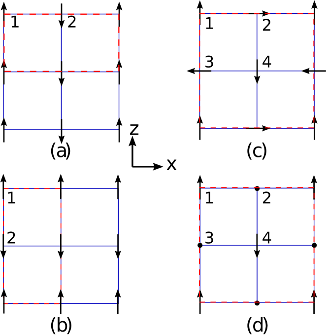
Figure 1: Magnetic ground state configurations for (a) $\mathbf{Q}_{1}=\left(\pi,0\right)$ stripe order (b) $\mathbf{Q}_{2}=\left(0,\pi\right)$ stripe order (c) double-Q non-collinear (orthomagnetic) order and (d) double-Q non-uniform magnetic order. The dashed rectangle denotes the magnetic unit cell in each case. While (a) and (b) are orthorhombic, (c) and (d) are tetragonal with a unit cell four times larger than in the paramagnetic phase.

Using an effective low-energy model for the orthomagnetic state, we also calculate its spin-wave spectrum. In contrast to the stripe state, which displays a doubly-degenerate Goldstone mode, we find three Goldstone modes that give rise to two distinct spin-wave branches emerging from both $\mathbf{Q}_{1}$ and $\mathbf{Q}_{2}$. Furthermore, the three diagonal components of the spin-spin correlation function $\mathcal{S}_{xx}$, $\mathcal{S}_{yy}$, $\mathcal{S}_{zz}$, and the off-diagonal $\mathcal{S}_{xz}$ term, display spin-wave modes at low energies, implying that in all directions the excitations behave as gapless transverse-like modes, as expected for a non-collinear configuration that breaks all spin-space rotational symmetries. We argue that these signatures of the low-energy spin spectrum of the orthomagnetic state can be unambiguously distinguished from those arising from domains of stripe magnetic states in both unpolarized and polarized neutron scattering measurements. Thus, our studies provide concrete criteria to establish the existence of the orthomagnetic state beyond the indirect evidence of an absent orthorhombic distortion.

Our paper is organized as follows: in Section II, we review the microscopic model for the magnetic instability proposed in Refs. rafael ; Eremin10 and extend the analysis by including the effects of the residual electronic interactions and by computing the Ginzburg-Landau coefficients in the regime far from perfect nesting. In Section III we present an effective low-energy model for the orthomagnetic state whose spin-wave dispersions can be appropriately treated within the Holstein-Primakoff formalism. We calculate both the spin-wave modes and the components of the spin-spin correlation function, contrasting to the stripe magnetic case. Section IV is devoted to the concluding remarks and to the applicability of our results to other materials that may display orthomagnetic order, such as the heavy-fermion related compound GdRhIn₅ granado .

II Microscopic mechanism for the orthomagnetic order

We start with the itinerant three-band model that was previously used to explain the magnetic properties of the iron arsenides near perfect nesting rafael ; Eremin10 . The non-interacting part consists of:

$$H_{0}=\sum_{\mathbf{k}a\alpha}\varepsilon_{a,\mathbf{k}}c_{a,\mathbf{k}\alpha}^{\dagger}c_{a,\mathbf{k}\alpha}$$ (1)

where $\alpha$ is the spin index, $\mathbf{k}$ is the momentum, and $a=h$, $e_{1}$, $e_{2}$ refer to, respectively, the central hole pocket and the electron pockets centered at $\mathbf{Q}_{1}=\left(\pi,0\right)$ and $\mathbf{Q}_{2}=\left(0,\pi\right)$. The band dispersions near the Fermi level can be conveniently parametrized as:

$$\varepsilon_{h,\mathbf{k}} =-\varepsilon_{\mathbf{k}}$$

$$\varepsilon_{e_{1},\mathbf{k}+\mathbf{Q}_{1}} =\varepsilon_{\mathbf{k}}-\left(\delta_{\mu}+\delta_{m}\cos 2\theta\right)$$

$$\varepsilon_{e_{2},\mathbf{k}+\mathbf{Q}_{2}} =\varepsilon_{\mathbf{k}}-\left(\delta_{\mu}-\delta_{m}\cos 2\theta\right)$$ (2)

where $\varepsilon_{\mathbf{k}}=\frac{k^{2}}{2m}-\varepsilon_{0}$ is a parabolic-like band dispersion, $\theta$ is the angle around the electron pocket, $\delta_{m}$ describes the ellipticity of the electron pockets, and $\delta_{\mu}$ is proportional to changes in the carrier concentration (doping). Note that for $\delta_{m}=\delta_{\mu}=0$, the system has perfect particle-hole symmetry and the hole and electron pockets are perfectly nested.

Following Ref. chubukov ; maiti , there are eight types of purely electronic interactions connecting the three Fermi pockets, corresponding to density-density ($U_{1}$, $U_{4}$, $U_{5}$, $U_{6}$), spin-exchange ($U_{2}$, $U_{7}$) and pair-hopping ($U_{3}$, $U_{8}$) interactions respectively. The interaction Hamiltonian is:

$$\begin{split}H_{\text{int}}&=U_{1}\sum c_{h\alpha}^{\dagger}c_{e_{i}\beta}^{\dagger}c_{e_{i}\beta}c_{h\alpha}+U_{2}\sum c_{h\alpha}^{\dagger}c_{e_{i}\beta}^{\dagger}c_{h\beta}c_{e_{i}\alpha}\\ &+\frac{U_{3}}{2}\sum(c_{h\alpha}^{\dagger}c_{h\beta}^{\dagger}c_{e_{i}\beta}c_{e_{i}\alpha}+\mathrm{h.c.})\\ &+\frac{U_{4}}{2}\sum c_{e_{i}\alpha}^{\dagger}c_{e_{i}\beta}^{\dagger}c_{e_{i}\beta}c_{e_{i}\alpha}+\frac{U_{5}}{2}\sum c_{h\alpha}^{\dagger}c_{h\beta}^{\dagger}c_{h\beta}c_{h\alpha}\\ &+U_{6}\sum c_{e_{1}\alpha}^{\dagger}c_{e_{2}\beta}^{\dagger}c_{e_{2}\beta}c_{e_{1}\alpha}+U_{7}\sum c_{e_{1}\alpha}^{\dagger}c_{e_{2}\beta}^{\dagger}c_{e_{1}\beta}c_{e_{2}\alpha}\\ &+\frac{U_{8}}{2}\sum(c_{e_{1}\alpha}^{\dagger}c_{e_{1}\beta}^{\dagger}c_{e_{2}\beta}c_{e_{2}\alpha}+\mathrm{h.c.})\end{split}$$ (3)

For simplicity of notation, the momentum indices are all suppressed with the implicit constraint of momentum conservation. To study the instability towards magnetic order, we project all the interactions in the spin-density wave (SDW) channel – which is the leading one according to RG and fRG calculations maiti ; Thomale09 . The only interactions that contribute directly to the SDW instability are $U_{1}$ and $U_{3}$. The partition function, restricted to this channel only, can then be written in the functional field form:

$$\mathcal{Z}=\int\mathcal{D}c^{\dagger}\mathcal{D}c\ \exp(-S)$$ (4)

with the action :

$$S=\int_{0}^{\beta}\mathrm{d}\tau\ \sum_{i\mathbf{k}\sigma}c_{i\mathbf{k}\sigma}^{\dagger}\partial_{\tau}c_{i\mathbf{k}\sigma}+H_{0}+H_{\mathrm{SDW}}$$ (5)

and the SDW-decoupled interaction:

$$H_{\text{SDW}}=-I\sum_{i\mathbf{k}\mathbf{k}^{\prime}\mathbf{q}}\left(c_{h\mathbf{k}\alpha}^{\dagger}\boldsymbol{\sigma}_{\alpha\beta}c_{e_{i}\mathbf{k}+\mathbf{q}\beta}\right)\cdot\left(c_{e_{i}\mathbf{k}^{\prime}\gamma}^{\dagger}\boldsymbol{\sigma}_{\gamma\delta}c_{h\mathbf{k}^{\prime}-\mathbf{q}\delta}\right)$$ (6)

where $I=U_{1}+U_{3}$. We now introduce the Hubbard-Stratonovich fields $\mathbf{M}_{i}$, whose mean value is proportional to the staggered magnetization with ordering vector $\mathbf{Q}_{i}$, i.e. $\left\langle\mathbf{M}_{i}\right\rangle=I\sum_{\mathbf{k}}\left\langle c_{h\mathbf{k}\alpha}^{\dagger}\boldsymbol{\sigma}_{\alpha\beta}c_{e_{i}\mathbf{k}+\mathbf{q}\beta}\right\rangle$, via $\exp\left(-H_{\text{SDW}}\right)\propto\int\mathcal{D}\mathbf{M}_{i}\exp\left(-S_{\mathrm{SDW}}\left[\mathbf{M}_{i}\right]\right)$ with:

$$S_{\mathrm{SDW}}\left[\mathbf{M}_{i}\right] =\sum_{i\mathbf{q}}\frac{\mathbf{M}_{i\mathbf{q}}\cdot\mathbf{M}_{i-\mathbf{q}}}{I}$$ (7)

$$-\sum_{i\mathbf{q}\mathbf{k}}\left(\mathbf{M}_{i\mathbf{q}}\cdot c_{e_{i}\mathbf{k}\gamma}^{\dagger}\boldsymbol{\sigma}_{\gamma\delta}c_{h\mathbf{k}-\mathbf{q}\delta}+\mathrm{h.c.}\right)$$

Following Ref. rafael , we then integrate out the electronic degrees of freedom, obtaining an effective action for the magnetic degrees of freedom:

$$\mathcal{Z} =\int\mathcal{D}c^{\dagger}\mathcal{D}c\,\mathcal{D}\mathbf{M}_{i}\ \exp\left(-S\left[c^{\dagger},\mathbf{M}_{i}\right]\right)$$

$$=\int\mathcal{D}\mathbf{M}_{i}\ \exp\left(-S_{\mathrm{eff}}\left[\mathbf{M}_{i}\right]\right)$$ (8)

For a finite-temperature magnetic transition, $S_{\mathrm{eff}}\left[\mathbf{M}_{i}\right]=F\left[\mathbf{M}_{i}\right]/T$, where $F\left[\mathbf{M}_{i}\right]$ is the free energy. Near the magnetic transition, we can expand the action in powers of the magnetic order parameters, deriving the Ginzburg-Landau expansion:

$$\begin{split}S_{\mathrm{eff}}&\left[\mathbf{M}_{i}\right]=\frac{a}{2}(\mathbf{M}_{1}^{2}+\mathbf{M}_{2}^{2})+\frac{u}{4}(\mathbf{M}_{1}^{2}+\mathbf{M}_{2}^{2})^{2}\\ &-\frac{g}{4}(\mathbf{M}_{1}^{2}-\mathbf{M}_{2}^{2})^{2}+w(\mathbf{M}_{1}\cdot\mathbf{M}_{2})^{2}\end{split}$$ (9)

In the vicinity of the magnetic transition, $a\approx N_{f}(T-T_{N})$, where $N_{f}$ is the density of states at the Fermi surface. The coefficients $u$, $g$, and $w$ are given by rafael :

$$u =A+B$$

$$g =B-A$$

$$w =0$$ (10)

with:

$$A =\int_{k}G_{h,\mathbf{k}}^{2}G_{e_{1},\mathbf{k}+\mathbf{Q}_{1}}^{2}$$

$$=\int_{k}\left(\frac{1}{i\omega_{n}+\varepsilon_{\mathbf{k}}}\right)^{2}\left(\frac{1}{i\omega_{n}-\varepsilon_{\mathbf{k}}+\delta_{\mu}+\delta_{m}\cos 2\theta}\right)^{2}\quad,$$

$$B =\int_{k}G_{h,\mathbf{k}}^{2}G_{e_{1},\mathbf{k+Q_{1}}}G_{e_{2},\mathbf{k}+\mathbf{Q}_{2}}$$

$$=\int_{k}\left(\frac{1}{i\omega_{n}+\varepsilon_{\mathbf{k}}}\right)^{2}\frac{1}{i\omega_{n}-\varepsilon_{\mathbf{k}}+\delta_{\mu}+\delta_{m}\cos 2\theta}$$

$$\ \times\frac{1}{i\omega_{n}-\varepsilon_{\mathbf{k}}+\delta_{\mu}-\delta_{m}\cos 2\theta}\quad,$$ (11)

Here, $G_{a,\mathbf{k}}$ is the non-interacting fermionic Green’s function for pocket $a$, $G_{a,\mathbf{k}}^{-1}=i\omega_{n}-\varepsilon_{a,\mathbf{k}}$, and $\int_{k}\rightarrow T\sum_{n}\int\frac{d\mathbf{k}}{\left(2\pi\right)^{d}}$, with Matsubara frequency $\omega_{n}=\left(2n+1\right)\pi T$. After integrating out the momentum, we obtain:

$$A =N_{f}T\pi\sum_{n=0}^{\infty}\mathrm{Im}\int_{\theta}\frac{1}{\left(i\omega_{n}+\frac{\delta_{\mu}}{2}+\frac{\delta_{m}}{2}\,\cos 2\theta\right)^{3}}$$

$$B =N_{f}T\pi\sum_{n=0}^{\infty}\mathrm{Im}\int_{\theta}\frac{i\omega_{n}+\frac{\delta_{\mu}}{2}}{\left(\left(i\omega_{n}+\frac{\delta_{\mu}}{2}\right)^{2}-\left(\frac{\delta_{m}}{2}\,\cos 2\theta\right)^{2}\right)^{2}}$$ (12)

with $\int_{\theta}=\int_{0}^{2\pi}\frac{d\theta}{2\pi}$. A straightforward minimization of Eq. (9) reveals that the stripe magnetic state is the global free energy minimum for $g>\max\left(0,-w\right)$, whereas a tetragonal magnetic state is the lowest energy ground state for $g<\max\left(0,-w\right)$. Since in the model above $w=0$, the sign of $g$ determines uniquely the symmetry of the magnetic ground state. Note that the free energy functional is bounded for $u>\max\left(g,0,-w\right)$.

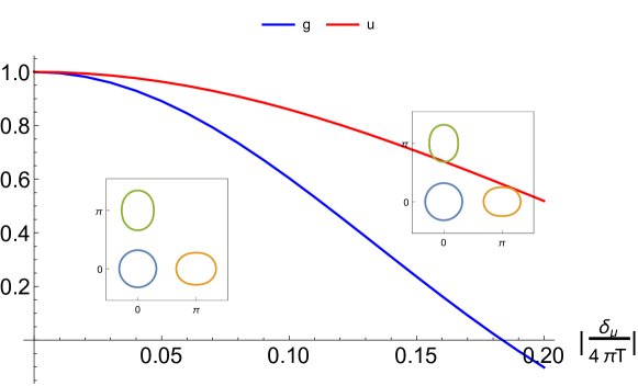
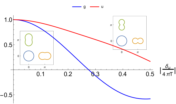
Figure 2: Quartic Ginzburg-Landau coefficients $u$ (red) and $g$ (blue) of the free energy (9) as function of $|\delta_{\mu}|/(4\pi T)$ for $\delta_{m}/(4\pi T)=0.2$ (top) and $\delta_{m}/(4\pi T)=0.5$ (bottom). The insets show the shape of the Fermi pockets for $\frac{\delta_{\mu}}{4\pi T}=-0.05\ \text{and}\ -0.2$ in the top panel, $\frac{\delta_{\mu}}{4\pi T}=-0.1\ \text{and}\ -0.4$ in the bottom panel. Note that $u$ and $g$ are normalized by their values at $\delta_{\mu}=0$. For $g>0$, the magnetic ground state is the stripe state, which lowers the tetragonal symmetry to orthorhombic. For $g<0$, tetragonal symmetry is preserved, and either a non-collinear or a non-uniform double-$\mathbf{Q}$ magnetic state arises. Notice that the free energy remains bounded as long as $u>0$.

The previous analysis of the Ginzburg-Landau coefficients (12) in Ref. rafael focused on the regime near perfect nesting, where $\delta_{\mu},\delta_{m}\ll T$. In this case, $g\propto\delta_{m}^{2}>0$ and the ground state is the stripe magnetic one. Here, we extend the analysis beyond small deviations from perfect nesting by numerically computing Eqs. (12) for arbitrary $\delta_{\mu}/T$, $\delta_{m}/T$ (the constraint $\delta_{m}\geq\delta_{\mu}$ is imposed to ensure that hot spots are present, as seen experimentally). To mimic the phase diagrams of $\text{Ba}(\text{Fe}_{1-x}\text{Mn}_{x})_{2}\text{As}_{2}$, $(\text{Ba}_{1-x}\text{K}_{x})\text{Fe}_{2}\text{As}_{2}$, and $(\text{Ba}_{1-x}\text{Na}_{x})\text{Fe}_{2}\text{As}_{2}$, we change the parameter $\delta_{\mu}$ (proportional to the carrier concentration) for a fixed value of the ellipticity $\delta_{m}$. Note that Eq. (12) implies that the behavior of $u$ and $g$ depend only on $|\delta_{\mu}|$. Fig 2 shows the results for $\delta_{m}/T=0.8\pi$ and $\delta_{m}/T=2\pi$. For small values of $|\delta_{\mu}|$, both $u$ and $g$ are positive, and the stripe magnetic state is favored. However, as $|\delta_{\mu}|$ becomes larger, regardless of the value of $\delta_{m}$, $g$ becomes negative, indicating that the magnetic ground state becomes a double-$\mathbf{Q}$ tetragonal phase. The evolution of the Fermi surfaces as $|\delta_{\mu}|$ increases, for the case of hole-doping, is shown in the insets. Since $u$ remains positive when $g$ first changes sign, the free energy remains bounded, i.e. the mean-field transition is second-order. These results are in qualitative agreement with the phase diagrams of $\text{Ba}(\text{Fe}_{1-x}\text{Mn}_{x})_{2}\text{As}_{2}$, $(\text{Ba}_{1-x}\text{K}_{x})\text{Fe}_{2}\text{As}_{2}$, and $(\text{Ba}_{1-x}\text{Na}_{x})\text{Fe}_{2}\text{As}_{2}$, which display the tetragonal magnetic phase only for sufficiently strong doping concentration. We note that a tetragonal magnetic state was also reported in other itinerant approaches for the iron pnictides Eremin10 ; Lorenzana08 ; Brydon11 , as well as in a strong-coupling two-orbital ladder model Berg10 .

Figure 3: Top panel: The vertex that couples the magnetic order parameter to the low-energy fermionic states, which has a $\mathbf{M}_{i}\cdot\boldsymbol{\sigma}$ structure. Solid lines refer to the non-interacting electronic Green’s functions. Bottom panel: the Feynman diagrams containing the leading-order corrections to the free energy arising from the residual $U_{7}$ interaction.

Because $w=0$ in our model, when $g$ becomes negative the system does not distinguish between the two possible tetragonal magnetic states, namely, the orthomagnetic one ($w>0$, $\mathbf{M}_{1}\perp\mathbf{M}_{2}$) and the non-uniform one ($w<0$, $\mathbf{M}_{1}\parallel\mathbf{M}_{2}$). Although the terms arising purely from the band structure do not contribute to the $w$ coefficient, the residual interactions in Eq. (3) that do not participate in the SDW instability (namely $U_{2}$, $U_{4}$, $U_{5}$, $U_{6}$, $U_{7}$, and $U_{8}$) give rise to such a term, as pointed out in Ref. Eremin10 . Computing the contributions of the residual interactions to the action, we obtain:

$$\tilde{S}\left[\mathbf{M}_{i}\right] =\frac{1}{4}\left(-\tilde{u}_{2}+\tilde{u}_{4}+\tilde{u}_{5}+\tilde{u}_{6}-\tilde{u}_{7}+\tilde{u}_{8}\right)\left(\mathbf{M}_{1}^{2}+\mathbf{M}_{2}^{2}\right)^{2}$$

$$-\frac{1}{4}\left(-\tilde{g}_{4}+\tilde{g}_{6}-\tilde{g}_{7}+\tilde{g}_{8}\right)\left(\mathbf{M}_{1}^{2}-\mathbf{M}_{2}^{2}\right)^{2}$$

$$+\tilde{w}_{7}\left(\mathbf{M}_{1}\cdot\mathbf{M}_{2}\right)^{2}$$ (13)

The Ginzburg-Landau coefficients can be obtained in a straightforward way using diagrammatics. In Fig. 3 we show the two diagrams arising from the $U_{7}$ interaction, which contribute to $\tilde{u}_{7}$, $\tilde{g}_{7}$, and $\tilde{w}_{7}$. Additional computational details are discussed in Appendix A. The coefficients of the quartic symmetric term are given by:

$$\tilde{u}_{2} =8U_{2}\left(\int_{k}G_{h,\mathbf{k}}G_{e_{1},\mathbf{k}+\mathbf{Q}_{1}}^{2}\right)\left(\int_{k}G_{h,\mathbf{k}}^{2}G_{e_{1},\mathbf{k}+\mathbf{Q}_{1}}\right)$$

$$\tilde{u}_{4} =2U_{4}\left(\int_{k}G_{h,\mathbf{k}}G_{e_{1},\mathbf{k}+\mathbf{Q}_{1}}^{2}\right)^{2}$$

$$\tilde{u}_{5} =4U_{5}\left(\int_{k}G_{h,\mathbf{k}}^{2}G_{e_{1},\mathbf{k}+\mathbf{Q}_{1}}\right)^{2}$$

$$\tilde{u}_{6} =2U_{6}\left[2\left(\int_{k}G_{h,\mathbf{k}}G_{e_{1},\mathbf{k}+\mathbf{Q}_{1}}^{2}\right)^{2}\right.$$

$$\left.-\left(\int_{k}G_{h,\mathbf{k}}G_{e_{1},\mathbf{k}+\mathbf{Q}_{1}}G_{e_{2},\mathbf{k}+\mathbf{Q}_{2}}\right)^{2}\right]$$

$$\tilde{u}_{7} =2U_{7}\left(\int_{k}G_{h,\mathbf{k}}G_{e_{1},\mathbf{k}+\mathbf{Q}_{1}}^{2}\right)^{2}$$

$$\tilde{u}_{8} =2U_{8}\left(\int_{k}G_{h,\mathbf{k}}G_{e_{1},\mathbf{k}+\mathbf{Q}_{1}}G_{e_{2},\mathbf{k}+\mathbf{Q}_{2}}\right)^{2}$$ (14)

whereas the coefficients of the quartic anti-symmetric term read:

$$\tilde{g}_{4} =2U_{4}\left(\int_{k}G_{h,\mathbf{k}}G_{e_{1},\mathbf{k}+\mathbf{Q}_{1}}^{2}\right)^{2}$$

$$\tilde{g}_{6} =2U_{6}\left[2\left(\int_{k}G_{h,\mathbf{k}}G_{e_{1},\mathbf{k}+\mathbf{Q}_{1}}^{2}\right)^{2}\right.$$

$$\left.-\left(\int_{k}G_{h,\mathbf{k}}G_{e_{1},\mathbf{k}+\mathbf{Q}_{1}}G_{e_{2},\mathbf{k}+\mathbf{Q}_{2}}\right)^{2}\right]$$

$$\tilde{g}_{7} =2U_{7}\left(\int_{k}G_{h,\mathbf{k}}G_{e_{1},\mathbf{k}+\mathbf{Q}_{1}}^{2}\right)^{2}$$

$$\tilde{g}_{8} =2U_{8}\left(\int_{k}G_{h,\mathbf{k}}G_{e_{1},\mathbf{k}+\mathbf{Q}_{1}}G_{e_{2},\mathbf{k}+\mathbf{Q}_{2}}\right)^{2}$$ (15)

and the coefficient of the quartic scalar-product term yields:

$$\tilde{w}_{7}=4U_{7}\left(\int_{k}G_{h,\mathbf{k}}G_{e_{1},\mathbf{k}+\mathbf{Q}_{1}}G_{e_{2},\mathbf{k}+\mathbf{Q}_{2}}\right)^{2}$$ (16)

At perfect nesting, an overall factor proportional to the Green’s functions product $\left(\int_{k}G_{h,\mathbf{k}}^{2}G_{e_{1},\mathbf{k}+\mathbf{Q}_{1}}\right)^{2}$ appears in all terms. In this limit, our results become identical to those found in Ref. Eremin10 , which computed the corrections to the magnetic ground state energy in the ordered state using a sequence of Bogoliubov transformations. In the paramagnetic state, however, which is our case of interest, this Green’s functions product vanishes – as also pointed out in Ref. Eremin10 . The corrections due to the residual interactions naturally become non-zero – and in fact positive – once one considers small deviations from perfect nesting. For $\tilde{w}_{7}$, we find:

$$\tilde{w}_{7}\approx 4U_{7}\left(\frac{7\zeta(3)N_{f}\delta_{\mu}}{8\pi^{2}T^{2}}\right)^{2}$$ (17)

Because the band dispersions do not contribute to the term $\left(\mathbf{M}_{1}\cdot\mathbf{M}_{2}\right)^{2}$, the fact that $\tilde{w}_{7}>0$ is very important, as it implies that the residual interaction $U_{7}$ selects the orthomagnetic state over the non-uniform state (assuming that $U_{7}>0$, as one would expect). Therefore, when $g_{\mathrm{eff}}=g+\tilde{g}$ changes sign, the system tends to form the non-collinear tetragonal magnetic state shown in Fig. 1c. Dimensional analysis of the relevant Feynman diagrams reveals that $\tilde{g}/g\propto U_{i}N_{f}$, where $U_{i}$ is the appropriate combination of residual interactions. Therefore, in our weak-coupling approach, because $U_{i}N_{f}\ll 1$, it follows that $\tilde{g}\ll g$ – unless $g$ itself is close to zero. As a result, although the contribution from $\tilde{g}$ may change slightly the value of $\delta_{\mu}$ for which $g_{\mathrm{eff}}=g+\tilde{g}$ vanishes, it cannot preclude the sign-changing found in Fig. 2 from taking place. The case of $w_{\mathrm{eff}}=w+\tilde{w}$ is fundamentally different, since $w=0$, making $\tilde{w}$ the leading non-vanishing term.

In the next section, we will discuss the magnetic spectrum of such a state. Before proceeding, we emphasize that, as pointed out by two of us in a previous communication xiaoyu , other mechanisms may favor a different sign for the $w$ coefficient – such as the coupling to soft Neel-like magnetic fluctuations – which could stabilize the non-uniform tetragonal magnetic state shown in Fig. 1d. We also note that the Ginzburg-Landau expansion (9) is very general for two SDW order parameters that preserve spin-rotational and tetragonal symmetries. To obtain its coefficients, besides the Hertz-Millis approach employed here, one can also fit the free energy directly to first-principle band structures. This was done in Ref. giovannetti , which also found the orthomagnetic state to be a ground state for certain parameter ranges.

III Spin-wave spectrum

Having established the conditions under which the orthomagnetic state becomes the ground state of the system, we now discuss its experimental manifestations. The most evident one is the lack of tetragonal symmetry breaking, since the orthomagnetic order has an equal weight of the order parameters $\mathbf{M}_{1}$ and $\mathbf{M}_{2}$ associated with the ordering vectors $\mathbf{Q}_{1}=\left(\pi,0\right)$ and $\mathbf{Q}_{2}=\left(0,\pi\right)$, respectively. The preservation of $C_{4}$ symmetry can in principle be detected by x-ray or neutron scattering via the absence of splitting of the lattice Bragg peaks across the magnetic transition. However, given the resolution limitations of scattering measurements, it is desirable to consider other properties that identify unambiguously the orthomagnetic state.

In this section, we study in details the spin-wave spectrum of the orthomagnetic phase, comparing it to the stripe phase. As we are interested in the low-energy behavior, there are two alternative approaches to compute the spin-wave spectrum: the first is by evaluating self-consistently the poles of the spin-spin correlation function deep inside the magnetically ordered state within the itinerant approach described in the previous section spin_waves_itinerant_MSDW ; knolle01 ; knolle02 . The second alternative is to build a phenomenological localized-spin model that gives the same ground states as the itinerant model, and then use Holstein-Primakoff (HP) bosons to compute the spin-wave dispersionzhao ; harriger . Given the simplicity of the latter, we here consider a Heisenberg model on a two-dimensional square lattice, with nearest-neighbor and next-nearest neighbor interactions:

$$H=J_{1}\sum_{\langle i,j\rangle}\mathbf{S}_{i}\cdot\mathbf{S}_{j}+J_{2}\sum_{\langle\langle i,j\rangle\rangle}\mathbf{S}_{i}\cdot\mathbf{\mathbf{S}}_{j}-\frac{K}{S^{2}}\sum_{\langle i,j\rangle}(\mathbf{S}_{i}\cdot\mathbf{S}_{j})^{2}$$ (18)

where $\langle...\rangle$ and $\langle\langle...\rangle\rangle$ denote nearest-neighbors and next-nearest neighbors, and $J_{1}>0$, $J_{2}>J_{1}/2$ are the respective antiferromagnetic exchange interactions. The biquadratic term $K$ selects between the stripe phase ($K>0$) and the orthomagnetic phase ($K<0$) in the classical regime. We emphasize that this is a phenomenological model constructed to describe the ground states obtained in Section II. Indeed, if it was the classical $J_{1}$-$J_{2}$ model, $K$ would be restricted to small positive values only chandra . Instead, here $K$ should be understood as a phenomenological parameter, analogous to the parameter $g$ calculated in Eq. (9). In fact, a Ginzburg-Landau expansion of this toy Heisenberg model would result in a free energy equivalent to that of Eq. (9), evidencing the fact that both models share the same low-energy properties Batista11 . Therefore, the use of this localized-spin model should be understood simply as a tool to evaluate the spin-wave spectrum, and not an implication that local moments are necessarily present in the system. Incidentally, we note that other Heisenberg models with ring exchange interactions can also display orthomagnetic order Chubukov92 .

We emphasize that a strict two-dimensional model does not have long-range Heisenberg magnetic order, according to Mermin-Wagner theorem. As a result, we assume here that the system is formed by weakly-coupled layers. Such a small inter-layer coupling can nevertheless be neglected in what regards the main properties of the spin-wave dispersions. To obtain the spin-wave spectrum of the Hamiltonian (18), we follow Refs. Carlson04 ; haraldsen and introduce locally Holstein-Primakoff (HP) bosons for each of the $r$ spins in a single magnetic unit cell:

$$\mathbf{S}_{z}^{(r)} =S-a^{(r)\dagger}a^{(r)}$$

$$\mathbf{S}_{+}^{(r)} =\sqrt{2S-a^{(r)\dagger}a^{(r)}}\ a^{(r)}$$ (19)

$$\mathbf{S}_{-}^{(r)} =a^{(r)\dagger}\sqrt{2S-a^{(r)\dagger}a^{(r)}}$$

Note that the spin coordinate system is defined locally, such that the local spin is always parallel to the local $+\hat{\mathbf{z}}$ axis. For convenience, the two-dimensional lattice plane $xy$ is chosen to be the $xz$ spin-plane, as shown in Fig. 1. Since different types of spins within a magnetic unit cell have their own degree of freedom, the number of HP bosons (labeled by $r$) is equal to the number of spins within a magnetic unit cell. Thus, the stripe state has $r=1,2$ whereas the orthomagnetic state has $r=1,2,3,4$, as labeled in Fig. 1. The Fourier transform of the HP bosons is defined as

$$a_{\mathbf{k}}^{(r)}=\sum_{i\in r}a_{i}^{(r)}e^{-i\mathbf{k}\cdot\mathbf{x}_{i}^{(r)}}$$ (20)

where $i$ labels different magnetic unit cells, and $\mathbf{x}_{i}^{(r)}$ is the position of the $r$-th spin in the $i$-th magnetic unit cell. For convenience, we define:

$$\Psi_{\mathbf{k}}^{\dagger}\equiv\left(a_{\mathbf{k}}^{(1)\dagger},a_{-\mathbf{k}}^{(1)},a_{\mathbf{k}}^{(2)\dagger},a_{-\mathbf{k}}^{(2)},...\right)$$ (21)

Because we are interested in the classical limit, we perform a large $S$ expansion and keep only terms that are quadratic in the bosonic operators. In this case, the Heisenberg Hamiltonian can be re-expressed as:

$$H=H_{0}+\frac{1}{2}\sum_{\mathbf{k}}\Psi_{\mathbf{k}}^{\dagger}\hat{\mathcal{H}}_{\mathbf{k}}\Psi_{\mathbf{k}}$$ (22)

where $H_{0}$ is the classical ground state energy for a given spin configuration. The spin-wave modes can be obtained by a generalized Bogoliubov transformation, $\Psi_{\mathbf{k}}=\hat{\mathcal{U}}_{\mathbf{k}}\Phi_{\mathbf{k}}$. To ensure that the transformed operators satisfy the correct bosonic commutation relations, it is convenient to introduce the Bogoliubov metric:

$$\hat{\eta}=\text{diag}(1,-1,1,-1,...)$$ (23)

Then, the generalized Bogoliubov transformation satisfies:

$$\hat{\mathcal{U}}_{\mathbf{k}}^{\dagger}\,\hat{\eta}\,\hat{\mathcal{U}}_{\mathbf{k}} =\mathbb{\hat{\eta}}$$

$$\hat{\mathcal{U}}_{\mathbf{k}}^{-1}\left(\hat{\eta}\,\hat{\mathcal{H}}_{\mathbf{k}}\right)\hat{\mathcal{U}}_{\mathbf{k}} =\left(\mathcal{\hat{\eta}\,\hat{\mathcal{H}}_{\mathbf{k}}}\right)^{\text{diag}}$$ (24)

The spin-wave modes are therefore the eigenvalues of $\hat{\eta}\,\hat{\mathcal{H}}_{\mathbf{k}}$.

III.1 Stripe phase: spin-wave modes

As discussed above, the stripe phase is the ground state of the model (18) for $K>0$. The spin-wave dispersion of the stripe phase was obtained previously in Refs. Carlson08 ; Applegate10 ; fang and here we rederive the results to compare them later with the orthomagnetic case. For concreteness, we first consider the stripe phase with ordering vector $\mathbf{Q}_{1}=\left(\pi,0\right)$. As shown in Fig.1(a), there are two spins per magnetic unit cell, whose HP operators we denote by $a_{\mathbf{k}}^{(1)}$ and $a_{\mathbf{k}}^{(2)}$. Note that, with respect to the spin coordinate system defined on site 1, the spin on site 2 is rotated by $180^{\circ}$, yielding:

$$\mathbf{S}^{(2)}=\left(-S_{x}^{(2)},S_{y}^{(2)},-S_{z}^{(2)}\right)_{(1)}$$ (25)

Using the Holstein-Primakoff transformation defined in Eq. 21, we find that the large-$S$ Hamiltonian is given by:

$$\hat{\mathcal{H}}_{\mathbf{k}}=\left(\begin{array}[]{cccc}\epsilon_{\mathbf{k}}&0&0&\Delta_{\mathbf{k}}\\ 0&\epsilon_{\mathbf{k}}&\Delta_{\mathbf{k}}&0\\ 0&\Delta_{\mathbf{k}}&\epsilon_{\mathbf{k}}&0\\ \Delta_{\mathbf{k}}&0&0&\epsilon_{\mathbf{k}}\end{array}\right)$$ (26)

with:

$$\epsilon_{\mathbf{k}} =2S\left[\left(J_{1}-2K\right)\cos k_{y}+2J_{2}+4K\right]$$

$$\Delta_{\mathbf{k}} =-2S\left(J_{1}+2K+2J_{2}\cos k_{y}\right)\cos k_{x}$$ (27)

The Hamiltonian is diagonalized via the Bogoliubov transformation

$$\hat{\mathcal{U}}_{\mathbf{k}}=\left(\begin{array}[]{cccc}u_{\mathbf{k}}&0&0&v_{\mathbf{k}}\\ 0&u_{\mathbf{k}}&v_{\mathbf{k}}&0\\ 0&v_{\mathbf{k}}&u_{\mathbf{k}}&0\\ v_{\mathbf{k}}&0&0&u_{\mathbf{k}}\end{array}\right)$$ (28)

with:

$$u_{\mathbf{k}}^{2}=\frac{1}{2}\left(1+\frac{\epsilon_{\mathbf{k}}}{\omega_{\mathbf{k}}}\right);\ v_{\mathbf{k}}^{2}=\frac{1}{2}\left(-1+\frac{\epsilon_{\mathbf{k}}}{\omega_{\mathbf{k}}}\right);\ u_{\mathbf{k}}v_{\mathbf{k}}=-\frac{1}{2}\frac{\Delta_{\mathbf{k}}}{\omega_{\mathbf{k}}}$$ (29)

yielding the doubly-degenerate eigenmode (i.e. spin-wave mode) of the bosonic system:

$$\omega_{\mathbf{k}}=\sqrt{\epsilon_{\mathbf{k}}^{2}-\Delta_{\mathbf{k}}^{2}}$$ (30)

The fact that there are two degenerate spin-wave modes for the stripe state is a consequence of the fact that $\omega_{\mathbf{k}+\mathbf{Q}_{1}}=\omega_{\mathbf{k}}$ and also of the collinear configuration of the spins. The spin-wave dispersion of the stripe phase with ordering vector $\mathbf{Q}_{2}=\left(0,\pi\right)$ can be calculated in the same way, yielding $\omega_{\mathbf{Q}_{2}}\left(k_{x},k_{y}\right)=\omega_{\mathbf{Q}_{1}}\left(k_{y},-k_{x}\right)$, as expected. In Fig. 4, we show the dispersion of the spin waves (30) for the two types of stripe orders in their respective magnetic Brillouin zones. The results obtained here are in agreement with those obtained previously elsewhere fang .

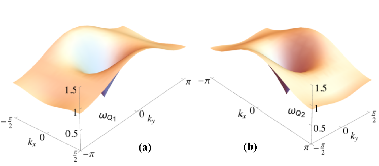
Figure 4: Spin-wave dispersions for the stripe phase with ordering vector $\mathbf{Q}_{1}=\left(\pi,0\right)$ (a) and $\mathbf{Q}_{2}=\left(0,\pi\right)$ (b). Both are doubly degenerate modes. The energies are in units of $4J_{2}S$ and the parameters used are $J_{1}=0.8J_{2}$ and $K=0.1J_{2}$.

III.2 Orthomagnetic phase: spin-wave modes

The orthomagnetic phase becomes the ground state of Eq. (18) for $K<0$. As shown in Fig.1(c), there are four spins per magnetic unit cell, giving rise to the HP operators $a_{\mathbf{k}}^{(1)}$, $a_{\mathbf{k}}^{(2)}$, $a_{\mathbf{k}}^{(3)}$, and $a_{\mathbf{k}}^{(4)}$. Because the spins on sites 2, 3, 4 correspond respectively to rotations of $90^{\circ}$, $180^{\circ}$, and $270^{\circ}$ relative to the spin on site 1, we define the local spin coordinate systems:

$$\mathbf{S}^{(2)} =(S_{z}^{(2)},S_{y}^{(2)},-S_{x}^{(2)})_{(1)}$$

$$\mathbf{S}^{(3)} =(-S_{z}^{(3)},S_{y}^{(3)},S_{x}^{(3)})_{(1)}$$

$$\mathbf{S}^{(4)} =(-S_{x}^{(4)},S_{y}^{(4)},-S_{z}^{(4)})_{(1)}$$ (31)

Introducing $\Psi_{\mathbf{k}}^{\dagger}$ as defined in Eq. (21) and substituting in the Hamiltonian, we obtain in the large-$S$ limit:

$$\hat{\mathcal{H}}_{\mathbf{k}}=\left(\begin{array}[]{cccc}\hat{A}_{\mathbf{k}}&\hat{B}_{\mathbf{k}}&\hat{C}_{\mathbf{k}}&\hat{D}_{\mathbf{k}}\\ \hat{B}_{\mathbf{k}}&\hat{A}_{\mathbf{k}}&\hat{D}_{\mathbf{k}}&\hat{C}_{\mathbf{k}}\\ \hat{C}_{\mathbf{k}}&\hat{D}_{\mathbf{k}}&\hat{A}_{\mathbf{k}}&\hat{B}_{\mathbf{k}}\\ \hat{D}_{\mathbf{k}}&\hat{C}_{\mathbf{k}}&\hat{B}_{\mathbf{k}}&\hat{A}_{\mathbf{k}}\end{array}\right)$$ (32)

where we defined four $2\times 2$ matrices, $\hat{A}_{\mathbf{k}}$, $\hat{B}_{\mathbf{k}}$, $\hat{C}_{\mathbf{k}}$, and $\hat{D}_{\mathbf{k}}$ of the form:

$$\hat{O}_{\mathbf{k}}=\left(\begin{array}[]{cc}O_{1,\mathbf{k}}&O_{2,\mathbf{k}}\\ O_{2,\mathbf{k}}&O_{1,\mathbf{k}}\end{array}\right)$$ (33)

with the matrix elements:

$$A_{1,\mathbf{k}} =4S\left(J_{2}-K\right),\ A_{2,\mathbf{k}}=-4SK$$

$$B_{1,\mathbf{k}} =S\left(J_{1}+2K\right)\cos k_{x},\ B_{2,\mathbf{k}}=-S\left(J_{1}-2K\right)\cos k_{x}$$

$$C_{1,\mathbf{k}} =S\left(J_{1}+2K\right)\cos k_{y},\ C_{2,\mathbf{k}}=-S\left(J_{1}-2K\right)\cos k_{y}$$

$$D_{1,\mathbf{k}} =0,\ D_{2,\mathbf{k}}=-4SJ_{2}\cos k_{x}\cos k_{y}$$ (34)

The generalized Bogoliubov transformation is given by:

$$\hat{\mathcal{U}}_{\mathbf{k}}=\left(\begin{array}[]{cccc}\hat{X}_{\mathbf{k}}&\hat{Y}_{\mathbf{k}}&\hat{Z}_{\mathbf{k}}&\hat{W}_{\mathbf{k}}\\ \hat{X}_{\mathbf{k}}&-\hat{Y}_{\mathbf{k}}&\hat{Z}_{\mathbf{k}}&-\hat{W}_{\mathbf{k}}\\ \hat{X}_{\mathbf{k}}&\hat{Y}_{\mathbf{k}}&-\hat{Z}_{\mathbf{k}}&-\hat{W}_{\mathbf{k}}\\ \hat{X}_{\mathbf{k}}&-\hat{Y}_{\mathbf{k}}&-\hat{Z}_{\mathbf{k}}&\hat{W}_{\mathbf{k}}\end{array}\right)$$ (35)

where the four $2\times 2$ matrices, $\hat{X}_{\mathbf{k}}$, $\hat{Y}_{\mathbf{k}}$, $\hat{Z}_{\mathbf{k}}$, and $\hat{W}_{\mathbf{k}}$ are also of the form (33). For $\hat{X}_{\mathbf{k}}$, the matrix elements are given by:

$$X_{1,\mathbf{k}}^{2} =\frac{1}{8}\left(1+\frac{\epsilon_{\mathbf{k}}}{\omega_{\mathbf{k}}}\right)$$

$$X_{2,\mathbf{k}}^{2} =\frac{1}{8}\left(-1+\frac{\epsilon_{\mathbf{k}}}{\omega_{\mathbf{k}}}\right)$$

$$X_{1,\mathbf{k}}X_{2,\mathbf{k}} =-\frac{1}{8}\frac{\Delta_{\mathbf{k}}}{\omega_{\mathbf{k}}}$$ (36)

with:

$$\epsilon_{\mathbf{k}} =A_{1,\mathbf{k}}+B_{1,\mathbf{k}}+C_{1,\mathbf{k}}+D_{1,\mathbf{k}}$$

$$\Delta_{\mathbf{k}} =A_{2,\mathbf{k}}+B_{2,\mathbf{k}}+C_{2,\mathbf{k}}+D_{2,\mathbf{k}}$$ (37)

and the spin-wave dispersions:

$$\omega_{\mathbf{k}}=\sqrt{\epsilon_{\mathbf{k}}^{2}-\Delta_{\mathbf{k}}^{2}}$$ (38)

For the other matrix elements, we find:

$$Y_{i,\mathbf{k}} =X_{i,\mathbf{k}+\mathbf{Q}_{1}}$$

$$Z_{i,\mathbf{k}} =X_{i,\mathbf{k}+\mathbf{Q}_{2}}$$

$$W_{i,\mathbf{k}} =X_{i,\mathbf{k}+\mathbf{Q}_{1}+\mathbf{Q}_{2}}$$ (39)

Therefore, there are four non-degenerate spin-wave dispersions of the bosonic system:

$$\omega_{1\mathbf{k}}=\omega_{\mathbf{k}};\ \omega_{2\mathbf{k}}=\omega_{\mathbf{k}+\mathbf{Q}_{1}};\ \omega_{3\mathbf{k}}=\omega_{\mathbf{k}+\mathbf{Q}_{2}};\ \omega_{4\mathbf{k}}=\omega_{\mathbf{k}+\mathbf{Q}_{1}+\mathbf{Q}_{2}}$$ (40)

with $\omega_{\mathbf{k}}$ given in Eq. (38). These four spin-wave dispersions are shifted with respect to each other by the ordering vectors of the orthomagnetic phase, corresponding to in-phase or out-of-phase combinations of the four HP bosons. All of them are shown in Fig. 5 in the magnetic unit cell of the orthomagnetic phase. We note that while $\omega_{1}$, $\omega_{2}$, and $\omega_{3}$ display gapless modes, corresponding to three Goldstone modes, the $\omega_{4}$ spin-wave dispersion is gapped. The fact that there are three Goldstone modes is a consequence of the non-collinear magnetic configuration of the orthomagnetic phase, which breaks completely all the spin-rotational symmetries of the system.

Figure 5: The spin-wave dispersions of the non-collinear orthomagnetic order in the magnetic Brillouin zone. The four dispersions are linked by a shift of the momentum coordinate system by the orthomagnetic ordering vectors. Here, the energies are in units of $4J_{2}S$ and the parameters are $J_{1}=0.8J_{2}$ and $K=-0.1J_{2}$.

III.3 Dynamic structure factors of the stripe and orthomagnetic phases

Having established the nature of the spin-wave modes in the stripe and orthomagnetic phases, we now proceed to compute the spin-spin correlation function $\mathcal{S}_{\mu\nu}$ in the non-magnetic unit cell, which can be measured by neutron scattering. We have haraldsen ; Carlson04 :

$$\mathcal{S}_{\mu\nu}\left(\mathbf{k},\omega\right)=\int_{-\infty}^{\infty}\frac{\mathrm{d}t}{2\pi}\ \mathrm{e}^{-i\omega t}\langle S_{\mathbf{k}}^{\mu}(0)S_{-\mathbf{k}}^{\nu}(t)\rangle$$ (41)

where $\mu\nu=x,y,z$ refer to the spin components and $\mathbf{S}_{\mathbf{k}}\equiv\sum_{r}\mathbf{S}_{r,\mathbf{k}}$ is the sum over all the $r$ spins in the magnetic unit cell. Here, the spin coordinate system is defined globally with respect to the neutron polarization, in contrast to the local coordinate system introduced in the previous subsection. For concreteness, hereafter we assume the incoming neutron to be polarized parallel to the spin on site $1$, i.e. parallel to the $\hat{\mathbf{z}}$ axis. Computation of Eq. (41) is straightforward with the aid of the HP bosons and the Bogoliubov transformation defined in the previous subsection. Denoting by $\tilde{a}_{\mathbf{k}}^{(r)}$ the Bogoliubov-transformed bosonic operators, the only non-zero terms, at $T=0$, are those of the form:

$$\int_{-\infty}^{\infty}\frac{\mathrm{d}t}{2\pi}\ \mathrm{e}^{-i\omega t}\left\langle\tilde{a}_{\mathbf{k}}^{(r)}\left(0\right)\tilde{a}_{\mathbf{k}}^{\dagger(r)}\left(t\right)\right\rangle=\delta\left(\omega-\omega_{r,\mathbf{k}}\right)$$ (42)

We first consider the stripe phase with the two possible ordering vectors $\mathbf{Q}_{1}=\left(\pi,0\right)$ and $\mathbf{Q}_{2}=\left(0,\pi\right)$. We find that only the transverse components $\mathcal{S}_{xx}=\mathcal{S}_{yy}$ are non-zero, i.e. the longitudinal component $S_{zz}$ and the off-diagonal components $\mathcal{S}_{i\neq j}$ do not acquire spin-wave contributions. We obtain:

$$\mathcal{S}_{xx}^{\mathbf{Q}_{i}}\left(\mathbf{k},\omega\right)=2S\left(u_{\mathbf{k}}-v_{\mathbf{k}}\right)^{2}\delta\left(\omega-\omega_{\mathbf{k}}^{\mathbf{Q}_{i}}\right)$$ (43)

where $u_{\mathbf{k}},v_{\mathbf{k}}$ are given by Eq. (29) and $\omega_{\left(k_{x},k_{y}\right)}^{\mathbf{Q}_{2}}=\omega_{\left(-k_{y},k_{x}\right)}^{\mathbf{Q}_{1}}$, with $\omega_{\mathbf{k}}^{\mathbf{Q}_{1}}$ given by Eq. (30). The total spin-spin correlation function, $\mathcal{S}=\sum_{i}\mathcal{S}_{ii}$ is then simply $\mathcal{S}\left(\mathbf{k},\omega\right)=2\mathcal{S}_{xx}\left(\mathbf{k},\omega\right)$. In Fig. 6, we plot $\mathcal{S}(\mathbf{k},\omega)$ for both the $\mathbf{Q}_{1}$ and $\mathbf{Q}_{2}$ stripe phases separately, as well as for a system containing equal domains of $\mathbf{Q}_{1}$ and $\mathbf{Q}_{2}$:

$$\mathcal{S}_{\mathrm{domain}}\left(\mathbf{k},\omega\right)=\frac{1}{2}\mathcal{S}^{\mathbf{Q}_{1}}\left(\mathbf{k},\omega\right)+\frac{1}{2}\mathcal{S}^{\mathbf{Q}_{2}}\left(\mathbf{k},\omega\right)$$ (44)

The latter is the case relevant for the real systems, since twin domains are always formed in the iron pnictides. In all the plots, the delta function is replaced by a Lorentzian with width $\gamma=0.05$ in units of $2J_{2}S$. From the figure, we see that the system with twin domains display anisotropic spin-wave branches emerging from the ordering vectors $\mathbf{Q}_{1}=\left(\pi,0\right)$ and $\mathbf{Q}_{2}=\left(0,\pi\right)$, as expected. In all cases, the structure factor vanishes at center of the Brillouin zone, but diverges at the ordering vectors $\mathbf{Q}_{i}$. Therefore, expanding the spin-wave dispersion around the ordering vector $\mathbf{Q}_{i}$ yields ($\theta$ denote the polar angle between $\mathbf{k}$ and $\hat{\mathbf{k}}_{x}$):

$$\omega_{\mathbf{k}+\mathbf{Q}_{i}}\approx 4S\left|\mathbf{k}\right|\sqrt{\left(J_{2}+K+\frac{J_{1}}{2}\right)\left(J_{2}+K\pm\frac{J_{1}}{2}\cos 2\theta\right)}$$ (45)

which is anisotropic along the $k_{x}$ and $k_{y}$ axis, as expected. In the previous expression, the upper (lower) sign refers to $\mathbf{Q}_{1}$ ($\mathbf{Q}_{2}$).

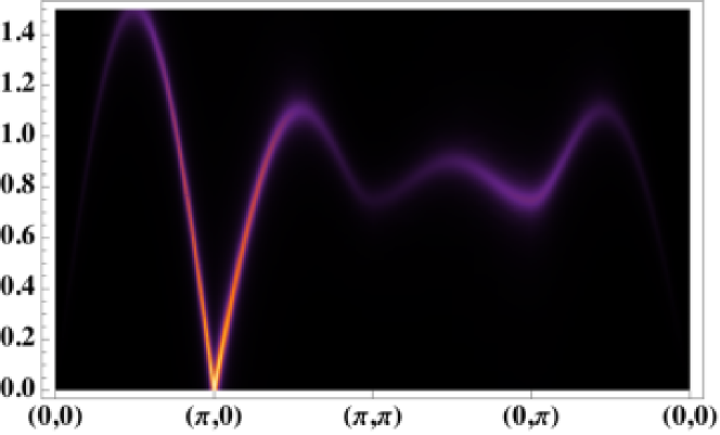
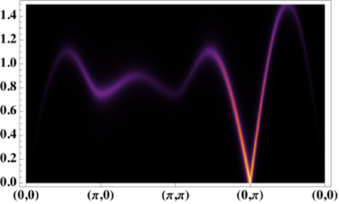
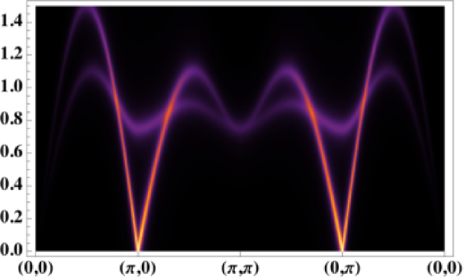
Figure 6: The total spin-spin structure factor $\mathcal{S}=\sum_{i}\mathcal{S}_{ii}=2S_{xx}$ for the $\mathbf{Q}_{1}$ (top panel) and $\mathbf{Q}_{2}$ (mid panel) stripe phases. Bottom panel is the structure factor assuming equal domains of $\mathbf{Q}_{1}$ and $\mathbf{Q}_{2}$ stripes. The vertical axis is the energy measured in units of $4J_{2}S$, whereas the horizontal axis displays momentum cuts in the Fe-square-lattice Brillouin zone. The intensity is highest at the ordering vectors $\mathbf{Q}_{1}$ and $\mathbf{Q}_{2}$. The parameters used here are $J_{1}=0.8J_{2}$ and $K=0.1J_{2}$.

For the orthomagnetic phase, we find that all diagonal components $\mathcal{S}_{ii}$ acquire spin-wave contributions. This is expected since the magnetic configuration is non-collinear (see Fig. 1), implying that all directions are “transverse” with respect to the sublattice $1,3$ and/or the sublattice $2,4$. In particular, we find:

$$\mathcal{S}_{xx}\left(\mathbf{k},\omega\right)=\mathcal{S}_{zz}\left(\mathbf{k},\omega\right) =4S\left(Y_{1,\mathbf{k}}+Y_{2,\mathbf{k}}\right)^{2}\delta\left(\omega-\omega_{2,\mathbf{k}}\right)$$

$$+4S\left(Z_{1,\mathbf{k}}+Z_{2,\mathbf{k}}\right)^{2}\delta\left(\omega-\omega_{3,\mathbf{k}}\right)$$

$$\mathcal{S}_{yy}\left(\mathbf{k},\omega\right) =16S\left(X_{1,\mathbf{k}}-X_{2,\mathbf{k}}\right)^{2}\delta\left(\omega-\omega_{1,\mathbf{k}}\right)$$ (46)

with the Bogoliubov transformation parameters and spin-wave modes defined in Eqs. (36) and (40). In Fig. 7, we plot these diagonal components as well as the total structure factor $\mathcal{S}=\sum_{i}\mathcal{S}_{ii}$. In the latter, we observe two spin-wave branches emerging from the ordering vectors $\mathbf{Q}_{1}=\left(\pi,0\right)$ and $\mathbf{Q}_{2}=\left(0,\pi\right)$, in sharp contrast to the case of domains of stripes, where only one spin-wave branch emerges from each ordering vector (see Fig. 6). We note that, once again, the structure factor vanishes at the center of the Brillouin zone and diverges at the magnetic ordering vectors $\mathbf{Q}_{1}=\left(\pi,0\right)$ and $\mathbf{Q}_{2}=\left(0,\pi\right)$. Expanding the dispersions near them, we find (recall that $K<0$):

$$\omega_{1,\mathbf{k}+\mathbf{Q}_{1}} \approx 4S\left|\mathbf{k}\right|\sqrt{\left(J_{2}-K\right)\left(J_{2}+\frac{J_{1}}{2}\cos 2\theta\right)}$$

$$\omega_{2,\mathbf{k}+\mathbf{Q}_{1}} \approx 4S\left|\mathbf{k}\right|\sqrt{\left(J_{2}-K\right)\left(J_{2}+\frac{J_{1}}{2}\right)}$$

$$\omega_{3,\mathbf{k}+\mathbf{Q}_{1}} \approx 8S\sqrt{\left(2J_{2}-J_{1}\right)\left(-K\right)}$$ (47)

as well as:

$$\omega_{1,\mathbf{k}+\mathbf{Q}_{2}} \approx 4S\left|\mathbf{k}\right|\sqrt{\left(J_{2}-K\right)\left(J_{2}-\frac{J_{1}}{2}\cos 2\theta\right)}$$

$$\omega_{2,\mathbf{k}+\mathbf{Q}_{2}} \approx 8S\sqrt{\left(2J_{2}-J_{1}\right)\left(-K\right)}$$

$$\omega_{3,\mathbf{k}+\mathbf{Q}_{2}} \approx 4S\left|\mathbf{k}\right|\sqrt{\left(J_{2}-K\right)\left(J_{2}+\frac{J_{1}}{2}\right)}$$ (48)

Therefore, we obtain two gapless spin-wave branches emerging from each ordering vector, as shown in Fig. 7, as well as one gapped spin-wave dispersion. As expected, tetragonal symmetry is preserved by these dispersions. Interestingly, along the direction parallel to the $\mathbf{Q}_{i}$ vector, the two spin-wave velocities are equal, whereas along the direction perpendicular to the $\mathbf{Q}_{i}$ vector, they are different. In the latter case, their ratio is given by:

$$\frac{\mathrm{c}_{1,\perp}}{\mathrm{c}_{2,\perp}}=\sqrt{\frac{2J_{2}+J_{1}}{2J_{2}-J_{1}}}$$ (49)

where the $\perp$ sign indicates that the spin-wave velocity is measured relative to the direction perpendicular to the ordering vector $\mathbf{Q}_{i}$. Interestingly, this ratio does not depend on the biquadratic coupling $K$. These qualitative features, in principle, allow one to experimentally distinguish, in an unambiguous way, whether the magnetic ground state is stripe or orthomagnetic. Note that, in the orthomagnetic phase, no spin-wave modes emerge from $\mathbf{Q}_{1}+\mathbf{Q}_{2}=\left(\pi,\pi\right)$.

Continuing the investigation of the orthomagnetic phase, we find that the spin-waves also contribute to the off-diagonal component:

$$\mathcal{S}_{xz}\left(\mathbf{k},\omega\right) =4S\left(Y_{1,\mathbf{k}}+Y_{2,\mathbf{k}}\right)^{2}\delta\left(\omega-\omega_{2,\mathbf{k}}\right)$$

$$-4S\left(Z_{1,\mathbf{k}}+Z_{2,\mathbf{k}}\right)^{2}\delta\left(\omega-\omega_{3,\mathbf{k}}\right)$$ (50)

providing another criterion to distinguish experimentally the orthomagnetic and stripe phases via polarized neutron scattering.

In principle, the structure factor tensor of the orthomagnetic phase can be brought in a diagonal form if the neutron is polarized along $\tilde{\mathbf{z}}=\left(\mathbf{x}+\mathbf{z}\right)/\sqrt{2}$, instead of parallel to the spin on site 1. In this new coordinate system, each of the three gapless spin-wave dispersions contribute only to one of the diagonal components, and we find:

$$\mathcal{\tilde{S}}_{zz}\left(\mathbf{k},\omega\right) =8S\left(Y_{1,\mathbf{k}}+Y_{2,\mathbf{k}}\right)^{2}\delta\left(\omega-\omega_{2,\mathbf{k}}\right)$$

$$\mathcal{\tilde{S}}_{xx}\left(\mathbf{k},\omega\right) =8S\left(Z_{1,\mathbf{k}}+Z_{2,\mathbf{k}}\right)^{2}\delta\left(\omega-\omega_{3,\mathbf{k}}\right)$$ (51)

as well as $\tilde{\mathcal{S}}_{yy}=\mathcal{S}_{yy}$.

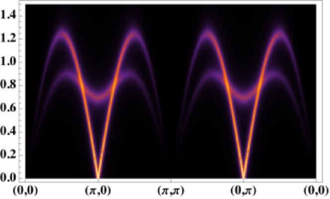
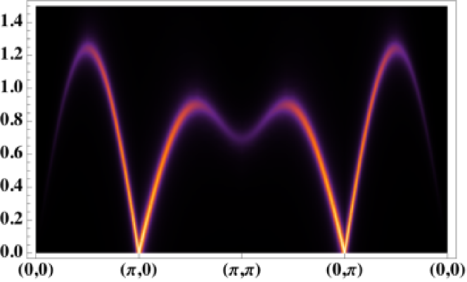
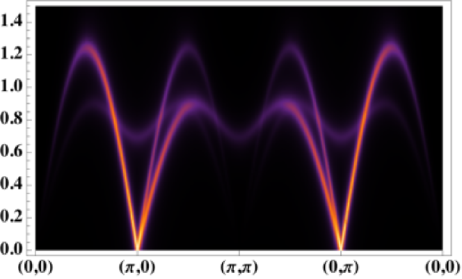
Figure 7: The structure factors $\mathcal{S}_{xx}=\mathcal{S}_{zz}$ (top panel), $\mathcal{S}_{yy}$ (mid panel) and $\mathcal{S}=\sum_{i}\mathcal{S}_{ii}$ (bottom panel) for the orthomagnetic phase. The vertical axis is the energy measured in units of $4J_{2}S$, whereas the horizontal axis displays momentum cuts in the Fe-square-lattice Brillouin zone. The parameters used here are $J_{1}=0.8J_{2}$ and $K=-0.1J_{2}$. Two gapless spin-wave branches emerge from the ordering vectors $\mathbf{Q}_{1}=\left(\pi,0\right)$ and $\mathbf{Q}_{2}=\left(0,\pi\right)$, in sharp contrast to the case of domains of stripes shown in Fig. 6.

IV Discussion and conclusions

We investigated in details under what conditions the orthomagnetic state, which displays a non-collinear double-$\mathbf{Q}$ tetragonal magnetic structure, becomes the magnetic ground state of the iron pnictides within a microscopic itinerant model. We found that large deviations from perfect nesting favor a tetragonal magnetic state, but do not select between the non-collinear and non-uniform configurations – Figs. 1(c) and (d), respectively. Instead, the non-collinear order is favored by the residual electronic interactions that do not participate in the SDW – in agreement with the results found in Ref. Eremin10 – whereas the non-uniform state is favored by coupling to soft Neel-like fluctuations, as discussed by two of us in Ref. xiaoyu . Our investigation is complementary to previous works reporting that different regions of the large parameters space of the iron-based superconductors may display magnetic ground states that do not break tetragonal symmetry Lorenzana08 ; Eremin10 ; Brydon11 ; xiaoyu . In particular, Ref. avci showed that the same three-band model studied in Section II accounts for a transition inside the magnetic stripe state to the $C_{4}$-magnetic state. Our findings reveal that the tetragonal magnetic state can also appear as the primary magnetic instability of the system, without requiring pre-existing stripe order.

The significance of the observation of tetragonal magnetic states in $\text{Ba}(\text{Fe}_{1-x}\text{Mn}_{x})_{2}\text{As}_{2}$, $(\text{Ba}_{1-x}\text{K}_{x})\text{Fe}_{2}\text{As}_{2}$, and $(\text{Ba}_{1-x}\text{Na}_{x})\text{Fe}_{2}\text{As}_{2}$ relies on its implication to the nature of the magnetism of these materials. First, the existence of magnetic Bragg peaks at $\mathbf{Q}_{1}=\left(\pi,0\right)$ and $\mathbf{Q}_{2}=\left(0,\pi\right)$ in the absence of a splitting of the lattice Bragg peaks implies that the tetragonal symmetry-breaking is not a prerequisite for the formation of magnetic order, challenging the point of view that ferro-orbital order is the leading normal-state instability. Furthermore, because the non-collinear and non-uniform magnetic states do not belong to the ground state manifold of the $J_{1}$-$J_{2}$ model, the latter is likely not the most suitable low-energy model to describe the magnetic properties of the iron-based superconductors.

Of course, these statements rely on the confirmation that $\text{Ba}(\text{Fe}_{1-x}\text{Mn}_{x})_{2}\text{As}_{2}$, $(\text{Ba}_{1-x}\text{K}_{x})\text{Fe}_{2}\text{As}_{2}$, and $(\text{Ba}_{1-x}\text{Na}_{x})\text{Fe}_{2}\text{As}_{2}$ do display tetragonal magnetic order. Up to now, the observations have focused on the absence of detectable structural distortion, which is usually large in most iron-based materials kim due to their sizable magneto-elastic coupling Patz14 . Nevertheless, given the resolution limitations intrinsic to x-ray and neutron diffraction probes inosov , it is desirable to find other signatures of these tetragonal magnetic states. Here, we have shown how qualitative features in the spin-wave spectrum can unambiguously distinguish between the stripe and orthomagnetic (non-collinear) phases. For instance, while the latter displays two anisotropic gapless spin-wave branches emerging from each of the ordering vectors $\mathbf{Q}_{1}=\left(\pi,0\right)$ and $\mathbf{Q}_{2}=\left(0,\pi\right)$, a system with domains of the two distinct stripe states displays a single gapless spin-wave branch emerging from each of them. Furthermore, only in the orthomagnetic phase the spin waves can also be detected in off-diagonal components of the spin-spin correlation function. These two distinguishing features can in principle be probed by unpolarized and polarized neutron scattering experiments, respectively. We have not discussed the spin-wave spectrum of the non-uniform phase, which is beyond the scope of the current paper. Yet, because this state is collinear, one does not expect the appearance of additional Goldstone modes, as in the orthomagnetic phase. Interesting features can appear at the ordering vector $\mathbf{Q}_{1}+\mathbf{Q}_{2}=\left(\pi,\pi\right)$ in the non-collinear phase due to the formation of a composite order parameter, as discussed in Ref. xiaoyu . It remains to be seen how these tetragonal magnetic states affect the superconducting state.

Finally, we note that the results obtained here for the spin-wave spectra of the stripe and orthomagnetic phases can also be useful to determine the magnetic states of other compounds that display magnetic Bragg peaks at $\mathbf{Q}_{1}=\left(\pi,0\right)$ and $\mathbf{Q}_{2}=\left(0,\pi\right)$ but no orthorhombic distortion. In general, without knowledge of the size of the magneto-elastic coupling, it is difficult to establish whether these observations are consistent with domains of stripes or orthomagnetic order. A recent example is the compound GdRhIn₅, which is related to the 115 family of heavy fermions granado . Although resonant x-ray scattering found evidence for magnetic order at momenta $\mathbf{Q}_{1}$ and $\mathbf{Q}_{2}$, synchrotron x-rays were unable to resolve a structural distortion. Furthermore, the magnetic transition seems to be second-order, which is difficult to reconcile with a simultaneous structural transition. An interesting alternative would be the formation of an orthomagnetic state, which could be identified by neutron scattering experiments deep inside the magnetically ordered state.

V Acknowledgements

We thank A. Böhmer, P. Canfield, M. Chan, A. Chubukov, I. Eremin, A. Goldman, M. Greven, C. Meingast, R. McQueeney, R. Osborn, P. Pagliuso, L. Taillefer, and G. Yu for fruitful discussions. This work was supported by the U.S. Department of Energy under Award Number DE-SC0012336.

Appendix A Contribution of the residual interactions to the free energy

Here we show how to explicitly compute the contribution of the residual interactions $U_{2}$, $U_{4}$, $U_{5}$, $U_{6}$, $U_{7}$, and $U_{8}$ in Eq. (3) to the free energy. We illustrate the procedure by considering the $U_{7}$ term, corresponding to an exchange-like interaction between the electron pockets at $\mathbf{Q}_{1}$ and $\mathbf{Q}_{2}$. To lowest order in $U_{7}$, the contribution to the free energy corresponds to the two Feynman diagrams shown in Fig. 3 in the main text. Because we are interested in the uniform limit of the action, the momentum of the fields $\mathbf{M}_{1}$ and $\mathbf{M}_{2}$ is set to zero. Also, because we are approaching the transition from the paramagnetic side, we ignore the corrections to the electronic Green’s functions due to the presence of SDW order.

Denoting the generalized momentum by $q$, the left diagram corresponds to

$$U_{7}\left(M_{1}^{i}M_{2}^{l}M_{2}^{j}M_{1}^{k}\right)\left(\sigma_{\alpha\mu}^{i}\sigma_{\mu\alpha}^{l}\sigma_{\beta\nu}^{j}\sigma_{\nu\beta}^{k}\right)$$

$$\left[G_{h}\left(q\right)G_{e_{1}}\left(q\right)G_{e_{2}}\left(q\right)G_{h}\left(p\right)G_{e_{1}}\left(p\right)G_{e_{2}}\left(p\right)\right]$$ (52)

where $i,j,k,l$ correspond to vector components and repeated index are implicitly summed. The sum over Pauli matrices is equivalent to:

$$\text{Tr}\left\{\sigma^{i}\sigma^{l}\right\}\text{Tr}\left\{\sigma^{j}\sigma^{k}\right\}=4\delta^{il}\delta^{jk}$$ (53)

As a result, this diagram gives the contribution

$$4U_{7}\left(\sum G_{h}G_{e_{1}}G_{e_{2}}\right)^{2}\left(\mathbf{M}_{1}\cdot\mathbf{M}_{2}\right)^{2}$$ (54)

The right diagram corresponds to:

$$-U_{7}\left(M_{1}^{i}M_{2}^{l}M_{2}^{j}M_{1}^{k}\right)\left(\sigma_{\mu\beta}^{i}\sigma_{\beta\nu}^{l}\sigma_{\nu\alpha}^{j}\sigma_{\alpha\mu}^{k}\right)$$

$$\left[G_{h}\left(q\right)G_{e_{1}}\left(q\right)G_{e_{2}}\left(q\right)G_{h}\left(p\right)G_{e_{1}}\left(p\right)G_{e_{2}}\left(p\right)\right]$$ (55)

where the minus sign comes from the closed fermionic loop. Using the identity:

Tr$$\left\{\sigma^{i}\sigma^{l}\sigma^{j}\sigma^{k}\right\} \left(\delta^{il}\delta^{jk}-\delta^{ij}\delta^{kl}+\delta^{ik}\delta^{jl}\right)$$=2 (56)

we obtain:

$$\begin{split}&-2U_{7}\left(\sum G_{h}G_{e_{1}}G_{e_{2}}\right)^{2}M_{1}^{2}M_{2}^{2}\\ =&-\frac{U_{7}}{2}\left(\sum G_{h}G_{e_{1}}G_{e_{2}}\right)^{2}\left[\left(\mathbf{M}_{1}^{2}+\mathbf{M}_{2}^{2}\right)^{2}-\left(\mathbf{M}_{1}^{2}-\mathbf{M}_{2}^{2}\right)^{2}\right]\end{split}$$ (57)

All the other terms can be computed in an analogous way.

References

- (1) Y. Kamihara, T. Watanabe, M. Hirano and H. Hosono, J. Am. Chem. Soc. 130, 3296 (2008).
- (2) K. Ishida, Y. Nakai and H. Hosono, J. Phys. Soc. Japan 78, 062001 (2009); D. C. Johnston, Adv. Phys. 59, 803 (2010); J. Paglione and R. L. Greene, Nature Phys. 6, 645 (2010); P. C. Canfield and S. L. Bud’ko, Annu. Rev. Cond. Mat. Phys. 1, 27 (2010); H. H. Wen and S. Li, Annu. Rev. Cond. Mat. Phys. 2, 121 (2011).
- (3) X. Lu, J. T. Park, R. Zhang, H. Luo, A. H. Nevidomskyy, Q. Si, and P. Dai, Science 345, 657(2014).
- (4) E. C. Blomberg, M. A. Tanatar, A. Kreyssig, N. Ni, A. Thaler, Rongwei Hu, S. L. Bud’ko, P. C. Canfield, A. I. Goldman, and R. Prozorov, Phys. Rev. B 83, 134505 (2011).
- (5) R. M. Fernandes, A. V. Chubukov, and J. Schmalian, Nature Phys. 10, 97 (2014).
- (6) P. Dai, J. Hu, and E. Dagotto, Nature Phys. 8, 709 (2012).
- (7) I. Eremin, J. Knolle, R. M. Fernandes, J. Schmalian, and A. V. Chubukov, J. Phys. Soc. Jpn. 83, 061015 (2014).
- (8) M. D. Johannes and I. I. Mazin, Phys. Rev. B 79, 220510(R) (2009).
- (9) W. Z. Hu, J. Dong, G. Li, Z. Li, P. Zheng, G. F. Chen, J. L. Luo, and N. L. Wang, Phys. Rev. Lett. 101, 257005 (2008)
- (10) W.C. Lv, J. Wu and P. Phillips, Phys. Rev. B 80, 224506 (2009)
- (11) C. C. Lee, W. G. Yin, and W. Ku, Phys. Rev. Lett. 103, 267001 (2009).
- (12) R. Applegate, R. R. P. Singh, C.-C. Chen, and T. P. Devereaux, Phys. Rev. B 85, 054411 (2012).
- (13) C. Fang, H. Yao, W.-F. Tsai, J. P. Hu and S. A. Kivelson, Phys. Rev. B 77, 224509 (2008)
- (14) C. Xu, M. Muller, and S. Sachdev, Phys. Rev. B 78, 020501(R) (2008).
- (15) R. M. Fernandes, A. V. Chubukov, J. Knolle, I. Eremin and J. Schmalian, Phys. Rev. B 85, 024534 (2012)
- (16) S. Liang, A. Mukherjee, N. D. Patel, E. Dagotto, and A. Moreo, arXiv:1405.6395
- (17) M. G. Kim, A. Kreyssig, A. Thaler, D. K. Pratt, W. Tian, J. L. Zarestky, M. A. Green, S. L. Bud’ko, P. C. Canfield, R. J. McQueeney, and A. I. Goldman, Phys. Rev. B 82, 220503(R) (2010)
- (18) S. Avci, O. Chmaissem, J. M. Allred, S. Rosenkranz, I. Eremin, A. V. Chubukov, D. E. Bulgaris, D. Y. Chung, M. G. Kanatzidis, J.-P Castellan, J. A. Schlueter, H. Claus, D. D. Khalyavin, P. Manuel, A. Daoud-Aladine, and R. Osborn, Nature Comm. 5, 3845 (2014)
- (19) A. Böhmer, F. Hardy, L. Wang, T. Wolf, P. Schweiss, and C. Meingast, arxiv:1412.7038.
- (20) E. Hassinger, G. Gredat, F. Valade, S. Rene de Cotret, A. Juneau-Fecteau, J.-Ph. Reid, H. Kim, M. A. Tanatar, R. Prozorov, B. Shen, H.-H. Wen, N. Doiron-Leyraud, and L. Taillefer, Phys. Rev. B 86, 140502 (2012).
- (21) X. Wang and R. M. Fernandes, Phys. Rev. B 89, 144502 (2014)
- (22) I. Eremin and A. V. Chubukov, Phys. Rev. B 81, 024511 (2010).
- (23) J. Lorenzana, G. Seibold, C. Ortix, and M. Grilli, Phys. Rev. Lett. 101, 186402 (2008).
- (24) P. M. R. Brydon, J. Schmiedt, and C. Timm, Phys. Rev. B 84, 214510 (2011).
- (25) B. Barbara, M. F. Rossignol, J. X. Boucherle, and C. Vettier, Phys. Rev. Lett. 45, 938 (1980).
- (26) A. Stunault, J. Schweizer, F. Givord, C. Vettier, C. Detlefs, J. X. Boucherle, and P. Lejay, J. Phys.: Condens. Matter 21, 376004 (2009).
- (27) J. Jensen and M. Rotter, Phys. Rev. B 77, 134408 (2008).
- (28) P. S. Normile, M. Rotter, C. Detlefs, J. Jensen, P. C. Canfield, and J. A. Blanco, Phys. Rev. B 88, 054413 (2013).
- (29) J. Jensen and P. Bak, Phys. Rev. B 23, 6180(R) (1981).
- (30) R. S. Fishman and S. H. Liu, Phys. Rev. B 59, 8681 (1999).
- (31) P. Chandra, P. Coleman and A. I. Larkin, Phys. Rev. Lett. 64, 88-91 (1990).
- (32) D. S. Inosov, G. Friemel, J. T. Park, A. C. Walters, Y. Texier, Y. Laplace, J. Bobroff, V. Hinkov, D. L. Sun, Y. Liu, R. Khasanov, K. Sedlak, Ph. Bourges, Y. Sidis, A. Ivanov, C. T. Lin, T. Keller, and B. Keimer, Phys. Rev. B 87, 224425 (2013).
- (33) D. D. Khalyavin, S. W. Lovesey, P. Manuel, F. Kruger, S. Rosenkranz, J. M. Allred, O. Chmaissem, and R. Osborn, arXiv:1409.5324.
- (34) M. Gastiasoro and B. Andersen, Phys. Rev. Lett. 113, 067002 (2014).
- (35) E. Granado, B. Uchoa, A. Malachias, R. Lora-Serrano, P. G. Pagliuso, and H. Westfahl, Jr., Phys. Rev. B 74, 214428 (2006)
- (36) A. V. Chubukov, D. V. Efremov and I. Eremin, Phys. Rev. B 78, 134512 (2008)
- (37) S. Maiti and A. V. Chubukov, Phys. Rev. B 82, 214515 (2010)
- (38) R. Thomale, C. Platt, J. Hu, C. Honerkamp, and B. A. Bernevig, Phys. Rev. B 80, 180505(R) (2009).
- (39) E. Berg, S. A. Kivelson, and D. J. Scalapino, Phys. Rev. B 81, 172504 (2010).
- (40) G. Giovannetti, C. Ortix, M. Marsman, M. Capone, J. Brink and J. Lorenzana, Nat. Comm. 2, 398 (2011).
- (41) M. W. Long and W. Yeung, J. Phys. F: Met. Phys. 17, 1175 (1987).
- (42) J. Knolle, I. Eremin, A. V. Chubukov and R. Moessner, Phys. Rev. B 81, 140506(R) (2010)
- (43) J. Knolle, I. Eremin and R. Moessner, Phys. Rev. B 83, 224503 (2011)
- (44) J. Zhao, D. T. Adroja, D. X. Yao, R. Bewley, S. Li, X. F. Wang, G. Wu, X. H. Chen, J. P. Hu and P. C. Dai, Nature Physics 5, 555(2009).
- (45) L. W. Harriger, H. Q. Luo, M. S. Liu, C. Frost, J. P. Hu, M. R. Norman, and P. C. Dai, Phys. Rev. B 84, 054544 (2011).
- (46) Y. Kamiya, N. Kawashima, and C. D. Batista, Phys. Rev. B 84, 214429 (2011).
- (47) A. Chubukov, E. Gagliano, and C. Balseiro, Phys. Rev. B 45, 7889 (1992).
- (48) E. W. Carlson, D. X. Yao, and D. K. Campbell, Phys. Rev. B 70, 064505 (2004).
- (49) J. T. Haraldsen and R. S. Fishman, J. Phys.: Condens. Matter 21 (2009) 216001
- (50) D. X. Yao and E. W. Carlson, Phys. Rev. B 78, 052507 (2008).
- (51) R. Applegate, J. Oitmaa, and R. R. P. Singh, Phys. Rev. B 81, 024505 (2010).
- (52) A. Patz, T. Li, S. Ran, R. M. Fernandes, J.Schmalian, S. L. Bud’ko, P. C. Canfield, I. E. Perakis, and J. Wang, Nature Comm. 5, 3229 (2014).