Ranking and Selection: A New Sequential Bayesian Procedure for Use with Common Random Numbers

Abstract

We introduce a new concept for selecting the best alternative out of a given set of systems which are evaluated with respect to their expected performances. We assume that the systems are simulated on a computer and that a joint observation of all systems has a multivariate normal distribution with unknown mean and unknown covariance matrix. In particular, the observations of the systems may be stochastically dependent as it is the case if common random numbers are used for the simulation. The main application we have in mind is heuristic stochastic optimization where ‘systems’ are different solutions to an optimization problem with random inputs.

We use a Bayesian setup with an uninformative prior and iteratively allocate a fixed number of simulations based on the posterior distribution of the observations until the ranking and selection decision is correct with a given high probability. We introduce a new simple allocation strategy that is directly connected to the error probabilities calculated before. The necessary posterior distributions can only be approximated, but we give extensive empirical evidence that the error made is well below the given bounds.

Our extensive test results show that our procedure BayesRS uses less simulations than comparable procedures from the literature in different correlation scenarios. At the same time BayesRS needs no additional prior parameters and can cope with different types of ranking and selection tasks.

keywords: Sequential Ranking and Selection,

1 Introduction

We consider ranking and selection of systems based on the average performance of the alternatives. The particular set-up used here is motivated by problems from optimization under uncertainty.

Often in operations research as well as in technical applications the performance of solutions depends on some random influence like market conditions, material quality or simply measurement errors. We shall call such random influences a random scenario. Usually, the aim is then to find a solution with minimal expected costs taken over all scenarios. Let $X_{i}=c(i,Z)$ be the random costs when solution (or ’alternative’) $i$ is applied to the random scenario $Z$. We want to measure the quality of $i$ by its expected costs $\mu_{i}:=\text{{E}\,}c(i,Z)$ taken over all possible scenarios.

Except for particularly simple cases, we will not be able to calculate this expression analytically. Instead, we have to estimate $\text{{E}\,}c(i,Z)$ based on a sample $c(i,z_{1}),\ldots,c(i,z_{n}),$ where $z_{1},\ldots,z_{n}$ are random scenarios. We assume here that simulations are done on a computer, therefore we can identify $z_{1},\ldots,z_{n}$ with the seeds used for the random generator.

Optimization with respect to a simulated cost function is often done by heuristic search methods like genetic algorithms, ant algorithms or cross-entropy optimization (see e.g. Reeves [2010], Dorigo and Stützle [2010], Wu and Kolonko [2014]). Typically, these methods take a relatively small set ${\cal L}:=\{1,\ldots,L\}$ of solutions (a ‘population’) and try to improve the quality of $\cal L$ iteratively. The improvement step usually includes a selection of the best solutions from $\cal L$ with respect to their expected costs $\mu_{i}:=\text{{E}\,}c(i,Z)$. Methods of ranking and selection are therefore widely used in heuristic optimization under uncertainty, see e.g. Schmidt et al. [2006] for an overview. As the $\mu_{i}$ can only be estimated, selection will return sub-optimal solutions with a certain error probability.

The aim of this paper is to develop a strategy that allocates simulation runs to alternatives in such a way that the error probability for the selection of good alternatives is below a given bound.

It is well known, that if observations of different solutions are positively correlated, it is more efficient to use common random numbers (CRN), i.e. to compare the solutions on the same scenario (see e.g. Glasserman and Yao [1992]). Positive correlation in our case roughly means, that if a solution $i\in{\cal L}$ has, for a scenario $z,$ costs $c(i,z)$ that are above average, then costs $c(j,z)$ will tend to be over average for all the other solutions $j\in\cal L$ also. In other words, if some scenario $z$ is relatively difficult (costly) for some solution $i,$ then $z$ will tend to be difficult for all solutions. Similarly, a scenario that has small costs (below average) for one solution will tend to be an easy scenario for all solutions creating smaller costs for all of them. This is the behavior which we would expect for many optimization problems. Therefore, we are interested in ranking and selection strategies that can deal with dependent observation from simulation with CRN.

There are many different approaches to ranking and selection in the literature, we mention only the most prominent ones here. Many papers concentrate on sampling from independent alternatives, see e.g. [Kim and Nelson, 2006a] for an overview and [Kim and Nelson, 2006b] for an advanced sequential method, ${\cal{KN\negthickspace+\negthickspace+}}$ . Other authors allow correlated samples but assume that the correlation structure, i.e. the covariance matrix of the joint distribution is known as e.g. in [Fu et al., 2007], or, in a Bayesian set-up that (part of) the prior distribution is known ([Frazier et al., 2011],[Qu et al., 2012]).

As this may not be the case in realistic applications, many procedures use a two stage approach in which a sample of fixed size $n_{0}$ is taken from all observations in the first stage. The unknown parameters, as e.g. the covariance matrix, are then estimated from the first stage sample. Based on these estimates, the samples in the next stage are allocated to the alternatives. In a pure two-stage procedure, sampling stops after the second stage and ranking and selection is performed as e.g. in Nelson and Matejcik [1995], Chick and Inoue [2001a], Fu et al. [2007] or Peng et al. [2013]. A sequential procedure updates the estimates after each stage and starts a new iteration until the final decision reaches a certain level of quality, see e.g. Kim and Nelson [2006b], Chick and Inoue [2001b] or Qu et al. [2012].

The quality of the final decision may be measured by different functions: the opportunity cost (or linear loss) is the difference between the mean of the selected alternative and the true best value (e.g. Chick and Inoue [2001b], Qu et al. [2012]) whereas the $0-1$-reward function is $1$ if the true value is selected and $0$ if not. Here, a selection may be seen as correct if it is within a $\delta$-distance of the true correct alternative (indifference zone). The expected value of the $0-1$-reward function is the probability of a correct selection (PCS), this is used e.g. in Chick and Inoue [2001b], Fu et al. [2007] or Peng et al. [2013].

Similarly, the sample allocation on a single stage may be determined using the value-of-information (or knowledge gradient) approach, choosing an alternative that promises the largest expected increase in the best mean value after the next observation, this is used e.g. in Frazier et al. [2011] or Qu et al. [2012]. On the other hand, the goal may be to maximize the probability of a correct selection (PCS) given a fixed budget of simulations (Chen et al. [1997],Chen and Lee [2010], Peng et al. [2013] or Fu et al. [2007]). In [Luo et al., 2015] and [Ni et al., 2014] execution of ranking and selection in a parallel environment is discussed and [Lee and Nelson, 2014] extends the scope from Normal distributions to general distributions using a bootstrap approach.

In the present paper, we introduce a new Bayesian procedure for ranking and selection called BayesRS that combines some of the features mentioned above. Observations are assumed to be from a multivariate Normal distribution with unknown mean and covariance matrix, where we use a so-called uninformative prior distribution. In a first stage, $n_{0}$ complete observations from all alternatives are made. Then we continue sampling in a sequential fashion until we are sure that the PCS $\geq 1-\alpha$ for a given $\alpha$. For each iteration we are given a fixed computing budget of $b$ simulations that has to be allocated to the alternatives. The only input parameters therefore are $n_{0},\alpha$ and $b$.

Within our procedure BayesRS we compare two different allocation strategies. The first, GreedyOCBA, is adapted from the optimal computing budget allocation strategy of [Chen et al., 1997], see also [Branke et al., 2007]. It allocates the budget according to the increase in the PCS we can expect, if the whole budget would be given to a single alternative. Our new strategy Dpw uses the dominance probability of a pair $(i,j)$ of alternatives, i.e. the posterior probability that the mean of alternative $i$ is less than the mean of $j$. Dpw allocates simulations such that the dominance probabilities of all pairs relevant for the present ranking and selection task (see below) are increased. As these dominance probabilities were also used by BayesRS for the Bonferroni lower bound of the PCS in the last stage, Dpw may simply re-use these values and allocate the simulations for the present stage.

To determine the dominance probabilities, we need the posterior distribution of the unknown mean. Due to a possibly unequal allocation of the simulation budget we may have incomplete observation for the different alternatives. Our particular sampling scheme (see Section 2.2) guarantees a so-called monotone pattern of missing data, i.e. observations are missing only at the end of the sample. For this case the posterior distribution of the means is known in case the covariance matrix $\bm{\Sigma}$ is given. No such result seems to exist for unknown $\bm{\Sigma}$. We therefore use an approximation that is adapted from the well-studied case of complete observations. Our empirical experiments underline the practicability of this approximation, the errors seem to be well below the bounds we imposed.

Many ranking and selection procedures only work for the selection of the best alternative with minimal (or maximal) mean. Our procedure also works for more general targets as long as they can be defined by pairwise comparison of alternatives, as e.g. determining the $m$ best alternatives and rank them or determine the alternative with median mean.

In our empirical tests we compare the two allocation strategies GreedyOCBA and Dpw in different scenarios. We also compared BayesRS with allocation Dpw to two procedures well-known from the literature, namely ${\cal{KN\negthickspace+\negthickspace+}}$ from Kim and Nelson [2006b] and Pluck from Qu et al. [2012](see also [Qu et al., 2015]). In particular Pluck seems to be similar to our set-up as it is a fully sequential procedure that allows dependent observations and requires only mean and scale matrix of the prior distribution to be known. In our experiments however, our procedure BayesRS seemed to be far superior to both, ${\cal{KN\negthickspace+\negthickspace+}}$ and Pluck.

The main contributions of the present paper are: it introduces a new R&S-procedure that allows for dependent sampling without any prior knowledge of parameters, it uses a general target scheme for the alternatives to be selected and it introduces a new simple, and empirically very efficient allocation rule Dpw that is based on a new approximation of the posterior distributions.

This paper is based on the doctoral thesis Görder [2012]. It is organized as follows. In Section 2 we give the exact mathematical description of the sampling process and our Bayesian model. Technical details about the posterior distribution with missing data are sketched in an Appendix. Section 3 generalizes the concept of ranking and selection of solutions and gives a simple Bonferroni bound for the PCS. A precise definition of our complete ranking and selection algorithm is given in Section 4. In Section 5 we introduce the new allocation rule Dpw and the adapted OCBA procedure GreedyOCBA. We report on extensive empirical tests of our algorithm and its comparison to ${\cal{KN\negthickspace+\negthickspace+}}$ and Pluck in Section 6. Some conclusions are given in the final Section 7.

2 The Mathematical Model

2.1 A Bayesian Environment

Let $\mathcal{L}:=\{1,\ldots,L\}$ denote the fixed set of alternatives. $X_{ik}$ is the $k$-th observation of alternative $i\in\mathcal{L}$. Simulating all of the alternatives from $\mathcal{L}$ with the $k$-th scenario therefore leads to a (column) vector of observations

$$\bm{X}_{\,\mbox{\tiny$\circ$}\,k}:=(X_{1k},\ldots,X_{Lk})^{T},\quad k=1,2\ldots.$$ (2.1)

We assume that for known $\bm{\mu},\bm{\Sigma}$, the sequence $\bm{X}_{\,\mbox{\tiny$\circ$}\,1},\bm{X}_{\,\mbox{\tiny$\circ$}\,2},\ldots$ of observations are independent and identically $\mathcal{N}_{L}(\bm{\mu},\bm{\Sigma})$-distributed. Here, $\mathcal{N}_{L}(\bm{\mu},\bm{\Sigma})$ denotes the $L$-dimensional normal distribution with mean $\bm{\mu}=(\mu_{1},\ldots,\mu_{L})^{T}$ $\in\mathbb{R}^{L}$ and the positive definite $L\times L$ covariance matrix $\bm{\Sigma}$. This model includes the case, where the $L$ alternatives are simulated independently (i.e. with different scenarios), then $\bm{\Sigma}$ is a diagonal matrix. $\bm{\mu}$ and $\bm{\Sigma}$ are assumed to be unknown and we want to extract information about $\bm{\mu}$ from the observations $\bm{X}$. As we assume that the simulations are performed on a computer, we may identify the $k$-th scenario with $z_{k}$, the $k$-th seed for the random generator of the observations.

We take a Bayesian point of view and assume that the unknown parameters $\bm{\mu}$ and $\bm{\Sigma}$ are themselves observations of random variables $W$ and $S$ having a prior distribution with density $\pi(\bm{\mu},\bm{\Sigma})$. We do not assume any specific prior knowledge about the parameters, therefore we shall use the so-called non-informative prior distribution (see DeGroot [2004]) with

$$\pi(\bm{\mu},\bm{\Sigma})\,\propto\,\det(\bm{\Sigma})^{-\frac{\nu_{0}+L+1}{2}}$$ (2.2)

where $\propto$ means that the right hand side gives the density $\pi$ up to some multiplicative constant that does not depend on $\bm{\mu}$ or $\bm{\Sigma}$. $\nu_{0}$ is a so-called hyper-parameter that allows to control the degree of uncertainty about $\bm{\Sigma}$ and is set to $L-1$ in our experiments.

2.2 Iterative allocation of simulation runs

In the first stage, all alternatives are simulated $n_{0}$ times for a fixed number $n_{0}$. From iteration $n_{0}+1$ on, the simulation budget $b$ is allocated sequentially to the alternatives, depending on the observations made so far.This may result in samples with missing data.

We assume the following particular CRN sampling scheme: if in iteration $k>n_{0}$ simulations are allocated to alternative $i$, then these simulations start with scenario (seed) $z_{l_{0}}$, where $l_{0}$ is the smallest number $l$ such that $z_{l}$ has not yet been used for alternative $i$, in other words, $z_{l_{0}-1}$ is the last scenario used for alternative $i$, see the example in Figure 2.1.

Figure 2.1: The first five iterations of a sampling scheme with $L=4,n_{0}=3$ and budget $b=7$. The first $n_{0}=3$ iteration use complete observations, the allocation of the $b$ simulations of the forth iteration are marked in gray, those of the fifth in black. $8$ different scenarios (or seeds) are in use.

This results in samples that may contain different numbers of observations for different alternatives, but values may be missing only at the end of the sample, a so-called monotone pattern of missing data. As this pattern does not depend on the unobserved data (but only on the observed ones via the allocation rule) it is also ignorable, see Schafer [1997] for an exact definition of these terms. Although this may seem rather artificial, it is crucial for the distribution analysis below. It is easily implemented by a suitable book-keeping of the random seeds.

We use

$$\bm{X}_{i\,\mbox{\tiny$\circ$}\,}:=(X_{i1},X_{i2},\ldots,X_{in_{i}})$$ (2.3)

to denote the random (row) vector of the $n_{i}$ (consecutive) observations produced for the $i$-th alternative, $i=1,\ldots,L$, under this scheme and, similarly, $\bm{x}_{i\,\mbox{\tiny$\circ$}\,}:=(x_{i1},x_{i2},\ldots,$ $x_{in_{i}})$ for a specific sample.

Let $\bm{n}=(n_{1},\ldots,n_{L})\in\mathbb{N}^{L}$ be the vector of the present sample sizes for each of the $L$ alternatives, then the variables $\bm{X}_{i\,\mbox{\tiny$\circ$}\,},i=1,\ldots,L,$ can be collected into a matrix-like scheme with possibly different row lengths $n_{i}$ :

$$\bm{X}_{(\bm{n})}:=\bm{X}_{(n_{1},\ldots,n_{L})}:=\begin{pmatrix}X_{11},&X_{12},&\ldots&X_{1n_{1}}\\ X_{21},&X_{22},&\ldots&X_{2n_{2}}\\ \vdots&\vdots&&\vdots\\ X_{L1},&X_{L2},&\ldots&X_{Ln_{L}}\end{pmatrix}.$$ (2.4)

Columns $\bm{X}_{\,\mbox{\tiny$\circ$}\,k}$ may be incomplete for $k>n_{0}$, as the $k$-th scenario or seed may not have been allocated to all alternatives. In the example in Figure 2.1, columns $6,7,8$ are incomplete. Let $\mathbb{R}^{L\otimes\bm{n}}$ denote the set of possible samples $\bm{x}_{(\bm{n})}$ that may be observed with $\bm{X}_{(\bm{n})}$ for a particular size vector $\bm{n}=(n_{1},\ldots,n_{L})$. An allocation rule is a mapping $Q:\mathbb{R}^{L\otimes\bm{n}}\to\mathbb{N}^{L}$ that determines the numbers $q_{1},\ldots,q_{L}$ of additional simulations for each alternative. Then $\bm{n}$ is updated to $\bm{n}^{\prime}:=(n_{1}+q_{1},\ldots,n_{L}+q_{L})$ and the new observations are added at the end of each line of $\bm{x}_{(n)}$ to form the new sample $\bm{x}_{(\bm{n}^{\prime})}$, an element of $\mathbb{R}^{L\otimes\bm{n}^{\prime}}$.

Note, that with this sampling scheme, the simulations in different iterations need not be independent as for some alternatives we may have to re-use scenarios that have already been used in earlier iterations for other alternatives. E.g. in Figure 2.1, the next simulation with alternative $2$ would have to use seed $z_{6}$. This means that we have to keep random seeds until all alternatives have been simulated with this seed. A new seed resulting in an independent observation is used for the simulation of some alternative $i$ only if $n_{i}=\max\{n_{1},\ldots,n_{L}\}$, that is all seeds used so far have been applied to $i$. This would be the case for alternative $1$ in Figure 2.1.

The allocation schemes we use below depend on the posterior distribution of the mean $W$ given data $\bm{x}\in\mathbb{R}^{L\otimes\bm{n}}$ which is determined in the next Subsection.

2.3 Likelihood and posterior distributions with missing data

The likelihood function of incomplete samples as described in the last section are examined in great detail and generality e.g. in Schafer [1997] and Dominici et al. [2000]. Our case is comparatively simple, as our sampling scheme guarantees monotone and ignorable patterns of missing data.

To simplify notation, let the set of alternatives $\mathcal{L}=\{1,\ldots,L\}$ be ordered such that for the present data $\bm{x}=\bm{x}_{(\bm{n})}\in\mathbb{R}^{L\otimes\bm{n}}$ with $\bm{n}=(n_{1},\ldots,n_{L})$ we have

$$n_{1}\geq n_{2}\geq\cdots\geq n_{L}.$$ (2.5)

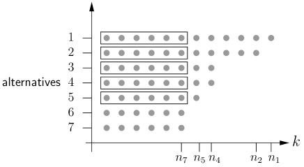
Figure 2.2: A sample with $\mathcal{L}=\{1,\ldots,7\}$ and $n_{1}=12,n_{2}=11,n_{3}=n_{4}=8,n_{5}=7,n_{6}=n_{7}=6$. $\overline{\bm{x}}^{(n_{6})}_{[<6]}$ contains all $5$ sample means from the boxed values.

We need projections of vectors and matrices to components corresponding to subsets of the alternatives $\mathcal{L}=\{1,\ldots,L\}$. For $\bm{y}=(y_{1},\ldots,y_{L})^{T}\in\mathbb{R}^{L}$ and $i\in\{1,\ldots,L\}$ let

$$\bm{y}_{[<i]}:=(y_{1},\ldots,y_{i-1})^{T}\in\mathbb{R}^{i-1},\quad\text{ and }\quad\bm{y}_{[\leq i]}:=(y_{1},\ldots,y_{i})^{T}\in\mathbb{R}^{i}.$$ (2.6)

Similarly, for the $L\times L$ matrix $\bm{\Sigma}=(\sigma_{k,l})_{k,l=1,\ldots,L}$ we define

$$\bm{\Sigma}_{[\leq i]} := (\sigma_{kl})_{k,l=1,\ldots,i},\qquad\bm{\Sigma}_{[<i]}:=(\sigma_{kl})_{k,l=1,\ldots,i-1},$$

$$\bm{\Sigma}_{[i,<i]} := (\sigma_{i1},\ldots,\sigma_{i,i-1})\quad\text{ and}\quad\beta_{i}:=\Sigma_{[i,<i]}\big{(}\Sigma_{[<i]}\big{)}^{-1}.$$ (2.7)

For $1\leq i\leq k\leq L$ we have $n_{i}\geq n_{k}$ and we may define the sample mean of alternative $i$ restricted to the first $n_{k}$ observations

$$\overline{\bm{x}}^{(n_{k})}_{i}:=\frac{1}{n_{k}}\sum_{j=1}^{n_{k}}x_{ij}.$$ (2.8)

Then ${\overline{\bm{x}}}_{i}:=\overline{\bm{x}}^{(n_{i})}_{i}$ is the sample mean of alternative $i$ over all $n_{i}$ observations. See Fig. 2.2 for an illustration of $\overline{\bm{x}}^{(n_{i})}_{[<i]}$.

For the dominance probabilities we need the posterior distribution of $W$ given an incomplete observation $\bm{x}$. We first assume, that the covariance matrix is known and that the uninformative prior $\pi(\mu)\propto 1$ for the mean is used.

Theorem 1.

Let the conditional distribution of (the columns) $\bm{X}_{\,\mbox{\tiny$\circ$}\,k},\ k=1,2,\ldots$, be i.i.d. $\mathcal{N}_{L}(\bm{\mu},\bm{\Sigma})$ distributed given $W=\bm{\mu}$ and $S=\bm{\Sigma}$. Assume that $W$ has the non-informative prior $\pi(\mu)\propto 1$. Let the (possibly incomplete) data $\bm{x}=\bm{x}_{(\bm{n})}\in\mathbb{R}^{L\otimes\bm{n}}$ with $\bm{n}=(n_{1},\ldots,n_{L}),\ n_{1}\geq n_{2}\geq\cdots\geq n_{L}$ be given as described in Section 2.2.

Then the posterior distribution of $W$ given $\bm{X}=\bm{x},S=\bm{\Sigma}$ is an $L$-dimensional Normal distribution $\mathcal{N}_{L}(\bm{\nu},\bm{\Lambda})$ with mean $\bm{\nu}=(\nu_{1},\ldots,\nu_{L})$ where

$$\nu_{1}:={\overline{\bm{x}}}_{1},\qquad\nu_{i}:={\overline{\bm{x}}}_{i}+\beta_{i}(\bm{\nu}_{[<i]}-{\overline{\bm{x}}}_{[<i]}^{(n_{i})})\quad\text{ for }i=2,\ldots,L,$$ (2.9)

and covariance matrix $\bm{\Lambda}:=\bm{\Lambda}_{[\leq L]}$ where

$$\bm{\Lambda}_{[\leq 1]}=\frac{\sigma_{11}}{n_{1}},\qquad\bm{\Lambda}_{[\leq i]}=\left(\begin{array}[]{c|l}\bm{\Lambda}_{[<i]}&\bm{\Lambda}_{[<i]}\ \beta_{i}^{T}\\[3.87495pt] \hline\cr\rule[2.15277pt]{0.0pt}{8.61108pt}\beta_{i}\ \bm{\Lambda}_{[<i]}&\frac{\sigma_{ii}}{n_{i}}+\beta_{i}(\bm{\Lambda}_{[<i]}-\frac{1}{n_{i}}\bm{\Sigma}_{[<i]})\beta_{i}^{T}\end{array}\right)$$ (2.10)

for $i=2,\ldots,L$.

A proof of Theorem 1 is essentially contained in Schafer [1997], it is sketched in the Appendix.

For the case of an unknown covariance matrix $\bm{\Sigma}$ and prior distribution as in (2.2), a factorization of the likelihood is again given in Schafer [1997], but only for a complex parameterization that is described in the Appendix. There seems to be no way to obtain a closed expression for the posterior distribution of $W$ in this case. We therefore use the results of Theorem 1 and replace the unknown $\bm{\Sigma}$ by its estimate, adapting parameters similarly as it is done in the case of complete observations.

For the estimation of $\bm{\Sigma}_{[<i]}=\big{(}\sigma_{kl}\big{)}_{1\leq k,l<i}$ and $\beta_{i}$ we only consider alternatives $1,\ldots,i-1$ that all have sample sizes $\geq n_{i-1}$. We may therefore use the (maximum likelihood) estimates

$$\hat{\sigma}^{(n_{i-1})}_{kl}=\hat{\sigma}^{(n_{i-1})}_{kl}(\bm{x}):=\frac{1}{n_{i-1}}\sum_{m=1}^{n_{i-1}}(x_{km}-{\overline{\bm{x}}}^{(n_{i-1})}_{k})(x_{lm}-{\overline{\bm{x}}}_{l}^{(n_{i-1})})$$ (2.11)

for $1\leq k,l<i$ and $\bm{x}=\bm{x}_{(\bm{n})}$ and put

$$\hat{\bm{\Sigma}}_{[<i]}=\hat{\bm{\Sigma}}_{[<i]}(\bm{x}) := \Big{(}\hat{\sigma}^{(n_{i-1})}_{kl}\Big{)}_{k,l=1,\ldots,i-1}$$ (2.12)

$$\hat{\bm{\Sigma}}_{[i,<i]}=\hat{\bm{\Sigma}}_{[i,<i]}(\bm{x}) := (\hat{\sigma}^{(n_{i-1})}_{i1},\ldots,\hat{\sigma}^{(n_{i-1})}_{i,i-1}),$$

$$\hat{\beta}_{i}=\hat{\beta}_{i}(\bm{x}) := \hat{\bm{\Sigma}}_{[i,<i]}(\hat{\bm{\Sigma}}_{[<i]})^{-1}.$$ (2.13)

Note that $\hat{\bm{\Sigma}}_{[<i]}$ is not necessarily contained in $\hat{\bm{\Sigma}}_{[\leq i]}$ as the estimates use possibly different sample sizes $n_{i-1}$ and $n_{i}$. In (2.13), we have to make sure that $\hat{\bm{\Sigma}}_{[<i]}$ is nonsingular. From Dykstra [1970] it is known that if the sample size $n_{i-1}$ of $\hat{\bm{\Sigma}}_{[<i]}$ fulfills $n_{i-1}>i-1$, then $\hat{\bm{\Sigma}}_{[<i]}$ is positive definite with probability one. This could be guaranteed, if we require for the initial sample size $n_{0}\geq L$ as then $n_{i-1}\geq n_{0}\geq L>i-1$.

We now plug these estimates into the definition of the posterior means and obtain

$$\begin{split}&\hat{\nu}_{1}=\hat{\nu}_{1}(\bm{x}):={\overline{\bm{x}}}_{1},\quad\hat{\nu}_{i}=\hat{\nu}_{i}(\bm{x}):={\overline{\bm{x}}}_{i}+\hat{\beta}_{i}(\hat{\bm{\nu}}_{[<i]}-{\overline{\bm{x}}}_{[<i]}^{(n_{i})})\quad\text{ and }\\ &\hat{\bm{\nu}}(\bm{x}):=(\hat{\nu}_{1},\ldots,\hat{\nu}_{L}).\end{split}$$ (2.14)

The case of $\hat{\bm{\Lambda}}$ is more complicated. To obtain an adequate estimate $\hat{\bm{\Lambda}}$, we first look at the case of complete observations, i.e. with $n=n_{1}=\cdots=n_{L}>L$. Then it is well-known (see e.g. DeGroot [2004], 10.3) that with $\bm{\Sigma}$ known and an non-informative prior distribution for the mean $W$, the posterior distribution of $W$ would be Normal with

mean $$\overline{\bm{x}} \frac{1}{n}\bm{\Sigma}$$ and covariance matrix . (2.15)

If $\bm{\Sigma}$ is unknown with the non-informative prior distribution as in (2.2), the marginal posterior distribution of the mean $W$ in the complete observation case is an $L$-dimensional $\bm{t}$-distribution with $n-L+\nu_{0}$ degrees of freedom,

location parameter $$\overline{\bm{x}} \frac{1}{n-L+\nu_{0}}\hat{\bm{\Sigma}}_{[\leq L]}(\bm{x})$$ and scale matrix (2.16)

(see DeGroot [2004],10.3).

Switching to incomplete observations with known covariance matrix, Theorem 1 tells us that the posterior mean $\overline{\bm{x}}$ of (2.15) has to be replaced by $\bm{\nu}$ and the covariance $\frac{1}{n}\bm{\Sigma}$ of (2.15) has to be replaced by $\bm{\Lambda}$ as in (2.10), reflecting the different sample sizes for each alternative. Note, that for $n=n_{1}=\cdots=n_{L}$, we have $\bm{\nu}=\overline{\bm{x}}$ and $\bm{\Lambda}=\frac{1}{n}\bm{\Sigma}$. In the case of unknown $\bm{\Sigma}$, it therefore seems reasonable to approximate the posterior distribution of the mean $W$ by an $L$-dimensional $\bm{t}$-distribution with $n_{L}-L+\nu_{0}$ degrees of freedom, location parameter $\hat{\bm{\nu}}(\bm{x})$ and a suitable scale matrix $\hat{\bm{\Lambda}}$. The scale matrix $\hat{\bm{\Lambda}}$ should be obtained from $\bm{\Lambda}$ with the $\sigma_{kl}$ replaced by their estimates in a similar fashion as $\frac{1}{n}\bm{\Sigma}$ in (2.15) is replaced by $\frac{1}{n-L+\nu_{0}}\hat{\bm{\Sigma}}$ in (2.16). In particular, in the $i$-th iteration of the recursive definition of $\bm{\Lambda}$ in (2.10), the constant factor $\frac{1}{n-L+\nu_{0}}$ from (2.16) should be replaced by $\frac{1}{n_{i}-L+\nu_{0}}$ as in this step the sample size $n_{i}\geq n_{L}$ is used.

We therefore choose as approximation to the posterior covariance matrix

$$\hat{\bm{\Lambda}}_{[\leq 1]}=\hat{\bm{\Lambda}}_{[\leq 1]}(\bm{x}) :=\frac{\hat{\sigma}^{(n_{1})}_{11}}{n_{1}-L+\nu_{0}},$$ (2.17)

$$\hat{\bm{\Lambda}}_{[\leq i]}=\hat{\bm{\Lambda}}_{[\leq i]}(\bm{x}) :=\left(\begin{array}[]{c|l}\hat{\bm{\Lambda}}_{[<i]}&\hat{\bm{\Lambda}}_{[<i]}\ \hat{\beta}_{i}^{T}\\[3.87495pt] \hline\cr\rule[2.15277pt]{0.0pt}{8.61108pt}\hat{\beta}_{i}\ \hat{\bm{\Lambda}}_{[<i]}&\frac{\hat{\sigma}^{(n_{i})}_{ii}}{n_{i}-L+\nu_{0}}+\hat{\beta}_{i}\ \big{(}\hat{\bm{\Lambda}}_{[<i]}-\frac{1}{n_{i}-L+\nu_{0}}\hat{\bm{\Sigma}}_{[<i]}\big{)}\hat{\beta}_{i}^{T}\end{array}\right)$$ (2.20)

for $i=2,\ldots,L$, and $\hat{\bm{\Lambda}}=\hat{\bm{\Lambda}}(\bm{x}):=\hat{\bm{\Lambda}}_{[\leq L]}(\bm{x})$. As an additional justification for that choice of $\hat{\bm{\Lambda}}$ we may add that for the complete observation case with $n:=n_{1}=\cdots=n_{L}$, our matrix $\hat{\bm{\Lambda}}$ is equal to the scale matrix $\frac{1}{n-L+\nu_{0}}\hat{\bm{\Sigma}}_{[\leq L]}$ as in (2.16), thus $\hat{\bm{\Lambda}}$ generalizes the complete observation case to our situation with incomplete observations. In the sequel, we therefore assume that the posterior distribution of $W$ given $\bm{X}=\bm{x}$ is a $L$-dimensional $\bm{t}$-distribution with $n_{L}-L+\nu_{0}$ degrees of freedom, location parameter $\hat{\bm{\nu}}(\bm{x})$ and scale matrix $\hat{\bm{\Lambda}}$.

The posterior distribution of the mean $W$ is used here to determine the dominance probability $p_{ij}^{\delta}$ of pairs $(i,j)$ of alternatives, this is the posterior probability that alternative $i$ is better than $j$, i.e. the posterior probability of the event $W_{i}\leq W_{j}+\delta$ for an indifference zone parameter $\delta\geq 0$:

$$p_{ij}^{\delta}:=\text{{P}}[W_{i}\leq W_{j}+\delta\mid\bm{X}=\bm{x}]\ =\ \text{{P}}[W_{i}-W_{j}\leq\delta\mid\bm{X}=\bm{x}].$$ (2.21)

Let $G(\cdot\ ;k,a,b)$ denote the distribution function of the one-dimensional $t$-distribution with $k$ degrees of freedom, location parameter $a$ and scale parameter $b$. From the discussion above and standard properties of the multivariate $\bm{t}$-distribution we may then conclude that

$$p_{ij}^{\delta}\approx\ G(\delta;\ n_{L}-L+\nu_{0},\;\hat{\nu}_{i}-\hat{\nu}_{j},\;\hat{\Lambda}_{ii}+\hat{\Lambda}_{jj}-2\hat{\Lambda}_{ij}).$$ (2.22)

The dominance probability $p_{ij}^{\delta}$ of alternative $i$ over alternative $j$ allows to lower bound the PCS for ranking and selection targets that are based on pairwise comparison as they are introduced now.

3 General Ranking and Selection Schemes

3.1 Target and Selection

Our ranking and selection scheme is a generalization of the approach in Schmidt et al. [2006]. We want to select alternatives from the set $\mathcal{L}=\{1,\ldots,L\}$ according to their ranks under some performance measure, in our case the (estimated) mean value. E.g. we want to select the $m$ alternatives with the lowest mean values and rank them as it is required in ant algorithms. We restrict ourselves to such selections that can be determined using pairwise comparisons of alternatives and then apply (2.21) to bound the error probability. We use an abstract concept which is illustrated by some examples below.

We first define a set $A\subset\{1,\ldots,L\}$ of target ranks. We want to select those alternatives that have ranks from $A$ with respect to their estimated mean values. We also determine whether the selected alternatives should be ranked according to these values.

We estimate the unknown means by the present posterior means $\hat{\nu}_{1}(\bm{x}),\ldots$, $\hat{\nu}_{L}(\bm{x})$ and order them as

$$\hat{\nu}_{i_{1}}(\bm{x})<\hat{\nu}_{i_{2}}(\bm{x})<\cdots<\hat{\nu}_{i_{L}}(\bm{x}).$$ (3.1)

This is possible with probability one as we have continuous posterior distributions for which $\text{{P}}[W_{i}=W_{j}\text{ for some }i\not=j\mid\bm{X}=\bm{x}]=0$. We then estimate the ranks of the alternatives by their ranks in (3.1) and select those alternatives that have estimated ranks in the target set $A$, i.e. we select the alternatives

$$B=B(\bm{x}):=\{i_{j}\mid j\in A\},$$ (3.2)

where the $i_{j}$ are taken from (3.1). The probability that this is a correct selection is the posterior probability that the actual ranks of the selected means $W_{l},l\in B$, are those required by the target set $A$, i.e.

$$PCS:=\text{{P}}[\,\{\text{rank}_{W}(W_{l})\mid l\in B\}=A\mid\bm{X}=\bm{x}\,]$$ (3.3)

where $\text{rank}_{\bm{t}}(t_{j})$ denotes the rank of $t_{j}$ within $\bm{t}=(t_{1},\ldots,t_{L})\in\mathbb{R}^{L}$. If it is required that the selected alternatives are also ranked among themselves then (3.3) is replaced by

$$\begin{split}PCS:=\text{{P}}\big{[}\,\{\text{rank}_{W}(W_{l})&\mid l\in B\}=A\text{ and }\\ &W_{j}\leq W_{l}\text{ for }j,l\in B,j<l\ \mid\bm{X}=\bm{x}\,\big{]}\end{split}$$ (3.4)

We restrict ourselves here to target sets that can be described by pairwise comparisons, i.e. we assume that there is a set $\varrho_{AB}$ of pairs from $\mathcal{L}=\{1,\ldots,L\}$ (or, more formally, a binary relation over $\mathcal{L}\times\mathcal{L}$) such that

$$\begin{split}\{\text{rank}_{W}(W_{l})&\mid l\in B\}=A\\ &\iff W_{i}\leq W_{j}\ \text{ for all }(i,j)\in\varrho_{AB}.\end{split}$$ (3.5)

Then (3.3) becomes

$$PCS=\text{{P}}\big{[}W_{i}\leq W_{j}\ \text{ for all }(i,j)\in\varrho_{AB}\mid\bm{X}=\bm{x}\,\big{]}.$$ (3.6)

If an additional ranking is required then $\varrho_{AB}$ must be extended by pairs $(j,l)$ with $j,l\in B$ and $j<l$, see (3.4). The following examples show how these relations $\varrho_{AB}$ may be obtained.

Example 1.

Assume that (3.1) holds.

1. If we want to select the alternative with smallest mean we put $A:=\{1\}$, $B:=\{i_{1}\}$, and $\varrho_{AB}:=\{(i_{1},j)\mid j\in\mathcal{L}-\{i_{1}\}\}$. Then we have

   $$\{\text{rank}_{W}(W_{l})\mid l\in B\}=A \iff W_{i_{1}}\text{ has rank $1$ in }(W_{1},\ldots,W_{L})$$

   $$\iff W_{i_{1}}\leq W_{j}\ \text{ for all }j\not=i_{1},j=1,\ldots,L$$

   $$\iff W_{i}\leq W_{j}\ \text{ for all }(i,j)\in\varrho_{AB}.$$

2. If we want to select the $m$ best (minimal) alternatives for some $m\leq L$, we put $A:=\{1,\ldots,m\}$ and $B:=\{i_{1},\ldots,i_{m}\}$. As characterizing relation we obtain $\varrho_{AB}:=\{(l,j)\mid l\in B,j\in\mathcal{L}-B\}$. Then

   $$\{\text{rank}_{W}(W_{l}) \mid l\in B\}=A$$

   $$\iff W_{i_{1}},\ldots,W_{i_{m}}\text{ have ranks $1,\ldots,m$ in }W_{1},\ldots,W_{L}$$

   $$\iff W_{i_{k}}\leq W_{j}\ \text{ for all }k=1,\ldots,m,j\notin\{i_{1},\ldots,i_{m}\}$$

   $$\iff W_{i}\leq W_{j}\ \text{ for all }(i,j)\in\varrho_{AB}$$

3. If, in addition, the $m$ best alternatives have to be ranked among themselves then we would choose

   $$\varrho_{AB}:=\{(i_{1},i_{2}),(i_{2},i_{3})\ldots,(i_{m-1},i_{m})\}\cup\{(i_{m},j)\mid j\notin B\}.$$

   This includes the case where a complete ranking of the alternatives is required where

   $$\varrho_{AB}:=\{(i_{1},i_{2}),(i_{2},i_{3})\ldots,(i_{L-1},i_{L})\}.$$

4. In a similar fashion $A,B$ and $\varrho_{AB}$ may be defined to select the median or the span of $(\mu_{1},\ldots,\mu_{L})$.

In the iterative procedure below, the posterior means $\hat{\nu}_{1}(\bm{x}),\ldots,\hat{\nu}_{L}(\bm{x})$ have to be determined after each iteration based on the new observations. Therefore, $B$ and $\varrho_{AB}$ have to be re-calculated in each iteration also.

3.2 A Bound for the Probability of a Correct Selection

Based on the characterizing relation $\varrho_{AB}$ we may now derive a simple lower bound of Bonferroni type for the PCS defined in (3.6) with an indifference parameter $\delta\geq 0$ as follows

$$PCS^{\delta} = \text{{P}}\Big{[}W_{i}\leq W_{j}+\delta\text{ for all }(i,j)\in\varrho_{AB}\mid\bm{X}=\bm{x}\Big{]}$$ (3.7)

$$\geq 1-\sum_{(i,j)\in\varrho_{AB}}\text{{P}}\big{[}W_{i}>W_{j}+\delta\mid\bm{X}=\bm{x}\,\big{]}$$

$$= 1-\sum_{(i,j)\in\varrho_{AB}}\big{(}1-p_{ij}^{\delta}\big{)}\ =:LB^{\delta}(\bm{x}).$$

where $p_{ij}^{\delta}$ was defined in (2.21). Note that for these error bounds we need the dominance probabilities for pairs $(i,j)\in\varrho_{AB}$ only.

We now proceed to define our algorithm in full detail.

4 The Algorithm BayesRS

Let the following items be given:

$\mathcal{L}=\{1,\ldots,L\}$ is the set of alternatives, $A\subset\{1,\ldots,L\}$ is the target set of ranks to be selected and possibly ranked, $\alpha\in(0,1)$ is the bound for the error probability, $b\in\mathbb{N}$ is the simulation budget for each iteration and $n_{0}\in\mathbb{N}$ is an initial sample size.

Initialization

:  Observe $\bm{X}_{\,\mbox{\tiny$\circ$}\,j}$ for $j=1,\ldots,n_{0},$ i.e. make $n_{0}$ complete observations and let $\bm{x}$ denote the result.

Determine the posterior means $\hat{\nu}_{j}(\bm{x}),j\in\mathcal{L},$ as in (2.14), the selection $B(\bm{x})$ as in (3.2), relation $\varrho_{AB}$ as in (3.5) and the dominance probabilities $p^{\delta}_{ij},(i,j)\in\varrho_{AB}$, as in (2.22). Finally calculate the lower bound $LB^{\delta}(\bm{x})$ for the PCS as in (3.7).

while

$LB^{\delta}(\bm{x})\ <\ 1-\alpha$ do

• apply an allocation rule $Q$ to the sample $\bm{x}$ to determine the number of additional simulation runs $\bm{q}=(q_{1},\ldots,q_{L}):=Q(\bm{x})$,

• perform $q_{i}$ simulations with alternative $i\in\mathcal{L}$, taking into account the common random numbers scheme as described in Section 2.2, let $\bm{x}$ be the extended data including the new simulation results,

• update the posterior means $\hat{\bm{\nu}}(\bm{x})$, the selection $B(\bm{x})$, the relation $\varrho_{AB}$, the dominance probabilities $p^{\delta}_{ij},(i,j)\in\varrho_{AB}$, and the lower bound $LB^{\delta}(\bm{x})$.

return the present selection $B(\bm{x})$.

In Görder [2012] it is shown that this algorithm terminates if $\delta>0$ and if at least one simulation is allocated to each alternative in each iteration.

5 Allocation strategies

In each of the iterations described in Section 2.2 it has to be decided how many simulations should be performed for each alternative $i\in\mathcal{L}$.

We first look at a modified version of the so-called optimal computing budget allocation (OCBA) strategy introduced by Chen (see for example Chen et al. [2000, 2008], Chen and Lee [2010]). OCBA allocation strategies try to allocate a fixed simulation budget $b\in\mathbb{N}$ in such a way that the expected value of the $PCS$ is maximized. As this is a difficult non-linear optimization problem, see e.g. Chen and Yucesan [2005], most versions of the OCBA solve a substitute problem and try to maximize a lower bound as $LB^{\delta}(\bm{x})$. For larger instances, even this reduced problem can only be solved heuristically, see e.g. [Chen et al., 1996, 1997, Branke et al., 2007].

We adapt this approach to our environment with dependent observations. Let $p_{ij}^{\delta}(q_{i},q_{j})$ be an estimate of the dominance probability from (2.22) with $q_{i}$ and $q_{j}$ additional simulations for alternatives $i$ and $j$. We assume as in [Branke et al., 2007] that the current estimates of the means in $\hat{\nu}_{i}-\hat{\nu}_{j}$ will not be affected substantially by the additional simulations. The degree of freedom $n_{L}-L+\nu_{0}$ of the $t$-distribution will only change if additional simulations are performed with alternative $L$. The effect of additional simulations on the covariance is difficult to foresee, we use a weighted mixture $\Gamma_{ij}$ of the current values $\hat{\Lambda}_{ii},\hat{\Lambda}_{jj},\hat{\Lambda}_{ij}$:

$$\Gamma_{ij}:= \frac{n_{i}}{n_{i}+q_{i}}\hat{\Lambda}_{ii}\,+\,\frac{n_{j}}{n_{j}+q_{j}}\hat{\Lambda}_{jj}$$

$$-2\left[\frac{\hat{\Lambda}_{ii}}{\hat{\Lambda}_{ii}+\hat{\Lambda}_{jj}}\frac{n_{i}}{n_{i}+q_{i}}\,+\,\frac{\hat{\Lambda}_{jj}}{\hat{\Lambda}_{ii}+\hat{\Lambda}_{jj}}\frac{n_{j}}{n_{j}+q_{j}}\right]\hat{\Lambda}_{ij}.$$

and put

$$p^{\delta}_{ij}(q_{i},q_{j}) :=\begin{cases}G\left(\delta;\,n_{L}-L+\nu_{0}\,,\hat{\nu}_{i}-\hat{\nu}_{j},\,\Gamma_{ij}\right)&\text{ if }i,j\not=L\\ G\left(\delta;\,n_{L}+q_{L}-L+\nu_{0}\,,\hat{\nu}_{i}-\hat{\nu}_{j},\,\Gamma_{ij}\right)&\text{ if }i=L\text{ or }j=L\end{cases},$$ (5.1)

and

$$\tilde{LB}^{\delta}(\bm{x};\bm{q})\, :=\,1-\sum_{(i,j)\in\varrho_{AB}}\Big{(}1-p^{\delta}_{ij}(q_{i},q_{j})\Big{)}.$$

We then define a greedy heuristic (GreedyOCBA) similar to Chen and Lee [2010] and Branke et al. [2007]. It assigns additional simulations to an alternative $l$ proportional to the increase in $\tilde{LB}^{\delta}$ if the whole budget was assigned to $l$. With $\bm{e}_{l}$ denoting the $l$-th unit vector, this increase is given by

$$\Delta_{l} :=\tilde{LB}^{\delta}\left(\bm{x};\,b\cdot\bm{e}_{l}\right)-\tilde{LB}^{\delta}(\bm{x},\bm{0})$$ (5.2)

$$=\sum_{\overset{j\in\mathcal{L}:}{(l,j)\in\varrho_{AB}}}\left[p^{\delta}_{lj}(b,0)-p^{\delta}_{lj}(0,0)\right]+\negthickspace\negthickspace\sum_{\overset{i\in\mathcal{L}:}{(i,l)\in\varrho_{AB}}}\left[p^{\delta}_{il}(0,b)-p^{\delta}_{il}(0,0)\right],$$

Note that $p^{\delta}_{il}(0,0)=p^{\delta}_{il}$. Then, GreedyOCBA distributes the simulation budget proportional to the weights $\Delta_{l}$, i.e.

$$q_{l}:=\left\lfloor b\cdot\frac{\Delta_{l}}{\sum_{i=1}^{L}\Delta_{i}}\right\rfloor,\quad l=1,\ldots,L.$$ (5.3)

A remaining budget $R:=b-\sum_{i=1}^{L}q_{i}$ is allocated according to the largest remainder method.

To determine the weights $\Delta_{l}$, we need the dominance probabilities $p_{ij}^{\delta}$ that have been calculated for lower bound $LB^{\delta}$ in the last iteration, but we also need the $2\cdot|\varrho_{AB}|$ probabilities $p^{\delta}_{ij}(b,0)$ and $p^{\delta}_{ij}(0,b),(i,j)\in\varrho_{AB}$. We now introduce a new allocation scheme Dpw (for ’dominance probability weighting’) that works with the $p_{i,j}^{\delta}$ of the lower bound $LB^{\delta}$ only.

For $(i,j)\in\varrho_{AB}$, a small value of $p_{i,j}^{\delta}$ indicates that the assertion of $W_{i}\leq W_{j}+\delta$ needs additional data. We therefore replace the weights from (5.2) by

$$\tilde{\Delta}_{l}:=\max\Big{\{}(1-p^{\delta}_{ij})\frac{\hat{\Lambda}_{ll}}{\hat{\Lambda}_{ii}+\hat{\Lambda}_{jj}}\ \big{|}\ (i,j)\in\varrho_{AB},\ i=l\text{ or }l=j\Big{\}},$$ (5.4)

Here, those alternatives $l$ get a larger weight that (a) are part of a pair $(i,j)\in\varrho_{AB}$ with a small dominance probability $p_{ij}^{\delta}$ and (b) have a relatively large estimated variance $\hat{\Lambda}_{ll}$ compared to their partners, such that $\hat{\Lambda}_{ll}/(\hat{\Lambda}_{ii}+\hat{\Lambda}_{jj})$ tends to be large. In this case, additional simulations with $l$ might decrease the variance and increase the certainty of the dominance relation $(i,j)$. We may even restrict (5.4) to pairs $(i,j)\in\varrho_{AB}$ with dominance probabilities

$$p^{\delta}_{ij}<1-\frac{\alpha}{|\varrho_{AB}|}$$

where $1-\alpha$ is the given lower bound required for the PCS. Hence we drop those pairs $(i,j)$ from (5.4), that give an above average contribution to $LB^{\delta}>1-\alpha$ already. Dpw then allocates the budget proportional to the weights $\tilde{\Delta}_{1},\ldots,\tilde{\Delta}_{L}$ as in (5.3).

In the empirical tests given in the next Section, Dpw performs slightly better than GreedyOCBA on the average though GreedyOCBA is computationally more complex and uses the information from $2|\varrho_{AB}|$ additional dominance probabilities.

6 Computational study

We implemented the algorithm BayesRS and compared its efficiency to other R&S procedures. The main objectives of the study were:

• to compare different allocation strategies within the framework of
  BayesRS, namely GreedyOCBA, Dpw and EqAlloc, the naive equal allocation of the budget to alternatives,

• to show the efficiency of BayesRS and Dpw for different correlations of the observations,

• to compare BayesRS with Dpw to other R&S-strategies from literature, namely ${\cal{KN\negthickspace+\negthickspace+}}$ , see Kim and Nelson [2006b], and Pluck from [Qu et al., 2012].

We measured the performance of the allocation strategies for BayesRS by the average number of simulations each strategy needs until $LB^{\delta}\geq 1-\alpha$, for ${\cal{KN\negthickspace+\negthickspace+}}$ and Pluck this goal had to be adapted. We also checked the empirical PCS, i.e. the relative frequency of correct selections. For the experiments, we implemented the different procedures with the free statistics software R. In Görder [2012] further studies show the efficiency of our allocation strategies in the context of heuristic optimization methods like ant algorithms.

6.1 Test setup

As our methods require normally distributed observations, we generated them by a $\mathcal{N}_{L}(\bm{\mu},\bm{\Sigma})$-random generator for different values of $\bm{\mu}$ and $\bm{\Sigma}$, which, of course, were not known to the R&S-strategies.

Some parameters were fixed: the number of alternatives $L=20$ (other values showed similar behavior), the error probability $\alpha=0.05$ and the indifference zone parameter $\delta=0.05$. The initial sample size was $n_{0}=L=20$, the budget to be allocated in each iteration was $b=10\cdot L=200$ from which at least one simulation was allocated to each alternative in each iteration. The parameter $\nu_{0}$ for the prior probability of the covariance matrix as in (2.2) showed best results in our setup for $\nu_{0}=L-1=19$ and was therefore fixed to this value throughout our tests.

R&S-case	$\bm{\mu}$
Best1	$\mu_{1}=0,\;\;\mu_{2}=\cdots=\mu_{L}=1$
Best10	$\mu_{1}=\cdots=\mu_{10}=0,\;\;\mu_{11}=\cdots=\mu_{L}=1$
Rank10	$\mu_{1}=0,\,\mu_{2}=1,\ldots,\mu_{10}=9,\mu_{11}=\cdots=\mu_{L}=10$

Table 1: Different values for $\mu$ were used in the $\bm{\mu}$ -case “ufc”.

A basic scenario consists of the following four variables that are varied in the tests:

1. We have examined three different R&S-cases : in “Best₁” we want to select the best alternative, i.e. we use a target set $A=\{1\}$ (see subsection 3.1), in “Best₁₀” we want to select the better half of the alternatives ($A=\{1,\ldots,10\}$) and in “Rank₁₀” we also want to rank these ten best alternatives.

2. Also three different $\bm{\mu}$-cases were used: In the unfavorable case “ufc”, $\bm{\mu}$ is adapted to the R&S-case chosen as described in Table 1. In the case “inc”, $\bm{\mu}$ is the increasing sequence $\mu_{1}=0,\mu_{2}=1,\ldots,\mu_{L}=L-1$. In the case “unif”, $\mu_{1},\ldots,\mu_{L}$ are drawn randomly from the interval $[0,100]$ with a minimal distance of at least $\delta$. This is repeated $M_{\mu}:=15$ times, so that 15 simulations with different random $\bm{\mu}$ are performed in the case “unif”.

3. To see how well our method works for different correlations among the observations, we created covariance matrices $\bm{\Sigma}=\big{(}\sigma_{ij}\big{)}_{i,j=1,\ldots,L}$ with a given joint correlation $cor\in\{0.0,0.2,0.5,0.7,0.9\}$. To do so, variances $\sigma_{11},\ldots,\sigma_{LL}$ were chosen uniformly distributed in the interval $[1,10]$, then we put $\sigma_{ij}:=cor\sqrt{\sigma_{ii}\sigma_{jj}}$ for $1\leq i,j\leq L,i\not=j$. To include negative correlations, we complemented the above construction for $cor\in\{-0.9,-0.5,-0.2\}$ with $\sigma_{ij}:=(-1)^{i-j}|cor|\sqrt{\sigma_{ii}\sigma_{jj}}$ resulting in a covariance matrix with alternating positive and negative entries. So we have eight different $\bm{\Sigma}$-cases. For each case, $M_{cov}:=15$ different covariance matrices were constructed.

4. Finally, we distinguished two distribution-cases: in the case “full”, we used the full joint posterior distribution as described above. In the case “marginal”, we simply used the marginal posterior distributions of the alternatives and estimated the posterior means and variances by standard ML-estimators neglecting possible dependencies. This would be correct in the uncorrelated case with $cor=0.0$, but it is a great simplification in the other cases.

All combinations of these parameters result in $3\times 3\times 8\times 2=144$ different scenarios. For each scenario, $M_{cov}:=15$ covariance matrices $\bm{\Sigma}$ were generated according to the $\bm{\Sigma}$-case chosen and, if the $\mu$-case “unif” was used, also $M_{\mu}=15$ random vectors $\bm{\mu}$ were generated. For each pair of $(\bm{\mu},\bm{\Sigma})$ thus chosen, $M=20$ repetitions of the different allocation strategies were performed. The averages from all these trials are given below as mean no. of simulations. We kept track of the random seeds so that all strategies used the same random observations.

6.2 The unfavorable ${\mu}$-case

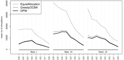
Figure 6.1: The unfavorable ${\mu}$-case: comparison of the allocation strategies EqAlloc, GreedyOCBA and Dpw for all R&S-cases and all $\bm{\Sigma}$-cases.

We first compare the three allocation strategies EqAlloc, GreedyOCBA and Dpw within our algorithm BayesRS. Here, EqAlloc is mainly used to show how difficult the problem instance is. In Figure 6.1 the mean number of simulations necessary to obtain a PCS $\geq 1-\alpha$ with BayesRS and the full posterior distribution is shown. The $x$-axis is divided into the three R&S-cases “Best₁”, “Best₁₀” and “Rank₁₀”, for each of them the results for the eight $\bm{\Sigma}$-cases $cor=-0.9,\ldots,0.9$ are given. The number of simulations on the $y$-axis is the mean over the $M_{cov}=15$ different covariance matrices, each with the given correlation, and the $M=20$ repetitions for each covariance matrix.

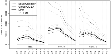
Figure 6.2: The unfavorable ${\mu}$-case: The dotted lines indicate the standard deviation of the results.

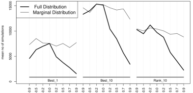
Figure 6.3: The unfavorable ${\mu}$-case: comparison of the results based on full distributions with those using marginal distributions only (BayesRS with allocation Dpw).

Figure 6.1 clearly shows that the intelligent allocation rules are much more efficient than the simple equal allocation. Also in all scenarios, our new allocation rule Dpw performed slightly better than the more classical GreedyOCBA on the average. However, the advantage of Dpw over GreedyOCBA is not significant as can be seen from Figure 6.2 where curves with $\pm$ one standard deviation have been added.

Figure 6.3 compares the two distribution cases for BayesRS with Dpw. The bold curve gives the mean number of observations based on dominance probabilities as given in (2.22) (i.e. case “full”), the light curve are results that are obtained from dominance probabilities based on the marginal distributions of the alternatives only (case “marginal”), neglecting the possible dependencies. Figure 6.3 clearly shows that it is indeed worthwhile to calculate the full posterior distributions in order to save simulations. In particular if observations are positively correlated, the variance of the difference of two alternatives as used in (2.22) is reduced under the full distribution leading to much smaller sample sizes.

The question remains if the reduced sample sizes in the case “full” are large enough to select the right alternatives. We skip the picture of the empirical PCS for this case as it is equal to one for all strategies (except for one case of EqAlloc). This also shows that our assumptions are quite conservative.

6.3 The increasing $\mu$-case

Next we look at the $\bm{\mu}$-case ”inc”, the results are quite similar to the $\bm{\mu}$-case “ufc”. Figure 6.4 shows the mean number of simulations in the “full” distribution case and again, Dpw performs slightly better than GreedyOCBA. The comparison of the two distribution cases “full” and marginal is similar as in the case “ufc”. Figure 6.5 shows that the empirical PCS is well above the required 95%.

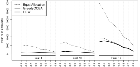
Figure 6.4: $\bm{\mu}$-case “inc”: Comparison of the allocation strategies EqAlloc, GreedyOCBA and Dpw using the full posterior distribution of the unknown means.

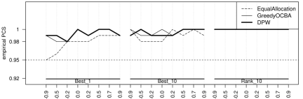
Figure 6.5: $\bm{\mu}$-case “inc”: the empirical PCS of the three different allocation strategies for “full” distribution-case.

6.4 The uniform $\mu$-case

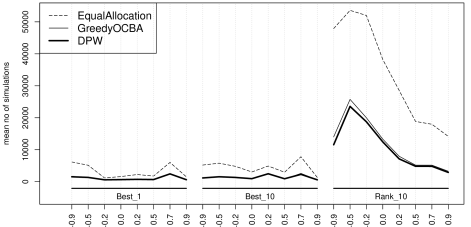
Figure 6.6: $\bm{\mu}$-case “unif”: Comparison of the allocation strategies EqAlloc, GreedyOCBA and Dpw using the full posterior distribution of the unknown means.

In the “unif”-case, results are means over $M_{\mu}=15$ different $\bm{\mu}$ drawn randomly from $[0,100]^{L}$, over $M_{cov}=15$ random covariance matrices and $M=20$ repetitions. To make things comparable, we adapted the indifference zone parameter to $0.05\times\min\{\mu_{i}-\mu_{j}\mid(i,j)\in\varrho_{AB}\}$, i.e. we adapted it to the actual minimal difference appearing in the random mean $\bm{\mu}$.

Results vary considerably depending on the difficulty of $\bm{\mu}$, so that the means give only a rough picture of the performance. Figure 6.6 shows that also for this case our new strategy Dpw is at least as good as GreedyOCBA though it uses less calculations. For the most difficult task ’Rank_10’, the simple EqAlloc could not solve all instances within our limit of 120 000 simulations, therefore it missed the empirical PCS of 95% in some cases.

6.5 Comparison to the procedure ${\cal{KN\negthickspace+\negthickspace+}}$

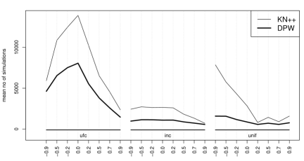
Figure 6.7: Comparison of BayesRS with Dpw and $\cal KN++$ for the R&S-case Best₁. Here, we used a relaxed indifference parameter $\delta_{\text{${\cal{KN\negthickspace+\negthickspace+}}$ }}=0.5$ for ${\cal{KN\negthickspace+\negthickspace+}}$ instead of $\delta=0.05$ as in BayesRS.

In Kim and Nelson [2006b] (see also Kim and Nelson [2006a]) the sequential procedure ${\cal{KN\negthickspace+\negthickspace+}}$ is introduced. It uses a set of active alternatives each of which is simulated once in each iteration. Then, alternatives that are inferior to one of the other active ones are excluded from the active set and from further simulations. The procedure stops as soon as there is only one active alternative left which is then selected as ’best’. The observations for the active alternatives may be correlated but there is no need for re-use of random seeds as the exclusion of alternatives forces a monotone pattern of missing values.

We restricted ourselves to the RS-case Best₁ (target set $A=\{1\}$). ${\cal{KN\negthickspace+\negthickspace+}}$ was allowed to run until only one alternative was left, BayesRS with allocation Dpw used the stopping criterion PCS $\geq 1-\alpha$ as before. In many cases ${\cal{KN\negthickspace+\negthickspace+}}$ could not finish within our limit of 120 000 trials, therefore we biased the set-up in favor of ${\cal{KN\negthickspace+\negthickspace+}}$ : instead of the indifference parameter $\delta=0.05$ it uses $\delta_{\text{${\cal{KN\negthickspace+\negthickspace+}}$ }}=0.5$. Figure 6.7 shows the results. As we have only one RS-case, we collected all three $\bm{\mu}$-cases on the $x$-axis, each with the eight $\bm{\Sigma}$-cases. It turned out that even with an indifference parameter ten times larger, ${\cal{KN\negthickspace+\negthickspace+}}$ needed much more simulations to select the best alternative than BayesRS, in particular in the unfavorable $\bm{\mu}$-case “ufc”. The empirical PCS war almost one for both procedures.

6.6 Comparison to the procedure Pluck

Pluck (projected learning of unknown correlation with knowledge gradients) as defined in Qu et al. [2012] is a fully sequential procedure that allocates just one simulation in each iteration. It aims to select the alternative with the largest mean value, i.e. we have to use target set $A=\{L\}$ in our BayesRS procedure.

Pluck is a Bayesian procedure that assumes a Normal-InverseWishart joint prior distribution for $W$ and $S$, i.e. the conditional distribution of the means $W$, given that $S=\bm{\Sigma}$, is a Normal distribution $\mathcal{N}_{L}(\theta,\bm{\Sigma}/q)$ where $\theta\in\mathbb{R}^{L}$ and $q\in\mathbb{R}$ are known parameters. $S$ has an inverse Wishart distribution with known parameter $\gamma\in\mathbb{R}$ and known scale matrix $\Gamma$. The posterior distribution after the observation of a single alternative is approximated in Qu et al. [2012] by a Normal-InverseWishart distribution which is used as prior distribution for the next iteration. The parameters of this approximation are updates of the prior parameters depending on the single observation in a rather complicated way. In particular, for the posterior update $\gamma^{*}$ of the scalar $\gamma$ a numerical solution to an equation is needed. We replaced this by a rough approximation also mentioned in Qu et al. [2012] and put $\gamma^{*}=\gamma+1/L$.

Instead of maximizing the PCS, Pluck uses the value-of-information approach. In each iteration $n$, it determines the mean $\hat{\theta}_{n}=(\hat{\theta}_{n,1},\ldots,\hat{\theta}_{n,L})$ of the (approximate) posterior distribution of $W$. Then $\Theta_{n}:=\max_{j\in\mathcal{L}}\hat{\theta}_{n,j}$ is the present estimate of the best (in this case largest) unknown mean and the maximizing alternative $j$ is the alternative to be selected in the present iteration. The value of information for an alternative $i$ is the difference between $\Theta_{n}$ and the expectation of $\Theta_{n}$ after an additional simulation has been performed with alternative $i$. The next actual simulation is then allocated to an alternative that has the largest value of information. The performance of Pluck in an experiment is evaluated by the opportunity cost which is the difference between the true largest mean and the mean selected by Pluck.

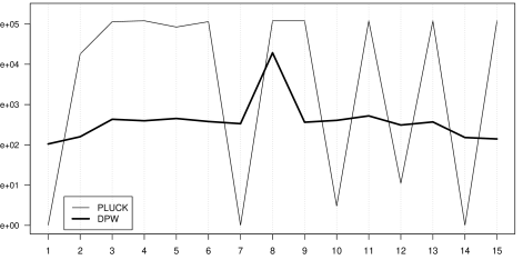
Figure 6.8: The results for the increasing prior mean $\theta=(0,0.2,0.4,\ldots,(L-1)\cdot 0.2)$. Shown are the mean number of simulations for the $15$ random covariance matrices $\bm{\Sigma}$ drawn from an inverse Wishart distribution. Note that the $y$-axis uses a logarithmic scale.

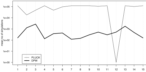
Figure 6.9: The results for the unfavorable prior mean $\theta=(0,\ldots,0,0.2)$. Shown are the logarithms of the mean number of simulations for the $15$ random covariance matrices $\bm{\Sigma}$.

Pluck needs the parameters $\theta,\Gamma,\gamma$ and $q$. To make Pluck comparable to our set-up, we chose as prior parameter $\theta$ the vector determined by our $\bm{\mu}$-case, i.e., as unfavorable, increasing or random, see Subsection 6.1. $\Gamma$ was drawn randomly from a Wishart distribution (with random scale matrix). We set $\gamma=L+1$ and $q=1$ and then simulated the covariance matrix $\bm{\Sigma}$ with an inverse Wishart distribution with parameters $\gamma$ and $\Gamma$. The mean $\bm{\mu}=(\mu_{1},\ldots,\mu_{L})$ is drawn from a Normal distribution $\mathcal{N}_{L}(\theta,\bm{\Sigma})$ (as $q=1$), so that the pair $(\bm{\mu},\bm{\Sigma})$ is drawn from a Normal-InverseWishart distribution as required. In this way, $M_{cov}=15$ pairs $(\bm{\mu},\bm{\Sigma})$ are produced for each of the $\bm{\mu}$-cases “ufc” and “inc”. For the case “unif”, we repeated these steps for the $M_{\mu}=15$ randomly drawn values of $\theta$. Then, simulations were repeated $M=20$ times as before.

Given a pair $(\bm{\mu},\bm{\Sigma})$, the observations $\bm{X}$ are drawn from a Normal distribution $\mathcal{N}_{L}(\bm{\mu},\bm{\Sigma})$ as before. For Pluck, the single samples for each iteration are independent of each other, whereas for BayesRS we used the sampling scheme as described in 2.2.

We continued the iterations in Pluck until the opportunity cost was smaller then the indifference parameter $\delta=0.05$. For our procedure BayesRS with allocation strategy Dpw we assumed an uninformative prior as before and ran it until PCS $\geq 1-\alpha$. This means that Pluck was allowed to know when it hit the true value whereas BayesRS had to ensure PCS $\geq 1-\alpha$.

It turned out, that these test cases were too simple, Pluck selected the true value after one or two steps in most cases, though in some cases it could not find a solution within our limits of $120\,000$ observations. BayesRS had to make the minimal number of $n_{0}=20$ complete observations before it could start. Still on the average, BayesRS was much better due to the few outliers of PLUCK with $120\,000$ observations.

To obtain a more reliable comparison, we restricted ourselves to the prior distributions that were formed after the $\bm{\mu}$-cases ”inc” and ”ufc”. To make these more difficult, we changed the priors from $(0,1,2,\ldots,L-1)$ and $(0,\ldots,0,1)$ to $(0,0.2,0.4,\ldots,(L-1)\cdot 0.2)$ and $(0,\ldots,0,0.2)$, i.e. we decreased the step-size from $1$ to $0.2$ to make the true means more difficult to distinguish. At the same time, we extended BayesRS by computing the exact posterior distributions during the first $n_{0}$ complete observations (using DeGroot [2004],10.3) and stopped when PCS $\geq 1-\alpha$. This is a useful extension for very simple cases.

Figures 6.8 and 6.9 show the results for these two cases. Here the averages over $M=20$ repetitions for each of the randomly drawn $M_{cov}=15$ covariance matrices $\bm{\Sigma}$ is given. As can be seen, in some cases Pluck found the true solution in a single step, whereas in most others, it could not find it within the limit of $120\,000$ observations. Consequently, the empirical PCS was $0$ for these cases, whereas our BayesRS had PCS $\geq 0.95\%$ and even PCS $=1$ in almost all cases. Probably, Pluck is more suited for a larger number of alternatives, where the opportunity cost has more meaning than in our case.

7 Conclusion and future work

In this paper we presented a new sequential Bayesian R&S procedure with support for common random numbers. Based on an approximation of the posterior distribution of the unknown mean and covariance, the simulation effort could be allocated to alternatives for which insufficient data were available for a pairwise comparison.

Extensive experiments showed the practicability of this approach. In particular, it proved superior to the strategy Pluck that also tries to evaluate the posterior distributions but uses only one trial in each iteration and might get stuck in case the (known) prior parameters are misleading.

In our future work we will extend this concept to the selection of multivariate parameters as they occur in multi-criteria optimization problems. Essential parts of this problem were solved in Görder [2012].

Appendix A Derivation of the Posterior Distribution

From Schafer [1997], 5.2.4, (or many other texts on Normal distributions) we see, that if $(X_{1,k},\ldots,X_{L,k})$ is $\mathcal{N}_{L}(\bm{\mu},\bm{\Sigma})$-distributed, then the conditional distribution of $X_{ik}$ given $(X_{1,k},\ldots,X_{i-1,k})=(x_{1,k},\ldots,x_{i-1,k})=:\bm{x}_{[<i,k]}$ is a one-dimensional Normal distribution with mean

$$\tilde{\mu}_{(i-1)}(\bm{x}_{[<i,k]}) :=\mu_{i}+\beta_{i}(\bm{x}_{[<i,k]}-\bm{\mu}_{[<i]})\quad\text{ and variance }$$ (A.1)

$$\tilde{\sigma}_{(i-1)} :=\sigma_{ii}-\beta_{i}\bm{\Sigma}_{[<i]}\beta_{i}^{T}$$

where $\beta_{i}$ was defined in (2.7). This allows to rewrite the density of $\mathcal{N}_{L}(\bm{\mu},\bm{\Sigma})$ as a product of one-dimensional Normal densities with parameters $\big{(}\tilde{\mu}_{(i-1)}(\cdot)$, $\tilde{\sigma}_{(i-1)}\big{)},i=1,\ldots,l$, where for $i=1$ we put $\tilde{\mu}_{(0)}=\bm{\mu}_{1},\tilde{\sigma}_{(0)}=\sigma_{11}$.

Using this re-parameterization, the likelihood function $l(\bm{\mu},\bm{x})$ of $\bm{\mu}$ for a possibly incomplete observation $\bm{X}=\bm{x}$ with $n_{1}\geq n_{2}\geq\cdots\geq n_{L}$ as in Theorem 1 is a product of one-dimensional Normal densities which can be rearranged to (see e.g. Schafer [1997], 6.5)

$$l(\bm{\mu},\bm{x})\propto$$ (A.2)

$$\phi_{1}(\mu_{1};\ {\overline{\bm{x}}}_{1},\sigma_{11}/n_{1})\cdot\prod_{i=2}^{L}\phi_{1}(\mu_{i};\ {\overline{\bm{x}}}_{i}+\beta_{i}(\bm{\mu}_{[<i]}-{\overline{\bm{x}}}_{[<i]}^{(n_{i})}),\tilde{\sigma}_{(i-1)}/n_{i}).$$

If we assume $\bm{\Sigma}$ to be known and use the uninformative prior $\pi(\bm{\mu})\equiv 1$ for $W$, then this likelihood is also the posterior density of $W$ given $\bm{X}=\bm{x}$. It is a density of a $L$-dimensional Normal distribution $\mathcal{N}_{L}(\bm{\nu},\bm{\Lambda})$ and its factors are the conditional densities of $W_{i}$ given $W_{1},\ldots,W_{i-1},\bm{X}$. Using standard properties of the conditional expectation and conditional covariances, the mean $\bm{\nu}$ is obtained as

$$\nu_{1} =\text{{E}\,}[W_{1}\mid\bm{X}=\bm{x}]={\overline{\bm{x}}}_{1}$$

$$\nu_{i} =\text{{E}\,}[W_{i}\mid\bm{X}=\bm{x}]\ ={\overline{\bm{x}}}_{i}+\beta_{i}(\bm{\nu}_{[<i]}-{\overline{\bm{x}}}_{[<i]}^{(n_{i})})\qquad\text{ for }i=2,\ldots,L.$$

which proves (2.9). Similarly, we obtain $\bm{\Lambda}=(\Lambda_{ij})_{1\leq i,j\leq L}$ from

$$\Lambda_{11} =\bm{V}[W_{1}\mid\bm{X}=\bm{x}]=\frac{\sigma_{11}}{n_{1}}$$

$$\Lambda_{ii} =\bm{V}[W_{i}\mid\bm{X}=\bm{x}]$$

$$=\text{{E}\,}\Big{[}\bm{V}[W_{i}|\bm{X},W_{[<i]}]\;\Big{|}\,\bm{X}=\bm{x}\Big{]}+\bm{V}\Big{[}\text{{E}\,}[W_{i}\mid\bm{X},W_{[<i]}]\;\Big{|}\,\bm{X}=\bm{x}\Big{]}$$

$$=\frac{1}{n_{i}}(\sigma_{ii}-\beta_{i}\bm{\Sigma}_{[<i]}\beta_{i}^{T})+\beta_{i}\ \bm{\Lambda}_{[<i]}\ \beta_{i}^{T},\quad\text{ and for $1\leq k<i$ }$$

$$\Lambda_{ki} =\text{cov}\Big{[}W_{k},W_{i}\ \big{|}\ \bm{X}=\bm{x}\Big{]}$$

$$=\beta_{i}\Big{(}\text{cov}[W_{k},W_{l}\ \big{|}\ \bm{X}_{[<i,\,\mbox{\tiny$\circ$}\,]}=\bm{x}_{[<i,\,\mbox{\tiny$\circ$}\,]}]\Big{)}^{T}_{l=1,\ldots,i-1}=\bm{\Lambda}_{[k,<i]}\beta_{i}^{T}.$$

which proves (2.10).

References

- Branke et al. [2007] Jürgen Branke, Stephen E. Chick, and Christian Schmidt. Selecting a Selection Procedure. Management Science, 53(12):1916–1932, 2007. doi: 10.1287/mnsc.1070.0721. URL http://mansci.journal.informs.org/cgi/doi/10.1287/mnsc.1070.0721.
- Chen and Lee [2010] Chun-Hung Chen and Loo Hay Lee. Stochastic Simulation Optimization: An Optimal Computing Budget Allocation. World Scientific Publishing Company, 2010. ISBN 978-981-4282-64-2.
- Chen and Yucesan [2005] Chun-Hung Chen and Enver Yucesan. An alternative simulation budget allocation scheme for efficient simulation. International Journal of Simulation and Process Modelling, 1(1):49–57, 2005.
- Chen et al. [1996] Chun-Hung Chen, Hsiao-Chang Chen, and Liyi Dai. A gradient approach for smartly allocating computing budget for discrete event simulation. In John M. Charnes, Douglas J. Morrice, Daniel T. Brunner, and James J. Swain, editors, Proceedings of the 1996 Winter Simulation Conference, pages 398–405. IEEE, 1996. ISBN 0-7803-3383-7. doi: 10.1109/WSC.1996.873307.
- Chen et al. [2000] Chun-Hung Chen, Jianwu Lin, Enver Yücesan, and Stephen E. Chick. Simulation Budget Allocation for Further Enhancing the Efficiency of Ordinal Optimization. Discrete Event Dynamic Systems, 10(3):251–270, 2000. doi: 10.1023/A:1008349927281. URL http://www.springerlink.com/index/P132U04NM122G459.pdf.
- Chen et al. [2008] Chun-Hung Chen, Donghai He, Michael Fu, and Loo Hay Lee. Efficient Simulation Budget Allocation for Selecting an Optimal Subset. INFORMS Journal on Computing, 20(4):579–595, 2008. doi: 10.1287/ijoc.1080.0268. URL http://joc.journal.informs.org/cgi/doi/10.1287/ijoc.1080.0268.
- Chen et al. [1997] Hsiao-Chang Chen, Liyi Dai, Chun-Hung Chen, and Enver Yücesan. New development of optimal computing budget allocation for discrete event simulation. In Sigrun Andradottir, Kevin J. Healy, David H. Withers, and Barry L. Nelson, editors, Proceedings of the 1997 Winter Simulation Conference, pages 334–341. IEEE, 1997. ISBN 0-7803-4278-X. doi: 10.1109/WSC.1997.640417.
- Chick and Inoue [2001a] Stephen E. Chick and Koichiro Inoue. New Procedures to Select the Best Simulated System Using Common Random Numbers. Management Science, 47(8):1133–1149, 2001a. doi: 10.1287/mnsc.47.8.1133.10229. URL http://mansci.journal.informs.org/cgi/doi/10.1287/mnsc.47.8.1133.10229.
- Chick and Inoue [2001b] Stephen E. Chick and Koichiro Inoue. New Two-Stage and Sequential Procedures for Selecting the Best Simulated System. Operations Research, 49(5):732–743, 2001b. doi: 10.1287/opre.49.5.732.10615. URL http://or.journal.informs.org/cgi/doi/10.1287/opre.49.5.732.10615.
- DeGroot [2004] Morris H. DeGroot. Optimal Statistical Decisions. John Wiley & Sons, 2004. ISBN 0-471-68029-X.
- Dominici et al. [2000] Francesca Dominici, Giovanni Parmigiani, and Merlise Clyde. Conjugate analysis of multivariate normal data with incomplete observations. Canadian Journal of Statistics, 28(3):533–550, 2000. doi: 10.2307/3315963. URL http://doi.wiley.com/10.2307/3315963.
- Dorigo and Stützle [2010] Marco Dorigo and Thomas Stützle. Ant colony optimization: overview and recent advances. In Handbook of metaheuristics, pages 227–263. Springer, 2010.
- Dykstra [1970] Richard L. Dykstra. Establishing the Positive Definiteness of the Sample Covariance Matrix. The Annals of Mathematical Statistics, 41(6):2153–2154, 1970. doi: 10.1214/aoms/1177696719. URL http://projecteuclid.org/euclid.aoms/1177696719.
- Frazier et al. [2011] Peter I Frazier, Jing Xie, and Stephen E Chick. Value of information methods for pairwise sampling with correlations. In Proceedings of the Winter Simulation Conference, pages 3979–3991. Winter Simulation Conference, 2011.
- Fu et al. [2007] Michael C. Fu, Jian-Qiang Hu, Chun-Hung Chen, and Xiaoping Xiong. Simulation Allocation for Determining the Best Design in the Presence of Correlated Sampling. INFORMS Journal on Computing, 19(1):101–111, 2007. doi: 10.1287/ijoc.1050.0141. URL http://joc.journal.informs.org/cgi/doi/10.1287/ijoc.1050.0141.
- Glasserman and Yao [1992] Paul Glasserman and David D. Yao. Some guidelines and guarantees for common random numbers. Management Science, 38(6):884–908, 1992.
- Görder [2012] Björn Görder. Simulationsbasierte Optimierung mit statistischen Ranking- und Selektionsverfahren. Doctoral thesis, in german, TU Clausthal, 2012.
- Kim and Nelson [2006a] S.-H. Kim and B.L. Nelson. Selecting the best system. In Simulation Handbooks in Operations Research and Management Science, chapter 17, pages 501–532. North-Holland, Elsevier, 2006a.
- Kim and Nelson [2006b] Seong-Hee Kim and Barry L Nelson. On the asymptotic validity of fully sequential selection procedures for steady-state simulation. Operations Research, 54(3):475–488, 2006b.
- Lee and Nelson [2014] Soonhui Lee and Barry L Nelson. Bootstrap ranking & selection revisited. In Proceedings of the 2014 Winter Simulation Conference, pages 3857–3868. IEEE Press, 2014.
- Luo et al. [2015] Jun Luo, L Jeff Hong, Barry L Nelson, and Yang Wu. Fully sequential procedures for large-scale ranking-and-selection problems in parallel computing environments. Operations Research, 63(5):1177–1194, 2015.
- Nelson and Matejcik [1995] Barry L Nelson and Frank J Matejcik. Using common random numbers for indifference-zone selection and multiple comparisons in simulation. Management Science, 41(12):1935–1945, 1995.
- Ni et al. [2014] Eric C Ni, Shane G Henderson, and Susan R Hunter. A comparison of two parallel ranking and selection procedures. In Proceedings of the 2014 Winter Simulation Conference, pages 3761–3772. IEEE Press, 2014.
- Peng et al. [2013] Yijie Peng, Chun-Hung Chen, Michael Fu, and Jian-Qiang Hu. Efficient simulation resource sharing and allocation for selecting the best. IEEE Transactions on Automatic Control, 58:1017–1023, 2013. doi: 10.1109/TAC.2012.2215533.
- Qu et al. [2012] Huashuai Qu, Ilya O Ryzhov, and Michael C Fu. Ranking and selection with unknown correlation structures. In Proceedings of the Winter Simulation Conference, page 12. Winter Simulation Conference, 2012.
- Qu et al. [2015] Huashuai Qu, Ilya O Ryzhov, Michael C Fu, and Zi Ding. Sequential selection with unknown correlation structures. Operations Research, 63(4):931–948, 2015.
- Reeves [2010] Colin R Reeves. Genetic algorithms. In Handbook of metaheuristics, pages 109–139. Springer, 2010.
- Schafer [1997] Joseph L Schafer. Analysis of incomplete multivariate data. CRC press, 1997.
- Schmidt et al. [2006] Christian Schmidt, Jürgen Branke, and Stephen E. Chick. Integrating techniques from statistical ranking into evolutionary algorithms. In Franz Rothlauf and Others, editors, Applications of Evolutionary Computing, pages 752–763. Springer Verlag, 2006. doi: 10.1007/11732242\_73. URL http://www.springerlink.com/index/jk184206618h1248.pdf.
- Wu and Kolonko [2014] Zijun Wu and Michael Kolonko. Asymptotic properties of a generalized cross-entropy optimization algorithm. IEEE Transactions on Evolutionary Computation, 18(5):658–673, 2014.