Adsorption at Liquid Interfaces Induces Amyloid Fibril Bending and Ring Formation

Abstract

Protein fibril accumulation at interfaces is an important step in many physiological processes and neurodegenerative diseases as well as in designing materials. Here we show, using $\beta$-lactoglobulin fibrils as a model, that semiflexible fibrils exposed to a surface do not possess the Gaussian distribution of curvatures characteristic for wormlike chains, but instead exhibit a spontaneous curvature, which can even lead to ring-like conformations. The long-lived presence of such rings is confirmed by atomic force microscopy, cryogenic scanning electron microscopy and passive probe particle tracking at air- and oil-water interfaces. We reason that this spontaneous curvature is governed by structural characteristics on the molecular level and is to be expected when a chiral and polar fibril is placed in an inhomogeneous environment such as an interface. By testing $\beta$-lactoglobulin fibrils with varying average thicknesses, we conclude that fibril thickness plays a determining role in the propensity to form rings.

Current address: Cambridge University, Department of Applied Mathematics and Theoretical Physics, Cambridge CB3 0WA, United Kingdom Current address: ETH Zurich, Department of Materials, Laboratory for Interfaces, Soft Matter & Assembly, 8093 Zurich, Switzerland Current Address: Georgetown University, Department of Physics and Institute for Soft Matter Synthesis & Metrology, Washington DC 20057, USA

This document is the unedited Author’s version of a Submitted Work that was subsequently accepted for publication in ACS ©American Chemical Society after peer review. To access the final edited and published work see http://pubs.acs.org/doi/abs/10.1021/nn504249x.

1 Introduction

Polymers exposed to an unfavorable environment can collapse or change shape in order to minimize surface energy ^{1, 2, 3}. Examples of unfavorable environments include a poor solvent or a hydrophilic-hydrophobic interface like the one between water and either air or oil. Examples of conformations driven by such energy minimization are rings, loops, coils, spools, tori/toroids, hairpins or tennis rackets ⁴. In filaments comprising aggregated proteins or peptides, ring formation falls into two main classes: fully annealed rings occasionally observed as intermediate states during protein fibrillation, like in apolipoprotein C-II ⁵ and A$\beta_{1-42}$ ⁶; or ring formation in actively driven systems, where the energy required for filament bending is provided by GTP or ATP ^{7, 8, 9, 10}. Insulin has been shown to form open-ring shaped fibrils when pressure was applied during fibrillation ¹¹, which was explained by an anisotropic distribution of void volumes in fibrils and therefore aggregation into bent fibrils.

We study amyloid fibrils, which are linear supramolecular assemblies of proteins/peptides that, despite a large diversity in possible peptide sequences, show remarkable structural homogeneity. Peptides form $\beta$-sheets that stack, often with chiral registry, to form a filament whose main axis is perpendicular to the $\beta$-strands ^{12, 13}. Fully formed fibrils can consist of one or, more commonly, multiple filaments, assembled into twisted ribbons with a twist pitch determined by the number of filaments in the fibrils ¹. Their high aspect ratio (diameter usually less than $10$ nm, total contour length up to several $\mu$m) leads to liquid crystalline phases in both three (3D) ¹⁵ and two dimensions (2D) ^{16, 17}. Amyloid fibrils were initially studied due to their involvement in many different degenerative diseases such as diabetes II or Parkinson’s disease ¹⁸. However, protein fibrils have recently experienced a surge of interest in potential applications in materials ¹⁹, and functional roles have been identified in biological processes such as hormone storage ²⁰, emphasizing the importance of understanding their structure and properties in 2D.

Here, we present experimental evidence for the development of curved fibrils at interfaces. Semiflexible $\beta$-lactoglobulin fibrils are found to undergo a shape change and passively form open rings upon adsorption to an interface (liquid-liquid or liquid-air). We show that this cannot be described by a simple bending modulus; this bending can instead be understood in terms of a spontaneous curvature induced on symmetry grounds by the chiral and polar nature of the fibril, when interacting with the heterogeneous environment provided by an interface. A comparison of different fibril batches of the same protein shows that the probability of forming rings depends on the average fibril thickness, with batches of thicker fibrils not forming loops. These results imply that flexible non-symmetric bodies embedded in heterogeneous media — such as the physiological environment — can be expected to deform, bend, and twist, depending on the specific surface interaction with the environment. For example, concentration gradients of ions or pH could enhance shape changes necessary for locomotion in flexible nanoswimmers ^{21, 22}, or be used to promote or control self-assembly through shape changes. One could even envision high surface to volume materials such as bicontinuous phases with large length scales being used to process large amounts of flexible shape changers.

2 Results and discussion

2.1 Morphology

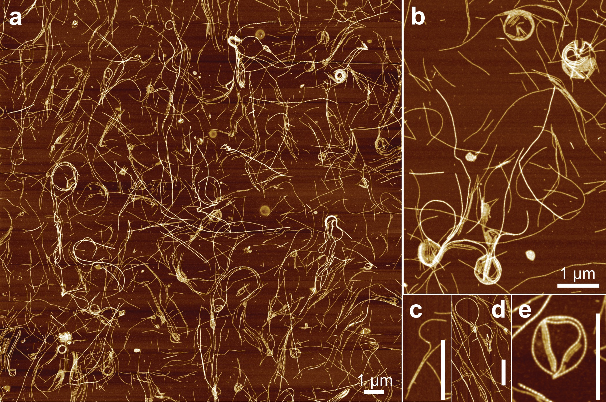
Figure 1: $\beta$-lactoglobulin fibrils form rings and loops at the air-water interface. AFM images of $\beta$-lactoglobulin fibrils at the air-water interface after horizontal transfer onto mica using the Langmuir-Schaefer method. The initial fibril concentration in the bulk was $c_{\text{init}}=0.001\%$ w/w and the waiting time before transfer $t=60$ minutes. The scale bars in c, d, and e correspond to $1$ $\mu$m.

When imaging the air-water interfacial fibril layer by AFM using a modified Langmuir-Schaefer horizontal transfer technique (see Materials and Methods) to resolve 2D liquid crystallinity, we found that, in addition to nematic and isotropic fibril domains ¹⁷, some $\beta$-lactoglobulin fibrils were present in circular conformations. These rings appear at the lowest interfacial density investigated, where fibril alignment is still negligible ¹⁷, and persist in the presence of nematic fibril domains up to high densities [see Supplementary Note 1, Supplementary Fig. S1 and S2]. Ring diameters range from $0.5-2$ $\mu\text{m}$ (Fig. 1 and 2), and are consistent whether observed via AFM at the air-water interface, cryogenic Scanning Electron Microscopy (cryo-SEM) or passive probe particle tracking at the oil-water interface, confirming that fibrils have a similar tendency to bend at air-liquid and liquid-liquid interfaces. A small selection of the vast variety of ring morphologies is presented in Fig. 1. Highly complex structures involving several fibrils are quite common (Fig. 1a, b, S1 and S2), whereas relatively few distinct rings or tennis rackets comprise a single fibril and can rather be thought to be intermediate assembly states $enroute$ to final ring structures (Fig. 1c and d) ²³. Short fibrils, which could be the result of fracture due to the bending strain, exposure to air or inhomogeneous strong surface tension, also assemble into rings (Fig. S3). Alternatively, short fibrils frequently accumulate within an outer ring and align either along the circumference of this ring or parallel to each other in the center, with minimal contact with the ring itself (Fig. 1b and e).

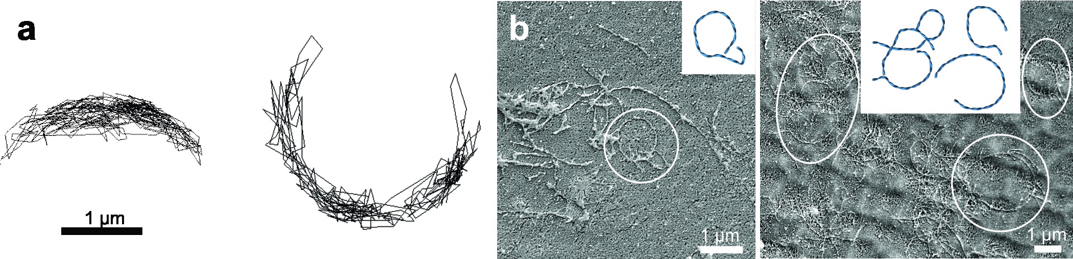
Figure 2: Fibril rings at an oil-water interface. (a) Trajectories of two different silica tracer particles with diameter $\approx{774}$ nm moving around circular obstacles during a passive probe particle tracking experiment of a $c_{\text{init}}=0.005\%$ w/w fibril suspension. The trajectories were isolated $t=24$ and $37$ minutes after interface creation, respectively. The scale bar applies to both trajectories. (b) Cryo-SEM images of the surface of a $c_{\text{init}}=0.001\%$ w/w fibril suspension $t=60$ minutes after medium chain triglycerides (MCT)-water interface creation. The oil phase had been removed by freeze-fracture prior to imaging. Insets show sketches of the rings indicated with circles in the main images.

The long-lived presence, and hence inferred stability, of these self-organized conformations was confirmed by passive probe particle tracking experiments performed at the oil-water interface, where fluorescently-labelled spherical tracer particles (diameter $\approx{774}$ nm) were observed to move in near-perfect circles or sickle-shaped trajectories over the course of three to four minutes. A simple pathway for ring formation could be the presence of nano- or microbubbles at the liquid surface, which give fibrils the opportunity to bend around their circumference ²⁴. This would, however, also lead to a distortion of the peptide layer (see Materials and Methods) at the interface; once the sample has dried, the bubble would have disappeared but still be visible in AFM images as a height discontinuity through the ‘bubble’. The absence of such observations in AFM (Fig. S4), or of bubbles (cavities) in the cryo-SEM images (Fig. 2), indicates that there is an inherent predisposition of the fibrils to bend, which then leads to circle formation upon interaction with a liquid surface.

2.2 Fibril Free Energy

Understanding these data requires a study of how surface effects influence the shape of fibrils (or indeed filaments). We consider an inextensible fibril of length $L$, represented as a twisted ribbon with chiral wavelength $\lambda$ and pitch angle $\theta_{p}=\cot^{-1}(2\pi R/\lambda)$, where $R$ is the inscribing radius of the twisted ribbon (see Supplementary Note 2). We parametrize the shape by $\mathbf{\hat{{t}}}(s)$, the direction parallel to the central axis of the ribbon, or equivalently the tangent vector of the fibril. The ribbon twists around its axis $\mathbf{\hat{{t}}}(s)$ by the angle $\phi(s)$. We will parametrize the bending in terms of the angular rate of deflection $\dot{\boldsymbol{\Theta}}=\mathbf{\hat{{t}}}\times\dot{\hat{\textbf{t}}}$, where $\mathbf{\kappa}(s)=d\mathbf{\hat{{t}}}/ds\equiv\dot{\hat{\textbf{t}}}$ is the local curvature. Hence, $\dot{\boldsymbol{\Theta}}=\kappa\mathbf{\hat{{n}}}$, where $\mathbf{\hat{{n}}}$ is the axis about which the tangent vector is deflected during a bend. For a fibril confined to bend on a surface, we take $\mathbf{\hat{{n}}}$ to be outward surface normal vector (pointing into the liquid), so that $\kappa$ can be either positive or negative. The free energy is given by ²⁵

$$G_{\textrm{fib}} =\int_{0}^{L}ds\left\{\frac{B}{2}{\dot{\Theta}}^{2}+\frac{C}{2}\left(\dot{\boldsymbol{\phi}}-\mathbf{q}\right)^{2}+\mathbf{D}\cdot\dot{\hat{\textbf{t}}}\times(\dot{\boldsymbol{\phi}}-\mathbf{q})\right\}$$ (2.1)

$$=\int_{0}^{L}ds\left\{\frac{B}{2}\,\kappa^{2}+\ldots\right\}.$$ (2.2)

The first term penalizes bending, and $B$ is the bending modulus. The second term penalizes twist relative to the native helical twist, which is parametrized by the chiral wavenumber $q=2\pi/\lambda$. Here, $C$ is the twist modulus. The vector $\mathbf{D}$ represents the twist-bend couplings allowed by a polar fibril with a non-symmetric local cross section ²⁵. In this work we will focus on the bend degrees of freedom, since in filaments with free ends, such as those considered here, the twist degrees of freedom will relax to accomodate any imposed bend.

A polar twisted fibril has an anisotropy that distinguishes ‘head’ from ‘tail’ directions along the fibril axis; in F-actin this ‘polarization’ arises from the orientations required of G-actin monomers to effect self-assembly ²⁶; in an $\alpha$-helix the N-C polymerisation breaks the polar symmetry and in cross-$\beta$ amyloid fibrils such as those studied here the polarity is due to the molecular packing of $\beta$-sheets ^{27, 28, 29}. The polarity is reflected in variations in molecular structure along the exposed surface of the twisted ribbon. When this structure is placed in a heterogenous environment, as occurs near a solid surface or when immersed within a meniscus between two fluids (or fluid and gas), the inhomogeneity of the environment generally leads to unbalanced torques on the body (see Supplementary Note 2, Fig. S5 and S6 for details), even when local forces have balanced to place the fibril at the interface. A non-symmetric body, such as a chiral and polar fibril, can thus experience an effective spontaneous curvature ³⁰.

To demonstrate this effect, we consider a fibril adsorbed onto a planar surface with which it interacts, rather than immersed within a meniscus. The effects are qualitatively the same, but the details are easier to understand in the adsorbed case. The surface and the adsorbed ribbon interact via numerous molecular interactions ³. Although in principle all atoms in the fibril interact with every point on the surface due to Coulomb interactions, screening limits the interaction to only the adsorbing surface. Long-range dispersion interactions are also irrelevant for fibrils that are induced to bend or twist within the plane, since the change in this energy will be negligible. Hence, we consider the following surface free energy

$$G_{\textrm{surf}} =\frac{2L}{\lambda}\int_{S}\left[\bar{\gamma}+\delta\gamma(\mathbf{r})\right]d^{2}r,$$ (2.3)

where $\lambda$ is the twist pitch or wavelength, the average surface energy $\bar{\gamma}$ controls adsorption, and $S$ is the contact area of a the ribbon, which occurs every half wavelength. The asymmetry $\delta\gamma(\mathbf{r})$ reflects the polar nature of the interaction and can vary from repulsive to attractive along the repeat patch. A polar moment (with dimensions of energy) of the interaction can be defined by

$$\mathbf{P}=\frac{2}{\lambda}\int_{S}\,\mathbf{r}\,\delta\gamma(\mathbf{r})\,d^{2}r,$$ (2.4)

where $S$ is the area of the patch where the fibril contacts the surface. The polar moment $\mathbf{P}$ is determined by the nature of the interaction with the surface, and is thus not an intrinsic property of the fibril alone. Fig. 3 shows an example in which the surface patch is a parallelogram with length $\ell$ and width $\omega$. For a simple surface potential $\delta\gamma(\mathbf{r})=\varepsilon(x\cos\Phi+y\sin\Phi)$, where the coordinate $x$ is parallel to the fibril axis coordinate $s$, the polar moment (see Supplementary Note 2) has magnitude $P=\alpha(\theta_{p},\Phi)\omega^{3}\ell\varepsilon/\lambda$. Here, $\alpha(\theta_{p},\Phi)$ is a geometric prefactor whose sign depends on the polarization and chirality, and parametrizes the degree to which the symmetric parellelogram is deformed into a non-symmetric shape to favor one sign of surface ‘charge’.

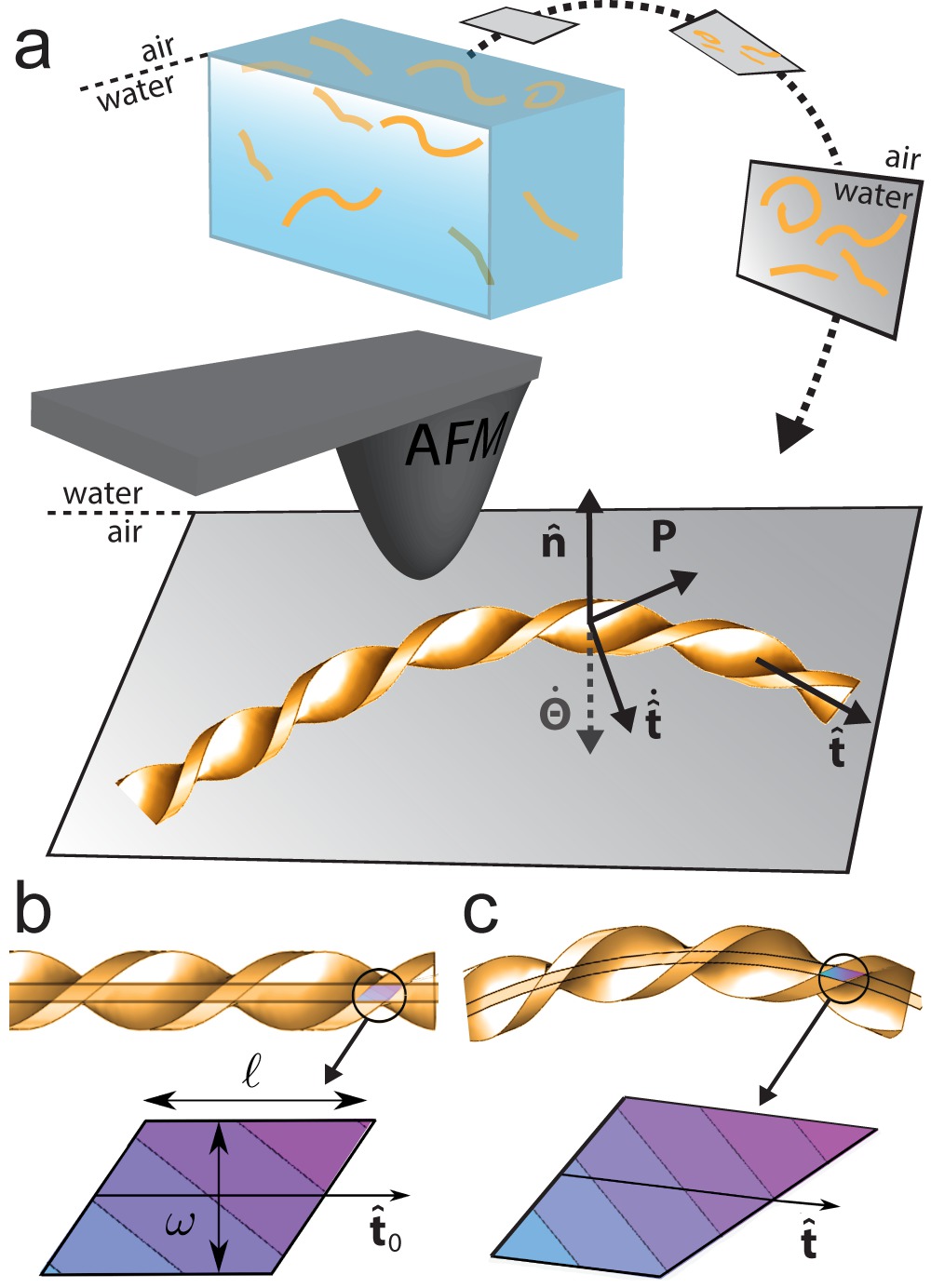
Figure 3: Twisted ribbon against a surface. (a) After horizontal transfer of the interfacial fibril layer, the AFM tip probes the fibrils from the side that was originally pointing towards the water phase. (b, c) The contact area as seen through the interface from the air-side is a parallelogram (b), which deforms asymmetrically when the fibril is bent (c). This leads to a greater contact area by one ’charge’ (indicated by color) of the polar interaction, which implies a preference for one sign of bend and thus a spontaneous curvature. The example shown is that of a bend that decreases the contact energy. The symmetry breaking of the polar region upon bending has been amplified for visualisation purposes.

When the twisted ribbon is bent the ribbon-surface contact area changes shape, so that either the repulsive or attractive part of the polar interaction has more contact with the surface, depending on the sign of the bend (Fig. 3c). This leads to a spontaneous curvature. The contribution of bending to the overall interaction energy can then be written as a chiral coupling between the bending rate $\dot{\boldsymbol{\Theta}}$ and the polar moment $\mathbf{P}$:

$$G_{\textrm{surf}} =\int_{0}^{L}\!\!ds\left\{-{A}\,\dot{\boldsymbol{\Theta}}\cdot\mathbf{\hat{{t}}}\times\mathbf{P}+\ldots\right\}$$ (2.5)

$$=\int_{0}^{L}\!\!ds\left\{-{A}\,\kappa\,\mathbf{\hat{{n}}}\cdot\mathbf{\hat{{t}}}\times\mathbf{P}+\ldots\right\}.$$ (2.6)

The vector product is the simplest term which has no mirror symmetry, and is thus appropriate for a chiral filament. Moreover, under $s\rightarrow-s$ both $\kappa$ and $\mathbf{t}$ change sign, whereas $\mathbf{P}$ does not, so that the free energy is also reparametrization-invariant. The dimensionless geometric factor ${A}$ and the moment $\mathbf{P}$ depend on the details of the surface free energy $\delta\gamma(\mathbf{r})$ interaction potential $U$, the contact area shape, and its deformation under bending. The polar moment $\mathbf{P}$ depends on the surface normal vector through its vector nature and the details of the surface-fibril interaction. The ellipses indicate other terms induced by the surface, such as contributions to the bend-twist or curvature moduli, or a spontaneous twist. We choose the convention that the surface normal vector $\mathbf{\hat{{n}}}$ points away from the surface and thus into the fibril. An example free energy $G_{\textrm{fib,P}}$ is calculated in the Supplementary Information for a simple model contact potential.

The curvature in Eq. 2.6 carries a sign: for $\kappa>0$ the fibril bends in a right-handed sense around the surface normal vector $\mathbf{\hat{{n}}}$, while for $\kappa<0$ the fibril bends in a left-handed sense. The process of transferring the surface layer for AFM observation orients the surface normal towards the AFM observer, so that observation is from the liquid side towards the air side (Fig. 3). Consider a polarization such that $\mathbf{P}\cdot\mathbf{\hat{{y}}}=\sin\Phi$, where $\Phi=+\pi/4$, and choose $\mathbf{\hat{{t}}}\parallel\mathbf{\hat{{x}}}$ (as observed in the AFM image; see Fig. 3), where $\mathbf{\hat{{x}}}\times\mathbf{\hat{{y}}}=\mathbf{\hat{{n}}}$. This implies $\mathbf{\hat{{n}}}\cdot{\mathbf{\hat{{t}}}}\times\mathbf{\hat{{P}}}>0$. Consider a bend as shown in Fig. 3, in which $\dot{\boldsymbol{\Theta}}\cdot\mathbf{\hat{{n}}}=\kappa$, where $\kappa<0$. In Supplementary Note 2 we find ${A}>0$, so that this bend ($\kappa<0$) increases the energy, and thus $\kappa>0$ is favored. Similarly, for the opposite sign of $\mathbf{\hat{{t}}}\times\mathbf{P}$ a negative curvature $\kappa<0$ is favored.

The competition between the surface energy (Eq. 2.6) and the ordinary fibril bending energy (Eq. 2.1) leads, by minimization, to a spontaneous curvature $\kappa_{0}$ given by (see SI)

$$\kappa_{0}=\frac{{A}}{B}\,\mathbf{\hat{{n}}}\cdot\mathbf{\hat{{t}}}\times\mathbf{P}.$$ (2.7)

This is equal to $\varepsilon\omega^{3}\ell\,\alpha(\theta_{p},\Phi)/B\,\lambda\sin^{2}\theta_{p}$ for the simple surface potential $\delta\gamma(\mathbf{r})=\varepsilon(x\cos\Phi+y\sin\Phi)$. Isambert and Maggs ³⁰ articulated how a surface can induce spontaneous curvature in a polar and chiral filament. They proposed a phenomenological free energy with an explicit spontaneous curvature that depends on the twist angle, and a surface interaction that breaks polar symmetry. Hence, they have actually introduced a spontaneous curvature ‘by hand’. Conversely, we present a model in which a polar surface interaction is itself chiral by virtue of the local chirality of the filament, and this gives rise to an effective spontaneous curvature as a result of total energy minimization. Therefore, the functional form of the resulting spontaneous curvature differs from that proposed in Ref. [30].

Enhanced curvature is expected for amyloid fibrils with fewer filaments (as confirmed in Fig. 5), which will have smaller bending moduli $B$, or for fibrils with larger polar moments $P$ and thus stronger surface interactions. In addition, the specific details of the surface deformation encapsulated in the function $\alpha(\theta_{p},\Phi)$ play an important role: fibrils for which the deformation leads to a more symmetric contact area will have a stronger geometric factor and thus a greater expected spontaneous curvature.

2.3 Non-Gaussian Curvature Distributions

Consider a segment of arc length $ds$ of a wormlike chain (WLC). The probability ${\cal P}(\kappa)$ of finding this segment curved with curvature $\kappa=1/R_{\kappa}$, where $R_{\kappa}$ is the radius of curvature, is governed by the bending modulus and should be Gaussianly distributed, ${\cal P}(\kappa)\sim\exp\left\{-ds\,\ell_{p}\kappa^{2}/2\right\}$, where $\ell_{p}=B/k_{\scriptscriptstyle\rm B}T$ is the persistence length. Deviations from the WLC model can be quite common, as with toroidal DNA ^{32, 33}, in which the nucleic acids have a smaller persistence length at short length scales ³². The presence of rings in our system suggests a characteristic intrinsic curvature or length scale, in addition to the usual $\ell_{p}$. For quantitative analysis, we have extracted the $xy$ coordinates of fibrils from images acquired at low interfacial fibril densities after short adsorption times, where interactions and contact between fibrils are still minimal, and calculated ${\cal P}(\kappa)$ (Fig. 4; see Materials and Methods). Any rings present on the image were excluded from the analysis, since their closed topology would introduce an additional constraint. To benchmark this approach, we first generate conformations based on the discrete WLC model with the $\ell_{p}$ obtained from the 2D mean squared end-to-end distance of fibrils at the air-water interface ³⁴. These conformations are used to create artificial images of WLC polymers with the same resolution as the AFM images and then subjected to the same tracking algorithm used for analyzing the real fibril image. Fig. 4 shows the normalized probability distribution of curvatures ${\cal P}(\kappa)$/${\cal P}_{max}(\kappa)$ for both the original WLCs and the corresponding tracked conformations (see Methods). In the tracked conformations the distribution shifts towards lower curvatures: this change is due to finite image resolution (Fig. 4a). Importantly, however, both distributions are Gaussian. In contrast, and as expected from the theoretical considerations put forth above, the normalized ${\cal P}(\kappa)$ for real fibrils adsorbed at the air-water interface can indeed not be fitted with a single Gaussian distribution function but has a pronounced fat tail instead.

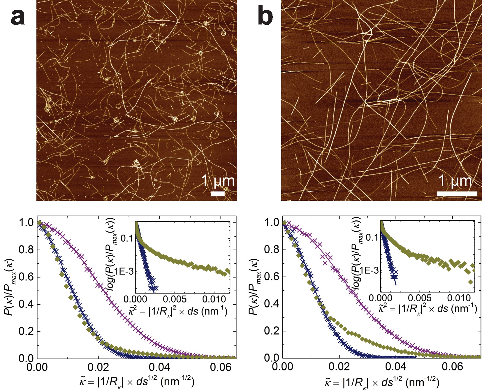
Figure 4: Fibrils exhibit a spontaneous curvature when adsorbed to a surface. Upper panel: zoomed in images of $\beta$-lactoglobulin fibrils (a) at the air-water interface after $t=10$ minutes of adsorption from a $c_{\text{init}}=0.001\%$ w/w fibril suspension and (b) deposited onto mica for $2$ minutes from the bulk with $c_{\text{init}}=0.1\%$ w/w. Lower panel: probability distributions of normalized absolute local curvatures $\kappa$ extracted from the full (a) $30\times 30$ $\mu\text{m}$ (see Appendix for full image) and (b) $5\times 5$ $\mu\text{m}$ images (green diamonds) with a $ds$ of $24$ and $9.8$ nm, respectively. The curvature distribution of simulated WLCs generated using all relevant parameters from the corresponding AFM image (see Methods) is shown as purple crosses and is successfully fitted with a Gaussian probability distribution function (purple line). Tracking these WLCs results in a change in the probability densities (blue crosses) but the values are still Gaussianly distributed (blue line). Plotting the normalized probabilities in logarithmic scale as a function of $\kappa^{2}$ clearly shows fat tails and thus the presence of spontaneous curvature only in real fibrils (Insets in the lower panel).

It has been argued that differences in $\kappa_{0}$ are to be expected depending on the strength of adsorption to the surface ³⁵ and on whether the polymer is in 3D or 2D ³⁶. To test this, we compare the curvature distributions from fibrils adsorbed to the air-water interface and transferred horizontally to mica (Fig. 4a) to fibrils deposited onto mica from a drop of the bulk solution (Fig. 4b). The modified Langmuir-Schaefer AFM sample preparation is a 2D to 2D transfer from a liquid onto a solid surface, which is much faster (milliseconds) than the slower (seconds) 3D to 2D equilibration obtained by depositing onto a solid substrate from bulk ³⁴. The bending probability of fibrils adsorbed from the bulk to mica, where no rings are observed, was also found to deviate from a typical Gaussian distribution (Fig. 4b). Fibrils hence bend as a result of their exposure to the inhomogeneous environment of solid-liquid, liquid-liquid, and gas-liquid interfaces, independently of how they initially adsorbed at these phase boundaries.

2.4 Average Fibril Thickness Determines Propensity to Bend

Figure 5: Fibril thickness affects probability of observing rings at the air-water interface. (a-d) Fraction of double- (solid bar) and triple-stranded fibrils (striped bar) in batches of fibrils formed from $\beta$-lactoglobulin obtained from three different suppliers. Data correspond to the ratio of the area under each of the two peaks to the total area of the average height per fibril distribution obtained on AFM samples of fibrils at the air-fibril solution interface with $c_{\text{init}}=0.001\%$ w/w. Rings are observed most frequently in batch 1 from source 1 (a), looped structures are found in fibrils from source 2 (b), and batch 2 from source 1 (c), whereas fibrils from source 3 do not form rings (d). The scale bar applies to all AFM images. (e) Probability distributions of normalized absolute local curvatures $\kappa$ for only double- (blue diamonds) and only triple-stranded fibrils (purple diamonds) for the sample shown in a and Fig. 4a. Less spontaneous curvature is found for thicker fibrils (inset). (f) Probability distributions of normalized absolute local curvatures $\kappa$ for the samples shown in a (green diamonds), b (blue diamonds), c (green stars) and d (purple diamonds). Samples with higher fractions of thicker fibrils have less pronounced fat tails in their normalized ${\cal P}(\kappa)$ distribution (inset).

As noted above, we predict a larger fibrillar diameter to imply a larger bending modulus, and hence a smaller likelihood of bending spontaneously (according to Eq.2.7). This was confirmed by studying fibrils from different batches of preparation, as well as from different suppliers. Fig. 5 shows ratios of double- to triple-stranded fibrils for $\beta$-lactoglobulin fibrils produced from native protein obtained from three different suppliers. Non-identical distributions can be expected due to different fibril processing conditions (sample volumes, shearing and stirring histories) between batches, and/or genetic variants between suppliers ³⁷. This then affects the individual filament thickness, and number of filaments per fibril, due to subtle differences in proteolysis. Thicker filaments, with larger bending moduli, should have much smaller spontaneous curvatures, and not be visibly curved if thick enough. Fig. 5 shows the distribution of number of strands per fibril, which is proportional to thickness, as determined from the AFM images. The batch with the highest number of rings (Fig. 1) contains the largest amount of double-stranded fibrils (Fig. 5a). By contrast, for batches of fibrils formed with the same protocol but from protein obtained from a different supplier, primarily three-stranded fibrils were found, which did not assemble into rings (Fig. 5d). Both a second batch of fibrils from the first source as well as a batch from a third supplier containing a more even mix of double- and triple-stranded fibrils yielded curved conformations (Fig. 5b and c). By separating the data used to calculate the normalized distribution of ${\cal P}(\kappa)$ presented in Fig. 4a into double- and triple-stranded fibrils (Fig. 5e), we confirm that the normalized ${\cal P}(\kappa)$ distribution of thick fibrils has a less pronounced fat tail and these fibrils thus bend less than their thinner counterparts. A similar trend is observed for the different batches in Fig. 5a-d, where a higher fraction of thicker fibrils in the sample results in less curved structures at the air-water interface and less spontaneous curvature (Fig. 5f).

3 Conclusions

We provide evidence from three different and independent experimental techniques for the presence of complex self-assembled amyloid fibril structures at air-water and oil-water interfaces. It has previously been reported that fibril ends are particularly reactive, as shown in the disruption of liposomes occurring preferentially at fibril ends ³⁸. Their enhanced fibrillation properties as compared to the rest of the fibrils ^{39, 40, 41, 42} in addition to possible capillary interactions ⁴³ may play a role in the observed tendency of fibrils to form almost-closed rings. The genesis of these rings and loops is explained by a spontaneous curvature arising from the interaction of polar, chiral and semiflexible fibrils with an interface. Because a spontaneous curvature but no ring formation was determined in fibrils at the solid mica-liquid interface, it can be concluded that a certain degree of mobility at the interface supports the assembly of fibrils into such geometries. This is in agreement with the fact that amyloid fibrils adsorbed onto a mica surface from bulk can asymptotically reach the expected $3/4$ exponent for a self-avoiding random walk in 2D ^{44, 45}. The ability of fibrils to form rings correlates with the average fibril height distribution, with loops only observed in systems where single- and double-stranded fibrils dominate. A shift in fibril height towards more triple-stranded populations reduces the number of high curvature counts and thus the amount of ring structures present. It is noteworthy, however, that a spontaneous curvature is expected also for thicker fibrils but at lower $\kappa$ because of their higher bending modulus, meaning that only thick fibrils which are long enough ($L\geq 2\pi/\kappa$) will be able to form full rings. These findings have consequences for the understanding of how fibrils deposit $in$ $vivo$, the morphology of plaques, biomechanical interactions of chiral filaments with surrounding tissues, and ultimately their effect on cells and organisms. A larger natural dynamic analogue in the form of the circular motion of polarly flagellated bacteria near solid surfaces has been described in the literature ⁴⁶ and together, these results could be seen as a new approach for the controlled design, fabrication or improvement of nanoswimmers and -robots.

4 Experimental

4.1 Fibril Formation

Amyloid $\beta$-lactoglobulin fibrils were prepared according to the protocol of Jung et al. ¹⁵. The native, freeze-dried protein was obtained from three different sources: Davisco, Sigma, and TU Munich ⁴⁷. A $2$% w/w solution of purified and dialyzed $\beta$-lactoglobulin was stirred during 5 hours at 90 ^∘C and $p\text{H}$ $2$. The resultant fibrils were then dialyzed against $p\text{H}$ $2$ MilliQ water for 5 to 7 days to remove unconverted proteinaceous material. There is, however, evidence that even after complete removal of non-fibrillar material, the system will go back to an equilibrium point where both fibrils and ”free” peptides are present. This has been proposed for the case of A$\beta_{1-40}$ and SH3 domain fibrils ^{48, 40} and recently for $\beta$-lactoglobulin ^{17, 49}. Another pathway for the accumulation of peptides may be the disaggregation of fibrils upon adsorption to the air-water interface.

4.2 Atomic Force Microscopy

Sample preparation and atomic force microscopy (AFM) were performed as described previously ¹⁷. All samples contained no added salt. For the modified Langmuir-Schaefer technique, a $2$ $\mu$L aliquot of a fibril solution of desired concentration $c_{\text{init}}$ was carefully pipetted into a small glass vial and left to stand for time $t$. For a given $c_{\text{init}}$ the interfacial fibril density increases with $t$ as more fibrils adsorb to the interface. A freshly cleaved mica sheet glued to a metal support was lowered towards the liquid surface horizontally and retracted again immediately after a brief contact. The mica was then dipped into ethanol ($\geq 99.8$% v/v) to remove any unadsorbed bulk material before drying the sample under a weak clean air flow. Alternatively, images of fibrils in the bulk were collected by pipetting $20$ $\mu$L of the sample onto a freshly cleaved mica. After two minutes, the mica was gently rinsed with MilliQ water and dried with pressurized air. Sample scanning in air was performed on a Nanoscope VIII Multimode Scanning Probe Microscope (Veeco Instruments) in tapping mode.

4.3 Passive Probe Particle Tracking

A volume of $15$ $\mu$L of a $c_{\text{init}}=0.001\%$ w/w fibril sample seeded with $0.075\%$ w/v fluorescein isothiocyanate labelled, positively charged silica tracer particles of diameter $\approx{774}$ nm, was pipetted into an epoxy resin well on a thoroughly cleaned and plasma-treated glass coverslide. Medium chain triglycerides were poured on top so as to create a flat oil-water interface. The motion of tracers trapped at this interface was then recorded on an inverted microscope (Leica DM16000B) equipped with a $63\times 1.4$ NA oil HCX PlanApo DIC objective for up to $700$ frames at a rate of $0.374$ s. Images were analysed with standard as well as custom-written software in IDL (ITT Visual Information Solutions) ^{50, 16, 17}

4.4 Cryogenic Scanning Electron Microscopy

Samples for freeze-fracture cryogenic Scanning Electron Microscopy (FreSCa cryo-SEM ⁵¹) were prepared by creating a flat medium chain triglycerides (MCT)-fibril solution interface in clean, small copper holders. The fibril solution contained the same concentration of fluorescent tracer particle as in passive probe particle tracking experiments and were added here for easier location of the interface during imaging. The samples were then frozen at a cooling rate of $30000$ Ks^-1 in a liquid propane jet freezer (Bal-Tec/Leica JFD 030) and fractured under high vacuum at $-140$ ^∘C (Bal-Tec/Leica BAF060). After partial freeze-drying at $-110$ ^∘C for 3 minutes to remove ice crystals and condensed water from the sample surfaces, they were coated with a $2$-nm thin layer of tungsten at $-120$ ^∘C. All samples were transferred to the precooled cryo-SEM (Zeiss Gemini 1530) under high vacuum ($\lesssim{5\times 10^{-7}}$ mbar) with an air-lock shuttle. Imaging was performed at $-120$ ^∘C with a secondary electron detector.

4.5 Local Curvature Determination

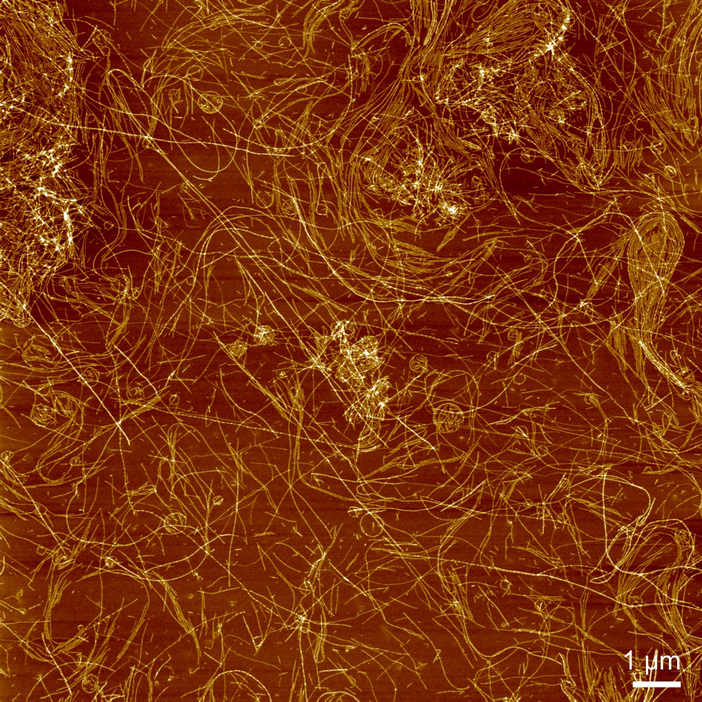
Figure S7: AFM image of fibrils at the air-water interface after $t$=10 minutes adsorption time from a $c_{\text{init}}\approx{0.008}$% w/w fibril suspension. Rings coexist with nematic fibril domains.

A home-built fibril tracking routine based on open active contours ³⁴ was used to extract the fibrils’ $xy$ coordinates from AFM images with a tracking step length $\Delta s\approx 1$ pixel between two subsequent points along a tracked fibril. Any fibrils involved in ring formation as well as those deposited from the subphase (for example the bright ones running from top left to bottom right of the image in Fig. S7) were discarded from the analysis. The absolute local curvature $\kappa=|1/R_{\kappa}|$ with $R_{\kappa}$ being the radius of curvature between two vectors v${}_{\textbf{1}}$ and v${}_{\textbf{2}}$ of equal length along the fibril contour with a distance $ds$ between them, was calculated for all fibril segment pairs in the image of interest. The curvature is given by $1/R_{\kappa}=($v${}_{\textbf{2}}(s+ds)-$v${}_{\textbf{1}}(f))/|$v$|ds$, where we chose $ds=2\Delta s$. For a fibril penalized by only a bending energy, the probability of a curved segment is given by

$${\cal P}(\kappa)={\cal N}e^{-\tfrac{1}{2}\ell_{p}\kappa^{2}ds},$$ (4.1)

where ${\cal N}$ is a normalization factor, and $\ell_{p}=B/k_{\scriptscriptstyle B}T$ is the persisence length ². The distribution depends on the segment length $ds$ chosen for the calculation of bending. Of course, the intrinsic persistence length is a material property and cannot depend on this discretization. Hence, the distribution of the quantity $\tilde{\kappa}=\kappa\sqrt{ds}$ is independent of the image resolution, and was used to parametrize the distribution of curvatures.

Images of WLCs were generated using the following parameters obtained from real AFM fibril images:

1. the mean and variance of the length distribution,

2. the average fibril radius,

3. the number of fibrils per image,

4. $\ell_{p}$ determined from the fit of the average 2D mean squared end-to-end distance

   $$\langle R^{2}_{2D}\rangle=4L_{c}\ell_{p}\left[1-2\frac{\ell_{p}}{L_{c}}\left(1-e^{-L_{c}/2\ell_{p}}\right)\right],$$ (4.2)

   where $L_{c}$ is the internal contour length,

5. fibril tracking step $\Delta s$,

6. and discretization $ds$.

The WLC coordinates from which the artifical images were created, were used as such for the calculation of ${\cal P}(\kappa)$. Additionally, the generated chains were tracked with the same algorithm used for real AFM images to illustrate the change in ${\cal P}(\kappa)$ due to resolution limits in the imaging and the apparently lower but purely Gaussian curvature distribution in tracked WLCs compared to untracked WLCs.

To calculate the curvature distribution for either double- or triple-stranded fibrils, the tracked fibril data set was separated into two based on a cut-off height obtained from the average fibril height histogram.

Support by the Electron Microscopy of ETH Zurich (EMEZ) is acknowledged and the authors thank A. Schofield for the silica tracers. L. Böni is thanked for his help with figure design. The authors acknowledge financial support for S.J. from ETH Zurich (ETHIIRA TH 32-1), I.U. from SNF (2-77002-11), P.D.O. from an SNSF visiting fellowship (IZK072_141955), and L.I. from SNSF grants PP00P2_144646/1 and PZ00P2_142532/1.

Appendix A Appendix – Supplementary Information

A.1 Persistence of Rings in the Presence of Nematic Domains

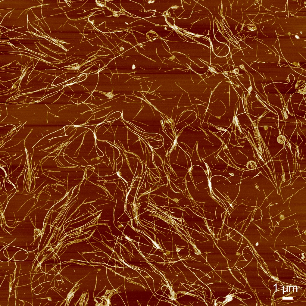
Figure S6: AFM image of fibrils at the air-water interface after $t$=60 minutes adsorption time from a $c_{\text{init}}=0.001$% w/w fibril suspension.

Rings can be observed even at high interfacial fibril densities, where nematic domains cover most of the observed area as shown in Fig. S6 and S7. At this point, the rings are usually composed of many fibrils or are completely filled by short fibrils. It is worth noting, however, that some regions on the same sample can be void of rings. There is a population of fibrils in all four batches investigated that is not consistent with the height and pitch distributions observed in ¹. These fibrils are very tightly wound with a half-pitch length around $40$ nm and a maximum height between $4$ and $7$ nm and can also be seen to partake in ring formation.

A.2 Spontaneous Bending of a Polar Twisted Ribbon at an Interface

A.2.1 Surface Interaction

Most particles, including proteins, adsorb to a hydrophobic-hydrophilic interface in order to reduce the nascent hydrophobic surface tension ². In addition to this, a protein will interact specifically with the two media according to the nature of the amino acids. Such interactions are both short-range (charge, hydrophobic effect, steric shapes) and long-range (dispersion interactions) ³. Long range interactions depend weakly on the nature of the surface, as they typically include the bulk of the two interface materials and the entire protein. However, the short range surface interactions depend critically on the details of the surface of the protein. The inhomogeneous surface of a protein results in a local moment or torque applied by the fluid at each point on the surface. For a helical protein immersed in a homogeneous fluid, this local torque will sum to zero across the entire surface of the protein. However, for a protein in an inhomogeneous environment, such as one confined to an interface, will experience a non-zero total torque $\Gamma$. This can induce a spontaneous curvature or twist depending on both the direction of $\Gamma$ and the strength of the intrinsic bend and twist moduli.

The net torque on the protein due to its environment can be separated into contributions from short range and long range forces:

$${\Gamma} =\int_{V}\!d^{3}r\,\mathbf{r}\times\mathbf{f}_{LR}(\mathbf{r})+\Delta\int_{S}d^{2}r\,\mathbf{r}\times\mathbf{f}_{SR}(\mathbf{r},z)\,,$$ (A.1)

$$\mathbf{f}(\mathbf{r}) =-\int_{\textrm{env}}d^{3}r^{\prime}\,\frac{\partial{\cal U}\left(\mathbf{r}-\mathbf{r}^{\prime}\right)}{\partial(\mathbf{r}-\mathbf{r}^{\prime})},$$ (A.2)

where the energy density ${\cal U}(\mathbf{r}-\mathbf{r}^{\prime})$ of interaction (energy per volume squared) between material in the environment at $\mathbf{r}^{\prime}$ and in the protein at $\mathbf{r}$ can be separated into long range (e.g. dispersion or Coulomb) and short-range (e.g. hydrophobic or steric) interactions. Here, $\Delta$ is the interaction depth within the protein (of order an amino acid in size), and the forces are obtained by integrating over points $\mathbf{r}^{\prime}$ in the environment external to the protein. Although the net torque will generally depend on the entire shape and volume of the protein (because of long range dispersion and Coulomb interactions), we will illustrate the example where the effects of long range forces are negligible compared to those of the short range interactions. For example, an unbalanced torque that leads to a bend in the plane of the interface will not perturb the long range energy of interaction appreciably, since there will be neligible response perpendicular to the interface.

In the case of short range interactions, we can approximate the integral over the environment as $\int_{\textrm{env}}d^{3}r^{\prime}\simeq a\int dz^{\prime}$, where the coordinate $z^{\prime}$ is along the surface normal and $a$ is the lateral area of the short interaction. By integrating the short range potential and using the reference ${\cal U}(z=\infty)=0$, we can write the torque exerted on the surface as

$${\Gamma} =a\Delta\int_{S}d^{2}r\,(\mathbf{r}\times\mathbf{\hat{{n}}})\,{\cal U}(\mathbf{r}),$$ (A.3)

$$\equiv\int_{S}d^{2}r\,(\mathbf{r}\times\mathbf{\hat{{n}}})\,\left[\bar{\gamma}+\delta\gamma\left(\mathbf{r}\right)\right],$$ (A.4)

The quantity $(a\Delta){\cal U}(\mathbf{r})\equiv\bar{\gamma}+\delta\gamma(\mathbf{r})$ is the surface energy density of interaction introduced in Eq. [3] of the main text.

Fluid-fluid interface – At fluid-fluid interfaces an adsorbed fibril will be surrounded by both fluids, according to the (inhomogeneous) degree of wettability of the fibril on the two fluids. This inhomogeneous environment leads to a net uncompensated moment when averaged over the inhomogenous solvent environment around the fibril. Although this applies to the problem at hand, we will take the a pragmatic approach and illustrate the method for the simpler example of a fluid-solid interface with short-range interactions.

Fluid-solid interface – Consider a fibril adsorbed to a fluid-solid interface. Material within a short range $\Delta$, set by Coulomb screening, shapes of asperities, or hydrophobic effects, will interact with the solid substrate on a strip. For short range interactions a surface interaction that is symmetric from head to tail (a non-polar interaction) will lead to zero applied total torque, as the local torque will sum to zero, as in a homogeneous environment. However, a non-symmetric interaction will lead to uncompensated torques, or bending moments, all along the length of the adsorbed fibril.

A.2.2 Twisted Ribbon of Fixed Radius

To make progress, we approximate the fibril of length $L$ as a twisted ribbon with wavelength $\lambda$, which makes contact every half wavelength with a solid surface on the exposed edges at the ribbon radius $R$ (Figures S10, S11). The wavelength is related to the helical angle $\theta_{p}$ by

$$\cos{\theta_{p}} =\frac{qR}{\sqrt{1+(qR)^{2}}} \sin{\theta_{p}} =\frac{1}{\sqrt{1+(qR)^{2}}},$$ (A.5)

where $q=2\pi/\lambda$. The centerline of the undeformed fibril defines a tangent vector $\mathbf{\hat{{t}}}_{0}$, which upon bending becomes $\mathbf{\hat{{t}}}(s)$, with local curvature $\kappa=|d\mathbf{\hat{{t}}}/ds|\equiv|\dot{\hat{\textbf{t}}}|$. Equivalently, we can parametrize the curvature in terms of the vector angular rotation of the tangent vector, defined by $\dot{\boldsymbol{\Theta}}=\mathbf{\hat{{t}}}\times\dot{\hat{\textbf{t}}}$.

Rather than work in terms of torques exerted across the body, we will calculate the surface energy of the adsorbed fibril as a function of the fibril shape. Minimizing this energy with respect to in-plane bending will lead to an induced spontaneous curvature, which is equivalent to finding an uncompensated torque for a straight fibril.

For a small interaction range, $\Delta\ll R$, the interaction between the surface and the twisted ribbon can be approximated by the surface energy of series of strips of thickness $\omega=2\sqrt{2R\Delta-\Delta^{2}}\simeq\sqrt{8R\Delta}$ (Fig. S10). The ribbon-surface energy is given by

$$G_{\textrm{surf}} =\sum_{j=1}^{2L/\lambda}\int_{S_{j}}\left[\bar{\gamma}+\delta\gamma(\mathbf{r})\right]d^{2}r$$ (A.6)

$$\equiv\sum_{j=1}^{2L/\lambda}G_{\textrm{polar},j},$$ (A.7)

where $S_{j}$ is the surface area of the $j$th interaction strip, the average surface energy $\bar{\gamma}$ represents the absorption properties of the ribbon, and $\delta\gamma$ captures the polar nature of the interaction. There are $2L/\lambda$ distinct interaction strips. We assume that the strip has an anisotropic interaction potential that is polar along the direction $\mathbf{\hat{{u}}}$ within the strip, and assume the simple form

$$\delta\gamma(\mathbf{r}) =\varepsilon\,\mathbf{r}\cdot\mathbf{\hat{{u}}}$$ (A.8a)

$$=\varepsilon\left(x\cos\Phi+y\sin\Phi\right),$$ (A.8b)

where $\mathbf{\hat{{u}}}$ is at an angle $\Phi$ with respect to the tangent vector $\mathbf{\hat{{t}}}$.In the limit of $R\gg\Delta$ the strips can be approximated as flat, taking $\mathbf{r}$ as a two-dimensional vector in the plane of the surface. For short range interactions these flat strips constitute the primary interaction between the surface and the twisted ribbon.

Amyloid fibrils are composed of protofilaments, which in turn comprise layers of aligned beta sheets that are twisted about their central axis. A given fibril contains a number of protofilaments that form a ribbon, which we approximate as shown in Figure S11(A). The ribbon diameter $D$ is given by the number of protofilaments in the fibrils, while the ribbon thickness $d$ is determined by the diameter of an individual protofilament. The ribbon length $L$ is determined by the total number of aligned beta strands.

For an undeformed fibril the interaction strip is a parallelogram tilted at an angle $\theta_{p}$ determined by the pitch of the ribbon, and with lengths determined by the thickness $d$ of the ribbon (the perpendicular distance between the edges) and the strip thickness $\omega$, as shown in Figure S11(B). Two sides of length $\ell=d/\sin\theta_{p}$ are parallel to the tangent vector $\mathbf{\hat{{t}}}_{0}$, while the other two sides have length $\omega/\cos\theta_{p}$.

When the ribbon is bent the ribbon thickness $d$ is fixed due to the fixed radius, but it curves to follow the deformed tangent vector $\mathbf{\hat{{t}}}$. Given that we are in the small bend regime, we approximate these sides as straight, but tilted additionally by $\bar{\phi}=\tfrac{1}{2}(\phi_{R}+\phi_{L})$ according to the average tilt of the interaction strip (Figure S11(C)). Here $\phi_{L}$ and $\phi_{R}$ represent the additional tilts on the left and right hand sides of the interaction strip.

When the strip is bent downwards the top of the interaction strip is under tension whereas the bottom of the strip is under compression. Although the center of the strip is not under tension or compression, bend-stretch coupling terms may cause the ribbon to stretch or compress, leading to a new strip length $\ell^{\prime}=d/\sin(\theta_{p}-\bar{\phi})$. This change in length contributes to the bend-stretch coupling, which is not of interest here.

Initially, the polarity vector $\mathbf{\hat{{u}}}_{0}$ is at an angle $\Phi$ with respect to the tangent vector $\mathbf{\hat{{t}}}_{0}$. When the twisted ribbon is bent, then to first order the all vectors in the interaction strip rotate with the average rotation $\bar{\phi}$ of a particular segment; this includes both the polarity vector and the local tangent vector. However, the stretching and compression on either side of the bend cause the polarity vector to deflect non-affinely aross the strip; e.g the tilt of the polarity vector should vary smoothly between $\phi_{L}$ and $\phi_{R}$, when moving from left to right across the strip. For simplicity we will take the polarity vector to be tilted by $\bar{\phi}$ everywhere on the interaction strip. With this notation, the polar surface potential becomes

$$\left.\delta\gamma(\mathbf{r})\right|_{\textrm{bent}}=\varepsilon\left[x\cos(\Phi-\bar{\phi})+y\sin(\Phi-\bar{\phi})\right].$$ (A.9)

A.2.3 Polar Free Energy

The polar energy across a single interaction strip, or equivalently the energy per helical repeat, is then given by

$$G_{\textrm{polar}} =\varepsilon\int^{\tfrac{1}{2}\omega}_{-\tfrac{1}{2}\omega}\,dy\,\int^{f_{R}(y)}_{f_{L}(y)}\,dx\left[x\cos\left(\Phi-\bar{\phi}\right)+y\sin\left(\Phi-\bar{\phi}\right)\right],$$ (A.10)

$$f_{L}(y) =y\cot[\theta_{p}+\tfrac{1}{2}(\phi_{R}-\phi_{L})]-\tfrac{1}{2}\ell$$ (A.11)

$$f_{R}(y) =y\cot[\theta_{p}-\tfrac{1}{2}(\phi_{R}-\phi_{L})]+\tfrac{1}{2}\ell\,,$$ (A.12)

and $\ell$ is the length of center of the interaction strip parallel to $\mathbf{\hat{{t}}}_{0}$. This evaluates to

$$G_{\textrm{polar}}= \frac{\varepsilon\omega^{3}}{12}\left[\cot\left(\theta_{p}-\tfrac{1}{2}\Theta\right)-\cot\left(\theta_{p}+\tfrac{1}{2}\Theta\right)\right]\left\{{\sin}\left(\Phi-\bar{\phi}\right)\right.$$

$$\left.\tfrac{1}{2}{{\cos}\left(\Phi-\bar{\phi}\right)}\left[\cot\left(\theta_{p}-\tfrac{1}{2}\Theta\right)+\cot\left(\theta_{p}+\tfrac{1}{2}\Theta\right)\right]\right\},$$ (A.13)

where ${\Theta=\phi_{R}-\phi_{L}}$ is the angular deflection associated with the bend. The energy of deformation vanishes for zero bend $\Theta=0$. A positive bend $\Theta>0$ corresponds to a right hand bend, when travelling parallel to the chosen direction fo the tangent vector.

Our goal is to study the lowest order effects of the surface, which induce a spontaneous curvature signified by the term linear in bend $\Theta$ that arises from the small $\Theta$ approximation to $G_{\textrm{polar}}$. The average tilt $\bar{\phi}$ can be related, geometrically, to a combination of twist and stretch, which leads to surface-induced bend-twist and bend-stretch couplings. Thus, we will expand Eq. A.13 to first order in $\Theta$, and set $\bar{\phi}=0$ because we are not interested in higher order bend-twist or bend-stretch couplings (the effects of these would only be visible upon observing changes in total fibril length, or in local chirality). To lowest order in the deflection we find

$$G_{\textrm{polar}} =\frac{\varepsilon\omega^{3}}{12\sin^{2}\theta_{p}}(\cos\Phi\,{\cot\theta_{p}}+\sin\Phi)\,\Theta+\ldots\,$$ (A.14)

$$\simeq\frac{\varepsilon\omega^{3}\ell}{12\sin^{2}\theta_{p}}(\cos\Phi\,{\cot\theta_{p}}+\sin\Phi)\,\frac{d\Theta}{ds}.$$ (A.15)

In performing this expansion we have assumed that the polar direction $\mathbf{\hat{{u}}}$ (or $\Phi$) rotates affinely with the tangent; deviations from this will lead to higher order couplings $\Theta\,\delta\Phi$. Hence, the contribution to the bending energy of the entire fibril is

$$G_{\textrm{surf}} =\sum_{j=1}^{2L/\lambda}G_{\textrm{polar},j}$$ (A.16)

$$=\int_{0}^{L}\frac{2\,ds}{\lambda}\frac{\varepsilon\omega^{3}\ell}{12\sin^{2}\theta_{p}}(\cos\Phi\,{\cot\theta_{p}}+\sin\Phi)\,\,\frac{d\Theta}{ds},$$ (A.17)

where we have assumed that the bend is smooth between contacts, and converted the sum to an integral via $\sum_{j}\rightarrow\int ds/\lambda$.

The polar moment is given by

$$\mathbf{P} =\frac{2}{\lambda}\int_{S}\,\mathbf{r}\,\delta\gamma(\mathbf{r})\,\,d^{2}r,$$ (A.18)

$$=\frac{2\varepsilon}{\lambda}\int_{S}\,\mathbf{r}\,(\mathbf{r}\cdot\mathbf{\hat{{u}}})\,\,d^{2}r,$$ (A.19)

$$=\frac{\varepsilon}{\lambda}\frac{\partial}{\partial\mathbf{\hat{{u}}}}\int^{\frac{\omega}{2}}_{-\frac{\omega}{2}}dy\int^{y\cot\theta_{p}+\tfrac{\ell}{2}}_{y\cot\theta_{p}-\tfrac{\ell}{2}}\left[x\cos\Phi+y\sin\Phi\right]^{2}\,dx$$ (A.20)

$$=\frac{\varepsilon\omega^{3}\ell}{6\lambda}\left\{\left[\cos\Phi\left(\cot^{2}\theta_{p}+\left(\frac{\ell}{\omega}\right)^{2}\right)+\sin\Phi\cot\theta_{p}\right]\mathbf{\hat{{t}}}+\left(\sin\Phi+\cos\Phi\cot\theta_{p}\right)\mathbf{\hat{{n}}}\times\mathbf{\hat{{t}}}\right\}.$$ (A.21)

One component of $\mathbf{P}$ is parallel to the fibril direction $\mathbf{\hat{{t}}}$, while the other direction is perpendicular to $\mathbf{\hat{{t}}}$ and in the plane specified by normal vector $\mathbf{\hat{{n}}}$. Note that $\{\mathbf{\hat{{t}}},\mathbf{\hat{{n}}}\times\mathbf{\hat{{t}}},\mathbf{\hat{{n}}}\}$ form an orthonormal basis. Hence,

$$\mathbf{P}=P_{\parallel}\mathbf{t}+P_{\perp}\mathbf{\hat{{n}}}\times\mathbf{\hat{{t}}},$$ (A.22)

where

$$P_{\parallel} =\frac{\varepsilon\omega^{3}\ell}{6\lambda}\left[\cos\Phi\left(\cot^{2}\theta_{p}+\left(\frac{\ell}{\omega}\right)^{2}\right)+\sin\Phi\cot\theta_{p}\right]$$ (A.23a)

$$P_{\perp} =\frac{\varepsilon\omega^{3}\ell}{6\lambda}\left(\sin\Phi+\cos\Phi\cot\theta_{p}\right).$$ (A.23b)

Comparing the definition of $\mathbf{P}$ with the free energy $G_{\textrm{surf}}$, we can rewrite the surface energy as

$$G_{\textrm{surf}} =\frac{1}{\sin^{2}\theta_{p}}\int_{0}^{L}ds\,{P_{\perp}}\,\frac{d\Theta}{ds}.$$ (A.24)

In vector form, the angular rotation is given by $\dot{\boldsymbol{\Theta}}=-\mathbf{\hat{{n}}}\frac{d\Theta}{ds}$ (Fig. S11), while the component $P_{\perp}$ can be extracted via $P_{\perp}=\mathbf{\hat{{n}}}\cdot\mathbf{\hat{{t}}}\times\mathbf{P}$. Thus, the free energy becomes

$$G_{\textrm{surf}} =-\frac{1}{\sin^{2}\theta_{p}}\int_{0}^{L}ds\,\dot{\boldsymbol{\Theta}}\cdot\mathbf{\hat{{t}}}\times\mathbf{P},$$ (A.25)

which corresponds to the free energy of Equations 5-6 in the main text, with $A=1/\sin^{2}\theta_{p}$.

A.2.4 Induced Curvature

The total bending free energy is given by the sum of the standard bending energy and the coupling to the surface:

$$G_{bend} =\int ds\left[\frac{1}{2}B\dot{\boldsymbol{\Theta}}^{2}-\frac{1}{\sin^{2}\theta_{p}}\dot{\boldsymbol{\Theta}}\cdot\mathbf{\hat{{t}}}\times\mathbf{P}\right]$$ (A.26)

$$=\int ds\left[\frac{1}{2}B\kappa^{2}-\frac{\varepsilon\omega^{3}\ell}{6\lambda\sin^{2}\theta_{p}}(\cos\Phi\,{\cot\theta_{p}}+\sin\Phi)\kappa\right],$$ (A.27)

where the (signed) curvature is defined by $\dot{\Theta}=\kappa\mathbf{\hat{{n}}}$. The bending modulus generally includes contributions from the surface, which can be calculated based on the formalism here. However, since our intent is to demonstrate the significance of the induced curvature, we do not consider such perturbations. Moreover, the main contribution to bending is usually from internal degrees of freedom that are only weakly influenced by the surface. An exception occurs for highly charged filaments. In such cases the reduction in the dielectric constant and lack of screening near a hydrophobic surface will increase the electrostatic contribution to $B$.

This bend energy is minimized by the following spontaneous curvature $\kappa_{0}$:

$$\kappa_{0} =\frac{\varepsilon\omega^{3}\ell}{6\lambda\sin^{2}\theta_{p}\,B}(\cos\Phi\,{\cot\theta_{p}}+\sin\Phi)$$ (A.28)

$$=\frac{\varepsilon\omega^{3}\ell}{\lambda\sin^{2}\theta_{p}\,B}\alpha(\theta_{p},\Phi),$$ (A.29)

where $\alpha(\theta_{p},\Phi)\equiv(\cos\Phi\,{\cot\theta_{p}}+\sin\Phi)/6$.

The sign of the induced curvature can be understood as follows. Consider $\varepsilon>0$, a helix with an opening angle of $\theta_{p}=\pi/4$, and a polarization direction specified by $\Phi=\pi/6$ (roughly as in Figs. S10, S11). In this case there is a higher energy for exposing the upper right part of the parallelogram in Fig. S11 to the surface. Hence the preferred bending direction should be ‘up’ in Fig. S10 (rather than the downward shown), to allow the relatively less of the costly part of the surface interaction to attain more contact with the surface. This corresponds to a positive bend around $\mathbf{\hat{{n}}}$, given by $\dot{\boldsymbol{\Theta}}=\kappa_{0}\mathbf{\hat{{n}}}$ with $\kappa_{0}>0$ and matches the prediction in Eq. (A.28).

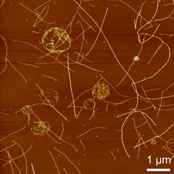
Figure S8: AFM image of fibrils at the air-water interface after $t$=60 minutes adsorption time from a $c_{\text{init}}=0.001$% w/w fibril suspension. Rings are often composed of many short fibrils.

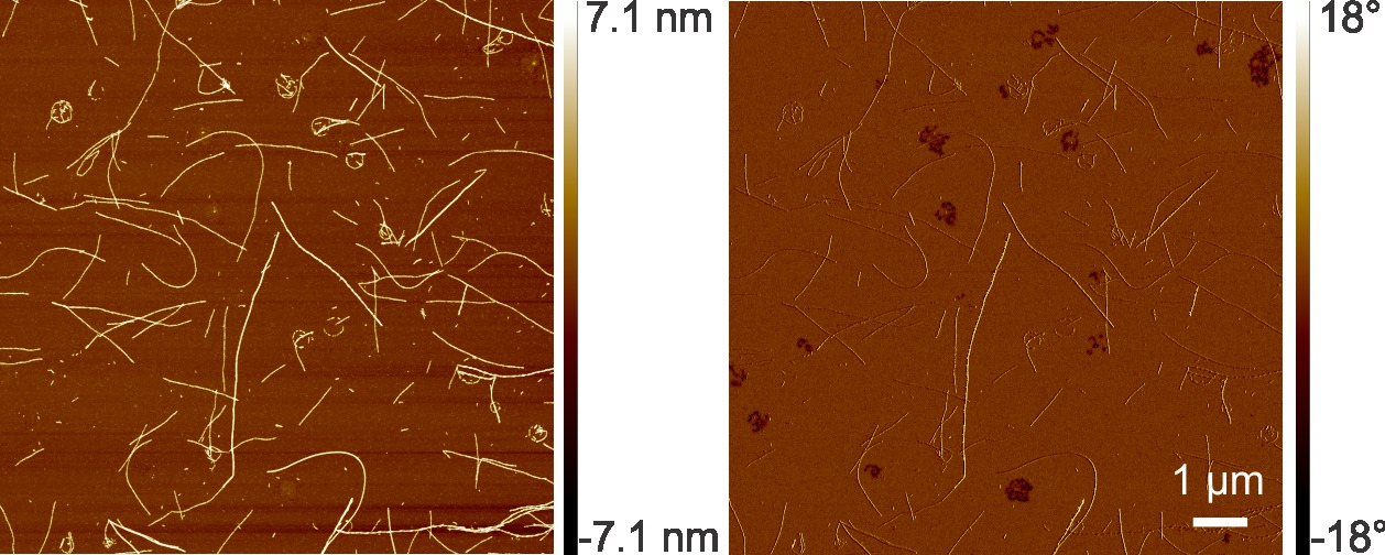
Figure S9: AFM height and phase images of fibrils at the air-water interface immediately after sample preparation of a $c_{\text{init}}=0.001$% w/w fibril suspension. The scale bar applies to both images. Distortions in the background peptide layer are readily visible in the phase image but are rarely spherical and do not coincide spatially with fibril rings.

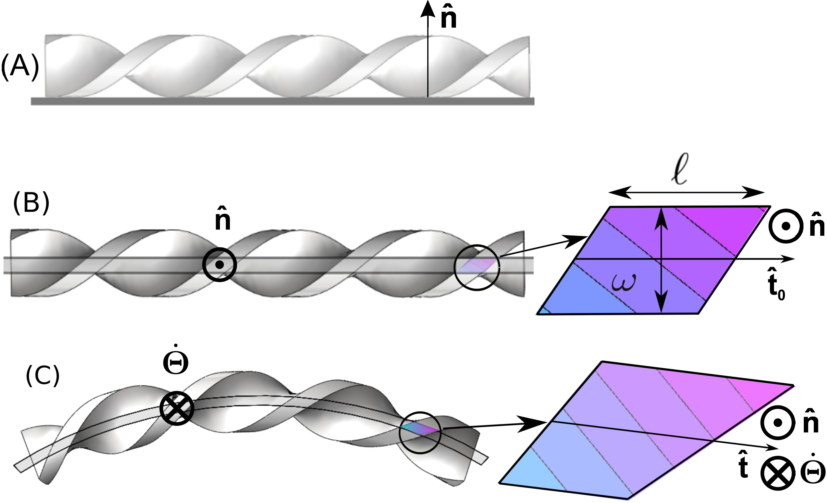
Figure S10: (A) Helical fibril against a surface. (B) The contact area, or interaction strip, is a parallelogram that deforms asymmetrically (C) when the fibril is bent. This leads to an excess contact area by one ‘charge’ of the polar interaction, leading to a preference for one sign of bend and thus a spontaneous curvature. A positive red ‘charge’ and a negative ‘blue’ charge corresponds to a polarization potential $\delta\gamma=\varepsilon(\cos\pi/6+y\sin\pi/6)$, with $\varepsilon>0$. In this case the bend shown in (C) costs energy, and the preferred spontaneous curvature instead correponds to a bend $\frac{d\boldsymbol{\Theta}}{ds}=\dot{\boldsymbol{\Theta}}=\mathbf{\hat{{t}}}\times\dot{\hat{\bf{t}}}$ which is parallel to $\mathbf{\hat{{n}}}$.

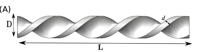
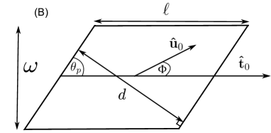
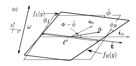
Figure S11: (A) Geometry of twisted ribbon. Initial (B) and deformed (C) interaction strips, obtained by bending the fibril. The undeformed strip is shown in grey under the deformed strip. The bend causes a tilt in the two sides (right and left) depending on the change in the tangent vector across the strip, while the top and bottom sides remain parallel to each other, but rotate with respect to the undeformed strip by $\bar{\phi}=\tfrac{1}{2}(\phi_{L}+\phi_{R})$, which describes the average tilt of the individual strip.

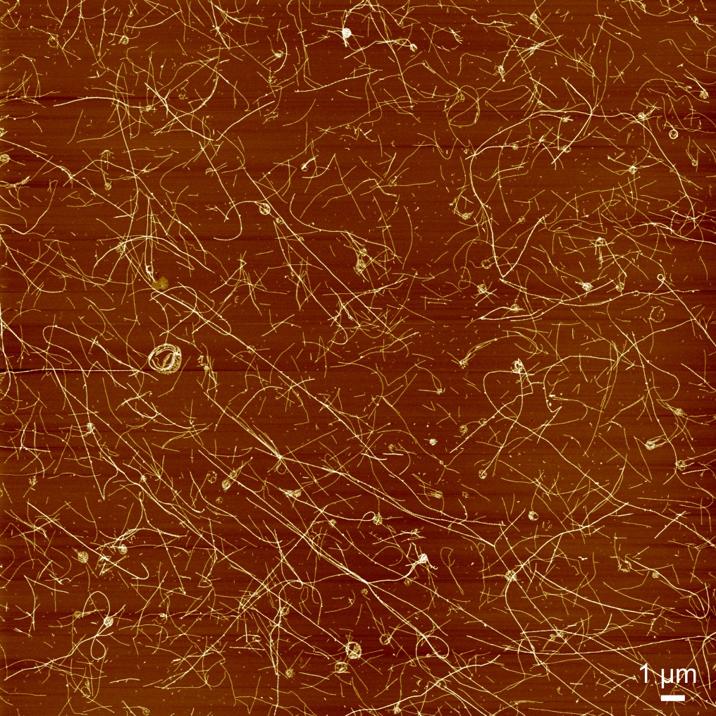
Figure S12: Whole AFM image used for the curvature distribution analysis showing fibrils at the air-water interface after $t$=10 minutes adsorption time from a $c_{\text{init}}=0.001$% w/w fibril suspension.

References

- 1 deGennes, P.-G. Scaling Concepts in Polymer Physics Cornell University Press: Ithaca, 1979.
- 2 Doi, M.; Edwards, S. F. The Theory of Polymer Dynamics Clarendon Press: Oxford, 1988.
- 3 Pereira, G. G. Charged, Semi-Flexible Polymers under Incompatible Solvent Conditions. Curr. Appl. Phys. 2008, 8, 347–350.
- 4 Cohen, A. E.; Mahadevan, L. Kinks, Rings, and Rackets in Filamentous Structures. Proc. Natl. Acad. Sci. USA 2003, 100, 12141–12146.
- 5 Hatters, D. M.; MacPhee, C. E.; Lawrence, L. J.; Sawyer, W. H.; Howlett, G. J. Human Apolipoprotein C-II Forms Twisted Amyloid Ribbons and Closed Loops. Biochemistry 2000, 39, 8276–8283.
- 6 Mustata, G.-M.; Shekhawat, G. S.; Lambert, M. P.; Viola, K. L.; Velasco, P. T.; Klein, W. L.; Dravid, V. P. Insights into the Mechanism of Alzheimer’s -Amyloid Aggregation as a Function of Concentration by Using Atomic Force Microscopy. Appl. Phys. Lett. 2012, 100, 133704–133704-4.
- 7 Paez, A.; Tarazona, P.; Mateos-Gil, P.; Vélez, M. Self-Organization of Curved Living Polymers: FtsZ Protein Filaments. Soft Matter 2009, 5, 2625–2637.
- 8 Tang, J. X.; Käs, J. A.; Shah, J. V.; Janmey, P. A. Counterion-Induced Actin Ring Formation. Eur. Biophys. J. 2001, 30, 477–484.
- 9 Kabir, A. M. R.; Wada, S.; Inoue, D; Tamura, Y.; Kajihara, T.; Mayama, H.; Sada, K.; Kakugo, A.; Gong, J. P. Formation of Ring-Shaped Assembly of Microtubules with a Narrow Size Distribution at an AirBuffer Interface. Soft Matter 2012, 8, 10863–10867.
- 10 Sumino, Y.; Nagai, K. H.; Shitaka, Y.; Tanaka, D.; Yoshikawa, K.; Chaté, H.; Oiwa, K. Large-Scale Vortex Lattice Emerging from Collectively Moving Microtubules. Nature 2012, 483, 448–452.
- 11 Jansen, R.; Grudzielanek, S.; Dzwolak, W.; Winter, R. High Pressure Promotes Circularly Shaped Insulin Amyloid. J. Mol. Biol. 2004, 338, 203–206.
- 12 Dobson, C. The Structural Basis of Protein Folding and Its Links with Human Disease. Phil. Trans. R. Soc. Lond. B 2001, 356, 133–145.
- 13 Eichner, T.; Radford, S. E. A Diversity of Assembly Mechanisms of a Generic Amyloid Fold. Mol. Cell 2011, 43, 8–18.
- 14 Adamcik, J.; Jung, J.-M.; Flakowski, J.; De Los Rios, P.; Dietler, G.; Mezzenga, R. Understanding Amyloid Aggregation by Statistical Analysis of Atomic Force Microscopy Images. Nature Nanotech. 2010, 5, 423–428.
- 15 Jung, J.-M.; Mezzenga, R. Liquid Crystalline Phase Behavior of Protein Fibers in Water: Experiments versus Theory. Langmuir 2010, 26, 504–514.
- 16 Isa, L.; Jung, J.-M.; Mezzenga, R. Unravelling Adsorption and Alignment of Amyloid Fibrils at Interfaces by Probe Particle Tracking. Soft Matter 2011, 7, 8127–8134.
- 17 Jordens, S.; Isa, L.; Usov, I.; Mezzenga, R. Non-Equilibrium Nature of Two-Dimensional Isotropic and Nematic Coexistence in Amyloid Fibrils at Liquid Interfaces. Nat. Commun. 2013, 4, 1917–1917-8.
- 18 Dobson, C. M. Protein Folding and Misfolding. Nature 2003, 426, 884–890.
- 19 Mankar, S.; Anoop, A.; Sen, S.; Maji, S. K. Nanomaterials: Amyloids Reflect Their Brighter Side. Nano Rev. 2011, 2, 6032.
- 20 Maji, S. K.; Perrin, M. H.; Sawaya, M. R.; Jessberger, S.; Vadodaria, K.; Rissman, R. A.; Singru, P. S.; Nilsson; K. P. R.; Simon, R.; Schubert, D. et al. Functional Amyloids as Natural Storage of Peptide Hormones in Pituitary Secretory Granules. Science 2009, 325, 328–332.
- 21 Sengupta, S.; Ibele, M. E.; Sen, A. Fantastic Voyage: Designing Self-Powered Nanorobots. Angew. Chem. Int. Ed. 2012, 51, 8434–8445.
- 22 Keaveny, E. E., Walker, S. W.; Shelley, M. J. Optimization of Chiral Structures for Microscale Proplusion. Nano Lett. 2013, 13, 531–537.
- 23 Schnurr, B.; Gittes, F.; MacKintosh, F. C. Metastable Intermediates in the Condensation of Semiflexible Polymers. Phys. Rev. E 2002, 65, 061904-1–061904-13.
- 24 Martel, R.; Shea, H. R.; Avouris, P. Rings of Single-Walled Carbon Nanotubes. Nature 1999, 398, 299.
- 25 Marko, J. F.; Siggia, E. D. Bending and Twisting Elasticity of DNA. Macromolecules 1994, 27, 981–988.
- 26 Howard, J. Mechanics of Motor Proteins and the Cytoskeleton Sinauer Associates: Sunderland, 2001.
- 27 Rogers, S. S.; Venema, P.; van der Ploeg, J. P. M.; van der Linden, E.; Sagis, L. M. C.; Donald, A. M. Investigating the Permanent Electric Dipole Moment of -Lactoglobulin Fibrils, Using Transient Electric Birefringence. Biopolymers 2006, 82, 241–252.
- 28 Fitzpatrick, A. W. P.; Debelouchina, G. T.; Bayro, M. J.; Clare, D. K.; Caporini, M. A.; Bajaj, V. S.; Jaroniec, C. P.; Wang, L.; Ladizhansky, V.; Müller, S. A. et al. Atomic Structure and Hierarchical Assembly of a Cross- Amyloid Fibril. Proc. Natl. Acad. Sci. USA 2013, 110, 5468–5473.
- 29 Cohen, S. I. A.; Linse, S.; Luheshi, L. M.; Hellstrand, E.; White, D. A.; Rajah, L.; Otzen, D. E.; Vendruscolo, M.; Dobson, C. M.; Knowles, T.P. Proliferation of Amyloid-42 Aggregates Occurs through a Secondary Nucleation Mechanism. Proc. Natl. Acad. Sci. USA 2013, 110, 9758–9763.
- 30 Isambert, H.; Maggs, A. C. Bending of Actin Filaments. Europhys. Lett 1995, 31, 263–267.
- 31 Israelachvili, J.N. Intermolecular and Surface Forces Academic Press: London, 1992.
- 32 Noy, A.; Golestanian, R. Length Scale Dependence of DNA Mechanical Properties. Phys. Rev. Lett. 2012, 109, 228101–228101-5.
- 33 Seaton, D. T.; Schnabel, S.; Landau, D. P.; Bachmann, M. From Flexible to Stiff: Systematic Analysis of Structural Phases for Single Semiflexible Polymers. Phys. Rev. Lett. 2013, 110, 028103-1–028103-5.
- 34 Rivetti, C.; Guthold, M.; Bustamante, C. Scanning Force Microscopy of DNA Deposited onto Mica: Equilibration versus Kinetic Trapping Studied by Statistical Polymer Chain Analysis. J. Mol. Biol. 1996, 264, 919–932.
- 35 Joanicot, M.; Revet, B. DNA Conformational Studies from Electron Microscopy. I. Excluded Volume Effect and Structure Dimensionality. Biopolymers 1987, 26, 315–326.
- 36 Rappaport, S. M.; Medalion, S.; Rabin, Y. Curvature Distribution of Worm-Like Chains in Two and Three Dimensions. Preprint at arXiv:0801.3183 2008.
- 37 Qin, B. Y.; Bewley, M. C.; Creamer, L. K.; Baker, E. N.; Jameson, G. B. Functional Implications of Structural Differences between Variants A and B of Bovine -Lactoglobulin. Protein Sci. 1999, 8, 75–83.
- 38 Milanesi, L.; Sheynis, T.; Xue, W. F.; Orlova, E. V.; Hellewell, A. L.; Jelinek, R:; Hewitt, E. W.; Radford, S. E.; Saibil, H. R. Direct Three-Dimensional Visualization of Membrane Disruption by Amyloid Fibrils. Proc. Natl. Acad. Sci. USA 2012, 109, 20455–20460.
- 39 Tyedmers, J.; Treusch, S.; Dong, J.; McCaffery, J. M.; Bevis, B.; Lindquist, S. Prion Induction Involves an Ancient System for the Sequestration of Aggregated Proteins and Heritable Changes in Prion Fragmentation. Proc. Natl. Acad. Sci. USA 2010, 107, 8633–8638.
- 40 Carulla, N.; Caddy, G. L.; Hall, D. R.; Zurdo, J.; Gairí, M.; Feliz, M.; Giralt, E.; Robinson, C. V.; Dobson, C. M. Molecular Recycling within Amyloid Fibrils. Nature 2005, 436, 554–558.
- 41 Knowles, T. P. J.; Waudby, C.A.; Devlin, G. L.; Cohen, S. I. A.; Aguzzi, A.; Vendruscolo, M.; Terentjev, E. M.; Welland, M. E.; Dobson, C. M. An Analytical Solution to the Kinetics of Breakable Filament Assembly. Science 2009, 326, 1533–1537.
- 42 Xue, W.-F.; Homans, S. W.; Radford, S. E. Systematic Analysis of Nucleation-Dependent Polymerization Reveals New Insights into the Mechanism of Amyloid Self-Assembly. Proc. Natl. Acad. Sci. USA 2008, 105, 8926–8931.
- 43 Botto, L.; Yao, L.; Leheny, R. L.; Stebe, K. J. Capillary Bond between Rod-Like Particles and the Micromechanics of Particle-Laden Interfaces. Soft Matter 2012, 8, 4971–4979.
- 44 Lara, C.; Usov, I.; Adamcik, J.; Mezzenga, R. Sub-Persistence-Length Complex Scaling Behavior in Lysozyme Amyloid Fibrils. Phys. Rev. Lett. 2011, 107, 238101-1–238101-5.
- 45 Usov, I.; Adamcik, J.; Mezzenga, R. Polymorphism Complexity and Handedness Inversion in Serum Albumin Amyloid Fibrils. ACS Nano 2013, 7, 10465–10474.
- 46 Lauga, E.; DiLuzio, W. R.; Whitesides, G. M.; Stone, H. A. Swimming in Circles: Motion of Bacteria near Solid Boundaries. Biophys. J. 2006, 90, 400–412.
- 47 Toro-Sierra, J.; Tolkach, A.; Kulozik, U. Fractionation of -Lactalbumin and -Lactoglobulin from Whey Protein Isolate Using Selective Thermal Aggregation, an Optimized Membrane Separation Procedure and Resolubilization Techniques at Pilot Plant Scale. Food Bioprocess Tech. 2013, 6, 1032–1043.
- 48 O’Nuallain, B.; Shivaprasad, S.; Kheterpal, I.; Wetzel, R. Thermodynamics of A (1-40) Amyloid Fibril Elongation. Biochemistry 2005, 44, 12709–12718.
- 49 Rühs, P. A.; Affolter, C.; Windhab, E. J.; Fischer, P. Shear and Dilatational Linear and Nonlinear Subphase Controlled Interfacial Rheology of -Lactoglobulin Fibrils and Their Derivatives. J. Rheol. 2013, 57, 1003–1022.
- 50 Besseling, R.; Isa, L.; Weeks, E. R.; Poon, W. C. K. Quantitative Imaging of Colloidal Flows. Adv. Colloid Interface Sci. 2009, 146, 1–17.
- 51 Isa, L.; Lucas, F.; Wepf, R.; Reimhult, E. Measuring Single-Nanoparticle Wetting Properties by Freeze-Fracture Shadow-Casting Cryo-Scanning Electron Microscopy. Nat. Commun. 2011, 2, 438–438-9.

References

- 1 Adamcik, J. et al. Understanding Amyloid Aggregation by Statistical Analysis of Atomic Force Microscopy Images. Nature Nanotech. 2010, 5, 5423–428.
- 2 Pickering, S. CXCVI.—Emulsions. J. Chem. Soc., Trans. 1907, 91, 2001–2021.
- 3 Israelachvili, J.N. Intermolecular and Surface Forces Academic Press: London, 1992).