Holographic Superconductor on Q-lattice

Abstract

We construct the simplest gravitational dual model of a superconductor on Q-lattices. We analyze the condition for the existence of a critical temperature at which the charged scalar field will condense. In contrast to the holographic superconductor on ionic lattices, the presence of Q-lattices will suppress the condensate of the scalar field and lower the critical temperature. In particular, when the Q-lattice background is dual to a deep insulating phase, the condensation would never occur for some small charges. Furthermore, we numerically compute the optical conductivity in the superconducting regime. It turns out that the presence of Q-lattice does not remove the pole in the imaginary part of the conductivity, ensuring the appearance of a delta function in the real part. We also evaluate the gap which in general depends on the charge of the scalar field as well as the Q-lattice parameters. Nevertheless, when the charge of the scalar field is relatively large and approaches the probe limit, the gap becomes universal with $\omega_{g}\simeq 9T_{c}$ which is consistent with the result for conventional holographic superconductors.

I Introduction

The Gauge/Gravity duality has provided a powerful tool to investigate many important phenomena of strongly correlated system in condensed matter physics. One remarkable achievement is the building of a gravitational dual model for a superconductorGubser:2008px ; Hartnoll:2008vx ; Hartnoll:2008kx . This construction has been extensively investigated in literature and more and more evidences in favor of this approach have been accumulated. In particular, the holographic lattice technique proposed recently has brought this approach into a new stage to reproduce quantitative features of realistic materials in experimentsHorowitz:2012ky ; Horowitz:2012gs ; Horowitz:2013jaa . One remarkable achievement in this direction is the successful description of the Drude behavior of the optical conductivity at low frequency regimeHorowitz:2012ky ; Horowitz:2012gs ; Horowitz:2013jaa ; Hartnoll:2012PRL ; Maeda:2012To ; CSPark:2010Mo ; Karch:2009La ; Karch:2009Di ; Sachdev:2013Cr ; Mozaffar:2013Cr ; Wong:2013Cr ; Chesler:2013qla ; Vegh:2013Ma ; Davison:2013Ma ; Tong:2013Ma ; Ling:2013nxa ; Withers:2013loa ; Andrade:2013gsa ; Gouteraux:2014hca ; Lucas:2014zea ; Zeng:2014uoa and the exhibition of a band structure with Brillouin zonesLiu:2012tr ; Ling:2013aya . Inspired by holographic lattice techniques people have also developed numerical methods to construct spatially modulated phases with a spontaneous breaking of the translational invariance Ooguri:2010xs ; Donos:2011bh ; DonosHartnoll ; Rozali:2012es ; Rozali:2013ama ; Donos:2013gda ; Donos:2013wia ; Ling:2014saa ; Jokela:2014dba .

The original holographic lattice with full backreactions is simulated by a real scalar field or chemical potential which has a periodic structure on the boundary of space timeHorowitz:2012ky ; Horowitz:2012gs ; Horowitz:2013jaa . We may call these lattices as scalar lattice and ionic lattice, respectively. This framework contains one limitation during the course of application. Namely, the numerical analysis involves a group of partial differential equations to solve, while its accuracy heavily depends on the temperature of the background which usually are black hole ripples. Thus, it is very challenging to explore the lattice effects at very low or even zero temperature(for recent progress, see Hartnoll:2014gaa ). Very recently, another much simpler but elegant framework for constructing holographic lattices is proposed in Donos:2013eha , which is dubbed as the Q-lattice, because of some analogies with the construction of Q-ballsColeman:1985ki . In this framework, one only need to solve the ordinary differential equations to compute the transport coefficients of the system, thus numerically one may drop the temperature down to a regime which may exhibit some new physics. Indeed, one novel feature has been observed in this framework. It is disclosed that black hole solutions at a fairy low temperature may be dual to different phases and a metal-insulator transition can be implemented by adjusting the parameters of Q-latticesDonos:2013eha ; Donos:2014uba ; Donos:2014oha ; Donos:2014yya . Another advantage of Q-lattice framework is that the charge density as well as the chemical potential on the boundary can still be uniformly distributed even in the presence of the lattice background, which seems to be closer to a practical lattice system in condensed matter physics. However, in the context of ionic lattice the presence of the lattice structure always brings out a periodically distributed charge density and chemical potential on the boundary, which looks peculiar from the side of the condensed matter physics.

In this paper we intend to investigate the Q-lattice effects on holographic superconductor models. We will show that in general the presence of Q-lattices will suppress the condensation of the scalar field and lower the critical temperature, which is in contrast to the holographic superconductor on ionic lattices, where the critical temperature is usually enhanced by the lattice effectsGanguli:2012up ; Horowitz:2013jaa . In particular, when the black hole background is dual to a deep insulating phase, the condensation would never occur for some small charges. Furthermore, we will numerically compute the optical conductivity in the superconducting regime. It turns out that the Q-lattice does not remove the pole in the imaginary part of the conductivity, implying the appearance of a delta function in the real part and ensuring that the superconductivity is genuine and not due to the translational invariance. We also evaluate the gap with a result $\omega_{g}\simeq 9T_{c}$ in the probe limit, which is almost independent of the parameters of Q-lattices.

We organize the paper as follows. In next section we present the holographic setup for the superconductor model on Q-lattice, and briefly review the black hole backgrounds which are dual to metallic phases and insulating phases, respectively. Then in section three we will analyze the instability of these solutions and numerically compute the critical temperature for the condensate of the charged scalar field. The optical conductivity in the direction of the lattice will be given in section four and the gap will be evaluated as well. We conclude with some comments in section five.

II The holographic setup

Recently various investigations to the inhomogeneous effects or lattice effects on holographic superconductors have been presented in literatureFlauger:2010tv ; Hutasoit:2011rd ; Ganguli:2012up ; Hutasoit:2012ib ; Alsup:2012kr ; Maeda:2012To ; Erdmenger:2013zaa ; Kuang:2013jma ; Arean:2013mta ; Zeng:2013yoa , but these effects are almost treated perturbatively and the full backreaction on the metric is ignored. As far as we know, the first lattice model of a holographic superconductor with full backreaction is constructed in Horowitz:2013jaa , in a framework of ionic lattice. Here, inspired by the recent work on Q-lattices inDonos:2013eha , we will construct an alternative lattice model of holographic superconductor closely following the route presented in Horowitz:2013jaa . As the first step we will construct the simplest model with the essential ingredients in this paper, but leave all the other possible constructions for further investigation in future. We start from a gravity model with two complex scalar fields plus a $U(1)$ gauge field in four dimensions. If we work in unit in which the $AdS$ length scale $L=1$, then action is

$$S = \frac{1}{2\kappa^{2}}\int d^{4}x\sqrt{-g}[R+6-\frac{1}{2}F^{\mu\nu}F_{\mu\nu}+2\Psi\Psi^{*}-|(\nabla-ieA)\Psi|^{2}-|\nabla\Phi|^{2}-m^{2}|\Phi|^{2}],$$ (1)

where $\Phi$ is neutral with respect to the Maxwell field and will be responsible for the breaking of the translational invariance and the formation of a Q-lattice background, while $\Psi$ is charged under the Maxwell field and will be responsible for the spontaneous breaking of the $U(1)$ gauge symmetry and the formation of a superconducting phase. For convenience, we may further rewrite the $U(1)$ charged complex scalar field $\Psi$ as a real scalar field $\eta$ and a Stückelberg field $\theta$,namely $\Psi=\eta e^{i\theta}$, such that the action reads as

$$S = \frac{1}{2\kappa^{2}}\int d^{4}x\sqrt{-g}[R+6-\frac{1}{2}F^{\mu\nu}F_{\mu\nu}+(2-e^{2}A_{\mu}A^{\mu})\eta^{2}-(\partial\eta)^{2}-|\partial\Phi|^{2}-m^{2}|\Phi|^{2}],$$ (2)

where we have fixed the gauge $\theta=0$. The equations of motion can be obtained as

$$R_{\mu\nu}-g_{\mu\nu}(-3+\frac{m^{2}}{2}|\Phi|^{2}-\eta^{2})-\partial_{(\mu}\Phi\partial_{\nu)}\Phi^{*}-(F_{\mu\lambda}{F_{\nu}{}^{\lambda}}-\frac{1}{4}g_{\mu\nu}F^{2})-\partial_{\mu}\eta\partial_{\nu}\eta-e^{2}\eta^{2}A_{\mu}A_{\nu}=0,$$

$$\nabla_{\mu}{F^{\mu}}_{\nu}-e^{2}\eta^{2}A_{\nu}=0,$$

$$(\nabla^{2}-m^{2})\Phi=0,\ \ \ \ \ \ \ \ \ (\nabla^{2}-e^{2}A^{2}+2)\eta=0.$$ (3)

Obviously, in the case of $\eta=0$, the equations of motion can give rise to the electric Reissner-Nordström-AdS (RN-AdS) black hole solutions on Q-lattice which have been constructed in Donos:2013eha . This is a three-parameter family of black holes characterized by the temperature $T/\mu$,the lattice amplitude $\lambda/\mu^{3-\Delta}$ and the wave vector $k/\mu$, where $\mu$ is the chemical potential of the dual field theory and can be treated as the unit for the grand canonical system. The ansatz for the Q-lattice background is

$$ds^{2} = {1\over z^{2}}\left[-(1-z)p(z)Udt^{2}+\frac{dz^{2}}{(1-z)p(z)U}+V_{1}dx^{2}+V_{2}dy^{2}\right],$$

$$A = \mu(1-z)\psi dt,$$

$$\Phi = e^{ikx}z^{3-\Delta}\phi,$$ (4)

with $p(z)=1+z+z^{2}-\mu^{2}z^{3}/2$ and $\Delta=3/2\pm(9/4+m^{2})^{1/2}$. Notice that $U,V_{1},V_{2},\psi$ and $\phi$ are functions of the radial coordinate $z$ only. Obviously if we set $U=V_{1}=V_{2}=\psi=1$ and $\phi=0$, the solution goes back to the familiar RN-AdS metric. The non-trivial Q-lattice solutions can be obtained by setting a non-trivial boundary condition at infinity for the scalar field $\phi(0)=\lambda$ and regular boundary conditions on the horizon, which is located at $z=1$. The Hawking temperature of the black hole is $T/\mu=(6-\mu^{2})U(1)/(8\pi\mu)$. Through this paper we will fix $m^{2}=-3/2$ such that the $AdS_{2}$ BF bound will not be violated.

It is shown in Donos:2013eha that at low temperature the system exhibits both metallic and insulating phases. In metallic phase the conductivity in the low frequency regime is subject to the Drude law and the DC conductivity climbs up with the decrease of the temperature, while in insulating phase one can observe a soft gap in the optical conductivity and the DC conductivity goes down with the temperature. Numerically, one finds a small lattice amplitude $\lambda$ will corresponds to a metallic phase while a large one will be an insulating phase. In next section we will discuss the condensate of the charged scalar field over Q-lattice background.

III Background

In this section we construct a Q-lattice background with a condensate of the charged scalar field, namely $\eta\neq 0$. Firstly, we intend to justify when the Q-lattice background becomes unstable by estimating the critical temperature for the formation of charged scalar hair. For this purpose we may treat the equation of motion of $\eta$ perturbatively. Namely, we intend to find static normalizable mode of charged scalar field on a fixed Q-lattice background. As argued in Horowitz:2013jaa , it is more convenient to turn this problem into a positive self-adjoint eigenvalue problem for $e^{2}$, thus we rewrite the equation of motion as the following form

$$-(\nabla^{2}+2)\eta=-e^{2}A^{2}\eta.$$ (5)

Before solving this equation numerically, we briefly discuss the boundary condition for $\eta$. Without loss of generality, we have set the mass of the charged scalar field as $m_{\eta}^{2}=-2$ from the beginning, such that its asymptotical behavior at infinity is

$$\eta=z\eta_{1}+z^{2}\eta_{2}+....$$ (6)

In the dual theory $\eta_{1}$ is treated as the source and $\eta_{2}$ as the expectation value. Since we expect the condensate will turn on without being sourced, we set $\eta_{1}=0$ through this paper. Now imposing the regularity condition on the horizon and requiring the scalar field to decay as in (6), one can find the critical temperature for the condensate of the scalar field by solving the eigenvalue equation (5) for different values of the charge $e$. Our results are shown in Fig.1. There are several curves on this plot, and each of them denotes the change of charge with the critical temperature for a fixed lattice amplitude $\lambda$. It is very interesting to compare our results here with those obtained in the ionic lattice modelHorowitz:2013jaa .

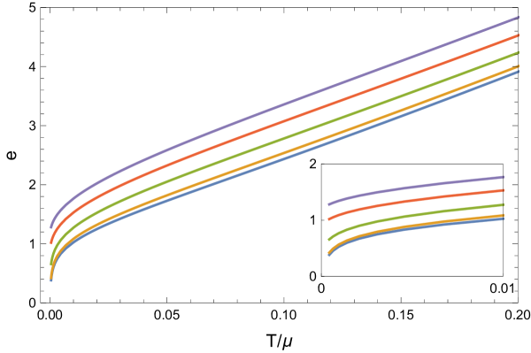
Figure 1: The charge of the scalar field versus the critical temperature for several values of the lattice amplitude. From top to down the lines represent $\lambda/\mu^{3-\Delta}=2,3/2,1,1/2,0$, where we have set $k/\mu=1/\sqrt{2}$.

• As expected, each curve shows a rise in critical temperature with charge, which is consistent with our intuition that the increase of the charge make the condensation easier, thus the critical temperature becomes higher. This tendency is the same as that in Horowitz:2013jaa .

• For a given charge, we find that increasing the lattice amplitude lowers the critical temperature, which means that the condensate of the scalar field is suppressed by the presence of the Q-lattice. Later we will find this tendency can be further confirmed by plotting the value of the condensate as a function of temperature. Such a tendency is contrary to what have been found in ionic lattice and striped superconductors, where the critical temperature is enhanced by the lattice effectsGanguli:2012up ; Horowitz:2013jaa . Preliminarily we think this discrepancy might come from the different behaviors of the chemical potential in different lattice backgrounds, as analyzed in Horowitz:2013jaa , where $\mu$ is manifestly periodic while in Q-lattice model all the fields does not manifestly depend on $x$ except the scalar field $\Phi$.

• At the zero temperature limit, not all the curves have a tendency to converge to the same point as depicted in ionic latticesHorowitz:2013jaa . On the contrary, we find when the amplitude of the lattice is large enough (which may correspond to an insulating phase before the occurrence of the condensation), these lines do not converge at least at the temperature regime that our numerical accuracy can reach (See the inset of Fig.1). It implies that for a given charge if its value is relatively small, the system with large lattice amplitude would not undergo a phase transition no matter how low the temperature is! For instance, if $e=1$, there would be no phase transition for superconductivity if $\lambda/\mu^{3-\Delta}\geq 2$ with $k/\mu=1/\sqrt{2}$, as illustrated in Fig.1.

To see more details on the dependence of the critical temperature on the lattice parameters, we may plot a 3D phase diagram on the $k-\lambda$ plane. An example is shown in the middle plot of Fig.2, where we have set $e=2$. From this figure one can obviously see that the phase transition occurs more easily in the region with small lattice amplitudes but large wavenumbers, which corresponds to the metallic phase before the transition (as is shown in the left plot of Fig.2). For a given wavenumber, the condensate becomes harder with the increase of the lattice amplitude, as illustrated in the right plot of Fig.2. While for a given lattice amplitude, the condensate becomes harder with the decrease of the wavenumber (or with the increase of the lattice constant).

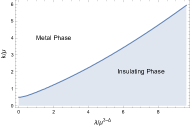
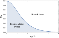
Figure 2: The left plot is a phase diagram for pure Q-lattice system without superconducting setup at extremely small temperature $T/\mu=0.001$. The middle plot is a 3D plot for the critical temperature as a function of the lattice parameters, with $e=2$. Right plot is a phase diagram for a given wave number $k/\mu=1/\sqrt{2}$.

Having found the critical temperature in a perturbative way, next we will solve all the coupled equations of motion in Eq.(3) to find Q-lattice solutions with a scalar hair at $T<T_{c}$. It involves in six ordinary differential equations with variables $U,V_{1},V_{2},\psi,\phi$ and $\eta$, which can be numerically solved with the standard pseudo-spectral method and Newton iteration. We plot the value of the condensate as a function of the temperature in Fig.3. From this figure it is obvious to see that the critical temperature for the condensation goes down when the lattice amplitude increases. Such a tendency also implies that the condensation would never occur when the amplitude is large enough and beyond some critical value. Moreover, from the right plot in Fig.3 we find the expectation value of the condensate becomes much larger in the unit of the critical temperature, implying a larger energy gap $\omega_{g}/T_{c}$ for the superconductor, which seems also different from the results in ionic lattices Horowitz:2013jaa . Finally, one can also fit the data around $T=T_{c}$ and find the expectation value behaves as $(1-T/T_{c})^{1/2}$, indicating it is the second order phase transition.

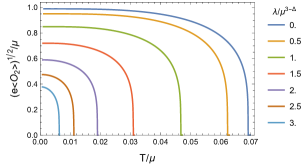
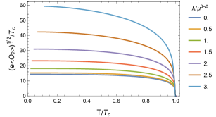
Figure 3: The value of the condensate as a function of temperature for various values of the lattice amplitude. The left plot is shown in the unit of the chemical potential while the right illustrates the same data in the unit of the critical temperature. We have set $e=2$ and $k/\mu=1/\sqrt{2}$.

In the end of this section we address the issue of the relation between the value of the condensate and the charge of the scalar field. It is known in literature that when the back-reaction is taken into account, the expectation value of the condensate which may be denoted as $\omega_{g}$ depends on the charge of the scalar fieldHartnoll:2008vx . But when $e\geq e_{c}\simeq 3\sqrt{2}$, it is found that the condensate will remain close to $\omega_{g}\sim 8\tilde{T}_{c}$. Later this universal relation has been testified in various Einstein gravity models with translational invariance. The presence of the ionic lattice drops the critical charge down to a lower value and it is found that even with $e\simeq 2$, a gap with $8T_{c}$ can be reached Horowitz:2013jaa . Now for Q-lattice background, we plot the condensate as a function of the temperature for different values of the charge in Fig.4, where we have fixed $\lambda/\mu^{3-\Delta}=1/2,3/2$, respectively and $k/\mu=1/\sqrt{2}$. One can see that the condensate will approach to $\omega_{g}\sim 9T_{c}$ when the charge $e\geq e_{c}\simeq 6$. Firstly, we have tested that this value, as found in literature, is still universal in the probe limit (namely $e\rightarrow\infty$) in our Q-lattice model and independent of the values of lattice parameters. Secondly, in comparison with the previous models we find the critical value of the charge becomes larger. As a matter of fact, for different lattice parameters $\lambda$ and $k$, we have a different value for the charge $e_{c}$ to characterize the critical region when $\omega_{g}\sim 9T_{c}$. Qualitatively, we find the larger the lattice amplitude is, the larger the critical charge $e_{c}$. This tendency is consistent with the fact that the presence of Q-lattice suppresses the condensate of the scalar field.

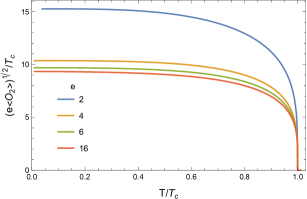
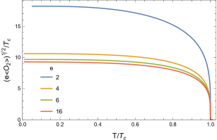
Figure 4: The value of the condensate as a function of the charge of the scalar field. Left plot we have set $\lambda/\mu^{3-\Delta}=1/2$ and $k/\mu=1/\sqrt{2}$, while right plot $\lambda/\mu^{3-\Delta}=3/2$ and $k/\mu=1/\sqrt{2}$.

IV The optical conductivity

Now we turn to compute the optical conductivity in the direction of lattice. It turns out that it is enough to consider the following consistent linear perturbation over the Q-lattice background

$$\delta g_{tx}=h_{tx}(t,z),\delta A_{x}=a_{x}(t,z),\delta\Phi=ie^{ikx}z^{3-\Delta}\varphi(t,z).$$ (7)

As stressed in Donos:2013eha , $h_{tx},a_{x}$ and $\varphi$ are real functions of $(t,z)$ such that the perturbation equations of motion will be real partial differential equations. Moreover, we suppose the fluctuations of all the fields have a time dependent form as $e^{-i\omega t}$. Thus again we are led to three ordinary differential equations for $h_{tx}(z),a_{x}(z)$ and $\varphi(z)$. Before solving these equations, we also mention that besides the boundary condition $a_{x}(0)=1$, one more boundary condition imposed at infinity is $\varphi(0)=(ik\lambda/\omega)h^{(-2)}_{tx}$ where $h^{(-2)}_{tx}$ is the coefficient of the leading order for metric expansion at infinity $h_{tx}=h^{(-2)}_{tx}/z^{2}+\cdots$. Such a boundary condition is to guarantee what we extract on the boundary for the dual field is just the current-current correlator, as investigated in Donos:2013eha . The optical conductivity is given by

$$\sigma(\omega)=\frac{\partial_{z}a_{x}(0)}{i\omega}.$$ (8)

IV.1 Superconductivity over Q-lattices dual to a metallic phase

In this subsection we discuss the optical conductivity as a function of the frequency over a Q-lattice background which is dual to a metallic phase before the phase transition. For explicitness, we fix the lattice parameters as $\lambda/\mu^{3-\Delta}=1/2$ and $k/\mu=1/\sqrt{2}$ in this subsection. We show the real and imaginary parts of the conductivity as a function of frequency for various charges in Fig.5. Our remarks on the behavior of the optical conductivity as a function of frequency can be listed as follows.

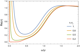
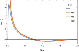
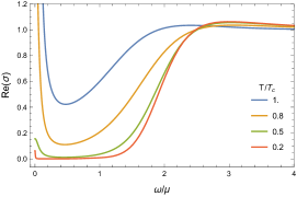
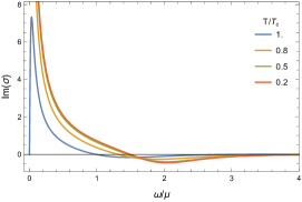
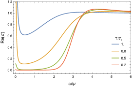
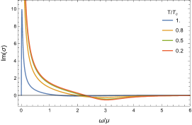
Figure 5: The real and imaginary parts of optical conductivity as a function of the frequency with $\lambda/\mu^{3-\Delta}=1/2$ and $k/\mu=1/\sqrt{2}$. From top to bottom the plots are for $e=2,4$,and $6$.

• Superconductivity. First of all, in all plots we notice that once the temperature falls below the critical temperature, the imaginary part of the conductivity will not be suppressed but climb up rapidly and exhibit a pole at $\omega=0$. Therefore, the Q-lattice does not remove the delta function in the real part of the conductivity below the critical temperature, confirming that it is dual to a genuine superconductor.

• DC conductivity due to normal fluid. The real part of the conductivity will rise at the low frequency regime as well due to the lattice effects, indicating that there is a normal component to the conductivity such that our holographic model resembles a two-fluid model. Moreover, we notice that the $DC$ conductivity will go down at first with the decrease of the temperature and then rise up to a much larger value, which can become more transparent in a log-log plot as we show in Fig.6. It means that normal component of the electron fluid is decreasing to form the superfluid component, but this normal component will not disappear quickly. The raise of the DC conductivity comes from the increase of the relaxation time, as we will describe below. In addition, when the charge becomes larger, we find that the DC conductivity starts to rise up at much lower $T/T_{c}$.

• Low frequency behavior. In low frequency region we notice that the conductivity exhibits a metallic behavior with a Drude peak even at much lower temperature. We may fit the data at low frequency with the following formula

  $$\sigma(\omega)=\frac{iK_{s}}{\omega}+\frac{K_{n}\tau}{1-i\omega\tau},$$ (9)

  where $K_{s}$ and $K_{n}$ are supposed to be proportional to the superfluid density $\rho_{s}$ and the normal fluid density $\rho_{n}$ , respectively, and $\tau$ is the relaxation time. We present a fit to this equation near the critical temperature in Fig.7 and plot the values of these parameters as a function of the temperature in Fig.8. In Fig.7 the imaginary part of the conductivity exhibits a sudden change in low frequency region when the temperature drops through the critical point. From Fig.8 we find that $K_{s}$ which is related to the superfluid density increases as the temperature goes down and becomes saturated around $T/T_{c}\simeq 0.6$, while $K_{n}$ which is related to the normal fluid density decreases rapidly below the critical temperature. However, the relaxation time does not have such a monotonous behavior. As the temperature goes down from the critical one, the relaxation time will decrease at first and then rise up quickly in low temperature region, which looks peculiar in comparison with other lattice models, where the relaxation time monotonously increases with the decreasing of the temperature. In particular, when the charge of the scalar field becomes large, the turning point moves to lower temperature region. Such a phenomenon might explain why we have a smaller DC conductivity at lower temperature as described above, since it is proportional to the relaxation time. But definitely, the issue of why the relaxation time becomes smaller at lower temperature calls for further understanding in the future. Finally, we remark that in log-log plot the Drude behavior can also be conveniently captured by a straight line with a constant slope as shown in Fig.6, which has previously been described in p-wave superconductors as well Gubser:2008wv ; Kuang:2011dy .

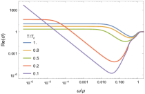
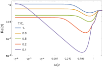
Figure 6: The Log-Log plot of the real parts of optical conductivity for Q-lattices with parameters given in Fig.5. From left to right the charge of the scalar field is taken as $e=2,4$,and $6$.

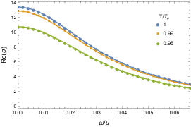
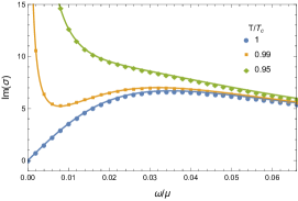
Figure 7: The critical behavior of the optical conductivity near the critical temperature. The solid lines are fits to Eq.(9).

Next we are concerned with the energy gap of the superconductor in Q-lattice model, which may be evaluated by locating the minimal value of the imaginary part of the conductivity at zero temperature limit, which may be denoted as $(\omega/\mu)_{min}$. For Q-lattices with parameters in Fig.5, we find this value corresponds to $(\omega/\mu)_{min}\simeq 18.454T_{c},10.178T_{c}$, and $9.247T_{c}$, respectively. Firstly, we find these values are comparable with the values of the condensate we obtained in the previous section and indeed they are close. Secondly, for Q-lattices with lattice amplitude $\lambda/\mu^{3-\Delta}\sim 1/2$, $(\omega/\mu)_{min}$ will be saturated around $9T_{c}$ when $e>e_{c}\simeq 6$. Finally, we have checked that the value $(\omega/\mu)_{min}\simeq 9T_{c}$ is universal in the probe limit $e\rightarrow\infty$, irrespective of the lattice parameters. In general, the energy gap in zero temperature limit does depend on the lattice parameters as well as the charge of the scalar field. However, for a given Q-lattice with fixed $\lambda/\mu^{3-\Delta}$ and $e$, we find that there always exists a critical value $e_{c}$ for the charge such that the energy gap approaches the universal value $(\omega/\mu)_{min}\simeq 9T_{c}$ when $e\geq e_{c}$, which is consistent with our analysis in the previous section on the condensate of the background.

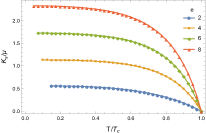
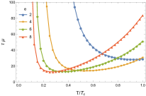
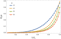
Figure 8: The three plots are $K_{s}/\mu,K_{n}/\mu$ and $\tau\mu$ as functions of the temperature.

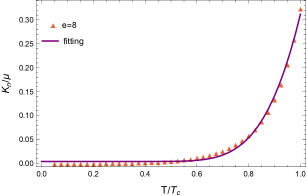
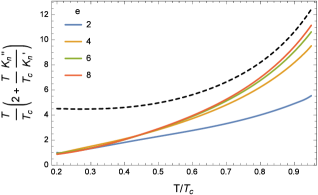
Figure 9: The first plot is the fit with Eq.(10). The second plot is for $\frac{T}{T_{c}}(2+\frac{T}{T_{c}}\frac{K_{n}^{\prime\prime}}{K_{n}^{\prime}})$ versus $T/T_{c}$, where the derivative is with respect to $T/T_{c}$. The dashed black line in the last plot is for the holographic superconductor in the absence of the Q-lattice (Note that in this case the Drude law is absent, $K_{n}$ is identified with the $DC$ conductivity.).

In literature another way to evaluate the energy gap is to fit the temperature dependence of the normal fluid density in the zero temperature limit$(\Delta/T\gg 1)$ Horowitz:2013jaa

$$\rho_{n}(T)=a+be^{-\Delta/T}.$$ (10)

In this thermodynamical method one need to know the normal fluid density at first. Usually one assumes that $\rho_{n}\propto K_{n}$ such that the normal fluid density can be obtained by fitting the conductivity with Eq.(9). Usually one expects that $(\omega/\mu)_{min}\simeq 2\Delta$ in the probe limit, which has been testified in various holographic modelsHartnoll:2008vx ; Hartnoll:2008kx ; Horowitz:2013jaa . However, in the context of Q-lattice we find such exponential behavior described by Eq.(10) is not clearly seen. The left plot of Fig.9 is an attempt to fit $K_{n}/\mu$ with Eq.(10), but obviously we notice that the data can not be well fit in the entire region. To see if the data would have an exponential behavior in any possible interval, we would better take an alternative plot as follows. If the exponential behavior would present in some region, then from Eq.(10) one would find the quantity $\frac{T}{T_{c}}(2+\frac{T}{T_{c}}\frac{K_{n}^{\prime\prime}}{K_{n}^{\prime}})$ should be a constant with value $\Delta/T_{c}$, irrespective of the value of the parameter $a$, where the derivative is with respect to $T/T_{c}$. Therefore, an exponential behavior like Eq.(10) would be featured by a horizontal line in the plot of $\frac{T}{T_{c}}(2+\frac{T}{T_{c}}\frac{K_{n}^{\prime\prime}}{K_{n}^{\prime}})$ versus $T/T_{c}$. Our results are shown in the second plot of Fig.9. In Q-lattices we do not find such behavior in any temperature region. The value of $\frac{T}{T_{c}}(2+\frac{T}{T_{c}}\frac{K_{n}^{\prime\prime}}{K_{n}^{\prime}})$ is not a constant but varies with the temperature and is obviously below the value for a system without Q-lattice in zero temperature limit. In comparison, we notice that a holographic superconductor without Q-lattice does exhibit such behavior in low temperature region, which is shown as a dashed black line and points to $\Delta/T_{c}\simeq 4.5$ as expected. Preliminarily we think this discrepancy may imply that the factor $K_{n}$ might not be related to the density $\rho_{n}$ simply by $K_{n}\propto\rho_{n}$ in Q-lattice background. Recall that in theory $K_{n}=\rho_{n}e^{2}/m^{*}$, it would be true when the effective mass of quasiparticles is also temperature dependent. This issue deserves further study in the future. In the end of this subsection we briefly address the issue of the scaling law at the mid-frequency regime. This issue has previously been investigated in both normal phase Horowitz:2012ky ; Ling:2013nxa ; Donos:2013eha ; Donos:2014yya ; Bhattacharya:2014dea and superconducting phaseHorowitz:2013jaa ; Zeng:2014uoa . It was firstly noticed in the context of scalar lattices and ionic lattices that in an intermediate frequency regime, the magnitude of the conductivity exhibits a power law behavior as

$$|\sigma(\omega)|=\frac{B}{\omega^{\gamma}}+C,$$ (11)

with $\gamma\simeq 2/3$ in four dimensional spacetime, independent of the parameters of the model. This rule has been testified in various models and in particular, its similarities with the Cuprates in superconducting phase are disclosed. However, later it is found that such a power law is not so robust in other lattice models. In particular, it was pointed out that in the context of Q-lattices there is no evidence for such an intermediate scalingDonos:2013eha . Now for the holographic superconductors in Q-lattices, we may treat it in a parallel way and our result is presented in Fig.10. From this figure, we find the intermediate scaling law is not manifest.

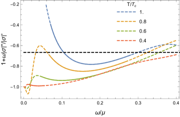
Figure 10: The plot is for $1+\omega|\sigma|^{{}^{\prime\prime}}/|\sigma|^{{}^{\prime}}$ versus $\omega/\mu$. The segment of each curve falling into the interval $2\leq\omega\tau\leq 8$ is plotted as a solid line.

IV.2 Superconductivity over Q-lattices dual to an insulating phase

In this subsection we briefly discuss the superconductivity over a Q-lattice which is dual to an insulating phase before the phase transition. We present a typical example with $\lambda/\mu^{3-\Delta}=3/2$ and $k/\mu=1/\sqrt{2}$. The optical conductivity for $e=4$ is plotted in Fig.11. In comparison with the superconductors over the Q-lattice in metallic phase, we present some general remarks as follows.

• With the decrease of the temperature, DC conductivity goes down at first and rises up again, which shares the temperature-dependence behavior with the case dual to the metallic phase.

• At low frequency, the lattice effects drive the normal electron fluid to deviate from Drude relation and exhibit an insulating behavior. This can be seen manifestly in the log-log plot in which the straight line with a constant slope becomes shorter at lower temperatures, as illustrated in the last plot of Fig.11.

• The energy gap has the same universal behavior in the probe limit, namely $(\omega/\mu)_{min}\simeq 9T_{c}$ as $e\rightarrow\infty$. For Q-lattices with parameters in Fig.11, we have $(\omega/\mu)_{min}\simeq 11.258T_{c}$, while for $e=6$, we have $9.270T_{c}$.

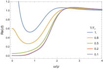
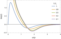
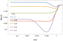
Figure 11: The real and imaginary parts of optical conductivity as a function of the frequency with $\lambda/\mu^{3-\Delta}=3/2$, $k/\mu=1/\sqrt{2}$ and $e=4$. The last one is a log-log plot for the real part.

V Discussion

In this paper we have constructed a holographic superconductor model on Q-lattice background. We have found that the lattice effects will suppress the condensate of the scalar field and thus the critical temperature becomes lower in the presence of the lattice. In particular, when the Q-lattice background is dual to a deep insulating phase, the condensate would never occur when the charge of the scalar field is relatively small. This is in contrast to the results obtained in the context of ionic lattice and striped phases, where the critical temperature is enhanced by the lattice effects. In superconducting phase it is found that the lattice does not remove the pole of the imaginary part of the conductivity, implying the existence of a delta function in the real part. The energy gap, however, depends on the lattice parameters and the charge of the scalar field. Nevertheless, in the probe limit, we find that gap $\omega_{g}\sim 9T_{c}$ is universal, irrespective of the lattice parameters. This picture is consistent with our knowledge on other sorts of holographic superconductor models.

For convenience we have only computed the optical conductivity of a superconductor where the Q-lattice background is dual to a typical metallic phase or a typical insulating phase prior to the condensation. In practice, many interesting phenomena have been explored by condensed matter experiments in the critical region where metal-insulator transition occurs in zero temperature limit. From this point of view one probably shows more interests in the superconducting behavior of the Q-lattice model with critical parameters $\lambda_{c}$ and $k_{c}$. We leave this issue for investigation in future.

This simplest model of holographic superconductors on Q-lattice can be straightforwardly generalized to other cases. For instance, we may consider to input Q-lattice structure in two spatial directions with anisotropy Ling:2014bda . We may also construct the superconductor models on Q-lattice in other gravity theories, such as the Gauss-Bonnet gravity and Einstein-Maxwell-Dilaton gravity. These works deserve further investigation.

- (1) S. S. Gubser, Phys. Rev. D 78, 065034 (2008) [arXiv:0801.2977 [hep-th]].
- (2) S. A. Hartnoll, C. P. Herzog and G. T. Horowitz, Phys. Rev. Lett. 101, 031601 (2008) [arXiv:0803.3295 [hep-th]].
- (3) S. A. Hartnoll, C. P. Herzog and G. T. Horowitz, JHEP 0812, 015 (2008) [arXiv:0810.1563 [hep-th]].
- (4) G. T. Horowitz, J. E. Santos and D. Tong, JHEP 1207, 168 (2012) [arXiv:1204.0519 [hep-th]].
- (5) G. T. Horowitz, J. E. Santos and D. Tong, JHEP 1211, 102 (2012) [arXiv:1209.1098 [hep-th]].
- (6) G. T. Horowitz and J. E. Santos, JHEP 1306, 087 (2013) [arXiv:1302.6586 [hep-th]].
- (7) S. A. Hartnoll and D. M. Hofman, Phys. Rev. Lett. 108 (2012) 241601, [arXiv:1201.3917 [hep-th]].
- (8) N. Iizuka and K. Maeda, JHEP 1211 (2012) 117, [arXiv:1207.2943 [hep-th]].
- (9) H. Ooguri and C.-S. Park, Phys. Rev. D 82 (2010) 126001, [arXiv:1007.3737 [hep-th]].
- (10) S. Kachru, A. Karch, and S. Yaida, Phys. Rev. D 81 (2010) 026007, [arXiv:0909.2639 [hep-th]].
- (11) S. Kachru, A. Karch, and S. Yaida, New J. Phys. 13 (2011) 035004, [arXiv:1009.3268 [hep-th]].
- (12) N. Bao, S. Harrison, S. Kachru, S. Sachdev, Phys. Rev. D 88 (2013) 026002 , [arXiv:1303.4390 [hep-th]].
- (13) M. R. M. Mozaffar and A. Mollabashi, Phys. Rev. D 89, no. 4, 046007 (2014) [arXiv:1307.7397 [hep-th]].
- (14) K. Wong, JHEP 1310, 148 (2013) [arXiv:1307.7839 [hep-th]].
- (15) P. Chesler, A. Lucas and S. Sachdev, Phys. Rev. D 89, 026005 (2014) [arXiv:1308.0329 [hep-th]].
- (16) D. Vegh, Holography without translational symmetry, [arXiv:1301.0537 [hep-th]].
- (17) R. A. Davison, Phys. Rev. D 88, 086003 (2013) [arXiv:1306.5792 [hep-th]].
- (18) M. Blake and D. Tong, Phys. Rev. D 88, 106004 (2013) [arXiv:1308.4970 [hep-th]].
- (19) Y. Ling, C. Niu, J. P. Wu and Z. Y. Xian, JHEP 1311, 006 (2013) [arXiv:1309.4580 [hep-th]].
- (20) B. Withers, Class. Quant. Grav. 30, 155025 (2013) [arXiv:1304.0129 [hep-th]].
- (21) T. Andrade and B. Withers, JHEP 1405, 101 (2014) [arXiv:1311.5157 [hep-th]].
- (22) B. Gout raux, JHEP 1404, 181 (2014) [arXiv:1401.5436 [hep-th]].
- (23) A. Lucas, S. Sachdev and K. Schalm, Phys. Rev. D 89, 066018 (2014) [arXiv:1401.7993 [hep-th]].
- (24) H. B. Zeng and J. P. Wu, Phys. Rev. D 90, 046001 (2014) [arXiv:1404.5321 [hep-th]].
- (25) Y. Liu, K. Schalm, Y. W. Sun and J. Zaanen, JHEP 1210, 036 (2012) [arXiv:1205.5227 [hep-th]].
- (26) Y. Ling, C. Niu, J. P. Wu, Z. Y. Xian and H. Zhang, JHEP 1307, 045 (2013) [arXiv:1304.2128 [hep-th]].
- (27) H. Ooguri and C. S. Park, Phys. Rev. Lett. 106, 061601 (2011) [arXiv:1011.4144 [hep-th]].
- (28) A. Donos and J. P. Gauntlett, JHEP 1108, 140 (2011) [arXiv:1106.2004 [hep-th]].
- (29) A. Donos and S. A. Hartnoll, Nat. Phys. 9, 649 (2013) [arXiv:1212.2998[hep-th]].
- (30) M. Rozali, D. Smyth, E. Sorkin and J. B. Stang, Phys. Rev. Lett. 110, 201603 (2013) [arXiv:1211.5600 [hep-th]].
- (31) M. Rozali, D. Smyth, E. Sorkin and J. B. Stang, Phys. Rev. D 87, 126007 (2013) [arXiv:1304.3130 [hep-th]].
- (32) A. Donos, JHEP 1305, 059 (2013) [arXiv:1303.7211 [hep-th]].
- (33) A. Donos and J. P. Gauntlett, Phys. Rev. D 87, 126008 (2013) [arXiv:1303.4398 [hep-th]].
- (34) Y. Ling, C. Niu, J. Wu, Z. Xian and H. Zhang, Phys. Rev. Lett. 113, 091602 (2014) [arXiv:1404.0777 [hep-th]].
- (35) N. Jokela, M. Jarvinen and M. Lippert, arXiv:1408.1397 [hep-th].
- (36) S. A. Hartnoll and J. E. Santos, arXiv:1403.4612 [hep-th].
- (37) A. Donos and J. P. Gauntlett, JHEP 1404, 040 (2014) [arXiv:1311.3292 [hep-th]].
- (38) S. R. Coleman, Nucl. Phys. B 262, 263 (1985) [Erratum-ibid. B 269, 744 (1986)].
- (39) A. Donos and J. P. Gauntlett, JHEP 1406, 007 (2014) [arXiv:1401.5077 [hep-th]].
- (40) A. Donos, B. Gout raux and E. Kiritsis, JHEP 1409, 038 (2014) [arXiv:1406.6351 [hep-th]].
- (41) A. Donos and J. P. Gauntlett, arXiv:1409.6875 [hep-th].
- (42) S. Ganguli, J. A. Hutasoit and G. Siopsis, Phys. Rev. D 86, 125005 (2012) [arXiv:1205.3107 [hep-th]].
- (43) R. Flauger, E. Pajer and S. Papanikolaou, Phys. Rev. D 83, 064009 (2011) [arXiv:1010.1775 [hep-th]].
- (44) J. A. Hutasoit, S. Ganguli, G. Siopsis and J. Therrien, JHEP 1202, 086 (2012) [arXiv:1110.4632 [cond-mat.str-el]].
- (45) J. A. Hutasoit, G. Siopsis and J. Therrien, JHEP 1401, 132 (2014) [arXiv:1208.2964 [hep-th]].
- (46) J. Alsup, E. Papantonopoulos and G. Siopsis, Phys. Lett. B 720, 379 (2013) [arXiv:1210.1541 [hep-th]].
- (47) J. Erdmenger, X. H. Ge and D. W. Pang, JHEP 1311, 027 (2013) [arXiv:1307.4609 [hep-th]].
- (48) X. M. Kuang, B. Wang and X. H. Ge, Mod. Phys. Lett. A 29, no. 14, 1450070 (2014) [arXiv:1307.5932 [hep-th]].
- (49) D. Arean, A. Farahi, L. A. Pando Zayas, I. S. Landea and A. Scardicchio, Phys. Rev. D 89, 106003 (2014) [arXiv:1308.1920 [hep-th]].
- (50) H. B. Zeng, Phys. Rev. D 88, 126004 (2013) [arXiv:1310.5753 [hep-th]].
- (51) S. S. Gubser and S. S. Pufu, JHEP 0811, 033 (2008) [arXiv:0805.2960 [hep-th]].
- (52) X. M. Kuang, W. J. Li and Y. Ling, Class. Quant. Grav. 29, 085015 (2012) [arXiv:1106.0784 [hep-th]].
- (53) J. Bhattacharya, S. Cremonini and B. Gout raux, arXiv:1409.4797 [hep-th].
- (54) Y. Ling, P. Liu, C. Niu, J. P. Wu and Z. Y. Xian, arXiv:1410.7323 [hep-th].