Practical Massively Parallel Sorting

Abstract

Previous parallel sorting algorithms do not scale to the largest available machines, since they either have prohibitive communication volume or prohibitive critical path length. We describe algorithms that are a viable compromise and overcome this gap both in theory and practice. The algorithms are multi-level generalizations of the known algorithms sample sort and multiway mergesort. In particular our sample sort variant turns out to be very scalable. Some tools we develop may be of independent interest – a simple, practical, and flexible sorting algorithm for small inputs working in logarithmic time, a near linear time optimal algorithm for solving a constrained bin packing problem, and an algorithm for data delivery, that guarantees a small number of message startups on each processor.

1 Introduction

Sorting is one of the most fundamental non-numeric algorithms which is needed in a multitude of applications. For example, load balancing in supercomputers often uses space-filling curves. This boils down to sorting data by their position on the curve for load balancing. Note that in this case most of the work is done for the application and the inputs are relatively small. For these cases, we need sorting algorithms that are not only asymptotically efficient for huge inputs but as fast as possible down to the range where near linear speedup is out of the question.

We study the problem of sorting $n$ elements evenly distributed over $p$ processing elements (PEs) numbered $1..p$. The output requirement is that the PEs store a permutation of the input elements such that the elements on each PE are sorted and such that no element on PE $i$ is larger than any elements on PE $i+1$.

There is a gap between the theory and practice of parallel sorting algorithms. Between the 1960s and the early 1990s there has been intensive work on achieving asymptotically fast and efficient parallel sorting algorithms. The “best” of these algorithms, e.g., Cole’s celebrated $\mathcal{O}(\log p)$ algorithm [9], have prohibitively large constant factors. Some simpler algorithms with running time $\mathcal{O}(\log^{2}p)$, however, contain interesting techniques that are in principle practical. These include parallelizations of well known sequential algorithms like mergesort and quicksort [19]. However, when scaling these algorithms to the largest machines, these algorithms cannot be directly used since all data elements are moved a logarithmic number of times which is prohibitive except for very small inputs.

For sorting large inputs, there are algorithms which have to move the data only once. Parallel sample sort [6], is a generalization of quicksort to $p-1$ splitters (or pivots) which are chosen based on a sufficiently large sample of the input. Each PE partitions its local data into $p$ pieces using the splitters and sends piece $i$ to PE $i$. After the resulting all-to-all exchange, each PE sorts its received pieces locally. Since every PE at least has to receive the $p-1$ splitters, sample sort can only by efficient for $n=\Omega(p^{2}/\log p)$, i.e., it has isoefficiency function $\Omega(p^{2}/\log p)$ (see also [21]). Indeed, the involved constant factors may be fairly large since the all-to-all exchange implies $p-1$ message startups if data exchange is done directly.

In parallel $p$-way multiway mergesort [36, 33], each PE first sorts its local data. Then, as in sample sort, the data is partitioned into $p$ pieces on each PE which are exchanged using an all-to-all exchange. Since the local data is sorted, it becomes feasible to partition the data perfectly so that every PE gets the same amount of data. Each PE receives $p$ pieces which have to be merged together. Multiway mergesort has an even worse isoefficiency function due to the overhead for partitioning.

Compromises between these two extremes – high asymptotic scalability but logarithmically many communication operations versus low scalability but only a single communication – have been considered in the BSP model [35]. Gerbessiotis and Valiant [13] develop a multi-level BSP variant of sample sort. Goodrich [14] gives communication efficient sorting algorithms in the BSP model based on multiway merging. However, these algorithms needs a significant constant factor more communications per element than our algorithms. Moreover, the BSP model allows arbitrarily fine-grained communication at no additional cost. In particular, an implementation of the global data exchange primitive of BSP that delivers messages directly has a bottleneck of $p$ message startups for every global message exchange. Also see Section 4.3 for a discussion why it is not trivial to adapt the BSP algorithms to a more realistic model of computation – it turns out that for worst case inputs, one PE may have to receive a large number of small messages.

In Section 4 we give building blocks that may also be of independent interest. This includes a distributed memory algorithm for partitioning $p$ sorted sequences into $r$ pieces each such that the corresponding pieces of each sequence can be multiway merged independently. We also give a simple and fast sorting algorithm for very small inputs. This algorithm is very useful when speed is more important than efficiency, e.g., for sorting samples in sample sort. Finally, we present an algorithm for distributing data destined for $r$ groups of PEs in such a way that all PEs in a group get the same amount of data and a similar amount of messages.

Sections 5 and 6 develop multi-level variants of multiway mergesort and sample sort respectively. The basic tuning parameter of these two algorithms is the number of (recursion) levels. With $k$ levels, we basically trade moving the data $k$ times for reducing the startup overheads to $\mathcal{O}(k\sqrt[k]{p})$. Recurse last multiway mergesort (RLM-sort) described in Section 5 has the advantage of achieving perfect load balance. The adaptive multi-level sample sort (AMS-sort) introduced in Section 6 accepts a slight imbalance in the output but is up to a factor $\log^{2}p$ faster for small inputs. A feature of AMS-sort that is also interesting for single-level algorithms is that it uses overpartitioning. This reduces the dependence of the required sample size for achieving imbalance $\varepsilon$ from $\mathcal{O}(1/\varepsilon^{2})$ to $\mathcal{O}(1/\varepsilon)$. We have already outlined these algorithms in a preprint [1].

In Section 7 we report results of an experimental implementation of both algorithms. In particular AMS-sort scales up to $2^{15}$ cores even for moderate input sizes. Multiple levels have a clear advantage over the single-level variants.

2 Preliminaries

For simplicity, we will assume all elements to have unique keys. This is without loss of generality in the sense that we enforce this assumption by an appropriate tie breaking scheme. For example, replace a key $x$ with a triple $(x,y,z)$ where $y$ is the PE number where this element is input and $z$ the position in the input array. With some care, this can be implemented in such a way that $y$ and $z$ do not have to be stored or communicated explicitly. In Appendix D we outline how this can be implemented efficiently for AMS-sort.

2.1 Model of Computation

A successful realistic model is (symmetric) single-ported message passing: Sending a message of size $\ell$ machine words takes time $\alpha+\ell\beta$. The parameter $\alpha$ models startup overhead and $\beta$ the time to communicate a machine word. For simplicity of exposition, we equate the machine word size with the size of a data element to be sorted. We use this model whenever possible. In particular, it yields good and realistic bounds for collective communication operations. For example, we get time $\mathcal{O}(\beta\ell+\alpha\log p)$ for broadcast, reduction, and prefix sums over vectors of length $\ell$ [2, 30]. However, for moving the bulk of the data, we get very complex communication patterns where it is difficult to enforce the single-ported requirement.

Our algorithms are bulk synchronous. Such algorithms are often described in the framework of the BSP model [35]. However, it is not clear how to implement the data exchange step of BSP efficiently on a realistic parallel machine. In particular, actual implementations of the BSP model deliver the messages directly using up to $p$ startups. For massively parallel machines this is not scalable enough. The BSP^∗ model [4] takes this into account by imposing a minimal message size. However, it also charges the cost for the maximal message size occurring in a data exchange for all its messages and this would be too expensive for our sorting algorithms. We therefore use our own model: We consider a black box data exchange function $\mathrm{Exch}(P,h,r)$ telling us how long it takes to exchange data on a compact subnetwork of $P$ PEs in such a way that no PE receives or sends more than $h$ words in total and at most $r$ messages in total. Note that all three parameters of the function $\mathrm{Exch}(P,h,r)$ may be essential, as they model locality of communication, bottleneck communication volume (see also [7, 29]) and startups respectively. Sometimes we also write $\smash{\mathrm{Exch}\hbox to0.0pt{\hss\raisebox{-3.0pt}{$\widetilde{\phantom{iih}}$}\hskip 3.8pt}}(P,h,r)$ as a shorthand for $(1+o(1))\mathrm{Exch}(P,h,r)$ in order to summarize a sum of $\mathrm{Exch}(\cdot)$ terms by the dominant one. We will also use that to absorb terms of the form $\mathcal{O}(\alpha\log p)$ and $\mathcal{O}(\beta r)$ since these are obvious lower bounds for the data exchange as well. A lower bound in the single-ported model for $\mathrm{Exch}(P,h,r)$ is $h\beta+r\alpha$ if data is delivered directly. There are reasons to believe that we can come close to this but we are not aware of actual matching upper bounds. There are offline scheduling algorithms which can deliver the data using time $h\beta$ when startup overheads are ignored (using edge coloring of bipartite multi-graphs). However, this chops messages into many blocks and also requires us to run a parallel edge-coloring algorithm.

2.2 Multiway Merging and Partitioning

Sequential multiway merging of $r$ sequences with total length $N$ can be done in time $\mathcal{O}(N\log r)$. An efficient practical implementation may use tournament trees [20, 27, 33]. If $r$ is small enough, this is even cache efficient, i.e., it incurs only $\mathcal{O}(N/B)$ cache faults where $B$ is the cache block size. If $r$ is too large, i.e., $r>M/B$ for cache size $M$, then a multi-pass merging algorithm may be advantageous. One could even consider a cache oblivious implementation [8].

The dual operation for sample sort is partitioning the data according to $r-1$ splitters. This can be done with the same number of comparisons and similarly cache efficiently as $r$-way merging but has the additional advantage that it can be implemented without causing branch mispredictions [32].

3 More Related Work

Figure 1: Example calculations done during fast work inefficient sorting algorithm on a $3\times 4$ array of processors. The entries in the matrix on the right show elements received from the particular row and column during the allGather, and the corresponding calculated ranks.

// select element with global rank $k$

Procedure multiSelect$(d_{1},\ldots,d_{p},k)$

if $\sum_{1\leq i\leq p}|d_{i}|=1$ then //  base case

return the only nonempty element

select a pivot $v$//  e.g. randomly

for $i$ := $1$ to $p$ dopar

find $j_{i}$ such that $d_{i}[1..j_{i}]<v$ and $d[j_{i}+1..]\geq v$

if $\sum_{1\leq i\leq p}|j_{i}|\geq k$ then

return multiSelect$(d_{1}[1..j_{1}],\ldots,d_{p}[1..j_{p}],k)$

else

return multiSelect$(d_{1}[j_{1}+1..],\ldots,d_{p}[j_{p}+1..],$

$k-\sum_{0\leq i<p}|j_{i}|)$

Figure 2: Multisequence selection algorithm.

Li and Sevcik [22] describe the idea of overpartitioning. However, they use centralized sorting of the sample and a master worker load balancer dealing out buckets for sorting in order of decreasing bucket size. This leads to very good load balance but is not scalable enough for our purposes and heuristically disperses buckets over all PEs. Achieving the more strict output format that our algorithm provide would require an additional complete data exchange. Our AMS-sort from Section 6 is fully parallelized without sequential bottlenecks and optimally partitions consecutive ranges of buckets.

A state of the art practical parallel sorting algorithm is described by Solomonik and Kale [34]. This single level algorithm can be viewed as a hybrid between multiway mergesort and (deterministic) sample sort. Sophisticated measures are taken for overlapping internal work and communication. TritonSort [26] is a very successful sorting algorithm from the database community. TritonSort is a version of single-level sample-sort with centralized generation of splitters.

4 Building Blocks

4.1 Multisequence Selection

In its simplest form, given sorted sequences $d_{1},\ldots,d_{p}$ and a rank $k$, multisequence selection asks for finding an element $x$ with rank $k$ in the union of these sequences. If all elements are different, $x$ also defines positions in the sequences such that there is a total number of $k$ elements to the left of these positions.

There are several algorithms for multisequence selection, e.g. [36, 33]. Here we propose a particularly simple and intuitive method based on an adaptation of the well-known quick-select algorithm [16, 24]. This algorithm may be folklore. The algorithm has also been on the publicly available slides of Sanders’ lecture on parallel algorithms since 2008 [28]. Figure 2 gives high level pseudo code. The base case occurs if there is only a single element (and $k=1$). Otherwise, a random element is selected as a pivot. This can be done in parallel by choosing the same random number between 1 and $\sum_{i}|d_{i}|$ on all PEs. Using a prefix sum over the sizes of the sequences, this element can be located easily in time $\mathcal{O}(\alpha\log p)$. Where ordinary quickselect has to partition the input doing linear work, we can exploit the sortedness of the sequences to obtain the same information in time $\mathcal{O}(\log D)$ with $D:=\max_{i}|d_{i}|$ by doing binary search in parallel on each PE. If items are evenly distributed, we have $D=\Theta(\frac{n}{p})$, and thus only time $\mathcal{O}(\log\frac{n}{p})$ for the search, which partitions all the sequences into two parts. Deciding whether we have to continue searching in the left or the right parts needs a global reduction operation taking time $\mathcal{O}(\alpha\log p)$. The expected depth of the recursion is $\mathcal{O}(\log\sum_{i}|d_{i}|)=\mathcal{O}(\log n)$ as in ordinary quickselect. Thus, the overall expected running time is $\mathcal{O}((\alpha\log p+\log\frac{n}{p})\log n)$.

In our application, we have to perform $r$ simultaneous executions of multisequence selection on the same input sequences but on $r$ different rank values. The involved collective communication operations will then get a vector of length $r$ as input and their running time using an asymptotically optimal implementation is $\mathcal{O}(r\beta+\alpha\log p)$ [2, 30]. Hence, the overall running time of multisequence selection becomes

$$\mathcal{O}((\alpha\log p+r\beta+r\log\tfrac{n}{p})\log n)\enspace.$$ (1)

4.2 Fast Work Inefficient Sorting

We generalize an algorithm from [18] which may also be considered folklore. In its most simple form, the algorithm arranges $n^{2}$ PEs as a square matrix using PE indices from $1..n\times 1..n$. Input element $i$ is assumed to be present at PE $(i,i)$ initially. The elements are first broadcast along rows and columns. Then, PE $(i,j)$ computes the result of comparing elements $i$ and $j$ (0 or 1). Summing these comparison results over row $i$ yields the rank of element $i$.

Our generalization works for a rectangular $a\times b$ array of processors where $a=\mathcal{O}(\sqrt{p})$ and $b=\mathcal{O}(\sqrt{p})$. In particular, when $p=2^{P}$ is a power of two, then $a=2^{\left\lceil P/2\right\rceil}$ and $b=2^{\left\lfloor P/2\right\rfloor}$. Initially, there are $n$ elements uniformly distributed over the PEs, i.e. each PE has at most $\left\lceil n/p\right\rceil$ elements as inputs. These are first sorted locally in time $\mathcal{O}(\frac{n}{p}\log\frac{n}{p})$.

Then the locally sorted elements are gossiped (allGather) along both rows and columns (see Figure 1), making sure that the received elements are sorted. This can be achieved in time $\mathcal{O}(\alpha\log p+\beta\frac{n}{\sqrt{p}})$. For example, if the number of participating PEs is a power of two, we can use the well known hypercube algorithm for gossiping (e.g., [21]). The only modification is that received sorted sequences are not simply concatenated but merged.

Figure 3: Exchange schema without and with first stage: permutation of PEs

Figure 4: Deterministic data delivery schema

Elements received from column $i$ are then ranked with respect to the elements received from row $j$. This can be done in time $\mathcal{O}(\frac{n}{\sqrt{p}})$ by merging these two sequences. Summing these local ranks along rows then yields the global rank of each element. If desired, this information can then be used for routing the input elements in such a way that a globally sorted output is achieved. In our application this is not necessary because we want to extract elements with certain specified ranks as a sample. Either way, we get overall execution time

$$\mathcal{O}\!\left(\alpha\log p+\beta\tfrac{n}{\sqrt{p}}+\tfrac{n}{p}\log\tfrac{n}{p}\right)\enspace.$$ (2)

Note that for $n$ polynomial in $p$ this bound is $\mathcal{O}(\alpha\log p+\beta\frac{n}{\sqrt{p}})$. This restrictions is fulfilled for all reasonable applications of this sorting algorithm.

4.3 Delivering Data to the Right Place

In the sorting algorithms considered here we face the following data redistribution problem: Each PE has partitioned its locally present data into $r$ pieces. The pieces with number $i$ have to be moved to PE group $i$ which consists of PEs $(i-1)r+1..ir$. Each PE in a group should receive the same amount of data except for rounding issues.

We begin with a simple approach and then refine it in order to handle bad cases. The basic idea is to compute a prefix sum over the piece sizes – this is a vector-valued prefix sum with vector length $r$. As a result, each piece is labeled with a range of positions within the group it belongs to. Positions are numbers between $1$ and $m_{i}$ where $m_{i}\leq n/r$ is the number of elements assigned to group $i$. An element with number $j$ in group $i$ is sent to PE $(i-1)\frac{p}{r}+\lceil\frac{j}{m_{i}}\rceil$. This way, each PE sends exactly $n/p$ elements and receives at most $\left\lceil m_{i}r/p\right\rceil$ elements. Moreover, each piece is sent to one or two target PEs responsible for handling it in the recursion. Thereby, each PE sends at most $2r$ messages for the data exchange. Unfortunately, the number of received messages, although the same on the average, may vary widely in the worst case. There are inputs where some PEs have to receive $\Omega(p)$ very small pieces. This happens when many consecutively numbered PEs send only very small pieces of data (see PE 9 in the top of Figure 3).

One way to limit the number of received pieces is to use randomization. We describe how to do this while keeping the data perfectly balanced. We describe this approach in two stages where already the first, rather simple stage gives a significant improvement. The first stage is to choose the PE-numbering used for the prefix sum as a (pseudo)random permutation within each group (see Appendix B). However, it can be shown that if all but $p/r$ pieces are very small, this would still imply a logarithmic factor higher startup overheads for the data exchange at some PEs. In Appendix A we give an advanced randomized algorithm that gets rid of this logarithmic factor. But now we give an algorithm that is deterministic and at least conceptually simpler.

4.3.1 A Deterministic Solution

The basic idea is to distribute small and large pieces separately. In Figure 4 we illustrate the process. First, small pieces of size at most $n/2pr$ are enumerated using a prefix sum. Small piece $i$ of group $j$ is assigned to PE $\left\lfloor i/r\right\rfloor$ of group $j$. This way, all small pieces are assigned without having to split them and no receiving PE gets more than half its final load.

In the second phase, the remaining (large) pieces are assigned taking the residual capacity of the PEs into account. PE $i$ sends the description of its piece for group $j$ to PE $\left\lfloor i/r\right\rfloor$ of group $j$. This can be done in time $\mathrm{Exch}(p,\mathcal{O}(r),r)$. Now, each group produces an assignment of its large pieces independently, i.e., each group of $p/r$ PEs assigns up to $p$ pieces – $r$ on each PE. In the following, we describe the assignment process for a single group.

Figure 5: Algorithm schema of Recurse Last Parallel Multiway Mergesort

Conceptually, we enumerate the unassigned elements on the one hand and the unassigned slots able to take them on the other hand and then map element $i$ to slot $i$. To implement this, we compute a prefix sum of the residual capacities of the receiving PEs on the one hand and the sizes of the unassigned pieces of the other hand. This yields two sorted sequences $X$ and $Y$ respectively which are merged in order to locate the destination PEs of each large piece. Assume that ties in values of $X$ and $Y$ are broken such that elements from $X$ are considered smaller. In the merged sequence, a subsequence of the form $\left\langle x_{i},y_{j},\ldots,y_{j+k},x_{i+1},z\right\rangle$ indicates that pieces $j,\ldots,j+k$ have to moved to PE $i$. Piece $j+k$ may also wrap over to PE $i+1$, and possibly to PE $i+2$ if $z=x_{i+2}$. The assumptions on the input guarantee that no further wrapping over is possible since no piece can be larger than $n/p$ and since every PE has residual capacity at least $\frac{n}{2p}$. Similarly, since large pieces have size at least $n/2pr$ and each PE gets assigned at most $n/p$ elements, no PE gets more than $\frac{n}{p}/\frac{n}{2pr}=2r$ large pieces.

The difficult part is merging the two sorted sequences $X$ and $Y$. Here one can adapt and simplify the work efficient parallel merging algorithm for EREW PRAMs from [15]. Essentially, one first merges the $p/r$ elements of $X$ with a deterministic sample of $Y$ – we include the prefix sum for the first large piece on each PE into $Y$. This merging operation can be done in time $\mathcal{O}(\alpha\log(p/r))$ using Batcher’s merging network [3]. Then each element of $X$ has to be located within the $\leq r$ local elements of $Y$ on one particular PE. Since it is impossible that these pieces (of total size $\leq rn/p$) fill more than $2r$ PEs (of residual capacity $>n/2p$), each PE will have to locate only $\mathcal{O}(r)$ elements. This can be done using local merging in time $\mathcal{O}(r)$. In other words, the special properties of the considered sequence make it unnecessary to perform the contention resolution measures making [15] somewhat complicated. Overall, we get the following deterministic result (recall from Section 2.1 that $\smash{\mathrm{Exch}\hbox to0.0pt{\hss\raisebox{-3.0pt}{$\widetilde{\phantom{iih}}$}\hskip 3.8pt}}(\cdot)$ also absorbs terms of the form $\mathcal{O}(\alpha\log p+\beta r)$).

Theorem 1

Data delivery of $r\times p$ pieces to $r$ parts can be implemented to run in time

$$\smash{\mathrm{Exch}\hbox to0.0pt{\hss\raisebox{-3.0pt}{$\widetilde{\phantom{iih}}$}\hskip 3.8pt}}(p,\tfrac{n}{p},\mathcal{O}(r))\enspace.$$

5 Generalizing Multilevel Mergesort (RLM-Sort)

We subdivide the PEs into “natural” groups of size $p^{\prime}$ on which we want to recurse. Asymptotically, $r\mbox{\rm:= }p/p^{\prime}$ around $\sqrt[k]{p}$ is a good choice if we want to make $k$ levels of recursion. However, we may also fix $p^{\prime}$ based on architectural properties. For example, in a cluster of many-core machines, we might chose $p^{\prime}$ as the number of cores in one node. Similarly, if the network has a natural hierarchy, we will adapt $p^{\prime}$ to that situation. For example, if PEs within a rack are more tightly connected than inter-rack connections, we may choose $p^{\prime}$ to be the number of PEs within a rack. Other networks, e.g., meshes or tori have less pronounced cutting points. However, it still makes sense to map groups to subnetworks with nice properties, e.g., nearly cubic subnetworks. For simplicity, we will assume that $p$ is divisible by $p^{\prime}$, and that $r=\Theta(\sqrt[k]{p})$.

There are several ways to define multilevel multiway mergesort. We describe a method we call “recurse last” (see Figure 5) that needs to communicate the data only $k$ times and avoids problems with many small messages. Every PE sorts locally first. Then each of these $p$ sorted sequences is partitioned into $r$ pieces in such a way that the sum of these piece sizes is $n/r$ for each of these $r$ resulting parts. In contrast to the single level algorithm, we run only $r$ multisequence selections in parallel and thus reduce the bottleneck due to multisequence selection by a factor of $p^{\prime}$.

Now we have to move the data to the responsible groups. We defer to Section 4.3 which shows how this is possible using time $\smash{\mathrm{Exch}\hbox to0.0pt{\hss\raisebox{-3.0pt}{$\widetilde{\phantom{iih}}$}\hskip 3.8pt}}(p,\frac{n}{p},\mathcal{O}(\sqrt[k]{p}))$.

Afterwards, group $i$ stores elements which are no larger than any element in group $i+1$ and it suffices to recurse within each group. However, we do not want to ignore the information already available – each PE stores not an entirely unsorted array but a number of sorted sequences. This information is easy to use though – we merge these sequences locally first and obtain locally sorted data which can then be subjected to the next round of splitting.

Figure 6: Algorithm schema of AMS-sort

Theorem 2

RLM-sort with $k=\mathcal{O}(1)$ levels of recursion can be implemented to run in time

$$\mathcal{O}\!\left(\left(\alpha\log p+\sqrt[k]{p}\;\beta+\sqrt[k]{p}\,\log\tfrac{n}{p}+\tfrac{n}{p}\right)\log n\right)+$$

$${\sum_{i=1}^{k}}\,\smash{\mathrm{Exch}\hbox to0.0pt{\hss\raisebox{-3.0pt}{$\widetilde{\phantom{iih}}$}\hskip 3.8pt}}\left(p^{\frac{i}{k}},\tfrac{n}{p},\mathcal{O}\!\left(\sqrt[k]{p}\right)\right)\enspace.$$ (3)

Proof 5.3.

(Outline) Local sorting takes time $\mathcal{O}(\frac{n}{p}\log n)$. For $k=\mathcal{O}(1)$ multiselections we get the bound from Equation (1), $\mathcal{O}((\alpha\log p+r\beta+r\log\tfrac{n}{p})\log n)$. Summing the latter two contributions, we get the first term of Equation (3).

In level $i$ of the recursion we have $r^{i}$ independent groups containing $\frac{p}{r^{i}}=\frac{p}{p^{i/k}}=p^{1-\frac{i}{k}}$ PEs each. An exchange within the group in level $i$ costs $\smash{\mathrm{Exch}\hbox to0.0pt{\hss\raisebox{-3.0pt}{$\widetilde{\phantom{iih}}$}\hskip 3.8pt}}(p^{1-i/k},\frac{n}{p},\mathcal{O}(\frac{r}{r^{i}}))$ time. Since all independent exchanges are performed simultaneously, we only need to sum over the $k$ recursive levels, which yields the second term of Equation (3).

Equation (3) is a fairly complicated expression but using some reasonable assumptions we can simplify it. If all communications are equally expensive, the sum becomes $k\smash{\mathrm{Exch}\hbox to0.0pt{\hss\raisebox{-3.0pt}{$\widetilde{\phantom{iih}}$}\hskip 3.8pt}}(p,\frac{n}{p},\mathcal{O}(\sqrt[k]{p}))$ – we have $k$ message exchanges involving all the data but we limit the number of startups to $\mathcal{O}(\sqrt[k]{p})$. On the other hand, on mesh or torus networks, the first (global) exchange will dominate the cost and we get $\smash{\mathrm{Exch}\hbox to0.0pt{\hss\raisebox{-3.0pt}{$\widetilde{\phantom{iih}}$}\hskip 3.8pt}}(p,\frac{n}{p},\mathcal{O}(\sqrt[k]{p}))$ for the sum. If we also assume that data is delivered directly, $\Omega(\sqrt[k]{p})$ startups hidden in the $\smash{\mathrm{Exch}\hbox to0.0pt{\hss\raisebox{-3.0pt}{$\widetilde{\phantom{iih}}$}\hskip 3.8pt}}()$ term will dominate the $\mathcal{O}(\log^{2}p)$ startups in the remaining algorithm. We can assume that $n$ is bounded by a polynomial in $p$ – otherwise, a traditional single-phase multi-way mergesort would be a better algorithm. This implies that $\log n=\Theta(\log p)$. Furthermore, if $n=\omega(p^{1+1/k}\log p)$ then $n/p=\omega(p^{\frac{1}{k}}\log p)$, and the term $\Omega(\beta\frac{n}{p})$ hidden in the data exchange term dominates the term $\mathcal{O}(\beta p^{\frac{1}{k}}\log n)$. Thus Equation (3) simplifies to $\mathcal{O}(\frac{n}{p}\log n)$ (essentially the time for internal sorting) plus the data exchange term.

If we also assume $\alpha$ and $\beta$ to be constants and estimate $\smash{\mathrm{Exch}\hbox to0.0pt{\hss\raisebox{-3.0pt}{$\widetilde{\phantom{iih}}$}\hskip 3.8pt}}$-term as $\mathcal{O}(\frac{n}{p})$, we get execution time

$$\mathcal{O}(\sqrt[k]{p}\log^{2}p+\frac{n}{p}\log n)\enspace.$$

From this, we can infer a $\mathcal{O}(p^{1+1/k}\log p)$ as isoefficiency function.

6 Adaptive Multi-Level
Sample Sort (AMS-Sort)

A good starting point is the multi-level sample sort algorithm by Gerbessiotis and Valiant [13]. However, they use centralized sorting of the sample and their data redistribution may lead to some processors receiving $\Omega(p)$ messages (see also Section 4.3). We improve on this algorithm in several ways to achieve a truly scalable algorithm. First, we sort the sample using fast parallel sorting. Second, we use the advanced data delivery algorithms described in Section 4.3, and third, we give a scalable parallel adaptation of the idea of overpartitioning [22] in order to reduce the sample size needed for good load balance.

But back to our version of multi-level sample sort (see Figure 6). As in RLM-sort, our intention is to split the PEs into $r$ groups of size $p^{\prime}=p/r$ each, such that each group processes elements with consecutive ranks. To achieve this, we choose a random sample of size $abr$ where the oversampling factor $a$ and the overpartitioning factor $b$ are tuning parameters. The sample is sorted using a fast sorting algorithm. We assume the fast inefficient algorithm from Section 4.2. Its execution time is $\mathcal{O}(\frac{abr}{p}\log\frac{abr}{p}+\beta\frac{abr}{\sqrt{p}}+\alpha\log p)$.

From the sorted sample, we choose $br-1$ splitter elements with equidistant rank. These splitters are broadcast to all PEs. This is possible in time $\mathcal{O}(\beta br+\alpha\log p)$.

Then every PE partitions its local data into $br$ buckets corresponding to these splitters. This takes time $\mathcal{O}(\frac{n}{p}\log(br))$.

Using a global (all-)reduction, we then determine global bucket sizes in time $\mathcal{O}(\beta br+\alpha\log p)$. These can be used to assign buckets to PE-groups in a load balanced way: Given an upper bound $L$ on the number of elements per PE-group, we can scan through the array of bucket sizes and skip to the next PE-group when the total load would exceed $L$. Using binary search on $L$ this finds an optimal value for $L$ in time $\mathcal{O}(br\log n)$ using a sequential algorithm. In Appendix C we explain how this can be improved to $\mathcal{O}(br\log br)$ and, using parallelization, even to $\mathcal{O}(br+\alpha\log p).$

Lemma 6.4.

The above binary search scanning algorithm indeed finds the optimal $L$.

Proof 6.5.

We first show that binary search suffices to find the optimal $L$ for which the scanning algorithm succeeds. Let $L^{*}$ denote this value. For this to be true, it suffices to show that for any $L\geq L^{*}$, the scanning algorithm finds a feasible partition into groups with load at most $L$. This works because the scanning algorithm maintains the invariant that after defining $i$ groups, the algorithm with bound $L$ has scanned at least as many buckets as the algorithm with bound $L^{*}$. Hence, when the scanning algorithm with bound $L^{*}$ has defined all groups, the one with bound $L$ has scanned at least as many buckets as the algorithm with bound $L^{*}$. Applying this invariant to the final group yields the desired result.

Now we prove that no other algorithm can find a better solution. Let $L^{*}$ denote the maximum group size of an optimal partitioning algorithm. We argue that the scanning algorithm with bound $L^{*}$ will succeed. We now compare any optimal algorithm with the scanning algorithm. Consider the first $i$ buckets defined by both algorithms. It follows by induction on $i$ that the total size $s^{s}_{i}$ of these buckets for the scanning algorithm is at least as large as the corresponding value $s^{*}_{i}$ for the optimal algorithm: This is certainly true for $i=0$ ($s^{s}_{0}=s^{*}_{0}=0$). For the induction step, suppose that the optimal algorithm chooses a bucket of size $y$, i.e., $s^{*}_{x+1}=s^{*}_{x}+y$. By the induction hypothesis, we know that $s^{s}_{i}\geq s^{*}_{i}$. Now suppose, the induction invariant would be violated for $i+1$, i.e., $s^{s}_{i+1}<s^{*}_{i+1}$. Overall, we get $s^{*}_{i}\leq s^{s}_{i}<s^{s}_{i+1}<s^{*}_{i+1}$. This implies that $s^{s}_{i+1}-s^{s}_{i}$ – the size of group $i+1$ for the scanning algorithm – is smaller than $y$. Moreover, this group contains a proper subset of the buckets included by the optimal algorithm. This is a impossible since there is no reason why the scanning algorithm should not at least achieve a bucket size $s^{*}_{i+1}-s^{s}_{i}\leq y\leq L^{*}$.

Lemma 6.6.

We can achieve $L=(1+\varepsilon)\frac{n}{r}$ with high probability choosing appropriate $b=\Omega(1/\varepsilon)$ and $ab=\Omega(\log r)$.

Proof 6.7.

We only give the basic idea of a proof. We argue that the scanning algorithm is likely to succeed with $L=(1+\varepsilon)\frac{n}{r}$ as a group size limit. Using Chernoff bounds it can be shown that $ab=\Omega(\log p)$ ensures that no bucket has size larger than $\frac{n}{r}$ with high probability. Hence, the scanning algorithm can always build feasible PE groups from one or multiple buckets.

Choosing $b\geq 2/\varepsilon$ means that the expected bucket size is $\leq\frac{\varepsilon}{2}\cdot\frac{n}{r}$. Indeed, most elements will be in buckets of size less than $\varepsilon\frac{n}{r}$. Hence, when the scanning algorithm adds a bucket to a PE-group such that the average group size $\frac{n}{r}$ is passed for the first time, most of the time this additional group will also fit below the limit of $(1+\varepsilon)\frac{n}{r}$. Overall, the scanning algorithm will mostly form groups of size exceeding $\frac{n}{r}$ and thus $r$ groups will suffice to cover all buckets of total size $n$.

The data splitting defined by the bucket group is then the input for the data delivery algorithm described in Section 4.3. This takes time $\smash{\mathrm{Exch}\hbox to0.0pt{\hss\raisebox{-3.0pt}{$\widetilde{\phantom{iih}}$}\hskip 3.8pt}}\left(p,(1+o(1))L,(2+o(1))r\right)$).

We recurse on the PE-groups similar to Section 5. Within the recursion it can be exploited that the elements are already partitioned into $br$ buckets.

We get the following overall execution time for one level:

Lemma 6.8.

One level of AMS-sort works in time

$$\mathcal{O}\!\left(\frac{n}{p}\log\frac{r}{\varepsilon}+\beta\frac{r}{\varepsilon}\right)+\smash{\mathrm{Exch}\hbox to0.0pt{\hss\raisebox{-3.0pt}{$\widetilde{\phantom{iih}}$}\hskip 3.8pt}}(p,(1+\varepsilon)\tfrac{n}{p},\mathcal{O}(r))\enspace.$$ (4)

Proof 6.9.

(Outline) This follows from Lemma 6.6 and the individual running times described above using $ab=\Theta(\max(\log r,1/\varepsilon))$, $b=\Theta(1/\varepsilon)$, and fast inefficient sorting for sorting the sample. The sample sorting term then reads $\mathcal{O}(\frac{abr}{p}\log\frac{abr}{p}+\beta\frac{abr}{\sqrt{p}}+\alpha\log p)$ which is $o(\frac{n}{p}\log\frac{r}{\epsilon}+\frac{\beta}{\varepsilon})+\alpha\log p$. Note that the term $\alpha\log p$ is absorbed into the $\smash{\mathrm{Exch}\hbox to0.0pt{\hss\raisebox{-3.0pt}{$\widetilde{\phantom{iih}}$}\hskip 3.8pt}}$-term.

Compared to previous implementations of sample sort, including the one from Gerbessiotis and Valiant [13], AMS-sort improves the sample size from $\mathcal{O}(p\log p/\varepsilon^{2})$ to $\mathcal{O}(p(\log r+1/\varepsilon))$ and the number of startup overheads in the $\mathrm{Exch}$-term from $\mathcal{O}(p)$ to $\mathcal{O}(r)$.

In the base case of AMS-sort, when the recursion reaches a single PE, the local data is sorted sequentially.

Theorem 6.10.

Adaptive multi-level sample sort (AMS-sort) with $k$ levels of recursion and a factor $(1+\varepsilon)$ imbalance in the output can be implemented to run in time

$$\mathcal{O}\!\left(\frac{n}{p}\log n+\beta\frac{k^{2}\sqrt[k]{p}}{\varepsilon}\right)+{\sum_{i=1}^{k}}\,\smash{\mathrm{Exch}\hbox to0.0pt{\hss\raisebox{-3.0pt}{$\widetilde{\phantom{iih}}$}\hskip 3.8pt}}\left(p^{\frac{i}{k}},(1+\varepsilon)\tfrac{n}{p},\mathcal{O}\!\left(\sqrt[k]{p}\right)\right)$$

if $k=\mathcal{O}(\log p/\log\log p)$ and $\frac{1}{\varepsilon}=\mathcal{O}(\sqrt[k]{n})$.

Proof 6.11.

We choose $r=\sqrt[k]{p}$. Since errors multiply, we choose $\varepsilon^{\prime}=\sqrt[k]{1+\varepsilon}-1=\Theta(\frac{\varepsilon}{k})$ as the balance parameter for each level. Using Lemma 6.8 we get the following terms.
For internal computation: $\mathcal{O}(\frac{n}{p})\log n$ for the final internal sorting. (We do not exploit that overpartitioning presorts the data to some extent.) For partitioning, we apply Lemma 6.8 and get time

$$\mathcal{O}\!\left(k\log\frac{r}{\epsilon^{\prime}}\right) =\mathcal{O}\!\left(k\frac{n}{p}\log\frac{k\sqrt[k]{p}}{\varepsilon}\right)$$

$$=\frac{n}{p}\mathcal{O}\!\left(\log p+k\log k+k\log\frac{1}{\varepsilon}\right)$$ (5)

$$=\frac{n}{p}\mathcal{O}\!\left(\log p+\log n\right)\enspace.$$

The last estimate uses the preconditions $k=\mathcal{O}(\log p/\log\log p)$ and $\frac{1}{\varepsilon}=\mathcal{O}(\sqrt[k]{n})$ in order to simplify the theorem.

For communication volume we get $k\cdot\beta\frac{r}{\varepsilon^{\prime}}=\mathcal{O}(\beta\frac{k^{2}\sqrt[k]{p}}{\varepsilon})$. For startup latencies we get $\mathcal{O}(\alpha k\log p)$ which can be absorbed into the $\smash{\mathrm{Exch}\hbox to0.0pt{\hss\raisebox{-3.0pt}{$\widetilde{\phantom{iih}}$}\hskip 3.8pt}}()$-terms.

The data exchange term is the same as for RLM-sort except that we have a slight imbalance in the communication volume.

Using a similar argument as for RLM-sort, for constant $k$ and $\varepsilon$, we get an isoefficiency function of $p^{1+1/k}/\log p$ for $r=\sqrt[k]{p}$. This is a factor $\log^{2}p$ better than for RLM-sort and is an indication that AMS-sort might be the better algorithm – in particular if some imbalance in the output is acceptable and if the inputs are rather small.

Another indicator for the good scalability of AMS-sort is that we can view it as a generalization of parallel quicksort that also works efficiently for very small inputs. For example, suppose $n=\mathcal{O}(p\log p)$ and $1/\varepsilon=\mathcal{O}(1)$. We run $k=\mathcal{O}(\log p)$ levels of AMS-sort with $r=\mathcal{O}(1)$ and $\varepsilon^{\prime}=\mathcal{O}(k/\varepsilon)$. This yields running time $\mathcal{O}(\log^{2}p\log\log p+\alpha\log^{2}p)$ using the bound from Equation (5) for the local work. This does a factor $\mathcal{O}(\log\log p)$ more local work than an asymptotically optimal algorithm. However, this is likely to be irrelevant in practice since it is likely that $\alpha\gg\log\log p$. Also the factor $\log\log p$ would disappear in an implementation that exploits the information gained during bucket partitioning.

7 Experimental Results

We now present the results of our AMS-sort and RLM-sort experiments. In our experiments we run a weak scaling benchmark, which shows how the wall-time varies for an increasing number of processors for a fixed amount of elements per processor. Furthermore, in Appendix E we show additional experiments considering the effect of overpartitioning in more detail. The test covers the AMS-sort and RLM-sort algorithms executed with $10^{5}$, $10^{6}$, and $10^{7}$ 64-bit integers. We ran our experiments at the thin node cluster of the SuperMUC (www.lrz.de/supermuc), a island-based distributed system consisting of $18$ islands, each with 512 computation nodes. However, the maximum number of islands available to us was four. Each computation node has two Sandy Bridge-EP Intel Xeon E5-2680 8-core processors with a nominal frequency of $2.7$ GHz and $32$ GByte of memory. However, jobs will run at the standard frequency of $2.3$ GHz as the LoadLeveler does not classify the implementation as accelerative based on the algorithm’s energy consumption and runtime. A non-blocking topology tree connects the nodes within an island using the Infiniband FDR10 network technology. Computation nodes are connected to the non-blocking tree by Mellanox FDR ConnectX-3 InfiniBand mezzanine adapters. A pruned tree connects the islands among each other with a bi-directional bi-section bandwidth ratio of $4:1$. The interconnect has a theoretical bisection bandwidth of up to $35.6$ TB/s.

7.1 Implementation Details

We implemented AMS-sort and RLM sort in C++ with the main objective to demonstrate that multilevel algorithms can be useful for large $p$ and moderate $n$. We use naive prefix-sum based data delivery without randomization since we currently only use random inputs anyway – for these the naive algorithm coincides with the deterministic algorithm since all pieces are large with high probability.

AMS-sort implements overpartitioning, however using the simple sequential algorithm for bucket grouping which incurs an avoidable factor $\mathcal{O}(\log n)$. Also, information stemming from overpartitioning is not yet exploited for the recursive subproblems. This means that overpartitioning is not yet as effective as it would be in a full-fledged implementation.

We divide each level of the algorithms into four distinct phases: splitter selection, bucket processing (multiway merging or distribution), data delivery, and local sorting. To measure the time of each phase, we place a MPI barrier before each phase. Timings for these phases are accumulated over all recursion levels.

The time for building MPI communicators (which can be considerable) is not included in the running time since this can be viewed as a precomputation that can be reused over arbitrary inputs.

The algorithms are written in C++11 and compiled with version $15.0$ of the Intel icpc compiler, using the full optimization flag -O3 and the instruction set specified with -march=corei7-avx. For inter-process communication, we use version version $1.3$ of the IBM mpich2 library.

During the bucket processing phase of RLM-sort, we use the sequential_multiway_merge implementation of the GNU Standard C++ Library to merge buckets [33]. We used our own implementation of multisplitter partitioning in the bucket processing phase, borrowed from super scalar sample sort [32].

For the data delivery phase, we use our own implementation of a 1-factor algorithm [31] and compare it against the all-to-allv implementation of the IBM mpich2 library. The 1-factor implementation performs up to $p$ pairwise MPI_Isend and MPI_Irecv operations to distribute the buckets to their target groups. In contrast to the mpich2 implementation, the 1-factor algorithm omits the exchange of empty messages. We found that the 1-factor implementation is more stable and exchanges data with a higher throughput on the average. Local sorting uses std::sort.

7.2 Weak Scaling Analysis

	level	$p$
$k$		$512$	$2048$	$8192$	$32768$
$1$	1	$16$	$16$	$16$	$16$
$2$	1	$32$	$128$	$512$	$2048$
	2	$16$	$16$	$16$	$16$
$3$	1	$8$	$16$	$32$	$64$
	2	$4$	$8$	$16$	$32$
	3	$16$	$16$	$16$	$16$

Table 1: Selection of $r$ for weak scaling experiments

	$p$
$n/p$	$512$	$2048$	$8192$	$32768$
$10^{5}$	$0.0228$	$0.0277$	$0.0359$	$0.0707$
$10^{6}$	$0.2212$	$0.2589$	$0.2687$	$0.9171$
$10^{7}$	$2.6523$	$2.9797$	$4.0625$	$6.0932$

Table 2: AMS-sort median wall-times of weak scaling experiments in seconds

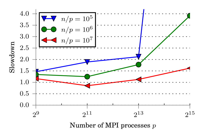
Figure 7: Slowdown of RLM-sort compared to AMS-sort based on optimal level choice

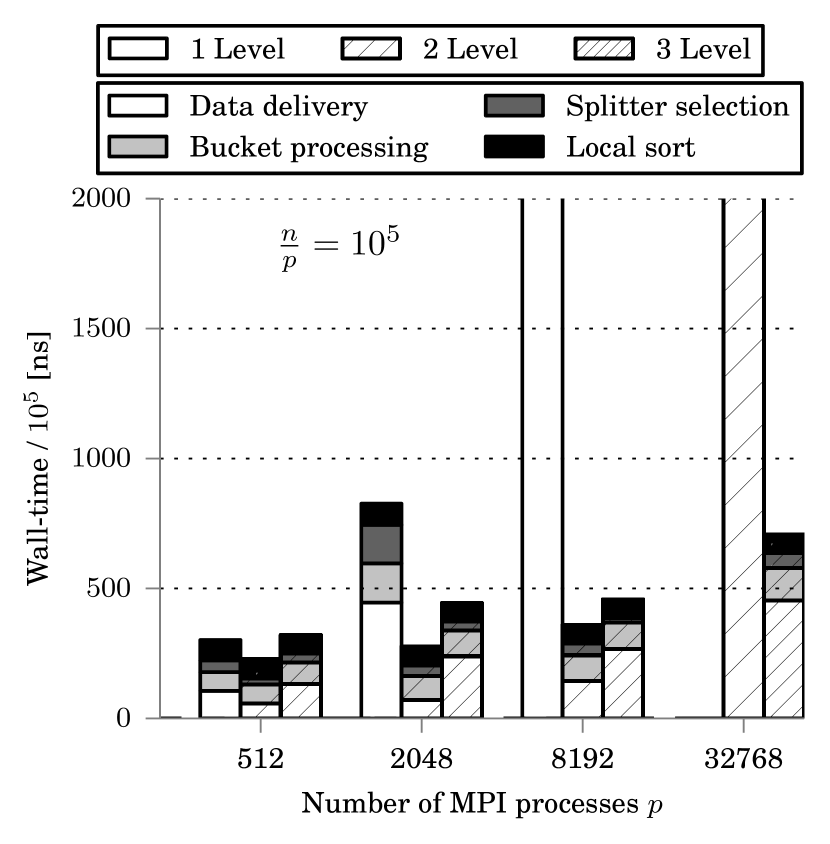
(a)

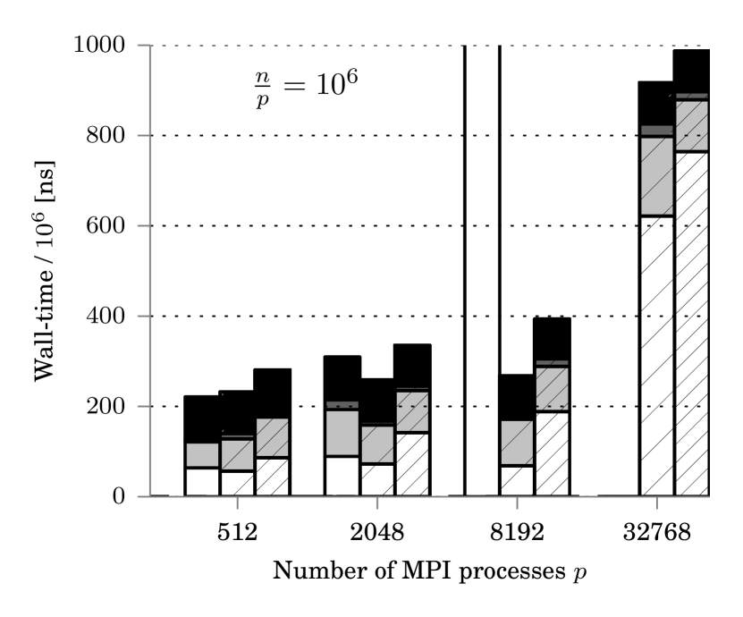
(b)

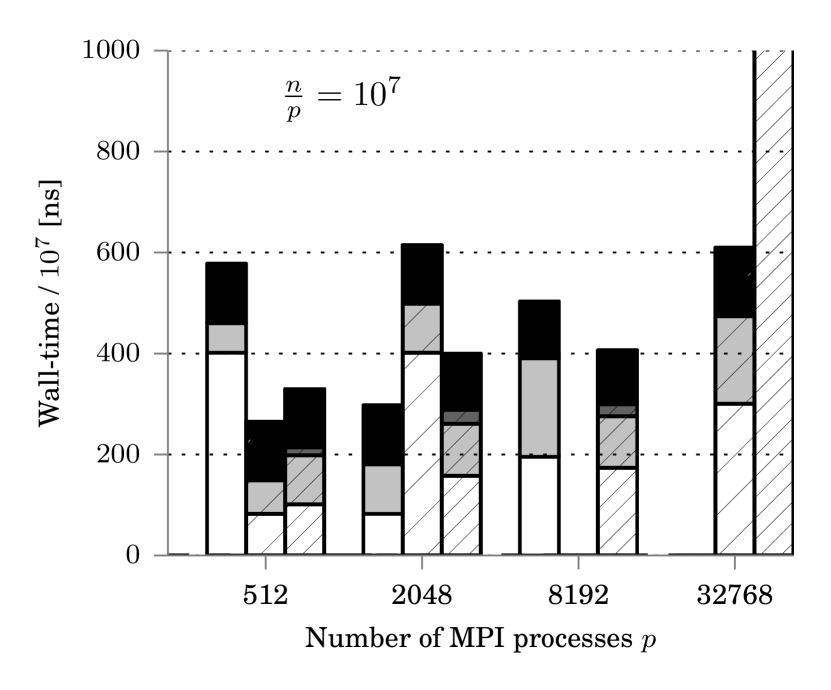
(c)

Figure 8: Weak scaling with $10^{5}$, $10^{6}$, and $10^{7}$ elements per MPI process of AMS-sort

The experimental setting of the weak scaling test is as follows: We benchmarked AMS-sort at $32$, $128$, $512$, and $2048$ nodes. Each node executed $16$ MPI processes. This results in $512$, $2048$, $8192$, and $32768$ MPI processes. The benchmark configuration for $2048$ nodes has been executed on four exclusively allocated islands. Table 1 shows the level configurations of our algorithm. AMS-sort, configured with more than one level, splits the remaining processes into groups with a size of $16$ MPI processes at the second to last level. Thereby, the last level communicates just node-internally. For the $3$-level AMS-sort, we split the MPI processes at the first level into $2^{\left\lceil\log(p)/2\right\rceil}$ groups. AMS-sort configured the splitter selection phase with an overpartitioning factor of $b=16$ and an oversampling factor of $a=1.6\>\log_{10}n$.

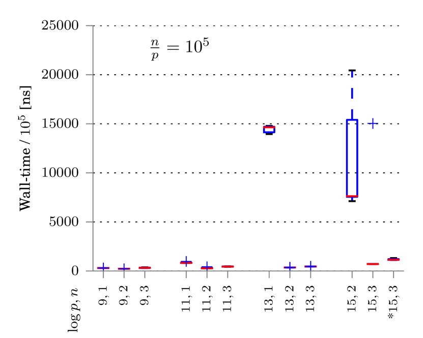
(a)

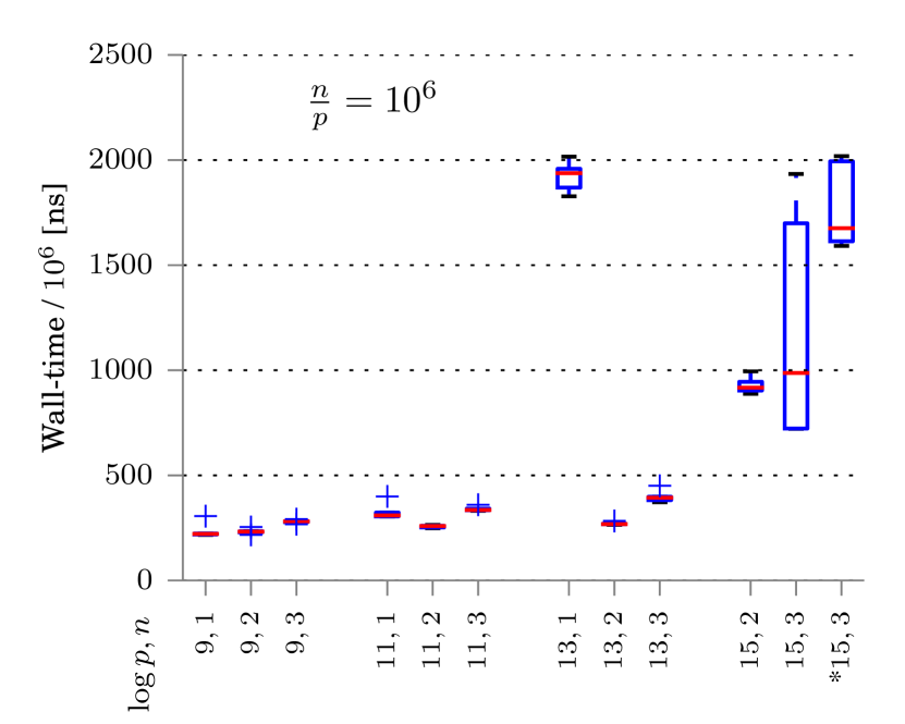
(b)

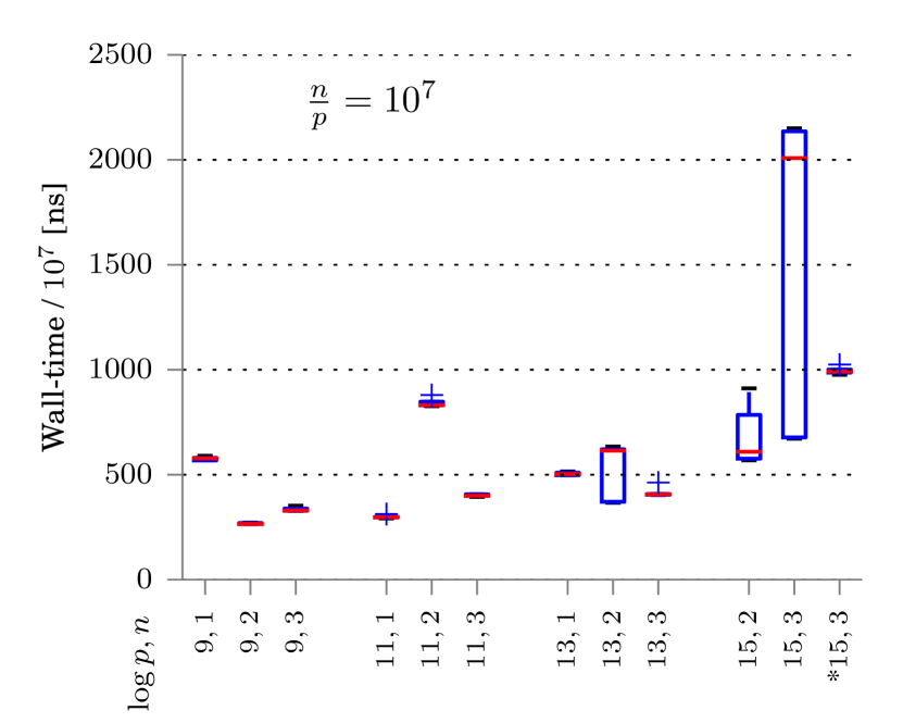
(c)

Figure 12: AMS-sort with $10^{5}$, $10^{6}$, and $10^{7}$ elements per MPI process

Figure 8 details the wall-time of AMS-sort up to three levels. For each wall-time, we show the proportion of time taken by each phase. The depicted wall-time is the median of five measurements. Figure 12 in the Appendix shows the distribution of the wall-times. Observe that AMS-sort is not limited by the splitter selection phase in all test cases. In most cases, AMS-sort with more than one level decreases the wall-time up to $8192$ MPI processes. Also, there is a speedup in the data delivery phase and no significant slowdown in the bucket processing phase due to cache effects. In these cases, the cost for partitioning the data and distributing more than once is compensated by the decreased number of startups. For the smaller volume of $10^{5}$ elements per MPI process, note that $3$-level AMS-sort is much faster than $2$-level AMS-sort in our experimental setup; the effect is reversed for more elements. Note that there is inter-island data delivery at the first and second level of $3$-level AMS-sort. The slowdown of sorting $10^{6}$ elements per MPI process with $3$-level AMS-sort compared to $2$-level AMS-sort is small. So we assume that the three level version becomes faster than the two level version executed at more than four islands. In that case, it is more reasonable to set the number of groups in the first level equal the amount of islands. This results in inter-island communication just within the first level.

Table 2 depicts the median wall-time of our weak scaling experiments of AMS-sort. Each entry is selected based on the level which performed best. For a fixed $p$, the wall-time increases almost linear with the amount of elements per MPI process. One exception is the wall-time for $8192$ nodes and $10^{7}$ elements. We were not able to measure the $2$-level AMS-sort as the MPI-implementation failed during this experiment. The wall-time increases by a small factor up to $8192$ MPI processes for increasing $p$. Executed with $32768$ MPI processes, AMS-sort is up to $3.5$ times slower compared to intra-island sorting, allocated at one whole island. The slowdown can be feasibly explained by the interconnect which connects islands among each other. The interconnect has an bandwidth ratio of $4:1$ compared to the intra-island interconnect.

Generally, for large $p$, the execution time fluctuates a lot (also see Figure 12). This fluctuation is almost exclusively within the all-to-all exchange. Further research has to show to what extent this is due to interference due to network traffic of other applications or suboptimal implementation of all-to-all data exchange. Both effects seem to be independent of the sorting algorithm however.

Figure 7 illustrates the slowdown of RLM-sort compared to AMS-sort. For each algorithm, we selected the number of levels with the best wall-time. Note that the slowdown of RLM-sort is higher than one in almost all test cases. The slowdown is significantly increased for small $n$ and large $p$. This observation matches with the isoefficiency function of RLM-sort which is a $\log^{2}p$ factor worse than the isoefficiency function of AMS-sort.

7.3 Comparison with Other Implementations

Comparisons to other systems are difficult, since it is not easy to simply download other people’s software and to get it to run on a large machine. Hence, we have to compare to the literature and the web. Our absolute running times for $n=10^{7}p$ are similar to those of observed in Solomonik and Kale [34] for $n=8\cdot 10^{6}\cdot p$ on a CrayXT 4 with up to $2^{15}$ PEs. This machine has somewhat slower PEs (2.1 GHz AMD Barcelona) but higher communication bandwidth per PE. No running times for smaller inputs are given. It is likely that there the advantage of multilevel algorithms such as ours becomes more visible. Still, we view it as likely that adapting their techniques for overlapping communication and sorting might be useful for our codes too.

A more recent experiment running on even more PEs is MP-sort [12]. MP-sort is a single-level multiway mergesort that implements local multiway merging by sorting from scratch. They run the same weak scaling test as us using up to 160 000 cores of a Cray XE6 (16 AMD Opteron cores $\times$ 2 processors $\times$ 5 000 nodes). This code is much slower than ours. For $n=10^{5}\cdot p$, and $p=2^{14}$ the code needs 20.45 seconds – 289 times more than ours for $p=2^{15}$. When going to $p=80\,000$ the running time of MP-sort goes up by another order of magnitude. At large $p$, MP-sort is hardly slower for larger inputs (however still about six times slower than AMS-sort). This is a clear indication that a single level algorithm does not scale for small inputs.

Different but also interesting is the Sort Benchmark which is quite established in the data base community (sortbenchmark.org). The closest category is Minute-Sort. The 2014 winner, Baidu-Sort (which uses the same algorithm as TritonSort [26]), sorts 7 TB of data (100 byte elements with 10 byte random keys) in 56.7s using 993 nodes with two 8-core processors (Intel Xeon E5-2450, 2.2 GHz) each ($p=15\,888$). Compared to our experiment at $n=10^{7}\cdot 2^{15}$, they use about half as many cores as us, and sort about 2.7 times more data. On the other hand, Baidu-Sort takes about 9.3 times longer than our 2-level algorithm. and we sort about 5 times more (8-byte) elements. Even disregarding that we also sort about 5 times more (8-byte) elements, this leaves us being about two times more efficient. This comparison is unfair to some extent since Minute-Sort requires the input to be read from disk and the result to be written to disk. However, the machine used by Baidu-Sort has 993$\times$8 hard disks. At a typical transfer rate of 150 MB/s this means that, in principle, it is possible to read and write more than 30 TB of data within the execution time. Hence, it seems that also for Baidu-Sort, the network was the major performance bottleneck.

8 Conclusion

We have shown how practical parallel sorting algorithms like multi-way mergesort and sample sort can be generalized so that they scale on massively parallel machines without incurring a large additional amount of communication volume. Already our prototypical implementation of AMS-sort shows very competitive performance that is probably the best by orders of magnitude for large $p$ and moderate $n$. For large $n$ it can compete with the best single-level algorithms.

Future work should include experiments on more PEs, a native shared-memory implementation of the node-local level, a full implementation of data delivery, faster implementation of overpartitioning, and, at least for large $n$, more overlapping of communication and computation. However, the major open problem seems to be better data exchange algorithms, possibly independently of the sorting algorithm.

Acknowledgments:

The authors gratefully acknowledge the Gauss Centre for Supercomputing e.V. (www.gauss-centre.eu) for funding this project by providing computing time on the GCS Supercomputer SuperMUC at Leibniz Supercomputing Centre (LRZ, www.lrz.de) Special thanks go to SAP AG, Ingo Mueller, and Sebastian Schlag for making their 1-factor algorithm [29] available. Additionally, we would like to thank Christian Siebert for valuable discussions.

Appendix A Randomized Data Delivery

Figure 9: Exchange schema with the advanced randomized algorithm.

Our advanced randomized data delivery algorithm is asymptotically more efficient than the simple one described in Section 4.3 and it may be simpler to implement than the deterministic one from Section 4.3.1 since no parallel merging operation is needed. Compared to the simple algorithm, the algorithm adds more randomization and invests some additional communication. The idea is to break large pieces into several smaller pieces. A piece whose size $x$ exceeds a limit $s$ is broken into $\left\lfloor x/s\right\rfloor$ pieces of size $s$ and one piece of size $x\bmod s$. We set $s:=an/rp$ to be $a$ times the average piece size $n/rp$ where $a$ is a tuning parameter to be chosen later. The resulting small pieces (size below $s$) stay where they are and the random permutation of the PE numbers takes care of their random placement. The large pieces are delegated to another (random) PE using a further random permutation. This is achieved by enumerating them globally over all parts using a prefix sum. Suppose there are $K$ large pieces, then we use a pseudorandom permutation $\pi:0..K-1\rightarrow 0..K-1$ to delegate piece $i$ to PE $1+\pi(i)\bmod p$. Note that this assignment only entails to tell PE $j$ about the origin of this piece and its target group – there is no need to move the actual elements at this point. In Figure 9, we denote the delegation tuples with origin PE $p$ and target group $r$ as $(r,p)$. Next, for each part, a PE reorders its small pieces and delegated large pieces randomly (of course without choosing the intra-piece sorting). Only then, a prefix sum is used to enumerate the elements in each part. The ranges of numbers assigned to the pieces are then communicated back to the PEs actually holding the data and we continue as in the basic approach – computing target PEs based on the received ranges of numbers.

Lemma A.12.

The two stage approach needs time $\mathcal{O}(\alpha\log p+r\beta)+2\mathrm{Exch}(p,\mathcal{O}(r/a),\left\lceil r/a\right\rceil)$ to assign data to target PEs.

Proof A.13.

Each PE will produce at most $\frac{n/p}{s}=\frac{n/p}{an/rp}=r/a$ large pieces. Overall, there will be at most $\frac{n}{s}=\frac{n}{an/rp}=pr/a$ large pieces. The random mapping will delegate at most $\left\lceil r/a\right\rceil$ of these messages to each PE with high probability. Since each delegation and notification message has constant size, $2\mathrm{Exch}(p,\mathcal{O}(r/a),\left\lceil r/a\right\rceil)$ accounts for the resulting communication costs. All involved prefix sums are vector valued prefix sum with vector length $r$ and can thus be implemented to run in time $\mathcal{O}(\alpha\log p+r\beta)$. This term also covers the local computations.

Lemma A.14.

No PE sends more than $2r(1+1/a)$ messages during the main data exchange of one phase of RLM-sort. Moreover, the total number of messages for a single part is at most $p(1+1/r+1/a)$.

Proof A.15.

As shown above, each PE produces at most $r(1+1/a)$ pieces, each of which may be split into at most two messages. For each part, there are at most $p$ small pieces and $\frac{n/r}{an/rp}=p/a$ large pieces. At most $p/r-1<p/r$ pieces can be split because their assigned range of element numbers intersects the ranges of responsibility of two PEs. Overall, we get $p(1+1/r+1/a)$ messages per part.

Lemma A.16.

Assuming that our pseudorandom permutations behave like truly random permutations, with probability $1-\mathcal{O}(1/p)$, no PE receives more than $1+2r(1+1/a)$ messages during one phase of RLM-sort for some value of $a\in\Theta(\sqrt{r/\log p})$.

Proof A.17.

Let $m\leq p(1+1/a)$ denote the number of pieces generated for part $x$. It suffices to prove that the probability that any of the PEs responsible for it receives more than $1+2mr/p\leq 2r(1+1/a)$ messages is at most $1/rp$ for an appropriate constant. We now abstract from the actual implementation of data assignment by observing that the net effect of our randomization is to produce a random permutation of the pieces involved in each part. In this abstraction, the “bad” event can only occur if the permutation produces $2mr/p$ consecutive pieces of total size at most $n/p$. More formally, let $X_{1}$,…,$X_{m}$ denote the piece sizes. The $X_{i}$ are random variables with range $[0,\frac{an}{rp}]$ and $\sum_{i}X_{i}=n/r$. The randomness stems from the random permutation determining the ordering. Unfortunately, the $X_{i}$ are not independent of each other. However, they are negatively associated [11], i.e., if one variable is large, then a different variable tends to be smaller. In this situation, Chernoff-Hoeffding bounds for the probability that a sum deviates from its expectation still apply. Now, for a fixed $j$, consider $X\mbox{\rm:= }\sum_{j\leq i<j+2mr/p}X_{i}$. It suffices to show that – in that case, the probability that the bad event occurs for some $j$ is at most $1/rp$. We have ${\mathbf{E}}[X]=2n/p$ which differs by $t\mbox{\rm:= }n/p$ from the bound marking a bad event. Hoeffding’s inequality then assures that the probability of the bad event is at most

$$\leq 2e^{-\frac{2t^{2}}{\frac{2mr}{r}\cdot\left(\frac{an}{rp}\right)^{2}}}=2e^{-\frac{pr}{ma^{2}}}\leq 2e^{-\frac{pr}{a^{2}+1}}\enspace.$$

This should be smaller than $1/rp$. Solving the resulting relation for $a$ yields

$$a\leq\frac{1}{2}\left(\sqrt{1+\frac{r}{\ln\frac{rp}{2}}}-1\right)\enspace.$$

Note that Lemma A.16 implies that with high probability both the number of sent and received messages during data exchange will be close to $2r$ and the number of message startups for delegating pieces (see Lemma A.12) will be $o(r)$. Hence, we have shown that handling worst case inputs by our algorithm adds only lower order cost terms compared to the simple variant (plain prefix sums without any randomization) on average case inputs. In contrast, applying the simple approach to worst case inputs directly, completely ruins performance.

We summarize the result in the following theorem:

Theorem A.18.

Data delivery of $r\times p$ pieces to $r$ parts can be implemented to run in time

$$\smash{\mathrm{Exch}\hbox to0.0pt{\hss\raisebox{-3.0pt}{$\widetilde{\phantom{iih}}$}\hskip 3.8pt}}(p,\tfrac{n}{p},2r)$$

with high probability.

Appendix B Pseudorandom Permutations

During redistribution of data, we will randomize the rearrangement to avoid bad cases. For this, we select a pseudo-random permutation, which can be constructed, e.g., by composing three to four Feistel permutations [23, 10]. We adapt the description from [10] to our purposes.

Assume we want to compute a permutation $\pi:0..n-1\rightarrow 0..n-1$. Assume for now that $n$ is a square so that we can represent a number $i$ as a pair $(a,b)$ with $i=a+b\sqrt{n}$. Our permutations are constructed from Feistel permutations, i.e., permutations of the form $\pi_{f}((a,b))=(b,a+f(b)\bmod\sqrt{n})$ for some pseudorandom mapping $f:0..\sqrt{n}-1\rightarrow 0..\sqrt{n}-1$. $f$ can be any hash function that behaves reasonably similar to a random function in practice. It is known that a permutation $\pi(x)=\pi_{f}(\pi_{g}(\pi_{h}(\pi_{l}(x))))$ build by chaining four Feistel permutations is “pseudorandom” in a sense useful for cryptography. The same holds if the innermost and outermost permutation is replaced by an even simpler permutation [25]. In [10], we used just two stages of Feistel-Permutations.

A permutation $\pi^{\prime}$ on $0..\left\lceil\sqrt{n}\right\rceil^{2}-1$ can be transformed to a permutation $\pi$ on $0..n-1$ by iteratively applying $\pi^{\prime}$ until a value below $n$ is obtained. Since $\pi^{\prime}$ is a permutation, this process must eventually terminate. If $\pi^{\prime}$ is random, the expected number of iterations is close to $1$ and it is unlikely that more than three iterations are necessary

Since the description of $\pi$ requires very little state, we can replicate this state over all PEs.

Appendix C Accelerating Bucket Grouping

The first observation for improving the binary search algorithm from Section 6 is that a PE-group size can take only $\mathcal{O}((br)^{2})$ different values since it is defined by a range of buckets. We can modify the binary search in such a way that it operates not over all conceivable group sizes but only over those corresponding to ranges of buckets. When a scanning step succeeds, we can safely reduce the upper bound for the binary search to the largest PE-group actually used. On the other hand, when a scanning step fails, we can increase the lower bound: during the scan, whenever we finish a PE-group of size $x$ because the next bucket of size $y$ does not fit (i.e., $x+y>L$), we compute $z=x+y$. The minimum over all observed $z$-values is the new lower bound. This is safe, since a value of the scanning bound $L$ less then $z$ will reproduce the same failed partition. This already yields an algorithm running in time $\mathcal{O}(br\log(br)^{2})=\mathcal{O}(br\log(br))$.

The second observation is only values for $L$ in the range $\left\lceil n/r-1\right\rceil..(1+\mathcal{O}(1/b))n/r$ are relevant (see Lemma 6.6). Only $\mathcal{O}(br)$ bucket ranges will have a total size in this range. To see this, consider any particular starting bucket for a bucket range. Searching from there to the right for range end points, we can skip all end buckets where the total size is below $n/r$. We can stop as soon as the total size leaves the relevant range. Since buckets have average size $\mathcal{O}(n/b)$, only a constant number of end points will be in the relevant range on the average. Overall, we get $\mathcal{O}(br)\cdot\mathcal{O}(1)=\mathcal{O}(br)$ relevant bucket ranges. Using this for initializing the binary search, saves a factor about two for the sequential algorithm.

Using all $p$ available PEs, we can do even better: in each iteration, we split the remaining range for $L$ evenly into $p+1$ subranges. Each PE tries one subrange end point for scanning and uses the first observation to round up or down to an actually occurring size of a bucket range. Using a reduction we find the largest $L$-value $L_{\min}$ for a failed scan and the smallest $L$ value $L_{\max}$ for a successful scan. When $L_{\max}=L_{\min}$ we have found the optimal value for $L$. Otherwise, we continue with the range $L_{\max}..L_{\min}$. Since the bucket range sizes in the feasible region are fairly uniformly distributed, the number of iterations will be $\log_{p+1}\mathcal{O}(br)$. Since $p\geq r$, this is $\mathcal{O}(1)$ if $b$ is polynomial in $r$. Indeed, one or two iterations are likely to succeed in all reasonable cases.

Appendix D Tie Breaking for Key Comparisons

Conceptually, we assign the key $(x,i,j)$ to an element with key $x$, stored on PE $i$ at position $j$ of the input array. Using lexicographic ordering makes the keys unique. For a practical implementation, it is important not to do this explicitly for every element. We explain how this can be done for AMS-sort. First note, that in AMS-sort there is no need to do tie breaking across levels or for the final local sorting. Sample sorting and splitter determination can afford to do tie breaking explicitly, since these steps are more latency bound. For partitioning, we can use a version of super scalar sample sort, that also produces a bucket for elements equal to the splitter. This takes only one additional comparison [5] per element. Only if an input element $x$ ends up in an equality bucket we need to perform the lexicographic comparison. Note that at this point, the PE number for $x$ and its input position are already present in registers anyway.

Appendix E Additional Experimental Data

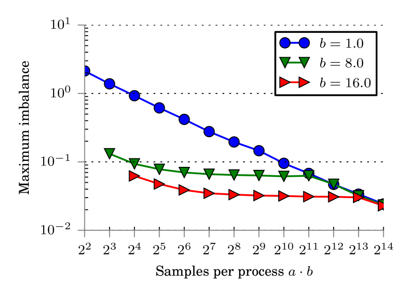
Figure 10: Maximum imbalance among groups of AMS-sort sorted sequences

Figure 11: Wall-time of AMS-sort for various values of $a$ and $b$

The overpartitioning factor $b$ influences the wall-time of AMS-sort. It has an effect on the splitter selection phase itself but also an implicit impact on all other phases. To investigate this impact, we executed AMS-sort for various values of $b$ with $512$ MPI processes and $10^{5}$ elements each. Figure 11 shows how the wall-time of AMS-sort depends on the number of samples per process $a\cdot b$. Depending on the oversampling factor $a$, the wall-time firstly decreases as the maximum imbalance decreases. This leads to faster data delivery, bucket processing, and splitter selection phases. However, the wall-time increases for large $a$ as the additional cost of the splitter selection phase dominates. On the one hand, AMS-sort performs best for an oversampling factor of $1$ and an overpartitioning factor of $64$. On the other hand, Figure 10 illustrates that the maximum imbalance is significantly higher for slightly slower AMS-sort algorithms, configured with $b>1$.

References

- [1] M. Axtmann, T. Bingmann, P. Sanders, and C. Schulz. Practical Massively Parallel Sorting – Basic Algorithmic Ideas. Preprint arXiv:1410.6754v1, Oct. 2014.
- [2] V. Bala, J. Bruck, R. Cypher, P. Elustondo, A. Ho, C. Ho, S. Kipnis, and M. Snir. CCL: A portable and tunable collective communication library for scalable parallel computers. IEEE Transactions on Parallel and Distributed Systems, 6(2):154–164, 1995.
- [3] K. E. Batcher. Sorting networks and their applications. In AFIPS Spring Joint Computing Conference, pages 307–314, 1968.
- [4] A. Bäumker, W. Dittrich, and F. Meyer auf der Heide. Truly efficient parallel algorithms: -optimal multisearch for an extension of the BSP model. In Algorithms — ESA’95, pages 17–30. Springer, 1995.
- [5] T. Bingmann, A. Eberle, and P. Sanders. Engineering parallel string sorting. Preprint arXiv:1403.2056, 2014.
- [6] G. E. Blelloch et al. A comparison of sorting algorithms for the connection machine CM-2. In 3rd Symposium on Parallel Algorithms and Architectures, pages 3–16, 1991.
- [7] S. Borkar. Exascale computing – a fact or a fiction? Keynote presentation at IPDPS 2013, Boston, May 2013.
- [8] G. S. Brodal, R. Fagerberg, and K. Vinther. Engineering a cache-oblivious sorting algorithm. In 6th Workshop on Algorithm Engineering and Experiments, 2004.
- [9] R. Cole. Parallel merge sort. SIAM Journal on Computing, 17(4):770–785, 1988.
- [10] R. Dementiev, P. Sanders, D. Schultes, and J. Sibeyn. Engineering an external memory minimum spanning tree algorithm. In IFIP TCS, pages 195–208, Toulouse, 2004.
- [11] D. Dubhashi, V. Priebe, and D. Ranjan. Negative dependence through the FKG inequality. Research Report MPI-I-96-1-020, Max-Planck-Institut für Informatik, Im Stadtwald, D-66123 Saarbrücken, Germany, Aug. 1996.
- [12] Y. Feng, M. Straka, T. di Matteo, and R. Croft. MP-sort: Sorting at scale on blue waters. https://www.writelatex.com/read/sttmdgqthvyv accessed Jan 17, 2015, 2014.
- [13] A. Gerbessiotis and L. Valiant. Direct bulk-synchronous parallel algorithms. Journal of Parallel and Distributed Computing, 22(2):251–267, 1994.
- [14] M. T. Goodrich. Communication-efficient parallel sorting. SIAM Journal on Computing, 29(2):416–432, 1999.
- [15] T. Hagerup and C. Rüb. Optimal merging and sorting on the EREW-PRAM. Information Processing Letters, 33:181–185, 1989.
- [16] C. A. R. Hoare. Algorithm 65 (find). Communication of the ACM, 4(7):321–322, 1961.
- [17] L. Hübschle-Schneider, I. Müller, and P. Sanders. Communication efficient algorithms for top-k selection problems. submitted for SPAA 2015, 2015.
- [18] M. Ikkert, T. Kieritz, and P. Sanders. Parallele Algorithmen. course notes, October 2009.
- [19] J. Jájá. An Introduction to Parallel Algorithms. Addison Wesley, 1992.
- [20] D. E. Knuth. The Art of Computer Programming—Sorting and Searching. Addison Wesley, 1998.
- [21] V. Kumar, A. Grama, A. Gupta, and G. Karypis. Introduction to Parallel Computing. Design and Analysis of Algorithms. Benjamin/Cummings, 1994.
- [22] H. Li and K. C. Sevcik. Parallel sorting by overpartitioning. In ACM Symposium on Parallel Architectures and Algorithms, pages 46–56, Cape May, New Jersey, 1994.
- [23] M. Luby and C. Rackoff. How to construct pseudorandom permutations from pseudorandom functions. SIAM Journal on Computing, 17(2):373–386, Apr. 1988.
- [24] K. Mehlhorn and P. Sanders. Algorithms and Data Structures — The Basic Toolbox. Springer, 2008.
- [25] M. Naor and O. Reingold. On the construction of pseudorandom permutations: Luby-Rackoff revisited. Journal of Cryptology: the journal of the International Association for Cryptologic Research, 12(1):29–66, 1999.
- [26] A. Rasmussen, G. Porter, M. Conley, H. V. Madhyastha, R. N. Mysore, A. Pucher, and A. Vahdat. Tritonsort: A balanced large-scale sorting system. In NSDI, 2011.
- [27] P. Sanders. Fast priority queues for cached memory. ACM Journal of Experimental Algorithmics, 5, 2000.
- [28] P. Sanders. Course on Parallel Algorithms, lecture notes, 2008. http://algo2.iti.kit.edu/sanders/courses/paralg08/.
- [29] P. Sanders, S. Schlag, and I. Müller. Communication efficient algorithms for fundamental big data problems. In IEEE Int. Conf. on Big Data, 2013.
- [30] P. Sanders, J. Speck, and J. L. Träff. Two-tree algorithms for full bandwidth broadcast, reduction and scan. Parallel Computing, 35(12):581–594, 2009.
- [31] P. Sanders and J. L. Träff. The factor algorithm for regular all-to-all communication on clusters of SMP nodes. In 8th Euro-Par, number 2400, pages 799–803. Springer ©, 2002.
- [32] P. Sanders and S. Winkel. Super scalar sample sort. In 12th European Symposium on Algorithms, volume 3221 of LNCS, pages 784–796. Springer, 2004.
- [33] J. Singler, P. Sanders, and F. Putze. MCSTL: The multi-core standard template library. In 13th Euro-Par, volume 4641 of LNCS, pages 682–694. Springer, 2007.
- [34] E. Solomonik and L. Kale. Highly scalable parallel sorting. In IEEE International Symposium on Parallel Distributed Processing (IPDPS), pages 1–12, April 2010.
- [35] L. Valiant. A bridging model for parallel computation. Communications of the ACM, 33(8):103–111, 1994.
- [36] P. J. Varman et al. Merging multiple lists on hierarchical-memory multiprocessors. J. Par. & Distr. Comp., 12(2):171–177, 1991.