Nodal domains in the square—the Neumann case

Abstract.

Å. Pleijel has proved that in the case of the Laplacian on the square with Neumann condition, the equality in the Courant nodal theorem (Courant sharp situation) can only be true for a finite number of eigenvalues. We identify five Courant sharp eigenvalues for the Neumann Laplacian in the square, and prove that there are no other cases.

1. Introduction

For an eigenfunction $\Psi_{n}$ corresponding to the $n$-th eigenvalue $\lambda_{n}$ (counted with multiplicity) of the Laplace operator in a bounded regular domain $\Omega$, we denote by $\mu(\Psi_{n})$ the number of nodal domains of $\Psi_{n}$. A famous result by Courant (see [4]) states that $\mu(\Psi_{n})\leq n$. If $\mu(\Psi_{n})=n$, then we say that the eigenpair $(\lambda_{n},\Psi_{n})$ (or just the eigenvalue $\lambda_{n}$) is Courant sharp. It is proved in [15, 17] that, for general planar domains, and with Dirichlet or Neumann boundary conditions, the Courant sharp situation occurs for a finite number of eigenvalues only. Note that in the case of Neumann the additional assumption that the boundary is piecewise analytic should be imposed due the use of a theorem by Toth–Zelditch [20] counting the number of nodal domains whose closure is touching the boundary.

In the recent years, the question of determining the Courant sharp cases reappears in connection with the determination of minimal spectral partitions in the work of Helffer–Hoffmann-Ostenhof–Terracini [8]. The Courant sharp situation was analyzed there in the case of the irrational rectangle and in the case of the disk for Dirichlet boundary condition. The case of anisotropic (irrational) tori is solved in [7].

Recently the Courant sharp cases were identified in the cases of $\Omega$ being a square with Dirichlet boundary conditions imposed [15, 1], and $\Omega$ being the two-sphere [2]. Here, our aim is to do the same detailed analysis in the case of $\Omega$ being a square with Neumann boundary conditions.

We let $\Omega=\{(x,y)\in\mathbb{R}^{2}~{}|~{}0<x<\pi,\ 0<y<\pi\}$ and denote by $L$ the self-adjoint Neumann Laplacian in $L^{2}(\Omega)$. This operator has eigenvalues

$$0=\lambda_{1}<\lambda_{2}\leq\cdots\leq\lambda_{n}\leq\cdots,$$

generated by the set $\{p^{2}+q^{2}~{}|~{}p,q\in\mathbb{N}\cup\{0\}\}$. A basis for the eigenspace corresponding to the eigenvalue $\lambda=p^{2}+q^{2}$ is given by

$$\{\cos px\cos qy~{}|~{}p,q\in\mathbb{N}\cup\{0\},\ p^{2}+q^{2}=\lambda\}.$$

Å. Pleijel was in particular referring to figures appearing in the book of Pockels [16] (and partially reproduced in [5]) like in the Figure 1.

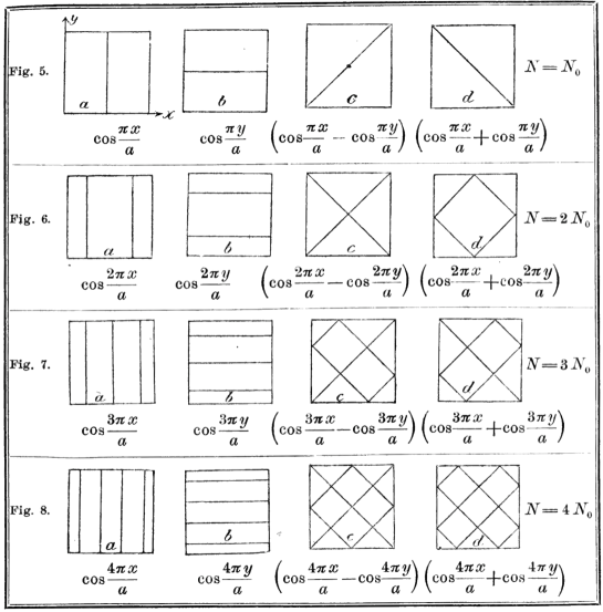
Figure 1. Nodal patterns for the Neumann eigenfunctions in the square $(0,1)^{2}$ in the book of Pockels (1891).

Theorem 1.1.

There exists a Courant sharp eigenpair $(\lambda_{n},\Psi_{n})$ if and only if $n\in\{1,2,4,5,9\}$.

The Courant sharpness of eigenvalues $\lambda_{1}$, $\lambda_{2}$ and $\lambda_{5}$ follows from Lemma 4.2 and the Courant sharpness of $\lambda_{4}$ and $\lambda_{9}$ follows from Lemma 4.4. These cases are illustrated in Figure 2. They correspond to the zero sets of the following eigenfunctions:

• $n=1$ : $(x,y)\mapsto 1$ ;

• $n=2$ : $(x,y)\mapsto\cos\theta\cos x+\sin\theta\cos y\,$ (with $\theta=1$ in Figure 2);

• $n=4$ : $(x,y)\mapsto\cos x\cos y\,$;

• $n=5$ : $(x,y)\mapsto\cos 2x+\cos 2y\,$;

• $n=9$ : $(x,y)\mapsto\cos 2x\cos 2y\,$.

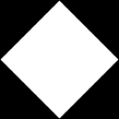
Figure 2. The figure shows the nodal sets in the five Courant sharp cases. From left to right, $n=1$, $n=2$, $n=4$, $n=5$, $n=9$. In each example the black and white areas represent nodal domains where the function has different sign.

The proof of Theorem 1.1 is divided into several lemmas and propositions. Although following the general scheme proposed by Å. Pleijel [15] and completed in [1] for the Dirichlet case, the realization of the program in the case of Neumann is more difficult and finally involves a combination of arguments present in [15], [18], [13], [14], [8], [7] and [1].

First we reduce to a finite number of possible Courant sharp cases in Section 2. In Section 3 we use different symmetry arguments. In Section 4, we consider two families of eigenfunctions corresponding to $\lambda=p^{2}$ and $\lambda=2p^{2}$ for which a complete description is easy.

Section 5 gives the general approach for the analysis of the critical points and the boundary points together with a rough localization of the zero set initiated by A. Stern: the chessboard localization. The rest of the cases, which needs a separate treatment, are taken care of in Sections 6 and 7. In Section 8 we indicate how one can improve the estimates, if striving for optimal results. Finally, in Section 9 we give a list of all eigenvalues together with a reference to the lemma in which they are treated. We conclude by a short discussion on open problems.

Proposition 2.1 below reduces our study to a finite number of eigenvalues. We provide animations showing the nodal domains in all finite cases studied where the eigenspace is two-dimensional.

2. Necessary conditions for Courant sharpness and first reductions

Given an eigenfunction $\Psi$, we introduce the subset $\Omega^{\text{inn}}\subseteq\Omega$ as the union of nodal domains of $\Psi$ that do not touch the boundary of $\Omega$, except at isolated points. We also introduce $\Omega^{\text{out}}\subseteq\Omega$ as the union of nodal domains of $\Psi$ not belonging to $\Omega^{\text{inn}}$. We also denote by $\mu^{\text{inn}}(\Psi)$ and $\mu^{\text{out}}(\Psi)$ the number of nodal domains of $\Psi$ restricted to $\Omega^{\text{inn}}$ and $\Omega^{\text{out}}$, respectively. It is clear that

$$\mu(\Psi)=\mu^{\text{inn}}(\Psi)+\mu^{\text{out}}(\Psi).$$

From [15] we know that if $(\lambda_{n},\Psi_{n})$ is an eigenpair of $L$ then

$$\mu^{\text{out}}(\Psi_{n})\leq 4\sqrt{\lambda_{n}}.$$ (2.1)

Moreover, we can write $\Omega^{\text{inn}}=\bigcup_{i}\Omega^{\text{inn}}_{i}$ as a finite union of pairwise disjoint nodal domains for $\Psi_{n}$. The Faber–Krahn inequality [6, 10] for each inner nodal domain $\Omega^{\text{inn}}_{i}$ says

$$\frac{1}{\lambda_{n}}\leq\frac{\bigl{|}\Omega^{\text{inn}}_{i}\bigr{|}}{\pi j_{0,1}^{2}},$$ (2.2)

where $\bigl{|}\Omega^{\text{inn}}_{i}\bigr{|}$ denotes the area of $\Omega^{\text{inn}}_{i}$ and $j_{0,1}$ the first positive zero of the Bessel function $J_{0}$. Summing, we get

$$\mu^{\text{inn}}(\Omega)\leq\,\frac{\bigl{|}\Omega^{\text{inn}}\bigr{|}}{\pi j_{0,1}^{2}}\lambda_{n}.$$ (2.3)

Proposition 2.1.

Assume that $(\lambda_{n},\Psi_{n})$ is a Courant sharp eigenpair. Then $n\leq 208$.

Proof.

Let $N(\lambda)$ denote the number of eigenvalues strictly less than $\lambda$, counting multiplicity. The Weyl law [21] says that $N(\lambda)\sim\frac{\pi}{4}\lambda$ but we need the following universal lower bound for the Neumann problem in the square obtained by direct counting (see [15] for the Dirichlet case with the correction mentioned in [1]):

$$N(\lambda)>\frac{\pi}{4}\lambda.$$ (2.4)

Assume that $(\lambda_{n},\Psi_{n})$ is a Courant sharp eigenpair. The theorem of Courant implies that $\lambda_{n}>\lambda_{n-1}$ and $N(\lambda_{n})=n-1$. Inserting this into (2.4) gives us

$$\lambda_{n}<\frac{4}{\pi}(n-1).$$

Combining this with (2.1) and (2.3), and the estimate $|\Omega^{\text{inn}}|\leq|\Omega|=\pi^{2}$,

$$n=\mu(\Psi_{n})\leq\frac{\bigl{|}\Omega^{\text{inn}}\bigr{|}}{\pi j_{0,1}^{2}}\lambda_{n}+4\sqrt{\lambda_{n}}<\frac{4}{j_{0,1}^{2}}(n-1)+\frac{8}{\sqrt{\pi}}\sqrt{n-1}.$$

This inequality is false if $n\geq 209$. ∎

Depending on the cases, we can consider many variants of the intermediate steps in the proof of Proposition 2.1 and introduce small useful improvements which can be used directly.

Lemma 2.2.

Assume that $(\lambda_{n},\Psi_{n})$ is an eigenpair of $L$. Then

$$\mu(\Psi_{n})\leq\frac{\bigl{|}\Omega^{\text{inn}}\bigr{|}}{\pi j_{0,1}^{2}}\lambda_{n}+4\lfloor\sqrt{\lambda_{n}}\rfloor\,.$$ (2.5)

Proof.

This follows immediately from (2.1) and (2.3) together with the fact that $\mu^{\text{out}}(\Psi_{n})$ must be an integer. ∎

For $n\geq 1$, we denote by $P_{n}:=\max\{p~{}|~{}p^{2}+q^{2}=\lambda_{n},\ p,q\in\mathbb{N}\cup\{0\}\}$.

Lemma 2.3.

Assume that $(\lambda_{n},\Psi_{n})$ is an eigenpair of $L$. Then

$$\mu(\Psi_{n})\leq\frac{\pi}{j_{0,1}^{2}}\lambda_{n}+\max{(4P_{n},1)}\,.$$

Proof.

We observe that $\mu^{\text{out}}(\Psi_{n})\leq\max{(4P_{n},1)}$. Hence,

$$\mu(\Psi_{n})=\mu^{\text{inn}}(\Psi_{n})+\mu^{\text{out}}(\Psi_{n})\leq\frac{\pi}{j_{0,1}^{2}}\lambda_{n}+\max{(4P_{n},1)}.\qed$$

Corollary 2.4.

The eigenvalues $\lambda_{n}$, where $n$ is one of 86, 95–96, 99–100, 103–104, 113, 118–119, 120–121, 128–142, 147–208, are not Courant sharp.

Proof.

Assume that $n$ is such that $\lambda_{n-1}<\lambda_{n}$. Then, a numerical calculation shows that

$$\frac{\pi}{j_{0,1}^{2}}\lambda_{n}+4P_{n}<n$$

for the $n$ mentioned in the statement. ∎

3. Reduction by symmetry

3.1. Preliminaries

Symmetry arguments will play an important role in the analysis of the Courant sharp situation. These ideas appear already in the case of the harmonic oscillator and the sphere in contributions by J. Leydold [13, 14].

We introduce the notation

$$\Phi_{p,q}^{\theta}(x,y)=\cos\theta\cos px\cos qy+\sin\theta\cos qx\cos py.$$ (3.1)

We will often write just $\Phi(x,y)$ or $\Phi_{p,q}(x,y)$. For eigenvalues of $L$ of multiplicity two, the family $\Phi_{p,q}^{\theta}(x,y)$, $0\leq\theta<\pi$ will give all possible eigenfunctions (up to multiplication by a non zero constant). Moreover, the basis of our arguments are the rich symmetry of the trigonometric functions. The role of the antipodal map in the case of the sphere is now replaced in the case of the sphere by the map:

$$(x,y)\mapsto(\pi-x,\pi-y)\,.$$

A finer analysis will involve the finite group generated by the maps $(x,y)\mapsto(\pi-x,y)$ and $(x,y)\mapsto(x,\pi-y)$.

3.2. Odd eigenvalues

We introduce $L^{\text{ARot}}$, the Neumann Laplacian restricted to the antisymmetric space

$$\mathcal{H}^{\text{ARot}}=\{\psi~{}|~{}\psi(\pi-x,\pi-y)=-\psi(x,y)\}\,.$$

The spectrum of this Laplacian is given by $p^{2}+q^{2}$ with $p+q$ odd. We denote by $(\lambda_{n}^{\text{ARot}})_{n=1}^{+\infty}$ the sequence of eigenvalues of $L^{\text{ARot}}$, counted with multiplicity. Then each odd $\lambda_{n}$ equals $\lambda_{m}^{\text{ARot}}$ for some $m$. The next lemma is an adaptation of Courant’s theorem in this subspace.

Lemma 3.1.

Assume that $(\lambda_{n},\Psi_{n})$ is an eigenpair of $L$, with $\lambda_{n}$ odd, and let $m$ be such that $\lambda_{n}=\lambda_{m}^{\text{ARot}}$. Then $\mu(\Psi_{n})$ is even, and

$$\mu(\Psi_{n})\leq 2m\,.$$

The proof is inspired by a proof of Leydold [14] (used in the case of the sphere). See also Leydold [13] and Bérard-Helffer [3] for the case of the harmonic oscillator.

Proof.

By assumption we have

$$\Psi_{n}(\pi-x,\pi-y)=-\Psi_{n}(x,y)\,.$$

This implies that $\mu(\Psi_{n})$ is even and that the family of nodal domains is the disjoint union of $r$ pairs, each pair consisting of two disjoint open sets exchanged by $(x,y)\mapsto(\pi-x,\pi-y)$. Restricting $\Psi_{n}$ to each pair, we obtain an $r$-dimensional antisymmetric space whose energy is bounded by $\lambda_{n}$. Hence $\lambda_{n}\geq\lambda_{r}^{\text{ARot}}$ by the min-max principle and $m\geq r$. Thus $\mu(\Psi_{n})=2r\leq 2m$. ∎

Corollary 3.2.

The eigenvalues $\lambda_{7}=\lambda_{8}$, $\lambda_{23}=\lambda_{24}=\lambda_{25}=\lambda_{26}$, $\lambda_{29}=\lambda_{30}$, $\lambda_{36}=\lambda_{37}$, $\lambda_{40}=\lambda_{41}$, $\lambda_{51}=\lambda_{52}$, $\lambda_{55}=\lambda_{56}$, $\lambda_{59}=\lambda_{60}=\lambda_{61}=\lambda_{62}$, $\lambda_{72}=\lambda_{73}$, $\lambda_{76}=\lambda_{77}=\lambda_{78}=\lambda_{79}$, $\lambda_{91}=\lambda_{92}$, $\lambda_{97}=\lambda_{98}$, $\lambda_{99}=\lambda_{100}$, $\lambda_{103}=\lambda_{104}$, $\lambda_{109}=\lambda_{110}=\lambda_{111}=\lambda_{112}$, $\lambda_{120}=\lambda_{121}$, $\lambda_{124}=\lambda_{125}=\lambda_{126}=\lambda_{127}$, $\lambda_{132}=\lambda_{133}$, $\lambda_{143}=\lambda_{144}=\lambda_{145}=\lambda_{146}$, $\lambda_{151}=\lambda_{152}$, $\lambda_{157}=\lambda_{158}$, $\lambda_{159}=\lambda_{160}=\lambda_{161}=\lambda_{162}$, $\lambda_{163}=\lambda_{164}$, $\lambda_{169}=\lambda_{170}$, $\lambda_{176}=\lambda_{177}=\lambda_{178}=\lambda_{179}$ and $\lambda_{186}=\lambda_{187}=\lambda_{188}=\lambda_{189}$ are not Courant sharp.

3.3. Even eigenvalues

We let $L^{\text{SRot}}$ denote the Neumann Laplacian restricted to the symmetric space

$$\mathcal{H}^{\text{SRot}}=\{\psi~{}|~{}\psi(\pi-x,\pi-y)=\psi(x,y)\}\,.$$

The spectrum of this Laplacian is given by $p^{2}+q^{2}$ with $p+q$ even. We denote by $(\lambda_{n}^{\text{SRot}})_{n=1}^{+\infty}$ the sequence of eigenvalues of $L^{\text{SRot}}$, counted with multiplicity. Each even $\lambda_{n}$ equals $\lambda_{m}^{\text{SRot}}$ for some $m$. The next lemma is an adaptation of Courant’s theorem in this subspace.

Lemma 3.3.

Let $(\lambda_{n},\Psi_{n})$ be an eigenpair of $L$, with even $\lambda_{n}$, and let $m$ be such that $\lambda_{n}=\lambda_{m}^{\text{SRot}}$. Then

$$\mu(\Psi_{n})\leq 2m\,.$$

It is again inspired by a proof of Leydold [14] (used in the case of the sphere).

Proof.

By assumption we have $\Psi_{n}(\pi-x,\pi-y)=\Psi_{n}(x,y)$. This implies that the family of nodal domains is the disjoint union of $r$ pairs, each pair consisting of two disjoint open sets exchanged by $(x,y)\mapsto(\pi-x,\pi-y)$ and of $s$ symmetric open sets. Hence we have:

$$\mu(\Psi_{n})=2r+s\,.$$

Restricting $\Psi_{n}$ to each pair, or to each symmetric open set, we obtain an $(r+s)$-dimensional antisymmetric space whose energy is bounded by $\lambda_{n}$. Hence $\lambda_{n}\geq\lambda_{r+s}^{\text{SRot}}$ by the min-max principle and $m\geq r+s$. Thus $\mu(\Psi)=2r+s\leq 2r+2s\leq 2m$. ∎

Corollary 3.4.

The eigenvalues $\lambda_{27}=\lambda_{28}$, $\lambda_{46}=\lambda_{47}=\lambda_{48}$, $\lambda_{63}=\lambda_{64}$, $\lambda_{82}=\lambda_{83}$, $\lambda_{86}$, $\lambda_{87}=\lambda_{88}=\lambda_{89}=\lambda_{90}$, $\lambda_{107}=\lambda_{108}$, $\lambda_{113}$, $\lambda_{114}=\lambda_{115}=\lambda_{116}=\lambda_{117}$, $\lambda_{138}=\lambda_{139}$, $\lambda_{147}=\lambda_{148}=\lambda_{149}=\lambda_{150}$, $\lambda_{165}=\lambda_{166}$, $\lambda_{167}=\lambda_{168}$, $\lambda_{171}=\lambda_{172}=\lambda_{173}$, $\lambda_{194}=\lambda_{195}$, $\lambda_{198}=\lambda_{199}$, $\lambda_{202}=\lambda_{203}$, $\lambda_{206}$, and $\lambda_{207}=\lambda_{208}$ are not Courant sharp.

Next, we let $L^{\text{AMir}}$ denote the Neumann Laplacian restricted to the anti-symmetric space

$$\mathcal{H}^{\text{AMir}}=\{\psi~{}|~{}\psi(\pi-x,y)=-\psi(x,y),\ \psi(x,\pi-y)=-\psi(x,y)\}\,.$$

The spectrum of this Laplacian is given by $p^{2}+q^{2}$ with $p$ and $q$ odd. We denote by $(\lambda_{n}^{\text{AMir}})_{n=1}^{+\infty}$ the sequence of eigenvalues of $L^{\text{AMir}}$, counted with multiplicity. The next lemma is an adaptation of Courant’s theorem in this subspace.

Lemma 3.5.

Assume that $(\lambda_{n},\Psi_{n})$ is an eigenpair of $L$, with $\lambda_{n}$ even and $\Psi_{n}\in\mathcal{H}^{\text{AMir}}$. Then

$$\mu(\Psi_{n})\leq 4m\,,$$

for $m$ such that $\lambda_{n}=\lambda_{m}^{\text{AMir}}$.

Moreover, $\mu(\Psi_{n})$ is divisible by $4$.

Proof.

By assumption $\Psi_{n}(\pi-x,y)=-\Psi_{n}(x,y)$ and $\Psi_{n}(x,\pi-y)=-\Psi_{n}(x,y)$. This implies that the nodal domains is the disjoint union of $r$ quadruples. Hence we have:

$$\mu(\Psi_{n})=4r.$$

This proves the last statement. Restricting $\Psi_{n}$ to each quadruple, we obtain an $r$-dimensional space whose energy is bounded by $\lambda_{n}$. Hence $\lambda_{n}\geq\lambda_{r}^{\text{AMir}}$ by the min-max principle and $m\geq r$. Thus $\mu(\Psi_{n})=4r\leq 4m$. ∎

Remark 3.6.

If, for all pairs $(p,q)$ of non-negative integers such that $p^{2}+q^{2}=\lambda_{n}$, it holds that $p$ and $q$ are odd, then there exists an $m$ such that $\lambda_{n}=\lambda_{m}^{\text{AMir}}\,$.

Corollary 3.7.

The eigenvalues $\lambda_{12}=\lambda_{13}$, $\lambda_{20}$, $\lambda_{27}=\lambda_{28}$, $\lambda_{32}=\lambda_{33}$, $\lambda_{46}=\lambda_{47}=\lambda_{48}$, $\lambda_{53}=\lambda_{54}$, $\lambda_{68}=\lambda_{69}$, $\lambda_{74}=\lambda_{75}$, $\lambda_{80}=\lambda_{81}$, $\lambda_{86}$, $\lambda_{95}=\lambda_{96}$, $\lambda_{107}=\lambda_{108}$, $\lambda_{114}=\lambda_{115}=\lambda_{116}=\lambda_{117}$, $\lambda_{128}=\lambda_{129}$, $\lambda_{140}$, $\lambda_{147}=\lambda_{148}=\lambda_{149}=\lambda_{150}$, $\lambda_{153}=\lambda_{154}$, $\lambda_{165}=\lambda_{166}$, $\lambda_{174}=\lambda_{175}$, $\lambda_{184}=\lambda_{185}$, $\lambda_{194}=\lambda_{195}$, $\lambda_{202}=\lambda_{203}$ and $\lambda_{206}$ are not Courant sharp.

Lemma 3.8.

Assume that $\Phi_{p,q}^{\theta}(\pi,y)=0$ has at least $k$ solutions for $0<y<\pi$ ($k\geq 0$) and that $\Phi_{p,q}^{\theta}(x,\pi)=0$ has at least $\ell$ solutions ($\ell\geq 0$) for $0<x<\pi$ . Then

$$\mu(\Phi_{2p,2q}^{\theta})\leq 4\mu(\Phi_{p,q}^{\theta})-(2(k+\ell)+3)\,.$$

If, moreover, $\Phi_{p,q}^{\theta}(\pi,\pi)=0\,$,

$$\mu(\Phi_{2p,2q}^{\theta})\leq 4\mu(\Phi_{p,q}^{\theta})-(2(k+\ell)+4)\,.$$

Proof.

The function $\Phi_{2p,2q}^{\theta}$ is even in the lines $x=\pi/2$ and $y=\pi/2$. We note that for each zero described in the statement (except the biggest one), we count for $\Phi_{2p,2q}^{\theta}$ one nodal domain two times. The one in the middle is subtracted three times if $\Phi_{p,q}^{\theta}(\pi,\pi)\neq 0$ and four times if $\Phi_{p,q}^{\theta}(\pi,\pi)=0$. ∎

Corollary 3.9.

The eigenvalues $\lambda_{38}=\lambda_{39}$ and $\lambda_{93}=\lambda_{94}$ are not Courant sharp.

3.4. Reduction for the domain of definition of the parameter $\theta$

Lemma 3.10.

For odd eigenvalues of multiplicity two, to get the maximum number of possible nodal domains, it is sufficient to study $\Phi_{p,q}^{\theta}(x,y)$ for $0\leq\theta\leq\pi/4$.

Proof.

As we have seen the odd eigenvalues correspond to the case $p+q$ odd. Assume, without loss of generality, that $p$ is even and $q$ is odd. Then the statement follows directly from the relations

$$\Phi_{p,q}^{\pi-\theta}(x,\pi-y) =\Phi_{p,q}^{\theta}(x,y)\,,$$ (3.2)

$$\Phi_{p,q}^{\pi/2-\theta}(y,x) =\Phi_{p,q}^{\theta}(x,y)\,.$$ (3.3)

∎

Remark 3.11.

Note that (3.3) holds for all $p$ and $q$, not only for $p+q$ odd.

4. The cases $(p,0)$ and $(p,p)$

4.1. The case $(p,0)$

In this case we are able to calculate exactly the maximum number of nodal domains. We start with the first non-trivial case.

Lemma 4.1.

Let $\Psi_{2}$ be an eigenfunction corresponding to $\lambda_{2}=1\,$. Then $\mu(\Psi_{2})=2$. Moreover, the nodal line will either go from the side $y=0$ to the side $y=\pi$ or from the side $x=0$ to the side $x=\pi$ (or be a diagonal). In any case it will not be a loop.

Proof.

Since $\lambda_{2}=1$ is the second eigenvalue, it follows directly that $\mu(\Psi_{2})=2$. The eigenfunction $\Psi_{2}$ will have the form

$$\Psi_{2}(x,y)=\Phi_{1,0}^{\theta}(x,y)=\cos\theta\cos x+\sin\theta\cos y\,,\quad 0\leq\theta<\pi\,.$$

If $\theta\notin\{0,\pi/4,\pi/2,3\pi/4\}$ then

$$\Psi_{2}(x,0)=0 \iff\cos x=-\tan\theta\,,$$ (4.1)

$$\Psi_{2}(x,\pi)=0 \iff\cos x=\tan\theta\,,$$ (4.2)

$$\Psi_{2}(0,y)=0 \iff\cos y=-\cot\theta\,,$$ (4.3)

$$\Psi_{2}(\pi,y)=0 \iff\cos y=\cot\theta\,.$$ (4.4)

If $0<\theta<\pi/4$ or $3\pi/4<\theta<\pi\,$, then the equations (4.1) and (4.2) has exactly one solution each, and the equations (4.3) and (4.4) has no solutions. If $\pi/4<\theta<\pi/2$ or $\pi/2<\theta<3\pi/4\,$, then the opposite situation holds. In the remaining cases the nodal lines are just straight lines. If $\theta=0$ then the nodal line is just $x=\pi/2$. If $\theta=\pi/4$ then it is $y=\pi-x$. If $\theta=\pi/2$ then it is $y=\pi/2$ and if $\theta=3\pi/4$ then it is $y=x\,$. ∎

Lemma 4.2.

Assume that $(\lambda,\Psi)$ is an eigenpair of $L$ of multiplicity two, corresponding to $(p,0)$ and $(0,p)$. Then

$$\mu(\Psi)\leq\begin{cases}\frac{(p+1)^{2}}{2}\,,&\text{if $p$ is odd,}\\ \frac{(p+1)^{2}+1}{2}\,,&\text{if $p$ is even.}\end{cases}$$

Moreover, in each situation, equality holds for some function $\Psi$ in the eigenspace.

Proof.

The case $(0,0)$ is clear since then the eigenfunction is just a constant, having one nodal domain. The case $(1,0)$ (and $(0,1)$) was taken care of in Lemma 4.1.

For $(p,0)$, $p>1$, the eigenfunctions looks like

$$\Psi(x,y)=\Phi_{p,0}^{\theta}(x,y)=\cos\theta\cos px+\sin\theta\cos py,\quad 0\leq\theta<\pi.$$

Note that, for all $\theta$, the function $\tilde{\Psi}(x,y):=\Psi(x/p,y/p)\,$, $0<x<\pi$, $0<y<\pi$ is exactly the function in the eigenspace corresponding to the case $(1,0)$, whose nodal domains we know of from Lemma 4.1. The function $\Psi(x,y)$ is reconstructed by taking its values in the square $0<x<\pi/p$, $0<y<\pi/p\,$, and then “folding” it evenly over the whole square. Indeed, for integers $k$,

$$\Psi(k\pi/p+x,y) =\Psi(k\pi/p+(2\pi/p-x),y)\,,\quad\text{and}$$

$$\Psi(x,k\pi/p+y) =\Psi(x,k\pi/p+(2\pi/p-y))\,.$$

If $\theta\notin\{\pi/4,3\pi/4\}$ then the $\tilde{\Psi}$ has only one nodal line, going from one side to its opposite side. When folding, this results in exactly $p+1$ nodal domains. See Figure 3 for a typical case.

If $\theta=\pi/4$, then, in the square $0<x<\pi/p\,$, $0<y<\pi/p\,$, $\tilde{\Psi}$ has one nodal line, $y=\pi/p-x$. Folding this square gives indeed $(p+1)^{2}/2$ nodal domains if $p$ is odd, and $((p+1)^{2}+1)/2$ nodal domains if $p$ is even. This is illustrated (as the left pictures) in Figure 4 and 5.

If $\theta=3\pi/4$ then, in the square $0<x<\pi/p\,$, $0<y<\pi/p\,,$ $\tilde{\Psi}$ has one nodal line, $y=x\,$. Folding this square gives indeed $(p+1)^{2}/2$ nodal domains if $p$ is odd, and $((p+1)^{2}-1)/2$ nodal domains if $p$ is even. This is illustrated (as the right pictures) in Figures 4 and 5. ∎

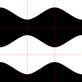
Figure 3. Left $(p,q)=(1,0)$, right $(p,q)=(3,0)$. In each case $\theta=1$. Note how the eigenfunction in the case $(3,0)$ is constructed by folding the (scaled) $(1,0)$ eigenfunction evenly.

Figure 4. Left $(p,q)=(3,0)$ with $\theta=\pi/4$, right $(p,q)=(3,0)$ with $\theta=3\pi/4$. Both these cases give the maximal cardinal of $8$ nodal domains.

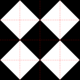
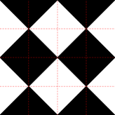
Figure 5. Left $(p,q)=(4,0)$ with $\theta=\pi/4$, right $(p,q)=(4,0)$ with $\theta=3\pi/4$. Note that $\theta=\pi/4$ gives $13$ nodal domains, which is the maximal cardinal, while $\theta=3\pi/4$ gives $12$ nodal domains, only.

Corollary 4.3.

The eigenvalues $\lambda_{10}=\lambda_{11}$, $\lambda_{16}=\lambda_{17}$, $\lambda_{34}=\lambda_{35}$, $\lambda_{44}=\lambda_{45}$, $\lambda_{57}=\lambda_{58}$, $\lambda_{72}=\lambda_{73}$, $\lambda_{105}=\lambda_{106}$, $\lambda_{122}=\lambda_{123}$, and $\lambda_{167}=\lambda_{168}$ are not Courant sharp.

4.2. The case $(p,p)$

Lemma 4.4.

If the eigenspace corresponding to $\lambda=2p^{2}$ is one-dimensional and $\Psi$ is an eigenfunction corresponding this eigenvalue, then $\mu(\Psi)=(p+1)^{2}$.

Proof.

The eigenspace is spanned by $\cos px\cos py$, which is a true product of a function depending on $x$ and one that depends on $y$. Each of them has $p$ zeros, and thus the number of nodal domains equals $(p+1)^{2}$. ∎

Corollary 4.5.

The eigenvalues $\lambda_{18}$, $\lambda_{32}$, $\lambda_{65}$, $\lambda_{86}$, $\lambda_{113}$, $\lambda_{140}$, and $\lambda_{206}$ are not Courant sharp.

5. Critical points, boundary points and the chessboard localization

The reasoning below depends on the fact that the number of nodal domains of a continuous curve of eigenfunctions $\Psi_{t}$ is constant unless there are interior stationary points appearing in the zero-set, i.e. $(x,y)\in\Omega$ such that

$$\Psi(x,y)=0,\quad\partial_{x}\Psi(x,y)=0,\quad\partial_{y}\Psi(x,y)=0\,,$$ (5.1)

or changes in the cardinal of the boundary points. We refer for this point to Lemma 4.4 in [13]. Hence the analysis of these situations is quite important.

5.1. Critical points

Lemma 5.1.

If $p+q$ is odd, and $0<\theta\leq\pi/4$, then $\Phi_{p,q}^{\theta}$ satisfies (5.1) at the point $(x,y)$ in $\Omega$ if and only if

$$p\tan px=q\tan qx\,,\quad\text{and}\quad p\tan py=q\tan qy\,.$$ (5.2)

If these two equations are fulfilled, we recover the critical value of $\theta$ via

$$\tan\theta=-\frac{\cos qx\cos py}{\cos px\cos qy}\,.$$ (5.3)

Proof.

The eigenfunctions have the form

$$\Phi_{p,q}^{\theta}(x,y)=\cos\theta\cos qx\cos py+\sin\theta\cos qy\cos px\,.$$

The zero critical points are determined by

$$\cos\theta\cos qx\cos py+\sin\theta\cos qy\cos px =0\,,$$

$$q\cos\theta\sin qx\cos py+\sin\theta p\cos qy\sin px =0\,,\quad\text{and}$$

$$p\cos\theta\cos qx\sin py+q\sin\theta\sin qy\cos px =0\,.$$

Since $0<\theta\leq\pi/4$, the critical points $(x,y)$ should satisfy (5.2). (Note that one can reduce by dilation to the case when $p$ and $q$ are mutually prime.)

Once a pair satisfying these two conditions is given, we recover the corresponding critical values of $\theta$ by (5.3). ∎

5.2. Boundary points

The intersection of the zero set of $\Phi^{\theta}_{p,q}$ with the boundary is determined by the equations

$$\Phi^{\theta}_{p,q}(0,y)=0 \iff\frac{\cos py}{\cos qy}=-\cot\theta,$$ (5.4)

$$\Phi^{\theta}_{p,q}(\pi,y)=0 \iff\frac{\cos py}{\cos qy}=\cot\theta,$$

$$\Phi^{\theta}_{p,q}(x,0)=0 \iff\frac{\cos px}{\cos qx}=-\tan\theta,$$

$$\Phi^{\theta}_{p,q}(x,\pi)=0 \iff\frac{\cos px}{\cos qx}=\tan\theta,$$

Outside the zeros of $x\mapsto\cos qx$, the function

$$f_{p,q}(x)=\frac{\cos px}{\cos qx}\,$$ (5.5)

has derivative

$$f_{p,q}^{\prime}(x)=\frac{-p\sin px\cos qx+q\cos px\sin qx}{\cos^{2}qx}\,.$$

Is it easy from the graph of $f_{p,q}$ to count for a given $\theta$ the number of points arriving at the boundary. Except at the corners (see Remark 5.3 below) this number is changing at the critical values of $f_{p,q}$ (see Remark 5.2), which are the solutions of

$$p\tan px=q\tan qx\,.$$ (5.6)

5.3. Guide for the case by case analysis

In the case by case analysis we will always have in mind the following remarks.

Remark 5.2.

The critical points at the boundary (except for the corners) are given by $(0,x_{i})$, $(x_{i},0)$, $(\pi,x_{i})$ and $(x_{i},\pi)$ where $x_{i}$ is some non zero solution of (5.6). The corresponding critical $\theta$ is obtained by equation (5.4).

Remark 5.3.

The values for which lines arrive to the corner correspond only to $\theta=\frac{\pi}{4}$ and $\theta=\frac{3\pi}{4}$.

Remark 5.4.

The solutions of $p\tan px=q\tan qx$ can also be obtained by looking at the local extrema of $f_{p,q}\,$.

Remark 5.5.

The analysis of the solutions of $p\tan px=q\tan qx$ can (by a change of variable) be reduced to the case when $p$ and $q$ are mutually prime.

From these remarks, we deduce that for a complete analysis of the nodal patterns corresponding to a pair $(p,q)$ such that the eigenvalue $p^{2}+q^{2}$ has multiplicity $2$, we should first analyze the graph of the function $f_{p,q}\,$. This will not only permit to count in function of $\theta$ the number of lines touching the boundary but will also permit to determine by the analysis of the local extrema to determine the critical value of $\theta$ for which we have critical points.

5.4. Chessboard argument and applications

This idea was proposed by A. Stern [18] and used intensively and more rigorously in [1, 2, 3]. We consider a pair $(p,q)$ with $(p,q)$ mutually prime and $p+q$ odd and would like to localize the zeros of $\Phi_{p,q}^{\theta}$ for say $\theta\in(0,\frac{\pi}{2})$. It is based on a very elementary observation. We simply observe that if $\cos px\cos py\cos qx\cos qy>0$, then $\Phi^{\theta}\neq 0$. This determines the “white” rectangles of a chessboard. These rectangles are obtained by drawing the vertical lines $\{x=k\frac{\pi}{2p}\}$ ($k$ odd) and $\{x=k^{\prime}\frac{\pi}{2q}\}$ ($k^{\prime}$ odd), and similarly the horizontal lines $\{y=k\frac{\pi}{2p}\}$ ($k$ odd) and $\{y=k^{\prime}\frac{\pi}{2q}\}$ ($k^{\prime}$ odd), and hence the zero set should be contained in the closed “black” rectangles corresponding to the closure of the set $\{\cos px\cos py\cos qx\cos qy<0\,\}$. Note that these rectangles have different size. It is also important to determine which points at the boundary of a given rectangle belongs to the zero set. They are obtained by the equations $(x,y)=(k\frac{\pi}{2p},k^{\prime}\frac{\pi}{2p})$ and for $(x,y)=(\ell\frac{\pi}{2q},\ell^{\prime}\frac{\pi}{2q})$ for $k$, $\ell$, $k^{\prime}$, $\ell^{\prime}$ odd. So the nodal set should contain all these points and only these points. We call these points admissible corners. This can also be seen as a consequence of the fact that $\cos px$ and $\cos qx$ have no common zero in $[0,\pi]$ when $p+q$ is odd. Hence we have proved.

Lemma 5.6.

If $p$ and $q$ are mutually prime and $p+q$ is odd, and $\theta\in(0,\frac{\pi}{2})$ then the only points of intersection of the zero set of $\Phi_{p,q}^{\theta}$ with the boundary of a black rectangle are the admissible corners.

Moreover, these points are regular points of the zero set.

Another point is that the zero set cannot contain any closed curve inside a black rectangle (we also mean curves touching the boundary). The ground state energy inside the curve delimited by the curve (say in the case without double points) should indeed be strictly above the ground state energy of the rectangle (Dirichlet for a rectangle in the interior, Dirichlet–Neumann when the rectangle has at least one size common to the square $[0,\pi]^{2}$). But the minimal energy for these rectangles is $2\max(p,q)^{2}$ (a contradiction with the value $p^{2}+q^{2}$).

Lemma 5.7.

If $p$ and $q$ are mutually prime and $p+q$ is odd and $\theta\in(0,\frac{\pi}{2})$ then the zero set of $\Phi_{p,q}^{\theta}$ cannot contain any closed curve contained in a ”black” rectangle.

Remark 5.8.

As a consequence of these two lemmas let us observe that at an admissible corner only one curve belonging to the zero set can enter in a black rectangle and that it should either go out by an admissible corner, either touch the boundary or meet another curve of the zero set at a critical point.

6. Special cases

Most of the cases appearing in the table are treated via the general considerations of Sections 2 and 3. In this section, we consider a first list of special cases where a more careful analysis is needed, which involves the analysis of boundary points or of critical points.

6.1. The case $\lambda_{7}=\lambda_{8}=5$ ($(p,q)=(2,1)$)

The eigenspace is two-dimensional,

$$\Phi_{2,1}^{\theta}(x,y)=\cos\theta\cos 2x\cos y+\sin\theta\cos x\cos 2y\,,\quad 0\leq\theta<\pi\,.$$ (6.1)

We know from Lemma 3.1 that this case is not Courant sharp, but that it has a maximum number of nodal domains being $6$.

Lemma 6.1.

$\mu(\Phi_{2,1}^{0})=6$. If $0<\theta\leq\pi/4$ then $\mu(\Phi_{2,1}^{\theta})=4\,$.

Proof.

Observing that $\tan 2x=2\tan x/(1-\tan^{2}x)$ it is immediate that

$$2\tan 2x=\tan x$$

has no zero in the open interval $(0,\pi)$. Hence by Lemma 5.1, there are no critical points for $\Phi_{1,2}$ in $\Omega$. Having in mind (5.4), the analysis of the graph

$$f_{2,1}(x)=\cos 2x/\cos x=(2\cos^{2}x-1)/\cos x$$

(see Figure 6) leads immediately (see Figure 7 for $\theta=\frac{\pi}{8}$) to the existence of $4$ nodal domains in this case (two boundary points for $y=0$ and $y=\pi$ and one boundary point for $x=0$ and $x=\pi$).

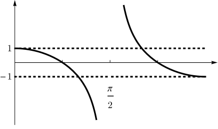
Figure 6. The graph of $f_{2,1}(x)=\frac{\cos(2x)}{\cos(x)}$ in the interval $0<x<\pi$.

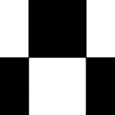
Figure 7. Nodal domains for $\Phi_{2,1}^{\theta}$ when $\theta=0$, $\theta=\pi/8$, and $\theta=\pi/4$.

It remains to consider two cases, $\theta=0$ and $\theta=\frac{\pi}{4}$. For $\theta=0$ we are in the product case and have $6$ nodal domains. For $\theta=\pi/4$ we let $u=\cos x$ and $v=\cos y$, both living in $[-1,1]$. Then

$$\Phi_{2,1}^{\pi/4}(x,y)=0 \iff(2u^{2}-1)v+u(2v^{2}-1)=0$$

$$\iff(u+v)(2uv-1)=0\,.$$

Thus, we get the straight line $u=-v$ and the hyperbola $4uv=1$. We note that they do not intersect. Thus, there are $4$ nodal domains in this case. ∎

6.2. The case $\lambda_{21}=\lambda_{22}=20$ ($(p,q)=(4,2)$)

Lemma 6.2.

Assume that $(\lambda_{21},\Psi_{21})$ is an eigenpair of $L$. Then $\mu(\Psi_{21})\leq 15$. In particular we are not in the Courant sharp situation.

Proof.

If $\theta\not\in\{0,\pi/2\}$, then Lemmas 3.8 and 6.1 give that the number of nodal domains is less than or equal to $4\cdot 4-3=13$. For $\theta\in\{0,\pi/2\}$ we are in the product case, and have $15$ nodal domains. ∎

6.3. The case $\lambda_{70}=\lambda_{71}=80$ ($(p,q)=(8,4)$)

Lemma 6.3.

Assume that $(\lambda_{70},\Psi_{70})$ is an eigenpair of $L$. Then $\mu(\Psi_{70})\leq 57\,$. In particular we are not in the Courant sharp situation.

Proof.

If $\theta\not\in\{0,\pi/2\}$, then Lemmas 3.8 and 6.2 imply that the number of nodal domains is less than or equal to $4\cdot 15-3=57\,$. For $\theta\in\{0,\pi/2\}$ we are in the product case, and have $45$ nodal domains. ∎

6.4. The case $\lambda_{42}=\lambda_{43}=45$ ($(p,q)=(6,3)$)

Lemma 6.4.

Assume that $(\lambda_{42},\Psi_{42})$ is an eigenpair of $L$. Then $\mu(\Psi_{42})\leq 36\,$. In particular, the eigenpair $(\lambda_{42},\Psi_{42})$ is not Courant sharp.

Proof.

Fix $\theta\in[0,\pi)$. It holds that $\Phi_{6,3}^{\theta}(x,y)=\Phi_{2,1}^{\theta}(3x,3y)$ in the square $\{(x,y)~{}|~{}0<x<\pi/3,\ 0<y<\pi/3\}$. Moreover, the values of $\Phi_{6,3}^{\theta}$ in the rest of $\Omega$ are recovered by “folding evenly”. Thus, the number of nodal domains are less then or equal to (in fact, this could be made sharper) nine times the number of nodal domains of $\Phi_{2,1}^{\theta}\,$.

From Lemma 6.1 it follows that if $\theta\not\in\{0,\pi/2\}$ then

$$\mu(\Phi_{6,3}^{\theta})\leq 9\times 4=36\,.$$

If $\theta\in\{0,\pi/2\}$ then we are in the product case and have $28$ nodal domains. ∎

6.5. The case $\lambda_{14}=\lambda_{15}=13$ ($(p,q)=(3,2)$)

Here the situation is similar to $(p,q)=(2,1)$, but with one additional nodal domain touching each part of the boundary. The general eigenfunction is

$$\Phi_{3,2}^{\theta}(x,y)=\cos\theta\cos 3x\cos 2y+\sin\theta\cos 2x\cos 3y\,,\quad 0\leq\theta<\pi\,.$$ (6.2)

Lemma 6.5.

If $\theta=0$ then $\mu(\Phi_{3,2}^{0})=12$. If $0<\theta\leq\pi/4\,$, $\mu(\Phi_{3,2}^{\theta})=6\,$. In particular, if $(\lambda_{14},\Psi_{14})$ is an eigenpair of $L$, it is not Courant sharp.

Proof.

By Lemma 3.10 it is sufficient to consider $0\leq\theta\leq\pi/4\,$.

If $\theta=0$ we are in the product case and there are exactly $12$ nodal domains.

Assume that $0<\theta\leq\pi/4$. Let us start to count the nodal lines that touch the boundary. For this, we use (5.4) with $(p,q)=(3,2)$. The function $f_{3,2}(x)=\frac{\cos 3x}{\cos 2x}$, $x\in[0,\pi]\setminus\{\pi/4,3\pi/4\}$ has derivative

$$f_{3,2}^{\prime}(x)=-\frac{(3+\cos 2x+\cos 4x)\sin x}{\cos^{2}2x}.$$

Figure 8. The graph of $f_{3,2}(x)=\frac{\cos(3x)}{\cos(2x)}$ in the interval $0<x<\pi$.

In particular, $f_{3,2}^{\prime}$ is negative where it is defined. We find immediately that $f_{3,2}$ attains all values in $[-1,1]$ three times and all values in $\mathbb{R}\setminus\{[-1,1]\}$ twice.

Using Lemma 5.1 and Remark 5.4 and the fact that $f_{3,2}$ has no critical points in its domain of definition, we get that we have no interior critical points of $\Phi_{3,2}^{\theta}$. We conclude (see for example Figure 9 for $\theta=\frac{\pi}{8}$) that if $0<\theta<\pi/4$ then we have exactly three nodal lines touching each part of the boundary of $\Omega$ where $y=0$ and $y=\pi$, and exactly two nodal lines on each of the parts of the boundary of $\Omega$ where $x=0$ and $x=\pi$.

Thus, we only have to consider the case $\theta=\pi/4$. If $\theta=\pi/4$ then we have one nodal line $y=\pi-x$ and two additional nodal lines touching each part of the boundary.

Next, we eliminate the case of loops in the zero set by using Lemma 5.7. In this simple case, we can do a more algebraic computation. We make the substitution $u=\cos x$ and $v=\cos y$ and find that $\Phi_{3,2}^{\pi/4}(x,y)=0$ if and only if

$$(u+v)\bigl{(}8u^{2}v^{2}-4u^{2}-4v^{2}-2uv+3\bigr{)}=0\,.$$

One solution is $u=-v$. Let $F(u,v)=8u^{2}v^{2}-4u^{2}-4v^{2}-2uv+3\,$. Then $F^{\prime}_{v}=16u^{2}v-8v-2u$ and hence

$$F^{\prime}_{v}=0\iff v=\frac{u}{4(2u^{2}-1)}\,,\quad u\neq\pm 1/\sqrt{2}\,.$$

It is easily seen that $F^{\prime}_{v}(\pm 1/\sqrt{2},v)=\mp\sqrt{2}\neq 0\,$. Next,

$$F\Bigl{(}u,\frac{u}{4(2u^{2}-1)}\Bigr{)}=\frac{32u^{4}-39u^{2}+12}{4(1-2u^{2})}\,,$$

and since $1521=39^{2}<4\cdot 32\cdot 12=1536$ we find that $F$ and $F^{\prime}_{v}$ have no common zeros. Thus, the nodal lines are never vertical. By symmetry in $u$ and $v$ it follows that they are never horizontal either.

All in all, this means that for $\theta=\pi/4$ (and thus for $0<\theta\leq\pi/4$) we have five non-intersecting nodal lines, and so six nodal domains. ∎

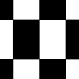
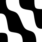
Figure 9. Nodal domains for $\Phi_{3,2}^{\theta}$ when $\theta=0$, $\theta=\pi/8$, and $\theta=\pi/4\,$.

6.6. The case $\lambda_{49}=\lambda_{50}=52$ ($(p,q)=(6,4)$)

Lemma 6.6.

If $\theta\in\{0,\pi/2\}$ then $\mu(\Phi_{6,4}^{\theta})=35\,$. For all other values of $\theta\,$, $\mu(\Phi_{6,4}^{\theta})\leq 21\,$. In particular, if $(\lambda_{49},\Psi_{49})$ is an eigenpair of $L\,$, then it is not Courant sharp.

Proof.

If $\theta\in\{0,\pi/2\}$ then we are in the product case, and have $(6+1)\times(4+1)=35$ nodal domains.

If $\theta\not\in\{0,\pi/2\}$ then, combining Lemmas 3.8 and 6.5, we find that the number of nodal domains are at most $4\cdot 6-3=21$. ∎

7. Four remaining cases

It remains to analyze the four cases $(4,1)$, $(8,3)$, $(9,4)$, and $(10,4)$. We will start by a detailed analysis of the case $(4,1)$. For the last three cases we will use a chessboard localization to improve the estimate $|\Omega^{\text{inn}}|\leq|\Omega|$ used in Section 2 (see Lemma 2.2).

7.1. The case $\lambda_{18}=\lambda_{19}=17$ ($(p,q)=(4,1)$)

Lemma 7.1.

For any $\theta$, $\mu(\Phi_{4,1}^{\theta})\leq 10$. The possible values of $\mu(\Phi_{4,1}^{\theta})$ are $6$, $8$ and $10$. In particular, if $(\lambda_{18},\Psi_{18})$ is an eigenpair of $L$, then it is not Courant sharp.

Proof.

The case $\theta=0$ being very simple to analyze (product situation, $10$ nodal domains, hence not Courant sharp). By Lemma 3.10, it is sufficient to do the analysis for $\theta\in(0,\frac{\pi}{4}]$.

Step 1: analysis of the graph of $f_{4,1}$

As explained in Section 5, everything can be read on the graph of $f_{4,1}$.

Figure 10. The graph of $f_{4,1}(x)=\frac{\cos(4x)}{\cos(x)}$ in the interval $0<x<\pi$.

From the graph, we find that $f_{4,1}$ attains all values in $]-1,1[$ four times, and all values in $\mathbb{R}\setminus\{[-1,1]\}$ three, two or one times. This transition has to be analyzed further. Looking at the local extrema of $f_{4,1}$, there are two points $x_{1}$ and $x_{2}$ which are solutions for (5.6).

$$x_{1}=\arctan\sqrt{2\sqrt{10}-5}\approx 0.86,\quad\text{and}\quad x_{2}=\pi-\arctan\sqrt{2\sqrt{10}-5}\approx 2.29.$$

We can now follow the scheme of analysis presented in Section 5.

Step 2 : Interior critical points.

Using the symmetry of $x_{1}$ and $x_{2}$ with respect to $\frac{\pi}{2}$, we get that, for $\theta\in(0,\frac{\pi}{4}]$, the only stationary points of $\Phi_{4,1}^{\theta}$ are $(x_{1},x_{2})$ and $(x_{2},x_{1})$ and appear when $\theta=\pi/4$.

So we need a special analysis for $\theta=\frac{\pi}{4}$. From Figure 11 we see that the number of nodal domains is $10$. We immediately see that the anti-diagonal belongs to the zero set.

Step 3: Analysis of the boundary points

Here we have to use (5.4) for $(p,q)=(4,1)$ and our preliminary analysis of the graph of $f_{4,1}$. We conclude that if $0<\theta<\pi/4$ then we have exactly four nodal lines touching each part of the boundary of $\Omega$ where $y=0$ and $y=\pi$, BUT the number of nodal lines on each of the parts of the boundary of $\Omega$ where $x=0$ and $x=\pi$ can be $1$, $2$ or $3$. There is another critical value $\theta_{1}\in(0,\frac{\pi}{4})$ corresponding to a local maximum of $f_{4,1}$:

$$\cot\theta_{1}=f_{4,1}(x_{2})\,.$$

One touching occurs at $(0,x_{1})$ and simultaneously at $(\pi,x_{2})$. It remains to count the number of nodal domains in this situation and to count the number of nodal domains for one value of $\theta\in(\theta_{1},\frac{\pi}{4})$.

In each of these intervals two strategies are possible:

• analyze perturbatively the situation for $\theta$ close to one of the ends of the interval;

• choose one specific value of $\theta$ in the interval.

In our case, we have finally three critical values of $\theta$ ($0$, $\theta_{1}$ and $\frac{\pi}{4}$) and two values to choose in $(0,\theta_{1})$ and $(\theta_{1},\frac{\pi}{4})$. Because $\theta_{1}\in(\frac{\pi}{8},\frac{\pi}{4})$, the picture for $\theta=\pi/8$ in Figure 11 is the answer in the interval $(0,\theta_{1})$. Hence, we see six nodal domains when $\theta\in(0,\theta_{1})$.

It remains to analyze the situation for $\theta=\theta_{1}$ and to analyze another case in $(\theta_{1},\frac{\pi}{4})$. We observe $8$ nodal domains for $\theta\in[\theta_{1},\frac{\pi}{4})$ and come back to $10$ for $\theta=\frac{\pi}{4}$. But this is the $18$-th eigenvalue.

                       

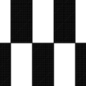
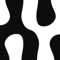
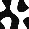
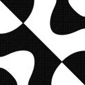
Figure 11. The graphs show nodal domains in the case $(p,q)=(4,1)$. From left to right, $\theta=\pi/8$, $\theta=\theta_{1}\approx 0.60$, $\theta=\pi/4-0.1$ and $\theta=\pi/4$.

Step 4: chessboard localization

We refer to Section 5 and particularly to the Lemmas 5.6 and 5.7. We now consider $\theta$ in the interval $(0,\theta_{1})$. We know that there are no critical points inside. Hence one line entering in a rectangle by one of the admissible corner belonging to the nodal set should exit the black rectangle by another corner or by the boundary. Conversely, a line starting from the boundary should leave the black rectangle through a corner in the zero set. Note that contrary to the case considered in [1] it is not true that all the corners belong to the zero set.

We now look at the points on the boundary. For $x=0$, we have shown that there is only one point $(0,y_{1})$. Moreover $y\in(\frac{\pi}{2},\frac{5\pi}{8})$. Similar considerations can be done to localize the four points on $y=0$ and on $y=\pi$. These localization are independent of $\theta\in(0,\theta_{1})$. Finally, we notice that $x=\pi/2$ meets the nodal set at a unique point $(\pi/2,\pi/2)$ and the same for $y=\frac{\pi}{2}$. It is then easy to verify that one can reconstruct uniquely the nodal picture using these rules.

For $\theta=\theta_{1}$ and $\theta\in(\theta_{1},\frac{\pi}{4})$, similar arguments lead to a unique topological type. For $\theta=\frac{\pi}{4}$, one should first analyze the neighborhood of the anti-diagonal where critical points are present.

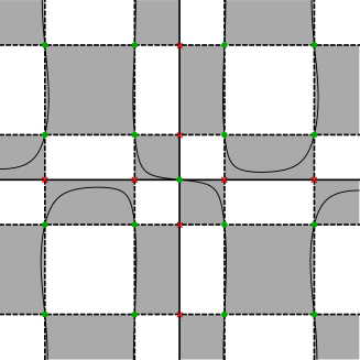
Figure 12. $(p,q)=(4,1)$, $\theta=0.1\,$.

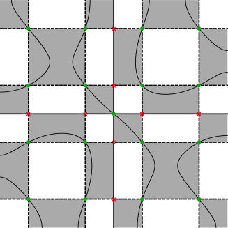
Figure 13. $(p,q)=(4,1)$, $\theta=\pi/4-0.1$.

∎

7.2. The case $\lambda_{66}=\lambda_{67}=73$ ($(p,q)=(8,3)$)

Lemma 7.2.

Let $(\lambda_{66},\Psi_{66})$ be an eigenpair of $L$. Then $\mu(\Psi_{66})\leq 56$. In particular, $(\lambda_{66},\Psi_{66})$ is not Courant sharp.

Proof.

By Lemma 3.10 it is sufficient to estimate the nodal domains of $\Phi_{8,3}^{\theta}$ for $0\leq\theta\leq\pi/4$. First, we note that for $\theta=0$ we are in the product situation and have $36$ nodal domains.

Next, we use the chessboard argument. For all $0<\theta\leq\pi/4$ it holds that the function $\cos 8x\cos 3y\cos 3x\cos 8y>0$ in the white rectangles. Thus no nodal lines can cross white rectangles. Moreover, since both $\cos\theta\neq 0$ and $\sin\theta\neq 0$, we find that the nodal lines must pass corners where both $\cos 8x\cos 3y$ and $\cos 3x\cos 8y$ are zero, and that they cannot pass corners where only one of them are zero (marked with a red cross). In Figure 14, we paint white rectangles blue in the following way: First we let each white rectangle touching the boundary become blue. Then we paint each white rectangle having a forbidden corner (marked with a red cross) in common with a blue rectangle. This latter procedure is repeated until it does not apply anymore. The so recolored blue rectangles are then necessarily all subsets of $\Omega^{\text{out}}$ of nodal domains touching the boundary. Note that this construction is independent of $\theta$. Thus,

$$|\Omega^{\text{out}}|\geq\pi^{2}\Bigl{[}\tfrac{1}{2}-8\times\bigl{(}\tfrac{1}{8}\bigr{)}^{2}\Bigr{]}=\tfrac{3}{8}\pi^{2},$$

and hence

$$|\Omega^{\text{inn}}|\leq\tfrac{5}{8}\pi^{2}.$$

Then Lemma 2.2 gives,

$$\mu(\Psi_{66})\leq\frac{|\Omega^{\text{inn}}|}{\pi j_{0,1}^{2}}\lambda_{66}+4\lfloor\sqrt{\lambda_{66}}\rfloor\leq\frac{365\,\pi}{8\,j_{0,1}^{2}}+32\approx 56.8.\qed$$

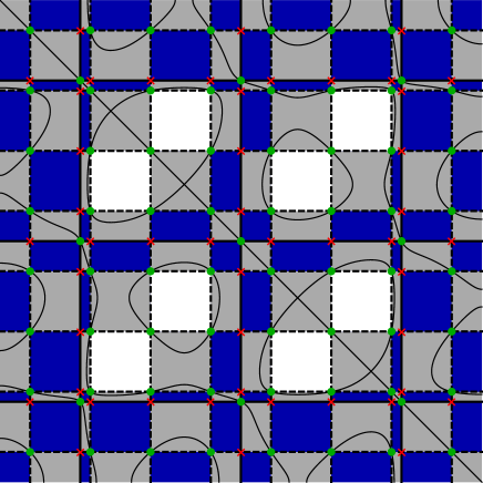
Figure 14. The case $(p,q)=(8,3)$, $\theta=\frac{\pi}{4}$.

7.3. The case $\lambda_{84}=\lambda_{85}=97$ ($(p,q)=(9,4)$)

Lemma 7.3.

Let $(\lambda_{84},\Psi_{84})$ be an eigenpair of $L$. Then $\mu(\Psi_{84})\leq 71$. In particular, $(\lambda_{84},\Psi_{84})$ is not Courant sharp.

Proof.

This proof goes line by line as the proof of Lemma 7.2, with a change of numbers only. For $\theta=0$ we are in the product situation, with $50$ nodal domains. Here, the blue area of Figure 15 equals $\tfrac{211}{648}\,\pi^{2}$, and so we know that $\Omega^{\text{out}}$ has this lower bound. This means that

$$|\Omega^{\text{inn}}|\leq\tfrac{437}{648}\pi^{2}\,.$$

We get from Lemma 2.2

$$\mu(\Psi_{84})\leq\frac{|\Omega^{\text{inn}}|}{\pi\,j_{0,1}^{2}}\lambda_{84}+4\lfloor\sqrt{\lambda_{84}}\rfloor\leq\frac{42389\,\pi}{648\,j_{0,1}^{2}}+36\approx 71.5.\qed$$

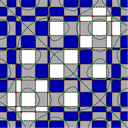
Figure 15. The case $(p,q)=(9,4)$, $\theta=\frac{\pi}{4}$.

7.4. The case $\lambda_{101}=\lambda_{102}=116$ ($(p,q)=(10,4)$)

Lemma 7.4.

Let $(\lambda_{101},\Psi_{101})$ be an eigenpair of $L$. Then $\mu(\Psi_{101})\leq 89$. In particular, $(\lambda_{101},\Psi_{101})$ is not Courant sharp.

Proof.

We first note that we are in the product situation if $\theta=0$ or $\theta=\pi/2$, with $55$ nodal domains. Since $\cos(10x)$ and $\cos(4x)$ have no common zeros, we can again apply the chessboard argument for $0<\theta<\pi/2$. For $\pi/2<\theta<\pi$ the argument is exactly the same, but with the roles of white and black rectangles interchanged.

Thus, as in the previous proofs, we count the area of the blue region, see Figure 16. We find that it equals $\tfrac{21}{100}\pi^{2}$.

Hence $|\Omega^{\text{inn}}|\leq\tfrac{79}{100}\pi^{2}$, and by Lemma 2.2

$$\mu(\Psi_{101})\leq\frac{|\Omega^{\text{inn}}|}{\pi j_{0,1}^{2}}\lambda_{101}+4\lfloor\sqrt{\lambda_{101}}\rfloor\leq\frac{2291\pi}{25j_{0,1}^{2}}+40\approx 89.8.\qed$$

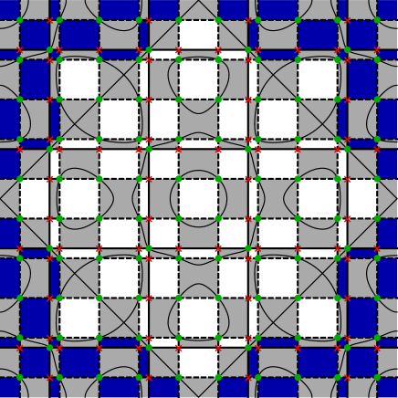
Figure 16. The case $(p,q)=(10,4)$, $\theta=\frac{\pi}{4}$.

With the proof of this last statement and the analysis presented in the table we have achieved the proof of Theorem 1.1. In the next section we will by curiosity analyze the spectral pattern of some of the families.

8. Optimal calculations

Although not used in the proof of the main results in this paper, we present in the spirit of the analysis of the case $(4,1)$ a complete analysis of the nodal pattern in the cases $(5,2)$ and $(8,3)$.

8.1. The case $\lambda_{29}=\lambda_{30}=29$ ($(p,q)=(5,2)$)

We already know that we are not Courant sharp by Lemma 3.1. It does not cost too much (an application could be for the analysis of the case $(10,4)$ but we only need a weaker upper bound) to establish the

Proposition 8.1.

For any $\theta$, we have the optimal bound $\mu(\Phi_{5,2}^{\theta})\leq 18\,$.

The analysis of the equation $5\tan 5x=2\tan 2x$ leads to the existence of two positive solutions $(x_{1},x_{2})$ of this equation with

$$0<\frac{\pi}{4}<x_{1}<\frac{\pi}{2}<x_{2}=\pi-x_{1}\,.$$

These values appear also as the critical values of $f_{5,2}(x)$ as can be seen in Figure 17.

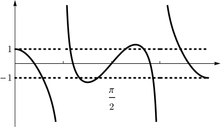
Figure 17. The graph of $f_{5,2}(x)=\frac{\cos(5x)}{\cos(2x)}$ in the interval $0<x<\pi$.

It is sufficient to analyze the situation for $\theta\in(0,\frac{\pi}{4}]$. The discussion is rather close to the case $(4,1)$.

For $\theta=0$, we start from $3\times 6$ nodal domains. We have indeed $10$ critical points and $14$ boundary points (avoiding the corners). In the interval $(0,\frac{\pi}{4})$, there are no critical point inside the square. But there are transition at the boundary for $\theta_{1}\in(0,\frac{\pi}{4})$ such that $\tan\theta_{1}=1/f_{5,2}(x_{2})$. Hence the number of nodal domains is fixed in $(0,\theta_{1})$ and because when starting from $0$, we have only opening at the former crosses, the number of nodal domains can only decrease. More precisely, the number of nodal domain is eight.

                       

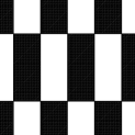
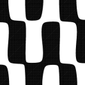
Figure 18. The graphs show nodal domains in the case $(p,q)=(5,2)$. From left to right, $\theta=0$, $\theta=0.1$, $\theta=\theta_{1}\approx 0.65$, $\theta=\pi/4-0.1$ and $\theta=\pi/4$.

This results from the numerics or the perturbative analysis starting from $\theta=0$. An analysis for $\theta=\theta_{1}$ should be done. Then again the number of nodal domains is fixed in $(\theta_{1},\frac{\pi}{4})$ and equal to $10$.

At $\theta=\frac{\pi}{4}$, the nodal set contains the anti-diagonal $y=\pi-x$. The number of boundary points outside the corners become $4$ on each side. We have two critical points $(x_{1},x_{2})$ and $(x_{2},x_{1})$ on the anti-diagonal. Numerics permits us to determine the number of nodal domains, which increases by $2$ and is equal to $10$ for $\theta=\frac{\pi}{4}$.

We keep in mind the results established in Section 5 on the chessboard localization. We now consider $\theta$ in the interval $(0,\theta_{1})$. We know that there are no critical points inside. Hence one line entering in a rectangle by one of the corners belonging to the nodal set should exit the black rectangle by another corner or by the boundary. Conversely, a line starting from the boundary should leave the black rectangle through a corner in the zero set. Note that contrary to the case considered in [1] it is not true that all the corners belong to the zero set.

We now look at the points on the boundary. For $x=0$, we have shown that there are exactly two points $(0,\eta_{1})$ and $(0,\eta_{2})$. Moreover $\eta_{1}\in(\frac{\pi}{10},\frac{\pi}{4})$ and $\eta_{2}\in(\frac{7\pi}{10},\frac{3\pi}{4})$. Similar considerations can be done to localize the five points on $y=0$, $\xi_{1},\xi_{2},\xi_{3},\xi_{4},\xi_{5}$, and on $y=\pi$, $\xi^{\prime}_{1},\dots,\xi^{\prime}_{5}$, and two points on $x=\pi$, $\eta^{\prime}_{1},\eta^{\prime}_{2}$. These localizations are independent of $\theta\in(0,\theta_{1})$.

Let us see if one can reconstruct uniquely the (topology of the) nodal picture using these rules.
The nodal line starting from the boundary at $(0,\eta_{1})$ has no choice (that is the ordered sequence of admissible corners which are visited is uniquely determined) and should arrive to $(\xi_{1},0)$. The line starting of $(0,\eta_{2})$ has no choice and should arrive to $(\xi_{2},0)$. The line starting from $(\xi^{\prime}_{2},\pi)$ should come back to $(x^{\prime}_{3},\pi)$. The line starting from $(x^{\prime}_{4},\pi)$ is obliged to go to $(\pi,\eta^{\prime}_{1})$ and the line starting from $(\xi^{\prime}_{5},\pi)$ has to go to $(\pi,\eta^{\prime}_{2})$. All these lines are unique. It remains one line which has to go from $(\xi^{\prime}_{1},\pi)$ to $(\xi_{5},0)$ with the obligation to visit all the elements of the two lattices which have not been visited before. A small analysis shows that it remains two possible paths around the center (see Figure 19).

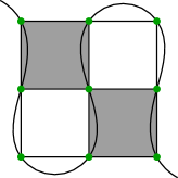
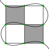
Figure 19. The two alternatives in the central square (consisting of four smaller squares). The left alternative is the right one in the next figure.

Hence we need an additional argument to fix the sequence of visited admissible corners. For example it is enough to show that on the line $x=\frac{2\pi}{5}$ there are no zero $(\frac{2\pi}{5},y)$ with $y\in(\frac{\pi}{2},\frac{7\pi}{10})$. This is at least clear for $\theta$ small and because no critical point can appear before $\theta=\frac{\pi}{4}$. We are done with this case.

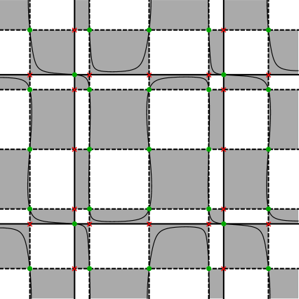
Figure 20. $(p,q)=(5,2)$, $\theta=0.1$.

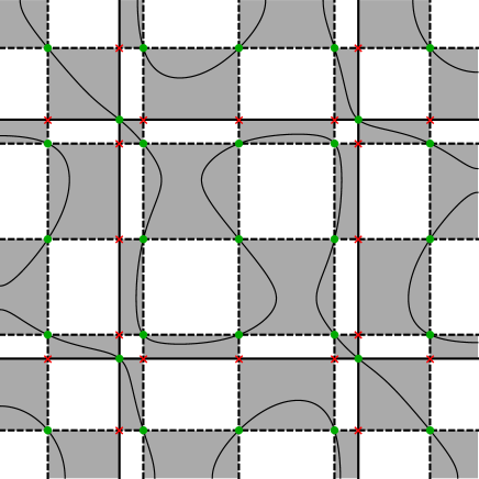
Figure 21. $(p,q)=(5,2)$, $\theta=\pi/4-0.1$.

For $\theta\in(\theta_{1},\frac{\pi}{4})$, similar arguments lead to a unique topological type. We have now four points $(0,\eta_{j})$ ($j=1,\dots,4$) and four points $(\pi,\eta^{\prime}_{j})$ ($j=1,\dots,4$) at the vertical boundaries but except a change in the black rectangle containing $(0,\eta_{2})$ and $(0,\eta_{3})$ and the black rectangle containing $(\pi,\eta^{\prime}_{2})$ and $(\pi,\eta^{\prime}_{3})$, nothing changes outside. At a first sight, there are still two possibilities but the transition to the second possibility can only occur through a critical point. This is impossible before $\theta=\frac{\pi}{4}$.

Remark 8.2.

As a corollary, we recover that the eigenvalue $\lambda_{101}$ is not Courant sharp. This is an immediate consequence of Lemma 3.8 and Lemma 8.1. This gives:

$$\mu(\Phi_{10,4})\leq 69\,.$$

This can be improved by using the detailed case by case analysis of $\Phi^{\theta}_{5,2}$. We will then get the optimal upper-bound:

$$\mu(\Phi_{10,4})\leq 55\,,$$

to compare with Lemma 7.4.

8.2. The case $\lambda_{66}=\lambda_{67}=73$ ($(p,q)=(8,3)$)

Proposition 8.3.

For any $\theta$, we have the optimal bound $\mu(\Phi_{8,3}^{\theta})\leq 36\,$.

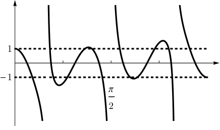
Figure 22. The graph of $f_{8,3}(x)=\frac{\cos(8x)}{\cos(3x)}$ in the interval $0<x<\pi$.

The analysis of the Figure 22 shows the existence of six critical points:

$$x_{0}=0<\frac{\pi}{6}<x_{1}<\frac{5\pi}{16}<x_{2}<\frac{\pi}{2}<x_{3}<x_{4}<\frac{5\pi}{6}<\pi=x_{5}\,,$$

with

$$x_{4}=\pi-x_{1}\,,\quad x_{3}=\pi-x_{2}\,.$$

We associate with these critical values the two positive numbers:

$$z_{1}=f_{8,3}(x_{2})\approx 1.10\,,\quad z_{2}=-f_{8,3}(x_{1})\approx 1.56\,,$$

and observe that

$$1<z_{1}<z_{2}\,.$$

Associated with $(z_{1},z_{2})$ we introduce the two critical angles in $(0,\frac{\pi}{4})$:

$$\tan\theta_{1}=1/z_{2}\,,\,\tan\theta_{2}=1/z_{1}\,.$$

For these two values some transition should appear at the boundary.

We now look at the interior critical points corresponding to pairs $(x_{i},x_{j})$ ($i=1,\dots,4)$ and $j=(1,\dots,4)$. The corresponding critical $\theta_{ij}$ are determined by

$$\tan\theta_{ij}=-f_{8,3}(x_{j})/f_{8,3}(x_{i})$$

with $\theta_{ij}\in(0,\pi)$.

Using the symmetries, it is enough to look at the ones which belong to $(0,\frac{\pi}{4}]$. We recover $\frac{\pi}{4}$ with any pair $(x_{i},\pi-x_{i})$ but we have also to consider $\theta_{13}$ which is determined by $z_{1}/z_{2}$. We observe (numerically) that

$$\frac{1}{z_{2}}<\frac{z_{1}}{z_{2}}<\frac{1}{z_{1}}\,.$$

Hence we have at the end to look at the values $0$, $\theta_{1}$, $\theta_{13}$, $\theta_{2}$ and $\frac{\pi}{4}$ and to four values of $\theta$ corresponding to each of the intervals $(0,\theta_{1})$, $(\theta_{1},\theta_{13})$, $(\theta_{13},\theta_{2})$ and $(\theta_{2},\frac{\pi}{4})$.

         

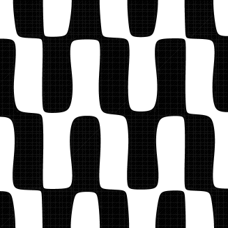
Figure 23. Nodal domains for $(p,q)=(8,3)$ and $\theta=0.1$ (12 nodal domains).

         

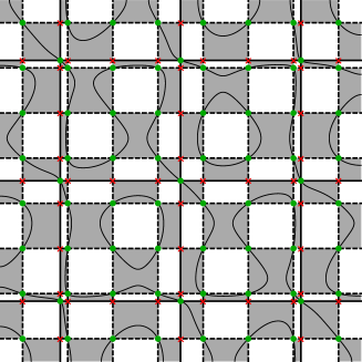
Figure 24. Nodal domains for $(p,q)=(8,3)$ and $\theta=\pi/4-0.1$ (16 nodal domains).

         

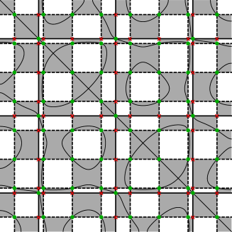
Figure 25. Nodal domains for $(p,q)=(8,3)$ and $\theta=\pi/4$ (22 nodal domains).

We keep in mind the results obtained in Section 5 concerning the chessboard localization and its consequences.
We now consider $\theta$ in the interval $(0,\theta_{1})$. We know that there are no critical points inside. Hence one line entering in a rectangle by one of the corner belonging to the nodal set should exit the black rectangle by another corner or by the boundary. Conversely, a line starting from the boundary should leave the black rectangle through a corner in the zero set.

We now look at the points on the boundary. For $x=0$, we have shown that there are exactly three points $(0,\eta_{1})$, $(0,\eta_{2})$, and $(0,\eta_{3})$. Moreover $\eta_{1}\in(\frac{\pi}{6},\frac{3\pi}{16})$, $\eta_{2}\in(\frac{\pi}{2},\frac{9\pi}{16})$, and $\eta_{3}\in(\frac{5\pi}{6},\frac{15\pi}{16})$. Similar considerations can be done to localize the nine points on $y=0$, $\xi_{1},\dots,\xi_{8}$, and on $y=\pi$, $\xi^{\prime}_{1},\dots,\xi^{\prime}_{8}$, and three points on $x=\pi$, $\eta^{\prime}_{1},\eta^{\prime}_{2},\eta^{\prime}_{3}$. These localizations are independent of $\theta\in(0,\theta_{1})$.

Let us see if one can reconstruct uniquely the nodal picture using these rules. The nodal line starting from $(0,\eta_{1})$ has no other choice than going through one admissible corner to the point $(\xi_{1},0)$. The nodal line starting from $(0,\eta_{2})$ has no other choice than going to $(\xi_{2},0)$ after passing through five admissible corners. The curve starting from $(\xi_{3},0)$ has no other choice than coming back to the same boundary at $(\xi_{4},0)$ after passing through two admissible corners. Similarly, the line starting from $(\xi_{6},0)$ has no other choice than coming back to the same boundary at $(\xi_{7},0)$ after passing through two admissible corners. For the nodal line starting from $(0,\eta_{3})$, the first five admissible corners to visit are uniquely determined by the given rules. Then the line enters in a rectangle with four admissible corners. There are two choices for leaving this rectangle. The determination of the right admissible corner can be done by using perturbation theory or a barrier argument. This leads to go down to the left down corner. After visiting this one the two next admissible corners are uniquely determined. The nodal line enters in a rectangle with four admissible corners. Again, we have to use a perturbation argument to decide that we have to leave at the admissible left up corner. Then everything is uniquely determined till the nodal line touches the boundary at $(\xi_{5},0)$. We now use the symmetry with respect to the diagonal to draw three new nodal lines.

The last line joining $(\xi^{\prime}_{1},\pi)$ to $(\xi_{8},0)$ is then uniquely determined. In this way we get twelve nodal domains.

The case $\theta=\theta_{1}$ corresponds to a change at the boundary. Instead of three lines touching at the boundary at $x=0$ and $x=\pi$, two new lines touch the boundary at the same point at $x=0$ between the former $(0,\eta_{1})$ and $(0,\eta_{2})$ (resp at $x=\pi$ between $(\pi,\eta^{\prime}_{2})$ and $(\pi,\eta^{\prime}_{3})$). The number of nodal domains becomes equal to $14$.

For $\theta\in(\theta_{1},\theta_{13})$, nothing has changed except that we have now exactly five points at $x=0$ and five points at $x=\pi$. The number of nodal domains is constant and equal to $14$.

For $\theta=\theta_{13}$, two critical points appear inside the square leading to the creation of two new nodal domains. We have now sixteen nodal domains. Nothing has changed at the boundary.

For $\theta\in(\theta_{13},\theta_{2})$, the two critical points disappear. Nothing changes at the boundary and we keep $16$ nodal domains.

For $\theta=\theta_{2}$, two new lines touch the boundary at the same point at $x=0$ and similarly at $x=\pi$. This creates two new nodal domains. We now get $18$ nodal domains.

For $\theta\in(\theta_{13},\frac{\pi}{4})$, we have now seven touching points at $x=0$ and seven at $x=\pi$. The number of nodal domains remains equal to $18$.

Finally, for $\theta=\frac{\pi}{4}$, four critical points appear on the anti-diagonal. Four nodal domains are created. We have now $22$ nodal domains.

This ends the (sketch of) the proof of Proposition 8.3.

           
           
           

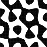
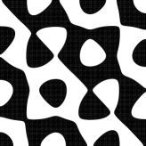
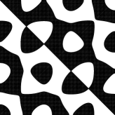
Figure 26. The graphs show nodal domains in the case $(p,q)=(8,3)$. From upper left to lower right, $\theta=0$, $\theta=2\pi/25$, $\theta=\theta_{1}\approx 0.57$, $\theta=19\pi/100$, $\theta=\theta_{13}\approx 0.61$, $\theta=\pi/5$, $\theta=\theta_{2}\approx 0.74$, $\theta=6\pi/25$ and $\theta=\pi/4$.

9. Table

$n$	$p$	$q$	$\lambda_{n}$	$n_{\text{ARot}}$	$n_{\text{SRot}}$	$n_{\text{AMir}}$	Comment
1	0	0	0		1		Courant sharp
2–3	1	0	1	1–2			Courant sharp
	0	1					—
4	1	1	2		2	1	Courant sharp
5–6	2	0	4		3–4		Courant sharp
	0	2					—
7–8	2	1	5	3–4			Lemma 3.1
	1	2					—
9	2	2	8		5		Courant sharp
10–11	3	0	9	5–6			Lemma 4.2
	0	3					—
12–13	3	1	10		6–7	2–3	Lemma 3.5
	1	3					—
14–15	3	2	13	7–8			Lemma 6.5
	2	3					—
16–17	4	0	16		8–9		Lemma 4.2
	0	4					—
18–19	4	1	17	9–10			Lemma 7.1
	1	4					—
20	3	3	18		10	4	Lemma 4.4
21–22	4	2	20		11–12		Lemma 6.2
	2	4					—
23–26	5	0	25	11–14			Lemma 3.1
	4	3					—
	3	4					—
	0	5					—
27–28	5	1	26		13–14	5–6	Lemma 3.5
	1	5					—
29–30	5	2	29	15–16			Lemma 3.1
	2	5					—
31	4	4	32		15		Lemma 4.4
32–33	5	3	34		16–17	7–8	Lemma 3.5
	3	5					—
34–35	6	0	36		18–19		Lemma 4.2
	0	6					—
36–37	6	1	37	17–18			Lemma 3.1
	1	6					—
38–39	6	2	40		20–21		Lemma 3.8
	2	6					—
40–41	5	4	41	19–20			Lemma 3.1
	4	5					—
42–43	6	3	45	21–22			Lemma 6.4
	3	6					—
44–45	7	0	49	23–24			Lemma 4.2
	0	7					—
46–48	7	1	50		22–24	9–11	Lemma 3.5
	5	5					—
	1	7					—
49–50	6	4	52		25–26		Lemma 6.6
	4	6					—
51–52	7	2	53	25–26			Lemma 3.1
	2	7					—
53–54	7	3	58		27–28	12–13	Lemma 3.5
	3	7				—
55–56	6	5	61	27–28			Lemma 3.1
	5	6					—
57–58	8	0	64		29–30		Lemma 4.2
	0	8					—
59–62	8	1	65	29–32			Lemma 3.1
	7	4					—
	4	7					—
	1	8					—
63–64	8	2	68		31–32		Lemma 3.3
	2	8					—
65	6	6	72		33		Lemma 4.4
66–67	8	3	73	33–34			Lemma 7.2
	3	8					—
68–69	7	5	74		34–35	14–15	Lemma 3.5
	5	7					—
70–71	8	4	80		36–37		Lemma 6.3
	4	8					—
72–73	9	0	81	35–36			Lemma 4.2
	0	9					—
74–75	9	1	82		38–39	16–17	Lemma 3.5
	1	9					—
76–79	9	2	85	37–40			Lemma 3.1
	7	6					—
	6	7					—
	2	9					—
80–81	8	5	89	41–42		18–19	Lemma 2.3
	5	8					—
82–83	9	3	90		40–41	20–21	Lemma 3.5
	3	9					—
84–85	9	4	97	43–44			Lemma 7.3
	4	9					—
86	7	7	98		42	22	Lemma 3.5
87–90	10	0	100		43–46		Lemma 3.3
	8	6					—
	6	8					—
	0	10					—
91–92	10	1	101	45–46			Lemma 3.1
	1	10					—
93–94	10	2	104		47–48		Lemma 3.8
	2	10					—
95–96	9	5	106		49–50	23–24	Lemma 2.3
	5	9					—
97–98	10	3	109	47–48			Lemma 3.1
	3	10					—
99–100	8	7	113	49–50			Lemma 2.3
	7	8					—
101–102	10	4	116		51–52		Lemma 7.4
	4	10					—
103–104	9	6	117	51–52			Lemma 2.3
	6	9					—
105–106	11	0	121	53–54			Lemma 4.2
	0	11					—
107–108	11	1	122		53–54	25–26	Lemma 3.5
	1	11					—
109–112	11	2	125	55–58			Lemma 3.1
	10	5					—
	5	10					—
	2	11					—
113	8	8	128		55		Lemma 2.3
114–117	11	3	130		56–59	27–30	Lemma 3.5
	9	7					—
	7	9					—
	3	11					—
118–119	10	6	136		60–61		Lemma 2.3
	6	10					—
120–121	11	4	137	59–60			Lemma 2.3
	4	11					—
122–123	12	0	144		62–63		Lemma 4.2
	0	12					—
124–127	12	1	145	61–64			Lemma 3.1
	9	8					—
	8	9					—
	1	12					—
128–129	11	5	146		64–65	31–32	Lemma 2.3
	5	11					—
130–131	12	2	148		66–67		Lemma 2.3
	2	12					—
132–133	10	7	149	65–66			Lemma 2.3
	7	10					—
134–135	12	3	153	67–68			Lemma 2.3
	3	12					—
136–137	11	6	157	69–70			Lemma 2.3
	6	11					—
138–139	12	4	160		68–69		Lemma 2.3
	4	12					—
140	9	9	162		70	33	Lemma 2.3
141–142	10	8	164		71–72		Lemma 2.3
	8	10					—
143–146	13	0	169	71–74			Lemma 3.1
	12	5					—
	5	12					—
	0	13					—
147–150	13	1	170		73–76	34–37	Lemma 3.5
	11	7					—
	7	11					—
	1	13					—
151–152	13	2	173	75–76			Lemma 2.3
	2	13					—
153–154	13	3	178		77–78	38–39	Lemma 2.3
	3	13					—
155–156	12	6	180		79–80		Lemma 2.3
	6	12					—
157–158	10	9	181	77–78			Lemma 2.3
	9	10					—
159–162	13	4	185	79–82			Lemma 3.1
	11	8					—
	8	11					—
	4	13					—
163–164	12	7	193	83–84			Lemma 2.3
	7	12					—
165–166	13	5	194		81–82	40–41	Lemma 2.3
	5	13					—
167–168	14	0	196		83–84		Lemma 4.2
	0	14					—
169–170	14	1	197	85–86			Lemma 2.3
	1	14					—
171–173	14	2	200		85–87		Lemma 2.3
	10	10					—
	2	14					—
174–175	11	9	202		88–89	42–43	Lemma 2.3
	9	11					—
176–179	14	3	205	87–90			Lemma 2.3
	13	6					—
	6	13					—
	3	14					—
180–181	12	8	208		90–91		Lemma 2.3
	8	12					—
182–183	14	4	212		92–93		Lemma 2.3
	4	14					—
184–185	13	7	218		94–95	44–45	Lemma 2.3
	7	13					—
186–189	14	5	221	91–94			Lemma 2.3
	11	10					—
	10	11					—
	5	14					—
190–193	15	0	225	96–99			Lemma 2.3
	12	9					—
	9	12					—
	0	15					—
194–195	15	1	226		95–96	46–47	Lemma 2.3
	1	15					—
196–197	15	2	229	99–100			Lemma 2.3
	2	15					—
198–199	14	6	232		97–98		Lemma 2.3
	6	14					—
200–201	13	8	233	101–102			Lemma 2.3
	8	13					—
202–203	15	3	234		100–101	48–49	Lemma 2.3
	3	15					—
204–205	15	4	241	103–104			Lemma 2.3
	4	15					—
206	11	11	242		102	50	Lemma 2.3
207–208	12	10	244		103–104		Lemma 2.3
	10	12					—
$\geq 209$			$\geq 245$				Proposition 2.1

10. Open problems

From the numerics together with our mathematical analysis for specific eigenspaces, it seems reasonable to correct some traveling folk conjecture into the following one:

Conjecture 10.1.

In a given eigenspace of dimension $2$, the maximal number of nodal domains is obtained for at least one eigenfunction $\Phi_{p,q}^{\theta}$ for some $\theta\in\{0,\frac{\pi}{4},\frac{\pi}{2},\frac{3\pi}{4},\pi\}$.

The numerical work of Corentin Léna [11] devoted to the analysis of spectral minimal partitions (showing non nodal $k$-minimal partitions starting from $k\geq 3$) suggests that there are only two Courant sharp situations. The case of the isotropic torus has finally been solved quite recently by C. Lena [12]. Following the strategy of Å. Pleijel [15], his proof is a combination of a lower bound (à la Weyl) of the counting function with an explicit remainder term and of a Faber–Krahn inequality for connected domains on the torus with an explicit upper bound on the area.

It is also natural to ask if there are similar results to the results concerning the Dirichlet problem on the square considered by A. Stern and Bérard–Helffer, that is the existence of an infinite sequence of eigenvalues such that a corresponding eigenfunction has only two nodal domains. We conjecture that it is impossible to find such a sequence. To justify this guess, one can try to show that in the Neumann case, the number of nodal lines touching the boundary tends to $+\infty$ as the eigenvalue tends to $+\infty$. This has a nice connection with a recent result of T. Hoffmann-Ostenhof [9], saying that the only eigenfunction whose nodal set does not touch the boundary is the constant one.

At the moment, we can only prove the following:

Proposition 10.2.

Let $(p,q)\in\mathbb{N}^{*}\times\mathbb{N}$ with $p>q$. Then, for any $\theta\in[0,\pi]$ the nodal lines of the eigenfunction $\Phi^{\theta}_{p,q}$ have at least $2p+2q$ touching points at the boundary.

We first prove the proposition, with the additional assumption that $\cos px$ and $\cos qx$ have no common zeros in $[0,\pi]$.

As we have seen in Subsection 5.2, the analysis of the zeros on the boundary is immediately related with the investigation of the solutions of

$$\cos px=t\cos qx\quad\text{or}\quad\cos py=t\cos qy$$

with $t=\pm\tan\theta$ or $t=\pm\frac{1}{\tan\theta}$. The result is then a consequence of the following lemma:

Lemma 10.3.

Let $(p,q)\in\mathbb{N}^{*}\times\mathbb{N}$ with $p>q$. Suppose that $\cos px$ and $\cos qx$ have no common zeros in $[0,\pi]$. Then, for any $t\in[-1,+1]$, the equation

$$\cos px=t\cos qx$$

has exactly $p$ solutions in $[0,\pi]$.

Proof.

We first observe that there are at most $p$ solutions. Indeed, if we choose $u=\cos x$ as new variable, we obtain a polynomial equation in the variable $u$ of degree $p$,

$$P_{p}(u)=tP_{q}(u)\,,$$

where $P_{p}$ is some Chebyshev polynomial defined by

$$\cos px=P_{p}(\cos x)\,.$$

Hence we get our first observation (counting with multiplicity).

We now show that there are at least $p$ solutions. For $t=0$, the solutions are the zeros of $x\mapsto\cos px$, that is

$$x_{k}^{(p)}=(2k+1)\frac{\pi}{2p}\,;\quad k=0,\dots,(p-1)\,.$$

The zeros $x_{\ell}^{(q)}$ ($\ell=0,\dots,q-1$) of $x\mapsto\cos qx$ will play an important role. We will indeed look at the function $f_{p,q}$ introduced in (5.5) and they correspond to vertical asymptotes of the graph of $f_{p,q}$.

For $t\neq 0$, say $t>0$, we have now to count the number of solutions of $f_{p,q}(x)=t$. First we observe that there is (at least) one solution in $(0,x_{0}^{(p)})$ and no solution in $(x_{p-1}^{(p)},\pi)$. Moreover $f_{p,q}$ is finite there.

We now consider the equation in the interval $I_{k}^{(p)}:=(x_{k}^{(p)},x_{k+1}^{(p)})$, for some $0\leq k\leq p-2$.

For a given interval there are three cases.

1. There is a zero $x_{\ell}^{(q)}$ in $I_{k}^{(p)}$. In this case the range of $f_{p,q}$ always contains $(0,+\infty)$ in particular there is always at least one point such that $f_{p,q}(x)=t$.

2. There are no zeros of $\cos qx$ in $I_{k}^{(p)}$ and $(-1)^{(k+1)}\cos qx>0$. We observe in this case that at $\hat{x}_{k}^{(p)}=(k+1)\frac{\pi}{p}$ which belongs to $I_{k}^{(p)}$, we have

   $$f_{p,q}(\hat{x}_{k}^{(p)})=(-1)^{k+1}/\cos(q\hat{x}_{k}^{(p)})\geq 1\,.$$ (10.1)

   We will see below that the inequality is strict when $p$ and $q$ are mutually prime. In the case when we have equality, we have $\sin(q\hat{x}_{k}^{(p)})=0$ and we get from (5.6) that we are at a local extremum of $f_{p,q}$.

3. There are no zeros of $\cos qx$ in $I_{k}^{(p)}$ and $(-1)^{(k+1)}\cos qx<0$. In this case the guess is that there are no zeros. We will get it at the end of the argument but the information is not needed for our lower bound.

To complete the lower bound we have simply to verify that for two intervals $I_{k}^{(p)}$, $I_{k+1}^{(p)}$ not containing a zero of $\cos qx$ we are either in a sequence case (2), case (3) or in a sequence case (3), case (2). This implies that we have for $|t|<1$ at least two solutions in the union of the two intervals. For $|t|=1$ the argument is the same if the inequality is strict in (10.1) and we have a double point if there is an equality (this will correspond to a critical point at the boundary).

If one of the intervals, say $I_{k+1}^{(p)}$, contains a zero of $\cos qx$, we play the same game as before but with the pair $I_{k}^{(p)}$, $I_{k+2}^{(p)}$.

Summing up we get the lower bound by $p$. Hence we have exactly $p$ zeros. ∎

Proof of Proposition 10.2 (with additional assumption).

We can now finish the proof of the proposition under the additional assumption that $\cos px$ and $\cos qx$ have no common zeros in $[0,\pi]$. The lemma can be applied (depending on $\theta$) either to $x=0$ and $x=\pi$ or to $y=0$ and $y=\pi$. For the two other cases, we can use that for $|t|>1$, $f_{p,q}(x)=t$ has at least one solution. ∎

Before attacking the general case, note the following lemma:

Lemma 10.4.

If $p$ and $q$ are mutually prime, and $0\leq k\leq p-2$,

$$(-1)^{k+1}\,\cos(q\hat{x}_{k}^{(p)})<1\,.$$

Proof.

Let us assume $k$ odd. We want to show that $\cos(k+1)\frac{q\pi}{p}\neq 1$. By contradiction, we would have

$$(k+1)\frac{q}{p}=2\ell\,.$$

This can be written in the form

$$\frac{(k+1)}{2}q=\ell p\,.$$

By assumption, $p$ and $q$ are mutually prime. This leads to $\ell=q\tilde{\ell}$, $\frac{k+1}{2}=p\tilde{\ell}$ for an integer $\tilde{\ell}$. We have now to remember that $\frac{k+1}{2}\in(\frac{1}{2},\frac{p-1}{2})$. This gives a contradiction.

Let us now assume $k$ even. We want to show that $\cos(k+1)\frac{q\pi}{p}\neq-1$. By contradiction, we would have

$$(k+1)q=(2\ell+1)p\,.$$

$p$ and $q$ being mutually prime. This leads to $k+1=\tilde{\ell}p$. This is again impossible because $1\leq(k+1)\leq p-1$. ∎

Remark 10.5.

This implies equality in all the lower bounds of the second part. This implies also $p-q-1$ local extrema in $(0,\pi)$ for $f_{p,q}$ as can be seen in Figures 17 and 22.

End of the proof of the general case..

We now explain how we can relax the assumption that $\cos px$ and $\cos qx$ (or equivalently $P_{p}$ and $P_{q}$) have no common zeros in $[0,\pi]$). A simple example is $p=3$ and $q=1$, where $x=\frac{\pi}{2}$ is a common zero of $\cos 3x$ and $\cos x$. This zero is common to the all family $x\mapsto\cos 3x-t\cos x$. Looking at $f_{3,1}(x)$, we observe that we can regularize it at $\frac{\pi}{2}$ and that it is enough to apply the previous argument for showing that there is at least two solutions of $f_{3,1}(x)=t$ for $|t|\leq 1$ (see Figure 27). This is of course trivial in this case.

Figure 27. The graph of the (regularized) $f_{3,1}$ in the interval $0<x<\pi$.

The general case is similar. We first determine the cardinal $p^{*}$ of the set $I^{*}_{p}$ in $\{1,\dots,p\}$) of the $k$’s such that $\hat{x}_{k}^{(p)}$ is a zero of $\cos qx$.

Similarly, we consider the set of the $\ell$ such that $\hat{x}_{k}^{(p)}=\hat{x}_{\ell}^{(q)}$ for some $k$. Another way of presentation is to claim the existence of a polynomial $Q$ of degree $p^{*}$ such that

$$P_{p}=Q\hat{P}_{p-p^{*}}\,,\,P_{q}=Q\hat{P}_{q-p^{*}}\,,$$

so that the regularization of $f_{p,q}$ is given by:

$$f_{p,q}(x)=\frac{\hat{P}_{p-p^{*}}(\cos x)}{\hat{P}_{q-p^{*}}(\cos x)}\,.$$

It suffices to do the same proof as before but keeping only in our construction the $x_{k}^{(p)}=x_{\ell}^{(q)}$ which are not the $p^{*}$ common zeros of $\cos px$ and $\cos qx$.

The proof is then identical and will give at least $p-p^{*}$ solutions of $f_{p,q}(x)=t$, hence of $P_{p}(x)-tP_{q}(x)=0$ in addition to the $p^{*}$ previously obtained. ∎

Proposition 10.6.

Let $(p,q)\in\mathbb{N}^{*}\times\mathbb{N}$ with $p>q$ and $\theta\in[0,\pi]$. Then the eigenfunction $\Psi:=\Phi^{\theta}_{p,q}$ satisfies

$$\mu(\Psi)\geq p+q+1\geq\sqrt{p^{2}+q^{2}}+1=\sqrt{\lambda}+1\,.$$ (10.2)

Proof.

This is obtained by using Euler’s formula, which implies (forgetting the contribution of the critical points inside the square)

$$\mu(\Psi)\geq b_{1}+\frac{1}{2}\#\{\mbox{boundary points}\}\,,$$

where $b_{1}$ is the number of connected components of $\partial\Omega\cup N(\Psi)$ ($N(\Psi)$ being the zero set of $\Psi$). Using $b_{1}\geq 1$ and Proposition 10.2 we get (10.2). ∎

This gives a rather explicit way to prove that for a specific family which seems relatively generic (any family corresponding to eigenvalues of multiplicity at most $2$) the number of nodal domains tends to $+\infty$. Hence we conjecture:

Conjecture 10.7.

For any sequence of eigenfunctions of the Neumann problem in the square associated with an infinite sequence of eigenvalues, the number of nodal domains tends to $+\infty$.

References

- [1] P. Bérard and B. Helffer. Dirichlet eigenfunctions of the square membrane: Courant’s property, and A. Stern’s and Å. Pleijel’s analyses. Preprint March 2014. ArXiv: 1402.6054.
- [2] P. Bérard and B. Helffer. A. Stern’s analysis of the nodal sets of some families of spherical harmonics revisited. Preprint July 2014. ArXiv: 1407.5564.
- [3] P. Bérard and B. Helffer. On the number of nodal domains of the 2D isotropic quantum harmonic oscillator– an extension of results of A. Stern– Preprint August 2014. ArXiv: 1409.2333
- [4] R. Courant. Ein allgemeiner Satz zur Theorie der Eigenfunktionen selbstadjungierter Differentialausdrücke. Nachr. Ges. Göttingen (1923), 81–84.
- [5] R. Courant and D. Hilbert. Methods of Mathematical Physics, Vol. 1. New York (1953).
- [6] G. Faber. Beweis, dass unter allen homogenen Membranen von gleicher Fläche und gleicher Spannung die kreisförmige den tiefsten Grundton gibt. S.-B. Math.-Nat. Kl. Bayer. Akad. Wiss. (1923), 169–172.
- [7] B. Helffer and T. Hoffmann-Ostenhof. Minimal partitions for anisotropic tori. J. Spectr. Theory 4 (2014), 221–233.
- [8] B. Helffer, T. Hoffmann-Ostenhof, and S. Terracini. Nodal domains and spectral minimal partitions. Ann. Inst. H. Poincaré Anal. Non Linéaire 26 (2009), 101–138.
- [9] T. Hoffmann-Ostenhof. Eigenfunctions for rectangles with Neumann boundary conditions. To appear in Moscow Math. Preprint arXiv:1301.7649.
- [10] E. Krahn. Über eine von Rayleigh formulierte Minimaleigenschaft des Kreises. Math. Ann. 94 (1924), 97–100.
- [11] C. Léna. Spectral minimal partitions for a family of tori. Preprint May 2014. Submitted.
- [12] C. Léna. Personal communication (October 2014).
- [13] J. Leydold. Knotenlinien und Knotengebiete von Eigenfunktionen. Diplom Arbeit, Universität Wien (1989), unpublished. Available at http://othes.univie.ac.at/34443/
- [14] J. Leydold. On the number of nodal domains of spherical harmonics. Topology 35 (1996), 301–321.
- [15] Å. Pleijel. Remarks on Courant’s nodal theorem. Comm. Pure. Appl. Math. 9 (1956), 543–550.
- [16] F. Pockels. Über die partielle Differentialgleichung and deren Auftreten in mathematischen Physik. Historical Math. Monographs. Cornell University. (1891) Available at https://archive.org/details/berdiepartiell02pockuoft.
- [17] I. Polterovich. Pleijel’s nodal theorem for free membranes. Proc. of the AMS 37 (3) (2009), 1021–1024.
- [18] A. Stern. Bemerkungen über asymptotisches Verhalten von Eigenwerten und Eigenfunctionen. Diss. Göttingen 1925.
- [19] A. Stern. Bemerkungen über asymptotisches Verhalten von Eigenwerten und Eigenfunctionen. Diss. Göttingen 1925. Extracts and annotations available at http://www-fourier.ujf-grenoble.fr/~pberard/R/stern-1925-thesis-partial-reprod.pdf.
- [20] J. Toth and S. Zelditch. Counting nodal lines that touched the boundary of an analytic domain. Journal of Differential Geometry 81 (2009), 649–686.
- [21] H. Weyl. über die asymptotische Verteilung der Eigenwerte, Nachrichten der Königlichen Gesellschaft der Wissenschaften zu Göttingen, (1911), 110–117.