Testing the maximal rank of the volatility process for continuous diffusions observed with noise
Abstract
In this paper, we present a test for the maximal rank of the volatility process in continuous diffusion models observed with noise. Such models are typically applied in mathematical finance, where latent price processes are corrupted by microstructure noise at ultra high frequencies. Using high frequency observations we construct a test statistic for the maximal rank of the time varying stochastic volatility process. Our methodology is based upon a combination of a matrix perturbation approach and pre-averaging. We will show the asymptotic mixed normality of the test statistic and obtain a consistent testing procedure.
Keywords: continuous Itô semimartingales, high frequency data, microstructure noise, rank testing, stable convergence.
AMS 2010 Subject Classification: 62M07, 60F05, 62E20, 60F17.
1 Introduction
In the last twenty years, asymptotic theory for high frequency data has received a great deal of attention in probability and statistics. This is mainly motivated by financial applications, where observations of stock prices are recorded very frequently. In an ideal world, i.e. under no-arbitrage conditions, price processes must follow an Itô semimartingale, which is a celebrated result of Delbaen and Schachermayer [4]. We refer to a monograph [8] for a comprehensive study of limit theorems for Itô semimartingales and their manifold applications in statistics.
Despite the aforementioned theoretical result, at ultra high frequencies, the financial data is contaminated by microstructure noise such as rounding errors, bid-ask bounces and misprints. One of the standard models for the microstructure noise is an additive i.i.d. process independent of the latent price (see e.g. [3, 14] among many others; an extension of this model can be found in [6]). More formally, the model is given as
| (1.1) |
where is a -dimensional continuous Itô semimartingale, and is a -dimensional i.i.d process independent of with
| (1.2) |
We are in the framework of infill asymptotics, i.e. while remains fixed. This paper is devoted to the test for the maximal rank of the co-volatility matrix of the unobserved diffusion process . We remark that this is an equivalent formulation of the following problem: What is the minimal amount of independent Brownian motions required for modeling the -dimensional diffusion ? Answering this question might give a direct economical interpretation of the financial data at hand. Furthermore, testing for the full rank of is connected to testing for completeness of financial markets.
In a recent paper [7], the described statistical problem has been solved in a continuous diffusion setting without noise (we also refer to an earlier article [5] for a related problem). The main idea is based upon a matrix perturbation method, which helps to identify the rank of a given matrix. The maximal rank of the stochastic co-volatility process is then asymptotically identified via a certain ratio statistic, which uses the scaling property of a Brownian motion. Clearly, the test statistic becomes invalid in the framework of continuous diffusion models observed with noise. To overcome this problem we apply the pre-averaging approach, which has been originally proposed in [6, 11]. As the name suggests, weighted averages of increments of the process are built over a certain window in order to eliminate the influence of the noise to some extent. This in turn gives the possibility to infer the co-volatility process . The size of the pre-averaging window is typically chosen as and objects as the integrated co-volatility can be estimated with the convergence rate of , which is known to be optimal.
At this stage, we would like to stress that combining the pre-averaging approach and the matrix perturbation method is by far not trivial. There are mainly two problems that need to be solved. First of all, when using the optimal window size of in the pre-averaging approach, the diffusion and the noise parts have the same order, and it becomes virtually impossible to distinguish the rank of the co-volatility from the unknown rank of the covariance matrix . Hence, we will choose a proper sub-optimal window size to still obtain a reasonable convergence rate for the test statistic. The second and more severe problem is that the ratio statistic proposed in [7] heavily relies on the scaling property of a Brownian motion. This scaling property is not shared by an i.i.d. noise process introduced in (1.2). Thus, a much deeper probabilistic analysis of the main statistic is required to come up with a valid testing procedure.
The paper is organized as follows. Section 2 gives the probabilistic description of the model, presents the main assumptions and defines the testing hypotheses. The background on matrix perturbation and pre-averaging method is demonstrated in Section 3. Section 4 presents the main results of the paper. Section 5 is concerned with a simulation study. All proofs are collected in Section 6.
2 The setting and main assumptions
We start with a filtered probability space , on which all stochastic processes are defined. As indicated at (1.1) we observe the -dimensional process at time points , . The process is given via
| (2.1) |
where is a -dimensional drift process, is a -valued volatility process and denotes a -dimensional Brownian motion. We introduce the notation
We need more structural assumptions on the processes and .
Assumption (A): The processes and have the form
| (2.2) | ||||
where and are -valued, , and are -valued, and are -valued, and is -valued, all those processes being adapted. Finally, the processes are càdlàg and the processes are locally bounded.
Notice that (A) is exactly the same assumption, which has been imposed in [7]. We remark that, by enlarging the dimension of the Brownian motion if necessary, we may assume without loss of generality that all processes are driven by the same Brownian motion. In the framework of a stochastic differential equation, i.e. when and , assumption (A) is automatically satisfied whenever and (due to Itô’s formula). We also remark that assumption (A) is rather unusual in the literature. Indeed, for classical high frequency statistics, such as e.g. power variations (cf. [2]), only the first line of (2.2) is required. However, when our test statistic, which will be introduced in Section 4, turns out to be degenerate and, in contrast to classical cases, we require a higher order stochastic expansion of the increments of . This explains the role of the second and third line of (2.2). Finally, we specify our assumptions on the noise process introduced at (1.2).
Assumption (E): The i.i.d. process is -adapted and independent of , , , , , , hence also independent of , and . Furthermore, it is Gaussian, meaning that and for all with .
Remark 2.1.
Theoretically, we could discuss a more general structure of the noise. In particular, we could give up the assumption of the Gaussianity. What we really require is the mutual independence of the noise at different times as well as the existence of the moments up to a certain order. Also the independence assumption between the noise and the semimartingale could be generalized; see e.g. [6, 10] for an exposition of the details.
Now, for any , we introduce the following subsets of :
| (2.3) |
Notice that the sets and are indeed -measurable. This can be justified as follows. The rank is the biggest integer such that the sum of the determinants of the matrices , where runs through all subsets of with points, is positive; see e.g. [5, Lemma 3]. Since the mapping is continuous by assumption (A), this implies that for any the random set is open in , so the mapping is lower semi-continuous. The very same argument proves that the random set
is non-empty and open for each . Hence, this set has a positive Lebesgue measure, which helps to statistically identify the maximal rank (in contrast to lower ranks , which might be attained at a single point on the interval ).
The following discussion is devoted to testing the null hypothesis against the alternative (or against ). Notice that this a pathwise hypothesis, since we test whether a given path belongs to (or ) or not. It is in general impossible to know whether this hypothesis holds for another path .
3 Matrix perturbation and pre-averaging approach
3.1 Matrix perturbation method
The matrix perturbation method is a numerical approach to the computation of the rank of a given matrix. It has been introduced in [7] in the context of rank testing. To explain the main idea of our method, we need to introduce some notation. Recall that and are the dimensions of and , respectively. Let denote the set of all matrices and , , the set of all matrices in with rank . Furthermore, let be the set of all matrices. For any matrix we denote by the th column of ; for any vectors in , we write mat for the matrix in whose th column is the column vector . For and we define the quantity
In other words, is the set of all matrices with columns equal to those of and the remaining ones equal to those of (all of them being at their original places). We also define the number
| (3.1) |
We demonstrate the main ideas of the matrix perturbation approach for a deterministic problem first. Let be an unknown matrix with rank . Assume that, although is unknown, we have a way of computing for all and some given matrix . The multi-linearity property of the determinant implies the following asymptotic expansion
| (3.2) |
This expansion is the key to identification of the unknown rank . Indeed, when we deduce that
| (3.3) |
However, it is impossible to choose a matrix which guarantees for all . To solve this problem, we can use a random perturbation. As it has been shown in [7], for any we have almost surely when is the random matrix whose entries are independent standard normal (in fact, the random variable has a Lebesgue density). This is intuitively clear, because the multivariate standard normal distribution does not prefer directions. It is exactly this idea which will be the core of our testing procedure.
3.2 Pre-averaging approach
In this subsection, we briefly introduce the pre-averaging method; we refer to e.g. [6, 11] for a more detailed exposition.
Let be a weight function with , which is continuous, piecewise with piecewise Lipschitz derivative and . A canonical choice of such a function is given by ; see [6] for its interpretation. Now, let be a sequence of positive integers representing the window size such that and . For any stochastic process , we define the pre-averaged increments via
| (3.4) |
where . Roughly speaking, this local averaging procedure reduces the influence of the noise process when we apply it to the noisy diffusion process defined at (1.1). Indeed, we may show that
where the first approximation is essentially justified by the independence of the increments of and the first identity of (3.4), and the second approximation follows from the i.i.d. structure of the noise process and the second identity of (3.4). We clearly see that a large increases the influence of the diffusion part and diminishes the influence of the noise part . However, in standard statistical problems, e.g. estimation of quadratic variation, the optimal rate of convergence is obtained when the contributions of both terms are balanced. This results in the choice of the window size with , where . With this window size we deduce for instance that
where the constants and are defined by
(cf. [6]). The bias can be corrected via
and the statistic becomes a consistent estimator of the quadratic covariation of with convergence rate . This rate is known to be optimal.
As explained in the introduction, the optimal choice of the window size as introduced above would not lead to a feasible testing procedure for the maximal rank . Due to the complex structure of the test statistic, which will be introduced in Section 4, there is no de-biasing procedure as above (when there are no further restrictions on the rank of the covariance matrix ). For this reason we introduce the following window size :
| (3.5) |
Within the framework of our test statistic, this choice of leads to an optimal rate of convergence, which becomes (although better rates of convergence are theoretically possible when using alternative test statistics). We show the intuition behind this choice in the next section. We remark that an easier choice of the window size would be , which would completely eliminate the influence of the noise process on the central limit theorem. However, this would lead to a slower rate of convergence . For this reason we dispense with the exact exposition of this case.
4 Main results
4.1 Test statistic
In this subsection, we introduce a random perturbation of the original data and define the main statistics. Following the basic ideas of [7] and the motivation of Subsection 3.1, we define a -dimensional ‘perturbation’ process by
where is a positive definite deterministic matrix and is a -dimensional Brownian motion. Without loss of generality, we may assume that is also defined on the filtered probability space . Let be the sub--algebra, which is generated by all processes appearing in (A) and by the noise process . We assume that is independent of . Now, we use to define the perturbed process
| (4.1) |
where and the sequence is defined at (3.5). In some sense, the perturbation process plays the role of the random perturbation matrix introduced after (3.3). As we will see below, our two main statistics will be constructed at two different frequencies and , which will be indicated by the constant .
Recall the definition of the pre-averaged quantity introduced in (3.4) for a stochastic process . We sometimes write instead of if we want to stress the dependency of the term on the weight function . Furthermore, we use the notation to indicate that the quantity is built using frequency with , i.e.
| (4.2) |
If defined at (4.1), we will slightly abuse the notation introduced in (4.2) and use the convention . Now, we define our main test statistics via
| (4.3) |
for with the test function on given as
| (4.4) |
Note that the summands in (4.3) use non-overlapping increments of the process , and also the statistics and are based on distinct increments.
Remark 4.1.
The statistic is similar in spirit to the one introduced in [7], where a -dimensional continuous Itô semimartingale without noise has been considered. Therein, the statistics defined in [7, Equation (2.13)], which use the raw increments instead of pre-averaged ones, satisfy the following law of large numbers
This should be compared with the motivation described at (3.3). The latter convergence asymptotically identifies the maximal rank . The crucial difference to our framework is that this convergence is no longer valid when we use the statistics introduced in (4.3). It relies on the fact that the noise process does not have the scaling property of the driving Brownian motion . To overcome this issue, we will not only use different frequencies and , but also two different weight functions and , which are connected through certain identities. For this purpose a very thorough analysis of the asymptotic behaviour of is required.
Remark 4.2.
Let us explain the choice of the window size introduced at (3.5) and the perturbation rate . Under assumptions (A) and (E) we will prove the following asymptotic decomposition for
| (4.5) | ||||
where the -valued sequences and are tight. The matrix , which is the dominating term in the expansion, is defined by
while depends on introduced in (2.2), comes solely from the perturbation and is associated with the noise process (the third order term is connected to and the term depends on , defined in (2.2)). Since whenever , our statistic is degenerate in the sense that the second order term enters the law of large numbers. At this stage, we realize that the choice of the window size and the perturbation rate creates a balance between the second order term in the stochastic expansion coming from the diffusion process, the noise process and the perturbation process . The classical choice would make the noise part one of the dominating terms, but in this case, the estimation of the maximal rank would be virtually impossible since we impose no assumptions on the covariance matrix of the noise. On the other hand, when the noise part would enter the third order term and thus would not influence the limit theory. Although the asymptotic results become much easier in the latter case, the convergence rate gets rather low (). Hence, within the framework of our test statistic, the choice meets the balance between feasibility of the testing procedure and the optimal rate of convergence.
Clearly, plays the role of the perturbation matrix defined in section 3.1 while . Since it is impossible to guarantee that the matrices and have full rank, we require the presence of the matrix to insure almost sure invertibility of the sum. Thus, the perturbation process plays the role of regularization.
4.2 Notation
In order to state the limit theory for the statistics , we need to introduce some notation. For any weight function we define the quantities
| (4.6) | |||||
For , we define the function on by
| (4.7) |
where was introduced at (3.1). Let and be Brownian motions of dimension and , respectively, and let be a i.i.d. sequences of -dimensional standard normal random variables. , , and are defined on some filtered probability space and are assumed to be independent. Let be the space of all symmetric positive-semidefinite matrices . We introduce the space , and let . By we denote the matrix root of .
Now, for , we define the -dimensional variables (explicitly writing the components with )
| (4.8) | ||||
| (4.9) | ||||
Some explanations are in order to understand these definitions.
Remark 4.3.
To get an intuition for the notation we remark that the components of account for the processes in assumption (A) that will appear in the limit. This means that is related to , to , to and to . Finally, accounts for the covariance structure of the noise and is associated with . As motivated above we use different rates in our procedure. Therefore, we also have to define the limit for the two cases .
Remark 4.4.
Note that the random-vectors and are uncorrelated whenever .
Using the notation at (4.7), we define for a weight function , and the real-valued random variables
and set
| (4.10) | ||||
Remark 4.5.
Under the special assumption that (which corresponds to the situation without noise), the sequences and have the same global law which implies also that and . This is not the case when . Proposition 4.9 will demonstrate under which conditions one can find another weight function such that and even in the general situation that .
Remark 4.6.
We have introduced the random variables only for weight functions, implying that is continuous and piecewise with a piecewise Lipschitz derivative . As a matter of fact, we will often work with a discretized version of defined as
| (4.11) |
Note that and that converges to uniformly on . By definition, fails to be a weight function as it is not continuous. Nevertheless, the integrals , and still make sense. This corresponds to the fact that introduced at (4.6) is well-defined for . Moreover, we have by a Riemann approximation argument that
For , we must approximate the derivative and set
| (4.12) |
where the second identity follows again by a Riemann approximation argument. With this convention, we can extend the notation and write , , and , respectively.
4.3 Law of large numbers
In this subsection, we present the law of large numbers for the statistic . The quantity defined at (4.10) will essentially determine the limit. First, we demonstrate how the terms and depend on the rank of the argument . The following lemma has been shown in [7, Lemma 3.1].
Lemma 4.7.
Let with and be a weight function. Then, if and , we deduce that
| (4.13) | ||||
| (4.14) |
The law of large numbers is as follows.
Theorem 4.8.
Assume that conditions (A) and (E) hold. Let and be a weight function. Then, on and for , we obtain the convergence
| (4.15) |
In view of Remark 4.1, Theorem 4.8 is not directly applicable since the limit crucially depends on , meaning that generally . In particular, the ratio statistics does not contain any information about the unknown maximal rank . To make use of Theorem 4.8 we need a better understanding of the structure of the functional . The following proposition is absolutely crucial for our testing procedure.
Proposition 4.9.
(i) Fix , and . Then there exist -functions such that
| (4.16) |
for any weight function .
(ii) Let and be weight functions such that and for .
Then, for any and any , we obtain that
Proposition 4.9(i) says that the quantity does not depend on the entire function , but only on the quantities , . But most importantly, Proposition 4.9(ii) and Theorem 4.8 imply the convergence
| (4.17) |
whenever the pair of weight functions satisfies the conditions of Proposition 4.9(ii). This opens the door to hypothesis testing. We now give an example of a pair of weight function which fulfills the conditions of Proposition 4.9(ii).
Example 4.10.
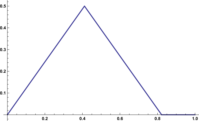
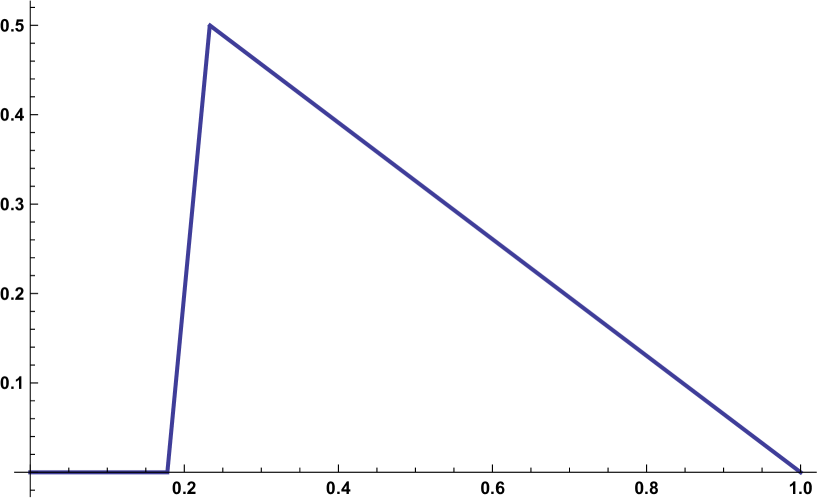
Remark 4.11.
From a statistical point of view and regarding the definition of the pre-averaged increments in (3.4), we see that it is certainly not ideal to chose weight functions which are locally constant. Nevertheless, Example 4.10 is an attempt to reduce the parts where the weight functions are constant while still sticking to a rather simple ‘triangular’ form.
4.4 Central limit theorem and testing procedure
In order to provide a formal testing procedure associated with the convergence in probability at (4.17) we need to show a joint stable central limit theorem for the statistics . We say that a sequence of random variables converges stably in law to (), where is defined on an extension of the original probability space , if and only if
for any bounded and continuous function and any bounded -measurable random variable . We refer to [1], [9] or [12] for a detailed study of stable convergence. Note that stable convergence is a stronger mode of convergence than weak convergence, but it is weaker than convergence in probability.
Now, let and be two weight functions satisfying the conditions of Proposition 4.9(ii). We define the statistic via
| (4.18) |
The following theorem is one of the most important results of the paper.
Theorem 4.12.
Assume that conditions (A) and (E) are satisfied, the weight functions fulfill the assumptions of Proposition 4.9(ii) and for some . Then we obtain the stable convergence
| (4.19) |
where
| (4.20) |
is a diagonal matrix. denotes the two dimensional mixed normal distribution with -conditional mean and -conditional covariance matrix .
Note that the rate of convergence corresponds to for our choice of the window size at (3.5). We remark that due to Proposition 4.9(ii), we know that such that the same centering term appears in both components on the right-hand side of (4.18). Again thanks to Proposition 4.9(ii) we see that the two diagonal elements of coincide. In order to obtain a feasible version of the stable convergence in (4.19), we need to construct a consistent estimator of the -conditional covariance matrix . To this end, we define the following estimators for the ‘second moments’:
| (4.21) | ||||
| (4.22) | ||||
| (4.23) | ||||
where is given at (4.4). Following the intuition from (4.17) we define an estimator via
| (4.24) |
Now, we obtain the following proposition.
Proposition 4.13.
Assume that conditions (A) and (E) are satisfied and the weight functions fulfill the assumptions of Proposition 4.9(ii).
(i) Let . Then, on :
| (4.25) | ||||
| (4.26) | ||||
| (4.27) |
(ii) We have the (stable) central limit theorem
| (4.28) |
where is defined on an extension of the original probability space and is independent of the -algebra . The random variable is defined via
| (4.29) |
We remark that Proposition 4.13(ii) follows directly from Theorem 4.12, Proposition 4.13(i) and the delta method for stable convergence. For this, it is essential to realize that, even though the estimator for the conditional variance is not -measurable, it converges to a -measurable limit due to Proposition 4.13(i) and Theorem 4.8.
Notice also that due to Proposition 4.9(ii) the right-hand side of (4.25) and (4.26) coincide and, moreover, that the right-hand side of (4.27) can be written as
Remark 4.14.
The feasible central limit theorem at (4.28) opens the door to hypothesis testing. Let us define the rejection regions via
| (4.33) | ||||
| (4.34) |
where denotes the -quantile of the standard normal distribution. Obviously, the rejection region corresponds to vs. , while corresponds to vs. . The asymptotic level and consistency of the test are demonstrated in the following corollary.
Corollary 4.15.
Assume that conditions (A) and (E) are satisfied and the weight functions fulfill the assumptions of Proposition 4.9(ii).
(i) The test defined through (4.33) has asymptotic level in the sense that
| (4.35) |
Furthermore, the test is consistent, i.e.
| (4.36) |
(ii) The test defined through (4.34) has asymptotic level at most in the sense that
| (4.37) |
Furthermore, the test is consistent, i.e.
| (4.38) |
5 Simulations
In this section, we want to examine how well the testing procedure for the maximal rank performs in finite samples. The main focus lies on considering the convergence results in (4.28), (4.35) and (4.36). Complementing these results, we examine how well the estimator works to estimate the maximal rank (using the law of large numbers which is implicitly given by (4.28)). To this end, we consider the integer-valued modification of defined as
| (5.1) |
We emphasize that due to the rate of convergence of we expect a worse performance in finite samples in comparison to the simulation study in [7] (there, the rate of convergence is ).
5.1 Results
All processes are simulated on the interval and we use four different frequencies , , and . We remark that even the highest frequency is nowadays available for liquid assets. Following the simulation study in [7], we set and due to [6] we use for the pre-averaging procedure. This results in window sizes of , , and , respectively. We use the weight functions explicitly constructed in Example 4.10. We perform 500 repetitions to uncover the finite sample properties. The following quantities are reported
-
•
the sampling frequency;
-
•
the number of big blocks;
-
•
the first four moments of the test statistic defined at (4.28) to check for the normal approximation;
-
•
the proportion of rejection for the possible null hypotheses with defined at (2.3) at level ;
-
•
the proportion of the event that the estimator defined at (5.1) coincides with .
We conduct the simulation study for the cases . For each of them, we examine different models for the semimartingale . We are interested in how robust our testing procedure is with respect to a violation of assumption (A). This can be seen in case 3, respectively, where the volatility is not continuous. For the noise part, we always assume the covariance structure of .
5.1.1
We consider the following four models:
-
(i)
Model 1: We have vanishing drift and constant volatility , implying .
-
(ii)
Model 2: We observe pure noise, so and , implying .
-
(iii)
Model 3: We have a constant drift of and a volatility of , implying .
-
(iv)
Model 4: We have a drift of and a volatility of , implying .
The results for the four models are summarized in the following table according to their order:
| 1st mt | 2nd mt | 3rd mt | 4th mt | |||||
|---|---|---|---|---|---|---|---|---|
| 21 | -0.134 | 1.460 | -0.363 | 6.567 | 0.378 | 0.106 | 0.734 | |
| 46 | -0.075 | 1.268 | -0.579 | 5.343 | 0.652 | 0.084 | 0.862 | |
| 100 | -0.036 | 1.089 | -0.153 | 3.665 | 0.934 | 0.068 | 0.950 | |
| 215 | -0.068 | 1.097 | -0.079 | 3.932 | 0.998 | 0.060 | 0.990 | |
| 21 | -0.056 | 1.403 | -0.403 | 6.206 | 0.096 | 0.454 | 0.790 | |
| 46 | 0.020 | 1.323 | 0.171 | 5.998 | 0.084 | 0.672 | 0.860 | |
| 100 | 0.006 | 1.129 | 0.168 | 3.913 | 0.062 | 0.926 | 0.952 | |
| 215 | -0.016 | 1.024 | -0.039 | 3.536 | 0.048 | 1.000 | 0.992 | |
| 21 | -0.252 | 2.018 | -2.222 | 17.611 | 0.298 | 0.132 | 0.664 | |
| 46 | -0.050 | 1.364 | -0.477 | 6.220 | 0.484 | 0.092 | 0.802 | |
| 100 | -0.140 | 1.105 | -0.427 | 3.596 | 0.708 | 0.076 | 0.878 | |
| 215 | -0.026 | 1.013 | -0.159 | 3.100 | 0.940 | 0.054 | 0.966 | |
| 21 | -0.373 | 1.959 | -3.042 | 15.488 | 0.310 | 0.154 | 0.684 | |
| 46 | -0.231 | 1.389 | -1.271 | 6.902 | 0.484 | 0.076 | 0.788 | |
| 100 | -0.115 | 1.080 | -0.489 | 3.475 | 0.808 | 0.058 | 0.912 | |
| 215 | -0.048 | 0.985 | -0.257 | 3.129 | 0.986 | 0.052 | 0.982 |
5.1.2
We consider the following four models:
-
(i)
Model 1: We have vanishing drift and constant volatility , implying .
-
(ii)
Model 2: We have pure noise, so .
-
(iii)
Model 3: We have a drift of , and a volatility of , implying .
-
(iv)
Model 4: We have a drift of , and a volatility of
, implying .
The results for the four models are summarized in the following table according to their order:
| 1st mt | 2nd mt | 3rd mt | 4th mt | ||||||
|---|---|---|---|---|---|---|---|---|---|
| 10 | -0.146 | 2.836 | -1.952 | 33.933 | 0.524 | 0.264 | 0.226 | 0.616 | |
| 23 | -0.034 | 1.892 | -0.119 | 13.661 | 0.690 | 0.336 | 0.140 | 0.678 | |
| 50 | -0.033 | 1.379 | -0.081 | 5.987 | 0.890 | 0.448 | 0.088 | 0.774 | |
| 107 | -0.059 | 1.238 | -0.263 | 4.451 | 0.992 | 0.626 | 0.078 | 0.842 | |
| 10 | -0.097 | 3.839 | -15.410 | 297.391 | 0.212 | 0.316 | 0.558 | 0.646 | |
| 23 | -0.074 | 2.054 | -0.181 | 24.391 | 0.130 | 0.328 | 0.720 | 0.716 | |
| 50 | 0.113 | 1.357 | 0.775 | 6.365 | 0.104 | 0.390 | 0.926 | 0.780 | |
| 107 | -0.066 | 1.290 | -0.274 | 4.658 | 0.084 | 0.672 | 0.992 | 0.882 | |
| 10 | -0.293 | 3.747 | -0.119 | 101.560 | 0.288 | 0.246 | 0.388 | 0.286 | |
| 23 | -0.388 | 1.916 | -1.635 | 11.157 | 0.236 | 0.156 | 0.428 | 0.346 | |
| 50 | -0.090 | 1.251 | -0.396 | 4.483 | 0.424 | 0.090 | 0.482 | 0.590 | |
| 107 | -0.152 | 1.214 | -0.501 | 4.777 | 0.602 | 0.082 | 0.704 | 0.740 | |
| 10 | -0.062 | 3.308 | -6.196 | 88.100 | 0.294 | 0.206 | 0.304 | 0.260 | |
| 23 | -0.279 | 2.020 | -2.432 | 17.677 | 0.246 | 0.162 | 0.386 | 0.418 | |
| 50 | -0.061 | 1.438 | -0.481 | 6.609 | 0.434 | 0.098 | 0.450 | 0.522 | |
| 107 | 0.008 | 1.148 | -0.123 | 4.544 | 0.668 | 0.058 | 0.678 | 0.756 |
5.1.3
We consider the following four models:
-
(i)
Model 1: We have vanishing drift and constant volatility . Hence, the maximal rank is .
-
(ii)
Model 2: We have pure noise, so .
-
(iii)
Model 3: We have a drift of , and a volatility of , implying .
-
(iv)
Model 4: We have a drift of , and a volatility of
, implying .
The results for the four models are summarized in the following table according to their order:
| 1st mt | 2nd mt | 3rd mt | 4th mt | |||||||
|---|---|---|---|---|---|---|---|---|---|---|
| 7 | -0.291 | 4.854 | -11.705 | 195.934 | 0.622 | 0.460 | 0.344 | 0.326 | 0.556 | |
| 15 | -0.041 | 2.631 | -1.521 | 37.908 | 0.764 | 0.538 | 0.288 | 0.192 | 0.636 | |
| 33 | 0.057 | 1.844 | -0.258 | 10.721 | 0.930 | 0.692 | 0.368 | 0.146 | 0.702 | |
| 71 | 0.014 | 1.459 | 0.116 | 6.382 | 0.988 | 0.870 | 0.414 | 0.098 | 0.776 | |
| 7 | -0.177 | 5.507 | -9.964 | 221.460 | 0.318 | 0.370 | 0.500 | 0.674 | 0.594 | |
| 15 | 0.017 | 2.779 | 2.579 | 59.508 | 0.174 | 0.314 | 0.570 | 0.792 | 0.652 | |
| 33 | 0.023 | 1.565 | -0.003 | 7.529 | 0.122 | 0.308 | 0.708 | 0.940 | 0.706 | |
| 71 | -0.035 | 1.507 | -0.340 | 6.874 | 0.100 | 0.452 | 0.860 | 0.990 | 0.754 | |
| 7 | -0.365 | 5.509 | -11.808 | 413.241 | 0.294 | 0.278 | 0.378 | 0.562 | 0.202 | |
| 15 | -0.282 | 2.392 | -1.297 | 21.282 | 0.264 | 0.184 | 0.344 | 0.660 | 0.288 | |
| 33 | -0.333 | 1.701 | -1.506 | 8.125 | 0.254 | 0.130 | 0.418 | 0.818 | 0.392 | |
| 71 | -0.074 | 1.279 | 0.026 | 5.215 | 0.446 | 0.074 | 0.502 | 0.948 | 0.574 | |
| 7 | -0.238 | 9.259 | 70.679 | 2873.157 | 0.470 | 0.368 | 0.348 | 0.440 | 0.190 | |
| 15 | -0.082 | 3.063 | -3.513 | 56.660 | 0.560 | 0.320 | 0.212 | 0.340 | 0.246 | |
| 33 | -0.137 | 1.762 | -0.736 | 9.407 | 0.644 | 0.292 | 0.140 | 0.362 | 0.380 | |
| 71 | -0.054 | 1.683 | -0.691 | 8.858 | 0.848 | 0.412 | 0.128 | 0.430 | 0.494 |
5.2 Summary
According to our theoretical results, the empirical counterpart of the first four moments, level and power seem to converge to their theoretical analogues as . However, the speed of convergence depends on the particular model and the dimension .
First, we observe that higher moments seem to converge much slower than lower moments. An extreme example is , Model 4, where the simulated fourth moment equals at frequency . This effect appears to be stronger for higher dimensions. It can be explained by the fact that the true rate of convergence is rather than , which decreases when is growing. Furthermore, there are several small order terms in the expansion of the main statistic, which seem to influence the finite sample performance at relatively low frequencies. This is confirmed by the observation that we get the best simulation results for constant volatility and vanishing drift, where these lower order terms do not appear.
The approximation of power again depends on the complexity of time-varying coefficients of the model and the dimension . Quite intuitively, we observe a better power performance for alternative hypotheses, which are more distant to the true one. For instance, for and Model 1, where the maximal rank is 3, the simulated powers for , and at frequency are , and , respectively. Finally, we remark that, although Model 3 () does not satisfy our assumptions since the volatility process is not continuous, the power and level performance is well comparable with other simulated models.
6 Proofs
Before presenting the proofs in detail, let us briefly outline the roadmap of this section. In Subsection 6.1 we introduce some technical results about expansions of determinants. We justify the asymptotic expansion at (3.2) and also show some more involved results.
In Subsection 6.2, we show that – using a standard localization procedure – we obtain the stochastic decomposition explained in Remark 4.2. Moreover, we show how the law of the dominating term in the expansion can be expressed in terms of the notation introduced in Subsection 4.2.
Subsection 6.3 is especially concerned with the proof of Proposition 4.9. To this end, we perform a very detailed analysis of the terms and introduced at (4.10) and their dependency on the weight function . This mainly relies on an application of the Leibniz rule for the calculation of the determinants and a repeated use of the Itô isometry to calculate the expectations.
Subsection 6.4 deals with the proof of the main Theorem 4.12 and of Proposition 4.13. First, we show that – thanks to the stochastic expansion established in Subsection 6.2 – the main approximation idea motivated in Subsection 3.1 works in the stochastic setting. The second main step in the proof of Theorem 4.12 is the application of a stable central limit theorem for semimartingales (see e.g. [9, Theorem IX.7.28 ]). Proposition 4.13(i) follows along the lines of parts of the proof of Theorem 4.12. Proposition 4.13(ii) follows by Theorem 4.12, Theorem 4.8 – which in tern is a direct consequence of Theorem 4.12 – and Proposition 4.13(ii) by applying the delta method for stable convergence. Note that this procedure does only work under a proper choice of the pair of weight functions which fulfills Proposition 4.9(ii).
The proof of Corollary 4.15 is essentially a consequence of the stable convergence at (4.28) and is referred to Subsection 6.5.
6.1 Expansion of determinants
Due to Subsection 3.1, the key to identifying the unknown rank of a matrix is the matrix perturbation method which results in the expansion at (3.2). While we could show the law of large numbers at (4.15) with an expansion like the one at (3.2), we need a higher order expansion of the determinant to derive the central limit theorem at (4.19). Therefore, we shall introduce some additional notation to the one in Subsection 3.1 which is similar to the one introduced in [7].
In the sequel, denotes the Euclidean norm of a matrix . For any positive integer we denote with the set of all multi-integers with and , and the set of all partitions of such that contains exactly points. For , and , we call the matrix in whose th column is the th column of when .
Due to the multi-linearity property of the determinant we have the following identity for all
| (6.1) |
For and , recalling (3.1), we recover the identity
| (6.2) |
and set
| (6.3) |
with the convention that and . Let and . Using (6.1) we obtain the asymptotic expansion
| (6.4) | ||||
This observation gives rise to the following lemma (see also [7, Lemma 6.2]).
Lemma 6.1.
There is a constant such that for all , all and all with we have with
| (6.5) |
| (6.6) |
If further , with and , then
| (6.7) |
6.2 The stochastic decomposition
Under assumption (A) and by a standard localization procedure (see e.g. [2, Section 3]), it is no restriction to make the following technical assumption.
Assumption (A1): Assumption (A) holds and the processes , , , , , , , , defined at (2.1) and (2.2) are uniformly bounded in .
We make the convention that all constants are denoted by , or if they depend on an additional parameter . The constants never depend on . To ease notation, we use generic constants that may change from line to line. We introduce the filtration defined as
where is the -field generated by the whole process . For any process and for the filtrations , and , we will use the simplifying notation
| (6.8) |
Note that we have the ‘nesting property’ and , respectively. Now, we show that under (A) we can obtain the stochastic decomposition at (4.5) explained in Remark 4.2. To do so, we notice (see [7, Section 6]) that under (A), and for any , we have the following expansion for the increment (using vector notation):
where
| (6.9) | |||||
By the Burkholder-Gundy inequality (see e.g. [13]) we have under (A1) for all and for that
| (6.10) |
We set
Using the Burkholder-Gundy inequality and Hölder inequality leads to (recall that )
| (6.11) |
Let be a weight function (see Subsection 3.2) and its discretization introduced at (4.11). For we define the function
Using (6.9) with with and we then obtain the stochastic decomposition at (4.5), namely
where (using vector notation)
and is the remainder term. In the sequel, we will make the convention that . With the following lemma, we can deduce that under assumption (A1) the -valued sequences are tight (see also equation (6.15) in [7]).
Lemma 6.2.
Let the assumptions (A1) and (E) be statisfied. For there is a such that we have the following estimates
Proof.
Lemma 6.3.
Assume (A1) and (E). Then .
Proof.
The proof follows along the lines of the proof of Lemma 6.3 in [7].
Lemma 6.4.
Let the assumptions (A1) and (E) be satisfied. Fix a weight function . Then, for any , and the -conditional law of
coincides with the -conditional law of
where
| (6.12) |
Proof.
As a direct consequence of Lemma 6.4 we can deduce that
| (6.13) | ||||
| (6.14) |
6.3 Proof of Lemma 4.7 and Proposition 4.9
Proof of Lemma 4.7.
Proof of Proposition 4.9.
We start with the proof of part (i). Let , , and be any weight function. Using the notation at (4.8) and (4.9), we define the matrices
being elements of . Furthermore, for we will use the notation
Then, developing the determinant with the Leibniz rule, we obtain the identity
| (6.15) | ||||
where denotes the group of all permutations of the set and is the sign of the permutation . The last step in the computation is due to the fact that the vectors and are uncorrelated if . Thus, for fixed and , the mapping can be considered as a polynomial in variables of the form
| (6.16) |
where , and . Using Itô’s isometry, (6.16) takes one of the following three forms with :
Hence, if we additionally fix , then there is a polynomial such that the mapping can be written as
This shows the first part of (4.16). To show the second part, we use the relationship
By a similar calculation as in (6.15) we obtain that
If we fix again and , the mapping can be considered as a polynomial in variables of the form
| (6.17) |
where , and . By a careful calculation, we can see that (6.17) takes one of the following five forms with :
We remark that the constants do not depend on . Consequently, if we additionally fix , there is a polynomial such that the mapping can be written as
which proves part (i) of Proposition 4.9. By an inspection of the previous calculations, we see that the only term where appears is the term . Hence, for any , , we have
This shows part (ii) of Proposition 4.9.
6.4 Proof of Theorem 4.12 and Proposition 4.13
Let be a weight function. We begin by constructing approximations for the main test statistics defined at (4.3) and given at (4.21), (4.22) and (4.23). The approximations are discretized versions of (see (4.15)) and the right-hand sides of (4.25) to (4.27)
| (6.18) |
The lemma is based on the asymptotic expansion at (6.4).
Lemma 6.5.
Assume (A1), (E), let , and be two weight functions (not necessarily satisfying the conditions of Proposition 4.9(ii)). Then, on , we have that
| (6.19) | |||
| (6.20) |
Proof.
The proof is an adaption of the proof of [7, Lemma 6.4]. Let denote the th summand on the right-hand side of (4.3). We start by showing (6.19). To this end, we use the fact that for all to apply the inequality at (6.6) with to obtain
where with the Cauchy-Schwarz inequality (using the conventions after (6.3))
Applying Lemma 6.3, we deduce that . Regarding the structure of we need to prove that . To this end, we consider the decomposition , where . We obtain
| (6.21) | ||||
where the second identity follows from the fact that is -measurable and the last estimate is a consequence of Lemma 6.2 and the fact that and are continuous functions. Hence, we know that . So it is sufficient to show that , or the even stronger result that
| (6.22) |
where is the -field generated by the whole process and was introduced before and in (6.8). Recalling the definitions at (6.2) and (6.3), equation (6.22) follows by the implication
| (6.23) | |||
| (6.24) |
Note that due to the conventions after (6.3) the left-hand side of (6.23) is 0 if , and the left-hand side of (6.24) is 0 if . The -dimensional variables , and can be written in the form
where is a -measurable function on . Here is the set of all continuous functions on with values in and is its Borel -field for the local uniform topology. Notice that for or , the mapping is odd, meaning that , and for , it is even, meaning that . We set
where are functions similar to . Due to the multilinearity of the determinant we can deduce that if is even, then is even and , are odd. If is odd, is odd and , are even. Thus, in all cases, the products and are odd. Now, the -conditional law of is invariant under the map on , which implies (6.23), and hence (6.22).
Lemma 6.6.
We will do the proof of Lemma 6.6 in three steps:
(i) Recall that due to Proposition 4.9(ii) we have that . By a Riemann approximation argument, one can show that
| (6.25) | |||
More precisely, we use the fact that for a fixed weight function and , the map is a polynomial (and hence ) as well as the fact that thanks to assumption (A) the processes , and are Itô semimartingales and hence càdlàg (see section 8 in [2] for more details).
(ii) We identify the limit by proving that
| (6.26) | |||
| (6.27) |
(iii) We prove the stable convergence
| (6.28) |
for the two-dimensional statistic with components
The following lemma is concerned with the convergence at (6.26) and (6.27), respectively.
Lemma 6.7.
Assume (A1), (E). Let , and be a weight function. Then, on , it holds that
| (6.29) |
Proof.
Fix , and a weight function . Recall that by Proposition 4.9(i) for any there is a polynomial such that . An inspection of the proof of Proposition 4.9(i) yields that the map
is a -function. Consider the first order partial derivatives in . For fixed , they are continuous in . Therefore, by a first order Taylor expansion, we obtain that for any compact set
where is the Euclidean norm in . Combining (6.12) and (3.5) we get that , , and with (4.11), (4.12), we have that , . Again using (3.5) this implies that
Now, we apply assumption (A1) to deduce that
and hence
which implies (6.29).
The next lemma deals with the stable convergence at (6.28).
Lemma 6.8.
Proof.
We apply a simplified version of Theorem IX.7.28 in [9]. To this end, we introduce the two-dimensional variables with components
We must prove the following five statements where :
| (6.30) | ||||
| (6.31) | ||||
| (6.32) | ||||
| (6.33) | ||||
| (6.34) |
where is any of the components of and is a one-dimensional bounded martingale, orthogonal to in the sense that the covariation between and , as well as the covariation between and vanishes. We will later specify the conditions on . If (6.30) to (6.34) hold, then Theorem IX.7.28 in [9] yields that
where the random random variable is defined on an extension of the original probability space . It can be realized as
| (6.35) |
where is a -dimensional Brownian motion independent of , and – for fixed – and are càdlàg processes with values in which are adapted to the filtration generated by . Moreover, and can be characterized by
and
Since and are independent of and are -measurable, (6.35) yields that is mixed normal with -conditional mean 0 and -conditional covariance . Now, we turn to the proof of (6.30) to (6.34).
(i) We use equation (6.13) to derive that for . Using the nesting property and the tower property, we immediately obtain (6.30).
(ii) With equation (6.14) one can show that
Now, we have to carefully evaluate the term . Recall (6.10) which implies that
Using the multi-linearity property of the determinant and the fact that consists of determinants to the power four, we end up with
Hence,
Since is -measurable, and , we can deduce that . It follows along the lines of the proof of Lemma 6.7 that
And by a Riemann approximation argument similar to the one used to show (6.25), one can deduce that
which gives (6.31).
(iii) We will show (6.32) by proving that
| (6.36) | |||
| (6.37) |
Indeed, for , (6.36) directly implies (6.32). For , we use the relationship
Since , showing (6.37) implies (6.32) in this case. Similar to the proof of Lemma 6.5 one can write as function of the form
where is a -measurable function on . We have already seen that and can also be considered as function of the form (6.4) where is an odd function and is an even function. Since consists of squared determinants, the function in (6.4) is always even in the sense that , no matter if is even or odd. Consequently the map
is odd such that (6.36), (6.37) follow by a standard argument.
(v) The proof of (6.34) is somewhat more involved than the previous steps. First, we introduce two filtrations: which is generated by all processes appearing in assumption (A) plus the Brownian motion . In contrast, the filtration is generated by the noise process only. Note that due to assumption (E), and are independent. Following the proof of [6, Lemma 5.7], it is sufficient to show (6.34) for all one-dimensional bounded martingales in a set . Here, consists of all -martingales which are orthogonal to . The set comprises all -Lévy-martingales , such that there exists an integer , time points and a bounded Borel-function with the relation
| (6.38) |
Let . With a similar argumentation like in point (iii), (6.34) follows by proving that
| (6.39) |
By assumption, is independent of so is also orthogonal to conditionally on . The variable can be considered as a -measurable function on of the form
By virtue of the representation theorem (see [13, Proposition V.3.2]), we can – conditionally on – write as the sum of a constant and a stochastic integral over the interval with respect to for a suitable -dimensional predictable integrand. Then, thanks to the Itô-isometry and the fact that the covariation of and any component of vanishes, one ends up with (6.39).
Now, let with the representation (6.38). If , then and are independent conditionally on , so we obtain that . If , the fact that is bounded plus Lemma 6.2 imply that
Since the intervals are disjoint for different , the number of such intervals having a non-empty intersection with is bounded by . Consequently, we end up with
which gives us (6.34). This completes the proof of Lemma 6.8 and therefore the proof of Theorem 4.12.
The proof of Proposition 4.13 is somewhat simpler in comparison to the proof of Theorem 4.12. Regarding Lemma 6.5, part (i) of Proposition 4.13 follows by showing the following lemma.
Lemma 6.9.
Assume (A1), (E). Let , and be any weight functions. Then, on , we have that
| (6.40) |
Proof.
Define the variables
which is the th summand in the right-hand side of (6.18). Define the variables
Using Lemma 6.4, we get that
Just as in the proof of (6.31) we can deduce that converges in probability to the right hand side of (6.40). By construction, the sequence is a -martingale. Hence, we can use Doob’s inequality and a calculation similar to the one in (6.21) to end up with
which completes the proof of (6.40).
Part (ii) of Proposition 4.13 essentially follows by the following lemma.
Lemma 6.10.
Assume (A1), (E). Let and be two weight function satisfying the conditions of Proposition 4.9(ii). Then, on , we have that
| (6.41) |
Proof.
The continuous mapping theorem for stable convergence then implies that, on ,
| (6.42) |
where is the limit in (4.19) (see also equation (6.35)). The right-hand side of (6.42) is mixed normal with -conditional mean 0 and -conditional variance
The positivity of the variance is a consequence of (4.13) in Lemma 4.7. At this stage, (4.28) follows by part (i) of Proposition 4.13, Theorem 4.8 and the delta method for stable convergence.
6.5 Proof of Corollary 4.15
The implication at (4.35) is a direct consequence of the stable convergence at (4.28). To prove the consistency at (4.36), it is sufficient to show that for any we have that
Let be the right-hand side of (4.28). Then we have by Proposition 4.13(ii) that
By Proposition 4.13, Theorem 4.8 and Lemma 4.7, converges in probability to a positive-valued limit, such that and hence
which shows (4.36). To show (4.37), let with . Then we obtain
We essentially used the convergence at (4.28) as well as the fact that is independent of and . The consistency result at (4.38) follows in the same manner as (4.36).
References
- [1] D.J. Aldous and G.K. Eagleson (1978): On mixing and stability of limit theorems. Annals of Probability 6(2), 325–331.
- [2] O.E. Barndorff-Nielsen, S.E. Graversen, J. Jacod, M. Podolskij and N. Shephard (2006): A central limit theorem for realised power and bipower variations of continuous semimartingales. In: Yu. Kabanov, R. Liptser and J. Stoyanov (Eds.), From Stochastic Calculus to Mathematical Finance. Festschrift in Honour of A.N. Shiryaev, Heidelberg: Springer, 2006, 33–68.
- [3] O.E. Barndorff-Nielsen, P. R. Hansen, A. Lunde and N. Shephard (2008): Designing realised kernels to measure the ex-post variation of equity prices in the presence of noise. Econometrica 76(6), 1481- 1536.
- [4] F. Delbaen and W. Schachermayer (1994): A general version of the fundamental theorem of asset pricing. Mathematische Annalen 300, 463–520.
- [5] J. Jacod, A. Lejay and D. Talay (2008): Estimation of the Brownian dimension of a continuous Itô process. Bernoulli. 14, 469-498.
- [6] J. Jacod, Y. Li, P. Mykland, M. Podolskij and M. Vetter (2009): Microstructure noise in the continuous case: the pre-averaging approach. Stochastic Processes and Their Applications 119, 2249–2276.
- [7] J. Jacod and M. Podolskij (2013): A test for the rank of the volatility process: The random perturbation approach. Annals of Statistics 41(5), 2391–2427.
- [8] J. Jacod and P. Protter (2012): Discretization of processes. Springer-Verlag, Berlin - Heidelberg - New York.
- [9] J. Jacod and A.N. Shiryaev (2002): Limit theorems for stochastic processes, 2nd Edition. Springer Verlag: Berlin.
- [10] M. Podolskij and M. Vetter (2009): Bipower-type estimation in a noisy diffusion setting. Stochastic Processes and Their Applications 119, 2803–2831
- [11] M. Podolskij and M. Vetter (2009): Estimation of volatility functionals in the simultaneous presence of microstructure noise and jumps. Bernoulli 15(3), 634–658.
- [12] A. Rényi (1963): On stable sequences of events. Sankhyā Ser. A 25, 293–302.
- [13] Revuz, D. and M. Yor (2005): Continuous Martingales and Brownian Motion, 3rd corrected edition. Springer-Verlag, Berlin - Heidelberg - New York.
- [14] L. Zhang, P. A. Mykland, and Y. Aït-Sahalia (2005): A tale of two time scales: determining integrated volatility with noisy high-frequency data. Journal of the American Statistical Association 100(472), 1394–1411.