New look at black holes: Existence of universal horizons

Abstract

In this paper, we study the existence of universal horizons in a given static spacetime, and find that the test khronon field can be solved explicitly when its velocity becomes infinitely large, at which point the universal horizon coincides with the sound horizon of the khronon. Choosing the timelike coordinate aligned with the khronon, the static metric takes a simple form, from which it can be seen clearly that the metric is free of singularity at the Killing horizon, but becomes singular at the universal horizon. Applying such developed formulas to three well-known black hole solutions, the Schwarzschild, Schwarzschild anti-de Sitter, and Reissner-Nordström, we find that in all these solutions universal horizons exist and are always inside the Killing horizons. In particular, in the Eddington-Finkelstein and Painleve-Gullstrand coordinates, in which the metrics are not singular when crossing both of the Killing and universal horizons, the peeling-off behavior of the khronon is found only at the universal horizons, whereby we show that the values of surface gravity of the universal horizons calculated from the peeling-off behavior of the khronon match with those obtained from the covariant definition given recently by Cropp, Liberati, Mohd and Visser.

I Introduction

The studies of black holes have been one of the main objects both theoretically and observationally over the last half of century BHsOb ; BHsTheor , and so far there are many solid observational evidences for their existence in our universe. Theoretically, such investigations have been playing a fundamental role in the understanding of the nature of gravity in general, and quantum gravity in particular. They started with the discovery of the laws of black hole mechanics BCH and Hawking radiation HawkingR , and led to the profound recognition of the thermodynamic interpretation of the four laws Bekenstein73 and the reconstruction of general relativity (GR) as the thermodynamic limit of a more fundamental theory of gravity Jacobson95 . More recently, they are essential in understanding the AdS/CFT correspondence tHS ; MGKPW and firewalls AMPS .

Lately, such studies have gained further momenta in the framework of gravitational theories with broken Lorentz invariance (LI) BS11 ; UHsA ; BBM ; CLMV . In particular, Blas and Sibiryakov showed that an absolute horizon exists with respect to any signal with any large velocity, including instantaneous propagations BS11 . Such a horizon is dubbed as the universal horizon. A critical point is the existence of a globally well-defined hypersurface-orthogonal and timelike vector field $u_{\mu}$,

$$u_{[\nu}D_{\alpha}u_{\beta]}=0,\;\;\;u_{\lambda}u^{\lambda}=-1,$$ (1.1)

which implies the existence of a scalar field $\phi$ Wald , so that

$$u_{\mu}=\frac{\phi_{,\mu}}{\sqrt{X}},$$ (1.2)

where $\phi_{,\mu}\equiv\partial\phi/\partial x^{\mu},\;X\equiv-g^{\alpha\beta}\partial_{\alpha}\phi\partial_{\beta}\phi>0$. Clearly, $u_{\mu}$ is invariant under the gauge transformations,

$$\tilde{\phi}={\cal{F}}(\phi),$$ (1.3)

where ${\cal{F}}(\phi)$ is a monotonically increasing and otherwise arbitrary function of $\phi$. Such a scalar field was referred to as the khronon BPS , and is equivalent to the Einstein-aether ($\AE$-) theory EA , when the aether $u_{\mu}$ is hypersurface-orthogonal, as showed explicitly in Jacobson10 (See also Wang13 ).

Note that in the studies of the existence of the universal horizons carried out so far BS11 ; UHsA ; BBM ; CLMV , the khronon field is always part of the underlined theory of gravity. To generalize such definitions to any theories that violate LI, recently the khronon $\phi$ was promoted to a probe field, and assumed that it plays the same role as a Killing vector field in a given space-time, so its existence does not affect the background, but defines its properties LACW . By this way, such a field is no longer part of the gravitational field and it may or may not exist in a given space-time. Applied such a generalized definition of the universal horizons to static charged solutions of the healthy extensions BPS of the Hořava-Lifshitz (HL) gravity Horava , it was showed explicitly that universal horizons exist in some of these solutions LACW . Such horizons exist not only in the IR limit of the HL gravity, as has been considered so far BS11 ; UHsA but also in the full HL gravity, that is, when high-order operators are taken into account, so that the theory is power-counting renormalizable, and possibly UV complete Horava .

In this paper, we shall apply such a definition of universal horizons to the well-known black holes, the Schwarzschild, Schwarzschild anti-de Sitter, and Reissner-Nordström, as they are often also solutions of gravitational theories with broken LI, such as the HL theory GLLSW ; GPW , and the $\AE$-theory EA . In the latter, the effects of the khronon on the space-time are assumed to be negligible, so the khronon can be considered as a test field. We shall show that in all these solutions universal horizons always exist inside the Killing horizons. We also investigate the peeling-off behavior of the khronon in two different systems of well-defined coordinates, the Eddington-Finkelstein, and Painleve-Gullstrand.

Specifically, the paper is organized as follows: In Sec. II, we give a brief review on the definition of universal horizons in terms of khronon, while in Sec. III, we apply it to static spacetimes. In this section, we consider the problem in the Eddington-Finkelstein, and Painleve-Gullstrand coordinates, and show explicitly how to make coordinate transformations to the khronon coordinates, so that the metric takes the form,

$$ds^{2}=-\frac{\left(F\alpha^{2}+1\right)^{2}}{4\alpha^{2}}d\phi^{2}+\frac{\left(F\alpha^{2}-1\right)^{2}}{4\alpha^{2}}d\psi^{2}+r^{2}d\Omega_{k}^{2},$$ (1.4)

from which we can see that the metric is free of coordinate singularity at the Killing horizons $F(r)=0$, but becomes singular at the universal horizons $F\alpha^{2}+1=0$, where $\alpha=\alpha(r)$. In Section IV, we show that the khronon equation can be solved explicitly when the speed of the khronon becomes infinitely large. Then, we apply such formulas to the Schwarzschild, Schwarzschild anti-de Sitter, and Reissner-Nordström solutions, and show explicitly the existence of universal horizons in each of these solutions. The paper is ended in Sec. V, in which we present our main conclusions. An appendix is also included, in which we calculate the speed of the khronon mode in the Minkowiski background.

II Universal Horizons and Black Holes

The khronon is described by the action EA ,

$$S_{\phi} = \int d^{D+1}x\sqrt{|g|}\Big{[}c_{1}\left(D_{\mu}u_{\nu}\right)^{2}+c_{2}\left(D_{\mu}u^{\mu}\right)^{2}$$ (2.1)

$$~{}~{}+c_{3}\left(D^{\mu}u^{\nu}\right)\left(D_{\nu}u_{\mu}\right)-c_{4}a^{\mu}a_{\mu}\Big{]},$$

where $c_{i}$’s are arbitrary constants, and $a_{\mu}\equiv u^{\alpha}D_{\alpha}u_{\mu}$. The operator $D_{\mu}$ denotes the covariant derivative with respect to the background metric $g_{\mu\nu}$. Note that the above action is the most general one in the sense that the resulting differential equations in terms of $u_{\mu}$ are second-order EA . However, with the hypersurface-orthogonal condition (1.1), it can be shown that only three of the four coupling constants $c_{i}$ are independent. In fact, now we have the identity EA ,

$$\Delta{\cal{L}}_{\phi}\equiv-a^{\mu}a_{\mu}-\big{(}D_{\alpha}u_{\beta}\big{)}\big{(}D^{\alpha}u^{\beta}\big{)}+\big{(}D_{\alpha}u_{\beta}\big{)}\big{(}D^{\beta}u^{\alpha}\big{)}=0.$$ (2.2)

Then, we can always add the term,

$$\Delta{S}_{\phi}=-c_{0}\int{\sqrt{|g|}\;d^{D+1}x\Delta{\cal{L}}_{\phi}},$$ (2.3)

into $S_{\phi}$, where $c_{0}$ is an arbitrary constant. This is effectively to shift the coupling constants $c_{i}$ to ${c}_{i}^{\prime}$, where

$${c}_{1}^{\prime}=c_{1}+c_{0},\;{c}_{2}^{\prime}=c_{2},\;{c}_{3}^{\prime}=c_{3}-c_{0},\;{c}_{4}^{\prime}=c_{4}-c_{0}.$$ (2.4)

Thus, by properly choosing $c_{0}$, one can always set one of $c_{1,3,4}$ to zero. However, in the following we shall leave this possibility open.

The variation of $S_{\phi}$ with respect to $\phi$ yields the khronon equation,

$$D_{\mu}{\cal{A}}^{\mu}=0,$$ (2.5)

where Wang13 ,

$${\cal{A}}^{\mu} \equiv \frac{\left(\delta^{\mu}_{\nu}+u^{\mu}u_{\nu}\right)}{\sqrt{X}}\AE^{\nu},$$

$$\AE^{\nu} \equiv D_{\gamma}J^{\gamma\nu}+c_{4}a_{\gamma}D^{\nu}u^{\gamma},$$

$$J^{\alpha}_{\;\;\;\mu} \equiv \big{(}c_{1}g^{\alpha\beta}g_{\mu\nu}+c_{2}\delta^{\alpha}_{\mu}\delta^{\beta}_{\nu}+c_{3}\delta^{\alpha}_{\nu}\delta^{\beta}_{\mu}$$ (2.6)

$$~{}~{}~{}-c_{4}u^{\alpha}u^{\beta}g_{\mu\nu}\big{)}D_{\beta}u^{\nu}.$$

Eq.(2.5) is a second-order differential equation for $u_{\mu}$, and to uniquely determine it, two boundary conditions are needed. These two conditions in stationary and asymptotically flat spacetimes can be chosen as follows BS11 : (i) $u_{\mu}$ is aligned asymptotically with the time translation Killing vector $\zeta_{\mu}$,

$$u^{\mu}\propto\zeta^{\mu}.$$ (2.7)

(ii) The khronon has a regular future sound horizon, which is a null surface of the effective metric EJ ,

$$g^{(\phi)}_{\mu\nu}=g_{\mu\nu}-\left(c_{\phi}^{2}-1\right)u_{\mu}u_{\nu},$$ (2.8)

where $c_{\phi}$ denotes the speed of the khronon given by [cf. Appendix A],

$$c_{\phi}^{2}=\frac{c_{123}}{c_{14}},$$ (2.9)

where $c_{123}\equiv c_{1}+c_{2}+c_{3},\;c_{14}\equiv c_{1}+c_{4}$. It is interesting to note that such a speed does not depend on the redefinition of the new parameters $c_{i}^{\prime}$, as it is expected.

A Killing horizon is defined as the existence of a hypersurface on which the time translation Killing vector $\zeta^{\mu}$ becomes null,

$$\zeta^{\lambda}\zeta_{\lambda}=0.$$ (2.10)

On the other hand, a universal horizon is defined as the existence of a hypersurface on which $\zeta^{\mu}$ becomes orthogonal to $u_{\mu}$,

$$u_{\lambda}\zeta^{\lambda}=0.$$ (2.11)

Since $u_{\mu}$ is timelike globally, Eq.(2.11) is possible only when $\zeta_{\mu}$ becomes spacelike. This can happen only inside Killing horizons, in which $\zeta^{\mu}$ becomes spacelike. Then, we can define region inside the universal horizon as black hole, since any signal cannot escape to infinity, once it is trapped inside it, no matter how large its velocity is.

The corresponding surface gravity is defined as CLMV ,

$$\kappa \equiv \frac{1}{2}u^{\alpha}D_{\alpha}\left(u_{\lambda}\zeta^{\lambda}\right).$$ (2.12)

III Static spacetimes

From the last section, it can be seen that the Killing and universal horizons, as well as the surface gravity, are all defined in covariant form, so they are gauge-invariant. In this section, we shall consider two different systems of coordinates, in which the metrics are well-defined across both of the Killing and universal horizons.

III.1 Eddington-Finkelstein Coordinates

In terms of the Eddington-Finkelstein coordinates ($v,r$), static spacetimes are described by the metric,

$$ds^{2}=-F(r)dv^{2}+2f(r)dvdr+r^{2}d\Omega_{k}^{2},$$ (3.1)

where $k=0,\pm 1$, and

$$d\Omega^{2}_{k}=\left\{\begin{array}[]{cc}d\theta^{2}+\sin^{2}\theta d\varpi^{2},&$k = 1$,\\ d\theta^{2}+d\varpi^{2},&$k = 0$,\\ d\theta^{2}+\sinh^{2}\theta d\varpi^{2},&$k = -1$.\\ \end{array}\right.$$ (3.5)

In these coordinates, the time-translation Killing vector $\zeta^{\mu}$ is given by

$$\zeta^{\mu}=\delta^{\mu}_{v},$$ (3.6)

and the location of the Killing horizons are the roots of the equation,

$$\left.F(r)\right|_{r=r_{EH}}=0,$$ (3.7)

on which $\zeta^{\mu}$ becomes null, $\left.\zeta^{\lambda}\zeta_{\lambda}\right|_{r=r_{EH}}=0$. The four-velocity of the khronon is parametrized as BBM ,

$$u^{\mu} = -\alpha\delta^{\mu}_{v}-\beta\delta^{\mu}_{r},$$

$$u_{\mu} = \frac{F\alpha^{2}+1}{2\alpha}\delta_{\mu}^{v}-\alpha f\delta_{\mu}^{r},$$ (3.8)

where

$$\beta\equiv\frac{F\alpha^{2}-1}{2\alpha f}.$$ (3.9)

Then, the location of the universal horizon is at $\zeta^{\lambda}u_{\lambda}=(F\alpha^{2}+1)/(2\alpha)=0$, or

$$F\alpha^{2}+1=0,$$ (3.10)

which is possible only inside the Killing horizon, because only in that region $F(r)$ can be negative.

It is interesting to note that $g_{\mu\nu}$ and $g^{\mu\nu}$ in these coordinates are not singular at both Killing and universal horizons, as one can see from the expressions,

$$g_{vv} = -F(r),\;\;\;g_{vr}=f(r),\;\;\;g_{rr}=0,$$

$$g^{vv} = 0,\;\;\;g^{vr}=\frac{1}{f(r)},\;\;\;g^{rr}=\frac{F(r)}{f^{2}(r)}.$$ (3.11)

On the other hand, introducing the spacelike unit vector $s_{\mu}$,

$$s^{\mu} = \alpha\delta^{\mu}_{v}+\frac{F\alpha^{2}+1}{2\alpha f}\delta^{\mu}_{r},$$

$$s_{\mu} = -f\left(\beta\delta_{\mu}^{v}-\alpha\delta_{\mu}^{r}\right),$$ (3.12)

which is orthogonal to $u_{\mu}$, i.e., $s_{\lambda}u^{\lambda}=0$, we find that it defines a family of timelike hypersurfaces, $\psi=$ Constant, where

$$\psi \equiv -v-\int{\frac{s_{r}}{s_{v}}dr}$$ (3.13)

$$= -v+\int{\frac{2\alpha^{2}f}{F\alpha^{2}-1}dr}.$$

Similarly, the kronon field $\phi$ is given by

$$\phi \equiv v+\int{\frac{u_{r}}{u_{v}}dr}$$ (3.14)

$$= v-\int{\frac{2\alpha^{2}f}{F\alpha^{2}+1}dr}.$$

From Eqs.(3.13) and (3.14) we can see that in general both $\phi$ and $\psi$ are smoothly crossing the Killing horizons. But this is no longer the case when across the universal horizons, as $\phi$ becomes singular there. It is interesting to note that, in contrast to the khronon $\phi$, the spacelike coordinate $\psi$ is well-defined at the universal horizon.

In terms of $d\phi$ and $d\psi$, we find that

$$dv = \frac{F\alpha^{2}+1}{2}d\phi+\frac{F\alpha^{2}-1}{2}d\psi,$$

$$dr = \frac{F^{2}\alpha^{4}-1}{4\alpha^{2}f}\left(d\phi+d\psi\right).$$ (3.15)

Inserting the above expressions into Eq.(3.1), we obtain

$$ds^{2}=-\frac{\left(F\alpha^{2}+1\right)^{2}}{4\alpha^{2}}d\phi^{2}+\frac{\left(F\alpha^{2}-1\right)^{2}}{4\alpha^{2}}d\psi^{2}+r^{2}d\Omega_{k}^{2},$$ (3.16)

from which we can see that the metric is free of coordinate singularity at the Killing horizons, but becomes singular at the universal horizons. It is interesting to note that the metric component $g^{\phi\phi}$ behaves as

$$g^{\phi\phi}\simeq\left(r-r_{UH}\right)^{-2n},$$ (3.17)

as $r\rightarrow r_{UH}$, where $n\geq 1$. Thus, the nature of the coordinate singularities of the metric at the universal horizons is more like that of the Killing horizon in the extreme charged black hole, rather than that of a normal Killing horizon HE73 . This may indicate that the universal horizons are not stable BS11 .

III.2 Painleve-Gullstrand Coordinates

Setting GPW ,

$$d\tau=dv+\frac{f}{F}\left(\sqrt{1-F}-1\right)dr,$$ (3.18)

the metric (3.1) becomes

$$ds^{2}=-d\tau^{2}+f^{2}\left(dr+\frac{\sqrt{1-F}}{f}d\tau\right)^{2}+r^{2}d\Omega_{k}^{2},$$ (3.19)

from which we find that,

$$g_{\tau\tau} = -F,\;\;\;g_{\tau r}=f\sqrt{1-F},\;\;\;g_{rr}=f^{2},$$

$$g^{\tau\tau} = -1,\;\;\;g^{\tau r}=\frac{\sqrt{1-F}}{f},\;\;\;g^{rr}=\frac{F}{f^{2}}.$$ (3.20)

Therefore, across both Killing and universal horizons, the metric is not singular, similar to that in the Eddington-Finkelstein coordinates. But, to have the metric real, we must assume that $F(r)\leq 1$. In terms of $\tau$ and $r$, we find that

$$u^{\mu} = -\frac{4\alpha^{2}+(F\alpha^{2}-1)^{2}}{2\alpha\Delta_{+}}\delta^{\mu}_{\tau}-\beta\delta^{\mu}_{r},$$

$$u_{\mu} = \frac{F\alpha^{2}+1}{2\alpha}\delta_{\mu}^{\tau}-\frac{f[4\alpha^{2}-(F\alpha^{2}+1)^{2}]}{2\alpha\Delta_{-}}\delta_{\mu}^{r},$$

$$s^{\mu} = \frac{4\alpha^{2}-(F\alpha^{2}+1)^{2}}{2\alpha\Delta_{-}}\delta^{\mu}_{\tau}+\frac{e\alpha^{2}+1}{2\alpha f}\delta^{\mu}_{r},$$

$$s_{\mu} = \frac{1-F\alpha^{2}}{2\alpha}\delta_{\mu}^{\tau}+\frac{f[4\alpha^{2}+(F\alpha^{2}-1)^{2}]}{2\alpha\Delta_{+}}\delta_{\mu}^{r},$$

$$\zeta^{\mu} = \delta^{\mu}_{\tau},$$ (3.21)

where

$$\Delta_{+} \equiv \left(F\alpha^{2}+1\right)+\sqrt{1-F}\left(1-F\alpha^{2}\right),$$

$$\Delta_{-} \equiv \sqrt{1-F}\left(F\alpha^{2}+1\right)+\left(1-F\alpha^{2}\right).$$ (3.22)

Then, we have

$$\phi = \tau+\int{\frac{u_{r}}{u_{\tau}}dr}$$

$$= \tau+\int{\frac{f[4\alpha^{2}-(F\alpha^{2}+1)^{2}]}{\left(F\alpha^{2}+1\right)\Delta_{-}}dr},$$

$$\psi = -\tau-\int{\frac{u_{r}}{u_{\tau}}dr}$$ (3.23)

$$= -\tau-\int{\frac{f[4\alpha^{2}+(F\alpha^{2}-1)^{2}]}{\left(1-F\alpha^{2}\right)\Delta_{+}}dr}.$$

Thus, similar to that in the Eddington-Finkelstein coordinates, only $\phi$ peels off at the universal horizons, $\left.F\alpha^{2}+1\right|_{r=r_{UH}}=0$, while both $\phi$ and $\psi$ are smoothly crossing the Killing horizons, $F\left(r=r_{EH}\right)=0$.

In terms of $\phi$ and $\psi$, the metric (3.19) reduces to that given by Eq.(3.16).

IV Existence of Universal Horizons in Well-Known Black Hole Spacetimes

In most of the well-known black hole solutions, we have

$$f(r)=1.$$ (4.1)

Thus, in this section we consider static space-times with this condition. Then, from the definition (II) of ${\cal{A}}^{\mu}$ we find that

$${\cal{A}}^{v} = {\cal{A}}^{t}+\frac{f}{F}{\cal{A}}^{r},\;\;\;{\cal{A}}^{r}=\frac{F\sqrt{F+V^{2}}}{V}{\cal{A}}^{t},$$

$${\cal{A}}^{\theta} = {\cal{A}}^{\phi}=0,$$ (4.2)

where $V\equiv u^{r}$, and

$${\cal{A}}^{t} \equiv \frac{c_{123}V(F+V^{2})\left(r^{2}V^{\prime\prime}+2rV^{\prime}-2V\right)}{r^{2}F}$$

$$-\frac{c_{14}V^{2}}{4rF(F+V^{2})}\left[-4rVF^{\prime}V^{\prime}-rF^{\prime 2}\right.$$

$$\left.+2F\left(rF^{\prime\prime}+2F^{\prime}+2rVV^{\prime\prime}+2rV^{\prime 2}+4VV^{\prime}\right)\right.$$

$$\left.+2V^{2}\left(rF^{\prime\prime}+2F^{\prime}\right)+4V^{3}\left(rV^{\prime\prime}+2V^{\prime}\right)\right],$$

$$u^{v} \equiv -\alpha=\frac{V+\sqrt{G}}{F},\;\;\;u_{v}=-\sqrt{G},$$

$$G \equiv V^{2}(r)+F(r).$$ (4.3)

From the above expressions, we find

$$\frac{2\alpha^{2}}{F\alpha^{2}+1}=\frac{V+\sqrt{G}}{F\sqrt{G}},$$ (4.4)

$$\frac{2\alpha^{2}}{F\alpha^{2}-1}=\frac{V+\sqrt{G}}{FV},$$ (4.5)

for which Eqs.(3.13) and (3.14) reduce to,

$$\phi = v-\int{\frac{V+\sqrt{G}}{F\sqrt{G}}dr},$$

$$\psi = -v+\int{\frac{V+\sqrt{G}}{FV}dr}.$$ (4.6)

When space-time is asymptotically flat, the khronon equation (2.5) reduces to BS11 ,

$${\cal{A}}^{\mu}=0.$$ (4.7)

Then, from Eqs.(IV) and (IV) we find that

$$c_{123}\left(F+V^{2}\right)^{2}\left(r^{2}V^{\prime\prime}+2rV^{\prime}-2V\right)$$

$$-\frac{c_{14}rV}{4}\Big{[}-4rVF^{\prime}V^{\prime}-rF^{\prime 2}+2F\big{(}rF^{\prime\prime}+2F^{\prime}$$

$$+2rVV^{\prime\prime}+2rV^{\prime 2}+4VV^{\prime}\big{)}+2V^{2}\big{(}rF^{\prime\prime}+2F^{\prime}\big{)}$$

$$+4V^{3}\left(rV^{\prime\prime}+2V^{\prime}\right)\Big{]}=0.$$ (4.8)

This is a nonlinear equation for $U$, and is found difficult to solve in the general case. However, when $c_{14}=0$, it reduces to

$$r^{2}V^{\prime\prime}+2rV^{\prime}-2V=0,\;(c_{14}=0),$$ (4.9)

which has the general solution, $V=r_{A}r-\left({r_{o}}/{r}\right)^{2}$, where $r_{A}$ and $r_{o}$ are two integration constants. But, the asymptotical condition Eq.(2.7) requires $r_{A}=0$, so finally we have

$$V=-\frac{r_{o}^{2}}{r^{2}}.$$ (4.10)

Several remarks now are in order. First, in order for the khronon field $\phi$ to be well-defined, from Eqs.(1.2) and (IV) we can see that we must assume

$$G(r)\geq 0,$$ (4.11)

in the whole space-time, including the internal region of the Killing horizon, in which we have $F(r)<0$. Second, for the choice $c_{14}=0$, the khronon has an infinitely large speed $c_{\phi}=\infty$, as can be seen from Eq.(2.9). Then, by definition the universal horizon coincides with the sound horizon of the spin-0 khronon mode. So, the regularity of the khronon on the sound horizon now becomes the regularity on the universal horizon. On the other hand, from Eq.(IV) we find that

$$u_{\mu}\zeta^{\mu} = -\sqrt{G(r)}.$$ (4.12)

Then, from the regular condition (4.11) we can see that the universal horizon located at $\left.u_{\mu}\zeta^{\mu}\right|_{r=r_{UH}}=0$ must be also a minimum of $G(r)$, as illustrated in Fig.1. Therefore, at the universal horizons we have BBM ,

$$\left.G(r)\right|_{r=r_{UH}}=0=\left.G^{\prime}(r)\right|_{r=r_{UH}}.$$ (4.13)

Clearly, in general $G(r)$ can have several such minimums, and we shall define the one with maximal radius as the universal horizon.

Figure 1: The general behavior of the functions $G(r)$ defined by Eq.(IV).

The corresponding surface gravity, on the other hand, is given by,

$$\kappa_{UH} \equiv \frac{1}{2}u^{\alpha}D_{\alpha}\left(u_{\lambda}\zeta^{\lambda}\right)=\left.\frac{r_{o}^{2}}{4r^{2}}\frac{G^{\prime}}{\sqrt{G}}\right|_{r=r_{UH}},$$ (4.14)

which is different from that normally defined in GR HE73 . Assuming that

$$G(r)=(r-r_{UH})^{2n}{\cal{G}}(r,r_{UH}),\;(n\geq 1),$$ (4.15)

where ${\cal{G}}\left(r_{UH},r_{UH}\right)\not=0$, we find

$$\kappa_{UH} = \left.\frac{nr_{o}^{2}\sqrt{{\cal{G}}}}{2r^{2}_{UH}}(r-r_{UH})^{n-1}\right|_{r=r_{UH}}$$ (4.16)

$$= \cases{\frac{r_{o}^{2}\sqrt{G^{\prime\prime}}}{2\sqrt{2}r^{2}_{UH}},&$n=1$,\cr 0,&$n>1$.\cr}$$

On the other hand, according to the peeling behavior of the khronon field, the surface gravity $\kappa_{\text{peeling}}$ is defined as CLMV ,

$$\kappa_{\text{peeling}}=\left.\frac{1}{2}\frac{d}{dr}\frac{dr}{dv}\right|_{UH}=\left.\frac{1}{2}\frac{d}{dr}\left(\frac{s^{r}}{s^{v}}\right)\right|_{UH}.$$ (4.17)

From Eqs.(III.1) and (4.4) we find that

$$\frac{s^{r}}{s^{v}}=\frac{F\alpha^{2}+1}{2\alpha^{2}}=G-V\sqrt{G},$$ (4.18)

and

$$\kappa_{\text{peeling}}=\left.\frac{nr_{o}^{2}}{2r_{UH}^{2}}(r-r_{UH})^{n-1}\sqrt{{\cal{G}}(r)}\right|_{r=r_{UH}},$$ (4.19)

which is precisely equal to $\kappa_{UH}$ given by Eq.(4.16). Therefore, in the rest of tis paper, we shall consider only $\kappa_{UH}$.

Now, let us apply the above formulas to some specific solutions.

IV.1 Schwarzschild Solution

The existence of the universal horizon in the Schwarzschild space-time was already studied numerically for various $c_{\phi}$ in BS11 . When $c_{\phi}=\infty$, their results are the same as ours to be presented below. Here we shall provide more detailed studies, including the slices of $\phi=$ Constant, and the ones of $\psi=$ Constant in both systems of coordinates.

The Schwarzschild solution is given by

$$F(r)=1-\frac{r_{s}}{r},\;\;\;k=1.$$ (4.20)

Then, we find that

$$G(r) = 1-\frac{r_{s}}{r}+\frac{r_{o}^{4}}{r^{4}}=\cases{\infty,&$r=0$,\cr 1,&$r=\infty$,\cr}$$

$$G^{\prime}(r) = \frac{r_{s}}{r^{5}}\left(r^{3}-r_{UH}^{3}\right),$$ (4.21)

where $r_{UH}\equiv(4r_{o}^{4}/r_{s})^{1/3}$, or inversely, $r_{o}=(r_{s}r_{UH}^{3}/4)^{1/4}$. Fig.2 shows the curve of $G(r)$ vs $r$. Thus, from Eq.(4.13) we find that

$$r_{o} = \frac{3^{3/4}}{4}r_{s},\;\;\;r_{UH}=\frac{3}{4}r_{s}.$$ (4.22)

Note that $r_{UH}$ given above is the same as that found in BS11 for $c_{\phi}=\infty$. Hence,

$$G(r)=\frac{\left(r-r_{UH}\right)^{2}}{r^{4}}\left(r^{2}+\frac{r_{s}}{2}r+\frac{3r_{s}^{2}}{16}\right).$$ (4.23)

Then, in terns of $\phi$ and $\psi$ the Schwarzschild solution takes the form,

$$ds^{2} = -\frac{\left(r-r_{UH}\right)^{2}}{r^{4}}\left(r^{2}+\frac{r_{s}}{2}r+\frac{3r_{s}^{2}}{16}\right)d\phi^{2}$$ (4.24)

$$+\left(\frac{r_{o}}{r}\right)^{4}d\psi^{2}+r^{2}(\phi,\psi)d\Omega_{+1}^{2},$$

which now is free of coordinate singularity at the Killing horizon $r=r_{s}$.

On the other hand, from Eq.(IV) we find that

$$\phi=v-r-r_{s}\ln\left|1-\frac{r}{r_{s}}\right|+\varphi(r),$$ (4.25)

where

$$\varphi(r) \equiv \varphi_{0}-\int\frac{V(r)}{F\sqrt{G(r)}}dr$$

$$= \varphi_{0}+\frac{r_{s}\epsilon_{UH}}{8\sqrt{3}}$$

$$\times \Bigg{\{}9\sqrt{2}\ln\left|\frac{16r+6r_{s}+3\sqrt{2}\sqrt{16r^{2}+8r_{s}r+3r_{s}^{2}}}{4(r-r_{UH})}\right|$$

$$+ 8\sqrt{3}\ln\left|\frac{20r+7r_{s}+3\sqrt{3}\sqrt{16r^{2}+8r_{s}r+3r_{s}^{2}}}{r-r_{s}}\right|\Bigg{\}},$$

where $\varphi_{0}$ is a constant, and $\epsilon_{UH}\equiv\text{sign}(r-r_{UH})$. Requiring that $\varphi(r)|_{r\rightarrow 0}\rightarrow 0$, we find that,

$$\varphi_{0}=-\frac{r_{s}}{8}\left[8\ln(16)-3\sqrt{6}\ln\left(2+\sqrt{6}\right)\right].$$ (4.27)

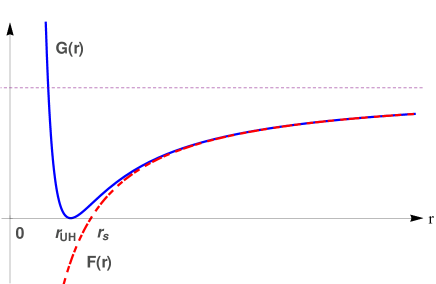
Figure 2: The functions $F(r)$ and $G(r)$ defined in Eq. (IV.1) for the Schwarzschild solution (4.20), where $r=r_{UH}$ is the location of the universal horizon, and $r=r_{s}$ the location of the Killing horizon.

Similarly, for the function $\psi$ Eq.(IV) yields,

$$\psi(r)=-(v-r)+r_{s}\ln\left|1-\frac{r}{r_{s}}\right|+\int{\frac{\sqrt{G}}{FV}dr}$$

$$=\psi_{2}-(v-r)+r_{s}\ln\left|1-\frac{r}{r_{s}}\right|-\frac{\epsilon_{UH}}{108r_{s}^{2}}\Bigg{\{}-\psi_{1}$$

$$~{}~{}+\sqrt{48r^{2}+24r_{s}r+9r_{s}^{2}}\left(16r^{2}+8r_{s}r+15r_{s}^{2}\right)$$

$$~{}~{}+60\sqrt{3}r_{s}^{3}\ln\left(4r+r_{s}+\sqrt{16r^{2}+8r_{s}r+3r_{s}^{2}}\right)$$

$$~{}~{}+108r_{s}^{3}\ln\left[\frac{\left|r-r_{s}\right|}{20r+7r_{s}+3\sqrt{48r^{2}+24r_{s}r+9r_{s}^{2}}}\right]\Bigg{\}},$$

where

$$\psi_{1} = 90\sqrt{6}r_{s}^{3}-108r_{s}^{3}\ln\left(88+36\sqrt{6}\right)$$ (4.29)

$$+60\sqrt{3}r_{s}^{3}\ln\left[\left(4+3\sqrt{2}\right)r_{s}\right],$$

and $\psi_{2}$ is an integration constant. Requiring that $\psi(r)|_{r\rightarrow 0}\rightarrow-v$, we obtain

$$\psi_{2} = -\frac{5}{12}+\frac{5}{\sqrt{6}}+\frac{5\ln\left(4+3\sqrt{2}\right)}{3\sqrt{3}}-\frac{5\ln\left(1+\sqrt{3}\right)}{3\sqrt{3}}$$ (4.30)

$$+\ln\left(18\sqrt{6}-44\right).$$

The hypersurfaces of $\phi=$ Constant and $\psi=$ Constant are illustrated, respectively, in Figs.3 and 4, from which one can see that the peeling-off behavior appears indeed only at the universal horizon $r=r_{UH}$ for the khronon field $\phi$, while the lines of $\psi=$ Constant smoothly cross both of the Killing and universal horizons.

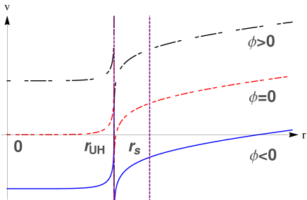
Figure 3: The surfaces of $\phi(v,r)=\phi_{0}$ in the (v, r)-plane for the Schwarzschild solution given by Eq.(4.20).

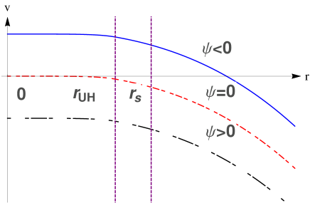
Figure 4: The surfaces of $\psi(v,r)=\psi_{0}$ in the (v, r)-plane with different $\psi_{0}$’s for the Schwarzschild solution given by Eq.(4.20).

In the ($\tau,r$)-planes, the hypersurfaces of $\phi=$ Constant and $\psi=$ Constant are given, respectively, in Figs.5 and 6. Similar to what happened in the ($v,r$)-plane, the peeling-off behavior appears also only at the universal horizon $r=r_{UH}$.

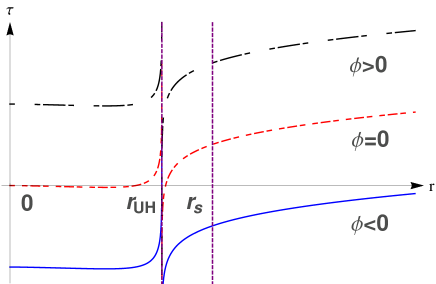
Figure 5: The surfaces of $\phi(\tau,r)=\phi_{0}$ in the ($\tau$, r)-plane for the Schwarzschild solution given by Eq.(4.20).

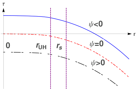
Figure 6: The surfaces of $\psi(\tau,r)=\psi_{0}$ in the ($\tau$, r)-plane with different $\psi_{0}$’s for the Schwarzschild solution given by Eq.(4.20).

The surface gravities on the universal and killing horizons are given by,

$$\kappa_{UH} = \left(\frac{2}{3}\right)^{3/2}\frac{1}{r_{s}},$$

$$\kappa^{GR}_{EH} \equiv \left.\frac{1}{2}F^{\prime}(r)\right|_{r=r_{s}}=\frac{1}{2r_{s}},$$ (4.31)

which are plotted in Fig.7 vs $r_{s}$, where $\kappa^{GR}_{EH}$ denotes the surface gravity at the Killing horizons normally defined in GR. In the current case, $\kappa_{UH}$ is always greater than $\kappa_{EH}$ and $\kappa^{GR}_{EH}$, that is, the universal horizon is always hotter than the Killing horizon, considering the standard relation $\kappa=2\pi T$.

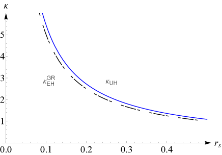
Figure 7: The surface gravities on the killing and universal horizons for the Schwarzschild solution given by Eq.(4.20).

IV.2 Schwarzschild Anti-de Sitter Solution

The Schwarzschild anti-de Sitter solution is given by,

$$F(r)=1-\frac{r_{s}}{r}+\frac{r^{2}}{\ell^{2}},\;\;\;k=1,$$ (4.32)

where $\ell\equiv\sqrt{3/|\Lambda|},\;r_{s}\equiv 2m=\left(1+\frac{r_{EH}^{2}}{\ell^{2}}\right)r_{EH}$, where $r_{EH}$ denotes the Killing horizon of the Schwarzschild anti-de Sitter black hole . Then, from Eq.(4.13) we find that

$$r_{o}^{2} = \frac{1}{18C_{r}^{1/3}\ell}\left[2^{5/3}C_{r}^{4/3}\ell^{4}+64\times 2^{1/3}\ell^{8}\right.$$

$$-27\times 2^{1/3}C_{r}\left(r_{EH}\ell^{4}+r_{EH}^{3}\ell^{2}\right)$$

$$+108\times 2^{2/3}C_{r}^{1/3}\left(r_{EH}\ell^{6}+r_{EH}^{3}\ell^{4}\right)$$

$$+C_{r}^{2/3}\big{(}81\ell^{4}r_{EH}^{2}-32\ell^{6}$$

$$+162\ell^{2}r_{EH}^{4}+81r_{EH}^{6}\big{)}\Big{]}^{2},$$

$$C_{r} = 27r_{EH}\left(r_{EH}^{2}+\ell^{2}\right)$$

$$+\sqrt{128\ell^{6}+729\left(r_{EH}\ell^{2}+r_{EH}^{3}\right)^{1/2}},$$

$$r_{UH} = \frac{2^{1/3}C_{r}^{2/3}-2^{8/3}\ell^{2}}{6C_{r}^{1/3}}.$$ (4.33)

Thus, in terms of $r_{UH}$ and $r_{EH}$, we obtain

$$G(r) = 1-\frac{r_{s}}{r}+\frac{r^{2}}{\ell^{2}}+\frac{r_{o}^{4}}{r^{4}}$$ (4.34)

$$= \frac{(r-r_{UH})^{2}}{\ell^{2}r^{4}}\Big{[}r^{4}+2r_{UH}r^{3}$$

$$+\left(\ell^{2}+3r_{UH}^{2}\right)r^{2}$$

$$-\big{(}4r_{UH}^{3}-r_{EH}^{2}-r_{EH}\ell^{2}$$

$$+2r_{UH}\ell^{2}\big{)}r-2r_{EH}^{3}r_{UH}$$

$$\left.+5r_{UH}^{4}-2r_{EH}r_{UH}\ell^{2}+3r_{UH}^{2}\ell^{2}\right].$$

In Fig.8 we show the curves of $G(r)$ and $F(r)$ vs $r$. Comparing it with that of Fig.2 for the Schwarzschild solution, one can see the similarities between these two cases.

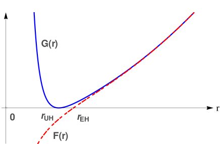
Figure 8: The functions $F(r)$ and $G(r)$ defined in Eq.(IV.2) for the Schwarzschild Anti-de Sitter solution (4.32).

In the current case, it is difficulty to obtain analytic solutions for $\phi$ and $\psi$. Instead, we consider the numerical ones. In particular, in the ($v,r$)-plane the hypersurfaces of $\phi=$ Constant are presented in Figs.9, while the hypersurfaces of $\psi=$ Constant are presented in Figs.10. Again, peeling-off behavior happens only at the universal horizon.

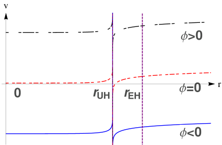
Figure 9: The surfaces of $\phi(v,r)=\phi_{0}$ in the (v, r)-plane for the Schwarzschild Anti-de Sitter solution given by Eqs.(4.32)-(4.34).

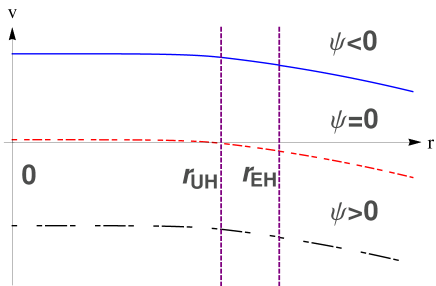
Figure 10: The surfaces of $\psi(v,r)=\psi_{0}$ in the (v, r)-plane for the Schwarzschild Anti-de Sitter solution given by Eqs.(4.32)-(4.34).

Note that the Schwarzschild Anti-de Sitter solution in the Painleve-Gullstrand coordinates ($\tau,r$) is not well-defined for $r\gg\ell$, as now $N^{r}=\sqrt{1-F(r)}$ becomes imaginary when $r$ is sufficiently large.

Finally, the surface gravities on the universal and killing horizons are given by

$$\kappa_{UH} = \frac{\sqrt{3}r_{o}^{2}}{2\ell r_{UH}^{7/2}}\sqrt{5r_{UH}^{3}-r_{EH}^{3}-\ell^{2}(r_{EH}-2r_{UH})},$$

$$\kappa^{GR}_{EH} = \left.\frac{1}{2}F^{\prime}(r)\right|_{r=r_{EH}}=\frac{1}{2}\left(\frac{1}{r_{EH}}+3\frac{r_{EH}}{\ell^{2}}\right),$$ (4.35)

which are shown in Fig.11. It is interesting to note that $\kappa_{UH}$ is larger than $\kappa^{GR}_{EH}$ only when $r_{EH}$ is small. There exists a critical value $r_{c}$ at which $\kappa_{UH}=\kappa^{GR}_{EH}$. When $r_{EH}>r_{c}$, we have $\kappa_{UH}<\kappa^{GR}_{EH}$. It should be also noted that in Fig.11 we plot the curves only for $\ell=1$. However, for other values of $\ell$, similar properties are found, as it can be seen from Figs.12 and 13.

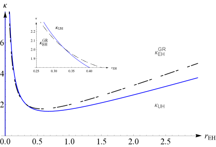
Figure 11: The surface gravities on the killing and universal horizons for the Schwarzschild Anti-de Sitter solution given by Eqs.(4.32)-(4.34). When drawing these curves, we set $\ell=1$.

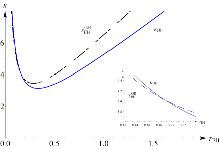
Figure 12: The surface gravities on the killing and universal horizons for the Schwarzschild Anti-de Sitter solution given by Eqs.(4.32)-(4.34). When drawing these curves, we set $\ell=1/2$.

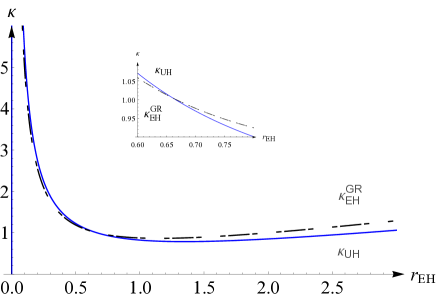
Figure 13: The surface gravities on the killing and universal horizons for the Schwarzschild Anti-de Sitter solution given by Eqs.(4.32)-(4.34). When drawing these curves, we set $\ell=2$.

IV.3 Reissner-Nordström Solution

The Reissner-Nordström (RN) solution is given by,

$$F(r)=1-\frac{r_{s}}{r}+\frac{Q^{2}}{r^{2}},\;\;\;k=1,$$ (4.36)

where $r_{s}\equiv 2m=r_{EH}+r_{IH},\;Q^{2}=r_{EH}r_{IH}$, where $r_{EH}$ and $r_{IH}$ denote the event and inner horizons of the RN solution, respectively. Setting $r_{IH}=br_{EH}$, where $0<b\leq 1$, from Eq.(4.13) we find that

$$r_{o}^{2} = \frac{r_{EH}^{2}}{16\sqrt{2}}\left[27-36b+2b^{2}-36b^{3}+27b^{4}\right.$$

$$\left.+\left(9-5b-5b^{2}+9b^{3}\right)C_{b}\right]^{1/2},$$

$$r_{UH} = \left(3+3b+C_{b}\right)\frac{r_{EH}}{8},$$

$$C_{b} = \sqrt{9-14b+9b^{2}}.$$ (4.37)

Thus, in terms of $r_{UH}$, $r_{IH}$ and $r_{EH}$, we obtain

$$G(r) = 1-\frac{r_{s}}{r}+\frac{Q^{2}}{r^{2}}+\frac{r_{o}^{4}}{r^{4}}$$ (4.38)

$$= \frac{(r-r_{UH})^{2}}{r^{4}}\left(r^{2}+A_{1}r+A_{0}\right),$$

where

$$A_{1} = 2r_{UH}-(1+b)r_{EH},$$

$$A_{0} = br_{EH}^{2}-2br_{UH}-2r_{UH}r_{EH}+3r_{UH}^{2}.~{}~{}~{}~{}$$ (4.39)

In Fig.14 we show the curves of $G(r)$ and $F(r)$ vs $r$ in the non-extreme ($0<b<1$) and extreme ($b=1$) cases, respectively.

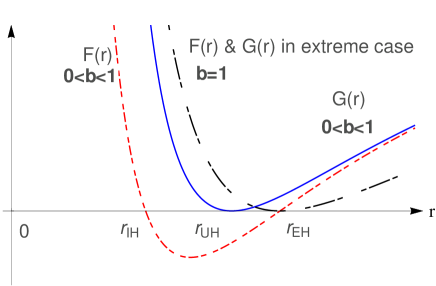
Figure 14: The functions $F(r)$ and $G(r)$ defined in Eqs.(4.36) and (IV.3) for the Reissner-Nordström solution. The solid curve represents the function $G(r)$ for the non-extreme case $0<b<1$, while the dashed curve represents the function $F(r)$ for the non-extreme case. The dot-dashed curve represents the function $G(r)$ for the extreme case $b=1$, for which $F(r)=G(r)$.

In the extreme case $b=1$, the inner, event and universal horizons all coincide. This is because the position of universal horizon is always between the inner and event horizons, in which the killing vector $\zeta^{\mu}$ is space-like. Then, from Eq.(IV.3) we find that $\left.r_{o}^{2}\right|_{b=1}=0$, so that $V=0$ and $G(r)=F(r)$. Hence, from Eq.(IV) we can see that $\psi$ is not well-defined. Redefining $\psi$ as $d\psi=\frac{dr}{\sqrt{F}}$, the metric takes the form,

$$ds^{2}=-\frac{(r-r_{UH})^{2}}{r^{2}}d\phi^{2}+d\psi^{2}+r^{2}d\Omega^{2}_{+1},\;(b=1).$$ (4.40)

In the non-extreme case $0<b<1$, we obtain

$$\phi = v-r-\frac{r_{EH}^{2}}{r_{EH}-r_{IH}}\ln\left|1-\frac{r}{r_{EH}}\right|$$ (4.41)

$$+\frac{r_{IH}^{2}}{r_{EH}-r_{IH}}\ln\left|1-\frac{r}{r_{IH}}\right|-\bar{\varphi}(r)+\bar{\varphi}(0),~{}~{}~{}~{}~{}$$

where

$$\bar{\varphi}(r)=\epsilon_{UH}r_{o}^{2}\left[A_{C}(r_{EH})A_{C}(r_{IH})A_{C}(r_{UH})\right.$$

$$\left.(r_{EH}-r_{IH})(r_{EH}-r_{UH})(r_{IH}-r_{UH})\right]^{-1}$$

$$\times\left[r_{EH}^{2}A_{C}(r_{IH})A_{C}(r_{UH})(r_{IH}-r_{UH})\right.$$

$$\ln\left|\frac{2A_{0}+A_{1}r+A_{1}r_{EH}+2rr_{EH}}{r-r_{EH}}\right.$$

$$\left.+\frac{2A_{C}(r_{EH})A_{C}(r)}{r-r_{EH}}\right|+A_{C}(r_{EH})A_{C}(r_{UH})r_{IH}^{2}$$

$$\times(r_{UH}-r_{EH})\ln\left|\frac{2A_{0}+A_{1}r+A_{1}r_{IH}+2rr_{IH}}{r-r_{IH}}\right.$$

$$\left.+\frac{2A_{C}(r_{IH})A_{C}(r)}{r-r_{IH}}\right|+A_{C}(r_{EH})A_{C}(r_{UI})r_{IU}^{2}$$

$$\times(r_{EH}-r_{IH})\ln\left|\frac{2A_{0}+A_{1}r+A_{1}r_{UH}+2rr_{UH}}{r-r_{UH}}\right.$$

$$\left.\left.+\frac{2A_{C}(r_{UH})A_{C}(r)}{r-r_{UH}}\right|\right],$$

$$A_{C}(r)=\sqrt{A_{0}+A_{1}r+r^{2}}.$$ (4.42)

On the other hand, we have

$$\psi = r-v+\frac{r_{EH}^{2}}{r_{EH}-r_{IH}}\ln\left|1-\frac{r}{r_{EH}}\right|$$ (4.43)

$$-\frac{r_{IH}^{2}}{r_{EH}-r_{IH}}\ln\left|1-\frac{r}{r_{IH}}\right|+\bar{\psi}(r)-\bar{\psi}(0),~{}~{}~{}$$

where

$$\bar{\psi}(r)=\frac{A_{C}(r)}{r_{EH}^{4}}\left[27-36b+2b^{2}-36b^{3}+27b^{4}\right.$$

$$\left.+C_{b}\left(9-5b-5b^{2}+9b^{3}\right)\right]^{-1}\left(\Psi(r)-\Psi(0)\right).$$

$$\Psi(r)=\frac{16}{3}A_{0}-2A_{1}^{2}+\frac{4}{3}A_{1}r+4A_{1}\left(r_{EH}+r_{IH}\right.$$

$$\left.-r_{UH}\right)+\frac{8}{3}\left[2r^{2}+3r\left(r_{EH}+r_{IH}-r_{UH}\right)\right.$$

$$\left.+6\left(r_{EH}^{2}+r_{EH}r_{IH}+r_{IH}^{2}-r_{EH}r_{UH}-r_{IH}r_{UH}\right)\right]$$

$$-A_{C}(r)^{-1}\left\{4A_{0}A_{1}+2\left(A_{1}^{2}-4A_{0}\right)\left(r_{EH}+r_{IH}\right.\right.$$

$$\left.-r_{UH}\right)-A_{1}^{3}-8A_{1}\left[r_{EH}^{2}+\left(r_{IH}+r_{EH}\right)\left(r_{IH}\right.\right.$$

$$\left.\left.-r_{UH}\right)\right]-16\left[r_{EH}^{3}+\left(r_{IH}^{2}+r_{IH}r_{EH}+r_{EH}^{2}\right)\left(r_{IH}\right.\right.$$

$$\left.\left.-r_{UH}\right)\right]\ln\left|2r+A_{1}+2A_{C}(r)\right|$$

$$+16\frac{r_{EH}^{2}A_{C}(r_{EH})\left(r_{EH}-r_{UH}\right)}{A_{C}(r_{r})\left(r_{IH}-r_{EH}\right)}\ln\left|\frac{A_{r}(r_{EH})}{r-r_{EH}}\right|$$

$$\left.+16\frac{r_{IH}^{2}A_{C}(r_{IH})\left(r_{IH}-r_{UH}\right)}{A_{C}(r_{r})\left(r_{EH}-r_{IH}\right)}\ln\left|\frac{A_{r}(r_{IH})}{r-r_{IH}}\right|\right\},$$

$$A_{r}(r_{H})=2A_{0}+A_{1}r+A_{1}r_{H}+2rr_{H}$$

$$+2A_{C}(r_{H})A_{C}(r).$$ (4.44)

In the ($v,r$)-plane, the hypersurfaces of $\phi=$ Constant are given in Figs.15, while the hypersurfaces of $\psi=$ Constant are given in Figs.16, which again are peeling off only at the universal horizon.

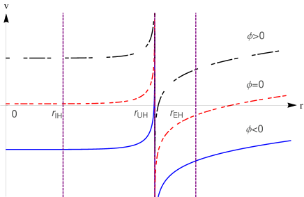
Figure 15: The surfaces of $\phi(v,r)=\phi_{0}$ in the (v, r)-plane for the Reissner-Nordström solution In the non-extreme case $0<b<1$.

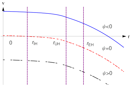
Figure 16: The surfaces of $\psi(v,r)=\psi_{0}$ in the (v, r)-plane for the Reissner-Nordström solution In the non-extreme case $0<b<1$.

Similar to the Schwarzschild Anti-de Sitter solution, the RN solution is also not well-defined in the Painleve-Gullstrand coordinates ($\tau,r$), as now $N^{r}=\sqrt{1-F(r)}$ will become imaginary when $r$ is sufficiently small.

Finally, the surface gravities on the universal and killing horizons are given by

$$\kappa_{UH} = \frac{32\sqrt{2}}{\left(3+3b+C_{b}\right)^{5}r_{EH}}\left\{\left[27-36+2b^{2}-36b^{3}\right.\right.$$

$$\left.+27b^{4}+C_{b}\left(9-5b-5b^{2}+9b^{3}\right)\right]$$

$$\times\left[81-36+22b^{2}-36b^{3}+81b^{4}\right.$$

$$\left.\left.+C_{b}\left(27-9b-9b^{2}+27b^{3}\right)\right]\right\}^{1/2},$$

$$\kappa^{GR}_{EH} = \frac{1-b}{2r_{EH}}.$$ (4.45)

The curves of $\kappa_{UH}$ and $\kappa_{EH}^{GR}$ vs $r_{EU}$ are given in Fig.17. It is interesting to note that, similar to the Schwarzschild anti-de Sitter space-time, in the current case $\kappa_{UH}$ is larger than $\kappa^{GR}_{EH}$ only when $r_{EH}$ is small. There exists a critical value $r_{c}$ at which $\kappa_{UH}=\kappa^{GR}_{EH}$. When $r_{EH}>r_{c}$, we have $\kappa_{UH}<\kappa^{GR}_{EH}$.

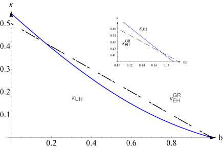
Figure 17: The surface gravities on the killing and universal horizons for the Reissner-Nordström solution In the non-extreme case $0<b<1$. When drawing these curves, we had set $r_{EH}=1$.

V Conclusions

In this paper, we have studied the existence of universal horizons in static spacetimes, and found that the khronon field can be solved explicitly when its velocity becomes infinitely large, at which point the universal horizons coincide with the sound horizon of the khronon. Choosing the timelike coordinate aligned with the khronon, the static metric takes the simple form (3.16), which shows clearly that the metric now is free of coordinate singularity at the Killing horizons, but becomes singular at the universal horizons. These singularities are coordinate ones, and can be removed by properly coordinate transformations. For example, in the ($\phi,\psi$)-coordinates (3.16), the metric is well-defined across the Killing horizons $F=0$, while in the Eddington-Finkelstein coordinates (3.1), it is well-defined across the universal horizons $F\alpha^{2}+1=0$.

Applying such definitions to the three well-known black hole solutions, the Schwarzschild, Schwarzschild anti-de Sitter, and Reissner-Nordström, which are often also solutions of gravitational theories with broken LI in the HL gravity GLLSW ; GPW and Einstein-aether theory in the case where the effects of the khronon field is negligible EA , we have shown that in all these solutions universal horizons always exist inside the Killing horizons. The peeling-off behavior of the khronon appears only at the universal horizons.

We have also considered the surface gravity $\kappa_{UH}$ defined in CLMV , which yields the standard relation $T=\kappa/2\pi$ between the Hawking temperature $T$ and the surface gravity $\kappa$ for the particular solutions studied in BBM . In addition, we have shown explicitly that it is equal to $\kappa_{peeling}$ obtained by the peeling behavior of the khronon at the universal horizon [cf. Eqs.(4.16) and (4.19)]. We have also compared the temperature $T_{UH}[\equiv\kappa_{UH}/2\pi]$ with the temperature $T_{EH}^{GR}[\equiv\kappa_{EU}^{GR}/2\pi]$ of the Killing horizon defined in general relativity, and found that $T_{UH}$ is always greater than $T_{EH}^{GR}$ in the Schwarzschild space-time. But in the Schwarzschild anti-de Sitter and Reissner-Nordström spacetimes, there always exists a critical value of $r_{c}$, and when $r_{EU}<r_{c}$, $T_{UH}$ is always larger than $T_{EH}^{GR}$. But, when $r_{EU}>r_{c}$, $T_{UH}$ is always smaller than $T_{EH}^{GR}$.

Appendix A: The Khronon Mode

In the Minkowiski background,

$$ds^{2}=-dt^{2}+dx^{i}dx^{i},\;(i=1,2,3),$$ (A.1)

the khronon equation (2.5) has the solution $\phi=t$. Considering the perturbations of the khronon in this background,

$$\phi=t+\chi(t,x^{i}),$$ (A.2)

where $\chi$ denotes the perturbations, we find that to the second-order, the khronon action takes the form,

$$S_{\phi}^{(2)}=\int dtd^{D}x\left[c_{123}\left(\nabla^{2}\chi\right)^{2}-c_{14}\left(\nabla_{i}\dot{\chi}\right)^{2}\right],$$ (A.3)

where $\dot{\chi}=\partial_{t}\chi$. Then, $\chi$ satisfies the equation,

$$\nabla^{2}\left(\ddot{\chi}-c_{\phi}^{2}\nabla^{2}\chi\right)=0,$$ (A.4)

where $c_{\phi}$ is defined by Eq.(2.9). The above equation shows that there are two different modes, one is propagating with a speed $c_{\phi}$, and the other is propagating with an infinitely large speed (instantaneous propagation) BS11 . It should be also noted the difference between the speed of the Khronon and the speed of the spin-0 mode of the aether JM04 ,

$$c_{\phi,JM}^{2}=\frac{c_{123}(2-c_{14})}{c_{14}(1-c_{13})(2+c_{13}+3c_{2})}.$$ (A.5)

When $|c_{i}|\ll 1$, it reduces to the one given by Eq.(2.9).