Analyzing the Fault-Containment Time of Self-Stabilizing Algorithms — A Case Study for Graph Coloring

Abstract

The paper presents techniques to derive upper bounds for the mean time to recover from a single fault for self-stabilizing algorithms in the message passing model. For a new $\Delta+1$-coloring algorithm we analytically derive a bound for the mean time to recover and show that the variance is bounded by a small constant independent of the network’s size. For the class of bounded-independence graphs (e.g. unit disc graphs) all containment metrics are in $O(1)$.

1 Introduction

Fault tolerance aims at making distributed systems more reliable by enabling them to continue the provision of services in the presence of faults. The strongest form is masking fault tolerance, where a system continues to operate after faults without any observable impairment of functionality, i.e. safety is always guaranteed. In contrast non-masking fault tolerance does not ensure safety at all times. Users may experience a certain amount of incorrect system behavior, but eventually the system will fully recover. The potential of this concept lies in the fact that it can be used in cases where masking fault tolerance is too costly or even impossible to implement [11]. Systems that eventually recover from transient faults of any scale such as perturbations of the state in memory or communication message corruption are called self-stabilizing. A critical issue is the length of the time span until full recovery. Examples are known where a memory corruption at a single process caused a vast disruption in large parts of the system and triggered a cascade of corrections to reestablish safety. Thus, an important issue is the reduction of the effect of transient faults in terms of time and space until a safe state is reached.

A fault-containing system has the ability to contain the effects of transient faults in space and time. The goal is keep the extend of disruption during recovery proportional to the extent of the faults. An extreme case of fault-containment with respect to space is given when the effect of faults is bounded exactly to the set of faulty nodes. Azar et al. call this form error confinement [1]. More relaxed forms of fault-containment are known as time-adaptive self-stabilization [18], scalable self-stabilization [13], strict stabilization [21], strong stabilization [8], and 1-adaptive self-stabilization [3].

A large body of research focuses on fault-containing in the $1$-faulty case. A configuration is called $k$-faulty, if in a legitimate configuration exactly $k$ processes are hit by a fault. Several metrics have been introduced to quantify the containment behavior in the $1$-faulty case [12, 17]. A distributed algorithm ${\cal A}$ has contamination radius $r$ if only nodes within the $r$-hop neighborhood of the faulty node change their state during recovery from a 1-faulty configuration. The containment time of ${\cal A}$ denotes the worst-case number of rounds any execution of ${\cal A}$ starting at a 1-faulty configuration needs to reach a legitimate configuration. In technical terms this corresponds to the worst case time to recover in case of a single fault. For randomized algorithms the expected number of rounds to reach a legitimate configuration corresponds to the mean time to recover (MTT).

The stabilization time is an obvious upper bound for the containment time. In some cases this bound can be improved, for example when the contamination radius is known. In the shared memory model an algorithm with contamination radius $r$ and stabilization time $O(f(n))$ obviously has containment time $O(f(\Delta^{r}))$. There are only few cases where the containment time is explicitly computed and in these cases only asymptotic bounds are given. From a practical point of view absolute bounds are more valuable.

The focus of this paper is on the analysis of the containment time of randomized self-stabilizing algorithms in the message passing model with respect to memory and message corruption. We show how Markov chains can be used to find upper bounds for the containment time that are lower than the above mentioned trivial bound $O(f(\Delta^{r}))$. For a $\Delta+1$-coloring algorithm we analytically derive an absolute bound for the expected containment time and show that the variance is surprisingly bounded by a small constant independent of the network’s size. We believe that the presented techniques can also be applied to other algorithms.

2 Related Work

There exist several techniques to analyze self-stabilizing algorithms: potential functions, convergence stairs, Markov chains, etc. Markov chains are particular useful for randomized algorithms [9]. Their main drawback is that in order to set up the transition matrix the adjacency matrix of the graph must be known. This restricts the applicability of this method to small or highly symmetric instances. DeVille and Mitra apply model checking tools to Markov chains for cases of networks of small size ($n\leq 7$) to determine the expected stabilization time [5]. An example for highly symmetric networks are ring topologies, see for example [10, 23]. Fribourg et al. model randomized distributed algorithms as Markov chains using the technique of coupling to compute upper bounds for the stabilization times [10]. Yamashita uses Markov chains to model self-stabilizing probabilistic algorithms and to prove stabilization [23]. Mitton et al. consider a randomized self-stabilizing $\Delta+1$-coloring algorithm and model this algorithm in terms of urns/balls using a Markov chain to get a bound for the stabilization time [20]. They evaluated the Markov chain for networks up to 1000 nodes analytically and by simulations. Crouzen et al. model faulty distributed algorithms as Markov decision processes to incorporate the effects of random faults when using a non-deterministic scheduler [4]. They used the PRISM model-checker to compute long-run average availabilities. The above literature considered only the shared memory model.

3 Bounding the Containment Time

The containment time is a special case of the stabilization time. The difference is that only executions starting from $1$-faulty configurations are considered. Such configurations arise when a single node $v$ is hit by a memory corruption or a single message sent by $v$ is corrupted. We do not consider corruptions of the code of an algorithm. Denote by $R_{v}$ the subgraph of the communication graph $G$ that is induced by the nodes that are engaged in the recovery process from a $1$-faulty configuration triggered by a fault at $v$. There are two situations in which it is apparently feasible to obtain bounds for the containment time that are lower than the above mentioned trivial bound of $O(f(|R_{v}|)$: Either the structure of $R_{v}$ is considerably simpler than that of $G$ or $R_{v}$’s size is smaller than that of $G$.

3.1 Shared Memory Model

First consider the shared memory model. If an algorithm has contamination radius $r$ and no other fault occurs then this fault will not spread beyond the $r$-hop neighborhood of the faulty node $v$. In this case $R_{v}\subseteq G_{v}^{r}$, where $G_{v}^{r}$ is the subgraph induced by $v$ and nodes $w$ with $dist(v,w)\leq r$. The analysis of the containment time is often simplified due to the fact that the initial configuration is almost legitimate (i.e., only $v$ is not legitimate).

As a first example consider the well known self-stabilizing Algorithm $\mathcal{A}_{1}$ to compute a maximal independent set (MIS).

if $state=IN\wedge\exists w\in N(v)$ s.t. $w.state=IN$ then

      $state:=OUT$

if $state=OUT\wedge\forall w\in N(v)$ $w.state=OUT$ then

       if random bit from 0,1 = 1 then

            $state:=IN$

      

Algorithm 1 Self-stabilizing algorithm $\mathcal{A}_{1}$ to compute a MIS.

Lemma 3.1

Algorithm $\mathcal{A}_{1}$ has contamination radius two.

• Let $v$ be a node hit by a memory corruption. First suppose the state of $v$ changes from $IN$ to $OUT$. Let $u\in N(v)$ then $u.state=OUT$. If $u$ has an neighbor $w\not=v$ with $w.state=IN$ then $u$ will not change its state during recovery. Otherwise, if all neighbors of $u$ except $v$ had state $OUT$ node $u$ may change state during recovery. But since these neighbors of $u$ have a neighbor with state $IN$ they will not change their state. Thus, in this case only the neighbors of $v$ may change state during recovery.

  Next suppose that $v.state$ changes from $OUT$ to $IN$. Then $v$ and those neighbors of $v$ with state $IN$ can change to $OUT$. Then arguing as in the first case only nodes within distance two of $v$ may change their state during recovery.

Graph $R_{v}$ can contain any subgraph $H$ with $\Delta(G)$ nodes. For example let $G$ consist of $H$ and an additional vertex $v$ connected to each node of $H$. A legitimate configuration is given if the state of $v$ is $IN$ and all other nodes have state $OUT$ (Fig. 1 left). If $v$ changes its state to $OUT$ due to a fault then all nodes may change to state $IN$ during the next round. A precise analysis of the containment time depends extremely on the structure of $H$. Thus, there is little hope for a bound below the trivial bound. Similar arguments hold for the second 1-faulty configuration of $\mathcal{A}_{1}$ shown on the right of Fig. 1.

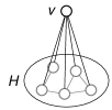
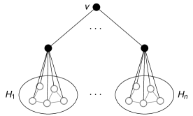
Figure 1: 1-faulty configurations of $\mathcal{A}_{1}$ caused by a memory corruption at $v$. Nodes drawn in bold have state $IN$. The depicted graphs correspond to $R_{v}$.

Next we consider the problem of finding a $\Delta+1$-coloring. Almost all self-stabilizing algorithms for this problem follow the same pattern. A node that realizes that it has chosen the same color as one of its neighbors chooses a new color from a finite color palette. This palette does not include the current colors of the node’s neighbors. To be executed under the synchronous scheduler these algorithms are either randomized or use identifiers for symmetry breaking. Variations of this idea are followed in [7, 14, 21, 20]. As an example consider Algorithm $\mathcal{A}_{2}$ from [14]. Due to its choice of a new color from the palette $\mathcal{A}_{2}$ has contamination radius at least $\Delta(G)$ (see Fig. 2).

if $c\not=\max\left(\{0,\ldots,\Delta\}\backslash\{w.c\mid w\in N(v)\}\right)$ then

       if random bit from 0,1 = 1 then

            $c:=\max\left(\{0,\ldots,\Delta\}\backslash\{w.c\mid w\in N(v)\}\right)$

      

Algorithm 2 Self-stabilizing $\Delta+1$-coloring algorithm $\mathcal{A}_{2}$ from [14].

Figure 2: Algorithm $\mathcal{A}_{2}$ has contamination radius $\Delta$: If the left-most node is hit by a fault and changes its color to $\Delta-1$, then all other nodes may change their color.

For some problems minor modifications of the algorithms can lead to dramatic changes of the contamination radius. Algorithm $\mathcal{A}_{3}$ is a slight modification of this algorithm. $\mathcal{A}_{3}$ has containment radius $1$ (see Lemma 3.2) and $R_{v}$ is a star graph with center $v$. Note that neighbors of $v$ that change their color during recovery form an independent set. This simple structure allows an analysis of the containment time.

if $\exists w\in N(v)$ s.t. $c=w.c$ then

       if random bit from 0,1 = 1 then

            $c:=$ choose $\{0,\ldots,\Delta\}\backslash\{w.c\mid w\in N(v)\}$

      

Algorithm 3 Self-stabilizing $\Delta+1$-coloring algorithm $\mathcal{A}_{3}$.

Lemma 3.2

Algorithm $\mathcal{A}_{3}$ has contamination radius one.

• Let $v$ be a node hit by a memory corruption changing its color to a color $c$ already chosen by at least one neighbor of $v$. Let $N_{conf}=\{w\in N(v)\mid w.c=c\}$. In the next round the nodes in $N_{conf}\cup\{v\}$ will get a chance to choose a new color. The choices will only lead to conflicts between $v$ and others nodes in $N_{conf}$. Thus, the fault will not spread beyond the set $N_{conf}$. With a positive probability the set $N_{conf}$ will contain fewer nodes in each round.

3.2 Message Passing Model

In the message passing model the situation is different for two reasons. First of all, a $1$-faulty configuration is also given when a single message sent by a node $v$ is corrupted. Secondly, this may cause neighbors of $v$ to send messages they would not send in a legitimate configuration. Even so the state of nodes with distance greater than $r$ to $v$ does not change, these nodes may be forced to send messages. Thus, in general the analysis of the containment time cannot be performed by considering $G_{v}^{r}$ only. This is only possible in cases when a fault at $v$ does not force nodes at distance $r+1$ to send messages they would not send had the fault not occurred.

4 Computing the Expected Containment Time

A randomized synchronous self-stabilizing algorithm ${\cal A}$ can be regarded as a transition systems. Denote by $\Sigma$ the set of all configurations. In each round the current configuration $c\in\Sigma$ is transformed into a new configuration ${\cal A}(c)\in\Sigma$. This process is described by the transition matrix $P$ where $p_{ij}$ gives the probability to move from configuration $c_{i}$ to $c_{j}$ in one round, i.e., ${\cal A}(c_{i})=c_{j}$.

To compute the containment time one must consider all executions starting from a $1$-faulty configuration $c$. Let $X$ be the random variable that denotes the number of rounds until the system has reached a legitimate configuration when starting in $c$. The expected containment time equals the expected value $E[X]$. In some cases it is possible to compute $E[X]$ directly according to the definition. But in most cases this will be impossible.

To reduce the complexity it is often helpful to partition $\Sigma$ into subsets $S_{0},\ldots,S_{l}$ and consider these as the states of a Markov chain. The subsets must have the property that for each pair of subsets $S_{i},S_{j}$ the probability of a configuration $c\in S_{i}$ to be transformed in one round into a configuration of $S_{j}$ is independent of the choice of $c\in S_{i}$. This probability is then interpreted as the transition probability from $S_{i}$ to $S_{j}$. This way the complexity of the analysis can often be reduced dramatically.

A state $c_{i}$ of a Markov chain is called absorbing if $p_{ii}=1$ and $p_{ij}=0$ for $i\not=j$. For self-stabilizing algorithms, the set of all legitimate configurations $\cal L$ is an absorbing state, in fact it is the unique absorbing state in this case. The number of rounds to reach a legitimate configuration starting from a given configuration $c_{i}\in S_{i}$ equals the number of steps before being absorbed in $\cal L$ when starting in state $S_{i}$. This equivalence allows to use techniques from Markow chains to compute the stabilization time and thus, the containment time.

To compute the containment time we must consider all executions starting from a fixed $1$-faulty configuration. Let $S_{0}$ consist of a single $1$-faulty configuration and $S_{l}$ be the set of all legitimate configurations. It suffices to compute the expected number of rounds to reach $S_{l}$ from $S_{0}$ and then take the maximum for all $1$-faulty configurations.

4.0.1 Example

As an example consider algorithm $\mathcal{A}_{3}$ as described above. Let $c$ be a legitimate configuration and $v$ be a node that changes its color due to a memory fault. This causes a conflict with all $d$ neighbors of $v$ that had chosen this color. During the execution of $\mathcal{A}_{3}$ only nodes contained in $R_{v}$ (a star graph) change their state. Furthermore, once a neighbor has chosen a color different from $v$ then the choice will be forever (at least until the next transient fault).

Let $d$ be the number of neighbors of $v$ that have the same color as $v$ after the fault. Denote by $S_{j}$ the set of all configurations reachable from $c$ where exactly $d-j$ neighbors of $v$ have the same color as $v$. Then $S_{0}=\{c\}$ and $S_{d}$ consists of all legitimate configurations. Let $c_{i}\in S_{i}$. Then $\mathcal{A}_{3}(c_{i})\not\in S_{j}$ for all $j<i$. Unfortunately, the probability of a configuration $c_{i}\in S_{i}$ to be transformed in one round into a configuration of $S_{j}$ for $j>i$ is not independent of the choice of $c_{i}\in S_{i}$. But it is possible to resolve this issue as shown below.

4.1 Absorbing Markov Chains

Let $S_{0},\ldots,S_{d}$ be nonempty subsets of $\Sigma$ and $P$ a stochastic matrix such that $P({\cal A}(c)\in S_{j})=p_{ij}$ for all $i,j\in\{0,1,\ldots,d\}$ and all $c\in S_{i}$. Furthermore, let $S_{d}$ be the single absorbing state. Let $Q$ be the matrix obtained from $P$ by removing the last row and the last column. $Q$ describes the probability of transitioning from some transient state to another. The following properties about absorbing Markov chains are well known and can be found in Theorem 3.3.5 of [16]. Denote the $d\times d$ identity matrix by $E_{d}$. Then

$$N=(E_{d}-Q)^{-1}$$

is the fundamental matrix of the Markov chain. The expected number of steps before being absorbed by $S_{d}$ when starting from $S_{i}$ is the $i$-th entry of vector

$$a=NI_{d}$$

where $I_{d}$ is a length-$d$ column vector whose entries are all 1. The variance of these numbers of steps is given by the entries of

$$(2N-E_{d})a-a_{sq}$$

where $a_{sq}$ is derived from $a$ by squaring each entry.

4.1.1 Example

To apply the results of the last section to algorithm $\mathcal{A}_{3}$ the following adjustments are made. For $i<j$ let $p_{ij}$ be a constant such that $P(\mathcal{A}_{3}(c_{i})\in S_{j})\geq p_{ij}$ for all $c_{i}\in S_{i}$. Furthermore, let $p_{ij}=0$ for $j<i$ and

$$p_{ii}=1-\sum_{k=j+1}^{d}p_{ij}$$

for $i=0,\ldots,d$. Then matrix $(p_{ij})$ is a stochastic matrix with $p_{dd}=1$. Furthermore, the expected number of steps before being absorbed by state $d$ when starting from state $i$ is an upper bound for the expected number of rounds before being absorbed by state $S_{d}$ when starting from state $S_{i}$. Thus, the results from the last section can be used to find an upper bound for the expected containment time of algorithm $\mathcal{A}_{3}$.

These techniques are applied to the self-stabilizing coloring algorithm $\mathcal{A}_{col}$.

5 Algorithm $\mathcal{A}_{col}$

Computing a $\Delta+1$-coloring in expected $O(\log n)$ rounds with a randomized algorithm is long known [19, 15]. The $(\Delta+1)$-coloring algorithm $\mathcal{A}_{col}$ analyzed in this work follows the pattern sketched in section 3.1. It is derived from a non-self-stabilizing algorithm contained in [2] (Algorithm 19). The presented techniques can also be applied to other randomized coloring algorithms such as those described in [7, 14, 21, 20]. The main difference is that $\mathcal{A}_{col}$ assumes the message passing model, more precisely the synchronous ${\cal CONGEST}$ model as defined in [22]. $\mathcal{A}_{col}$ stabilizes after $O(\log n)$ rounds with high probability whereas the above cited algorithms require a linear number of rounds.

At the beginning of each round of $\mathcal{A}_{col}$ each node broadcasts its current color to its neighbors. Based on the information received from its neighbors a node decides either to keep its color (final choice), to choose a new color or no color (value $\bot$). In particular with equal probability a node $v$ draws uniformly at random a color from the set $\{0,1,\dots,\delta(v)\}\backslash tabu$ or indicates that it made no choice (see Function randomColor). Here, $tabu$ is the set of colors of neighbors of $v$ that already made their final choice.

Color randomColor(Node v, Set<Color> tabu)

       if random bit from 0,1 = 1 then  return $\bot$ ;

       return random color from $\{$0,1,$\ldots,\delta(v)\}\backslash$tabu;

      

In the algorithm of [2] a node maintains a list with the colors of those neighbors that made their final choice. A fault changing the content of this list is difficult to contain. Furthermore, in order to notice a memory corruption at a neighbor, each node must continuously send its state to all its neighbors and cannot stop to do so. This is the price of self-stabilization and well known [6]. These considerations lead to the design of Algorithm $\mathcal{A}_{col}$. Each node only maintains the chosen color (variable c) and whether its choice is final (variable final). In every round a node sends these two variables to all neighbors. To improve fault containment a node’s final choice of a color is only withdrawn if it coincides with the final choice of a neighbor. To achieve a $\Delta+1$-coloring a node makes a new choice if its color is larger than its degree. Note that this situation can only originate from a fault.

Set<Color> tabu := $\emptyset$, occupied := $\emptyset$;

broadcast(c, final) to all neighbors w $\in$ N(v);

for all neighbors w $\in$ N(v) do

       receive(c_w, final_w) from node $w$;

       if $c_{w}\not=\bot$ then

             occupied := occupied $\cup\leavevmode\nobreak\ \{$c${}_{w}\}$;

             if final_w then  tabu := tabu $\cup\leavevmode\nobreak\ \{$c${}_{w}\}$ ;

            

      

if c = $\bot\vee c>\delta(v)$ then

       final := false;

      

else

       if final then

             if $c\in$ tabu then  final := false ;

            

      else

             if $c\not\in$ occupied then  final := true ;

            

      

if final = false then  c := randomColor(v, tabu) ;

Algorithm 4 $\mathcal{A}_{col}$ as executed by a node $v$.

Theorem 5.1 states the correctness and the stabilization time of ${\cal A}_{col}$. The algorithm works correctly for any initial setting of the variables. Note that if $v.final=true$ one round after a transient fault or the initial start $v$ will not change its color until the next fault. With this observation the theorem can be proved along the same lines as Lemma 10.3 in [2].

Theorem 5.1

Algorithm ${\cal A}_{col}$ is self-stabilizing and computes a $\Delta+1$-coloring within $O(\log n)$ time with high probability (i.e. with probability at least $1-n^{c}$ for any $c\geq 1$). ${\cal A}_{col}$ has contamination radius $1$.

First we consider error-free executions, i.e. executions during which no memory nor message corruptions occurs. Note that ${\cal A}_{col}$ must work correctly for any initial setting of the variables. A configuration is called a legal coloring if the values of variable $c$ form a $\Delta+1$-coloring of the graph. It is called legitimate if is a legal coloring and $v.final=true$ for each node $v$. A node $v$ pauses in round $r$ if it does not change the value of $v.c$ or $v.final$ in round $r$. A node $v$ terminates in round $r$ if it pauses in round $r$ and all following rounds.

Lemma 5.2

Let $e$ be an error-free execution and let $v\in V$. If $v$ pauses in round $r$ of $e$ then $v.final=true$ and $v$ terminates in round $r$.

• The only constellation at the beginning of a round in which $v$ pauses is $v.final=true$, $c\in\{0,1,\ldots,\delta(v)\}$, and $c\not\in v.tabu$. The latter condition implies that each neighbor $w$ of $v$ with $w.c=v.c$ at the beginning of round $r$ has sent $w.final=false$ to $v$. Since $v$ sent $(v.c,true)$ to each neighbor, no node $w\in N(v)$ will at the end of round $r$ have $w.c=v.c$ and $w.final=true$. This implies, that in the following round still $v.c\not\in v.tabu$ holds. Thus, $v$ also pauses in round $r+1$. This proves that $v$ terminates in round $r$.

Lemma 5.3

Let $r$ be a round of an error-free execution and let $v\in V$. If $v.final=true$ at the beginning and $v.final=false$ at the end of round $r$ then $r=1$.

• Denote the value of $v.c$ at the beginning of round $r$ by $c_{r}$. In order for $v$ to set $v.final$ to $false$ one of the following three conditions must be met at the beginning of round $r$:

  1. $c_{r}>\delta(v)$,

  2. $c_{r}=\bot$, or

  3. $v$ has a neighbor $w$ with $w.final=true$ and $w.c=c_{r}$.

  The first condition can only be true in round $1$. Suppose that $c_{r}=\bot$ and $v.final=true$ at the beginning of round $r$ with $r>1$. If during round $r-1$ the value of $v.final$ was set to $true$ then $v.c$ could not be $\bot$. Hence, at the beginning of round $r-1$ already $v.final=true$. But then $v.c$ was not changed in round $r-1$, hence $v.c=\bot$ at the beginning of round $r-1$, i.e. $v$ paused in round $r-1$ but did not terminate. This is a contradiction with Lemma 5.2. Finally assume the last condition. Then $v$ and $w$ cannot have changed their value of variable $c$ in round $r-1$, because then variable $final$ could not have value $true$ at the beginning of round $r$. Thus, $v$ sent $(c_{r},true)$ in round $r-1$. Hence, if $w.c=c_{r}$ at that time $w$ would have changed $w.final$ to $false$, contradiction.

Lemma 5.4

A node setting $final$ to $true$ in round $r$ terminates in round $r+1$.

• A node $v$ that sets $v.final$ to $true$ satisfies $v.c\in\{0,1,\ldots,\delta(v)\}$ and all $w\in N(v)$ have $w.c\not=v.c$ at the beginning of round $r$. Also $v$ does not change its color during round $r$. Thus, no $w\in N(v)$ will change its color to $v.c$ during round $r$. Thus, at the beginning or the next round $v.final=true$ and $v.c\not\in v.tabu$. This yields that $v$ pauses in round $r+1$. The result follows from Lemma 5.2.

Lemma 5.5

If all nodes have terminated the configuration is legitimate.

• Let $r$ be a round in which all nodes pause. By Lemma 5.2 all $v\in V$ satisfy $v.final=true$ in this round. Furthermore, since no node changes variable $c$ in round $r$, $v.c\not\in v.tabu$ for each $v\in V$. Thus, $v.c\not=w.c$ for each $w\in N(v)$ and therefore variable $c$ constitutes a valid coloring. Finally, note that because of $v.c\in\{0,1,\ldots,\delta(v)\}$ at most $\Delta+1$ colors are used.

• According to Lemma 5.5 it suffices to prove that all nodes terminate within $O(\log n)$ time with high probability. Let $v\in V$. Lemma 5.4 implies that the probability that $v$ terminates in round $r>1$ is equal to the probability that $v$ sets its variable $v.final$ to $true$ in round $r-1$. This is the probability that $v$ selects a color different from $\bot$ and from the selections of all neighbors that chose a value different from $\bot$ in round $r-2$. Suppose that indeed $v.c\not=\bot$ at the end of round $r-2$. Then $v.c\not\in v.tabu$. The probability that a given neighbor $u$ of $v$ selects the same color $u.c=v.c$ in this round is at most $\frac{1}{2(\delta(v)+1-|v.tabu|)}$. This is because the probability that $u$ selects a color different from $\bot$ is $1/2$, and $v$ has $\delta(v)+1-|v.tabu|$ different colors to select from. Since $r>1$ all nodes in $v.tabu$ have $final=true$ and will never change this value. Thus, at most $\delta(v)-|tabu|$ neighbors select a new color. By the union bound, the probability that $v$ selects the same color as a neighbor is at most

  $$\frac{\delta(v)-|v.tabu|}{2(\delta(v)+1-|v.tabu|)}<\frac{1}{2}.$$

  Thus, if $v$ selects a color $v.c\not=\bot$, it is distinct from the colors of its neighbors with probability at least $1/2$. It holds that $v.c\not=\bot$ with probability $1/2$. Hence, $v$ terminates with probability at least $1/4$.

  The probability that a specific node $v$ doesn’t terminate within $r$ rounds is at most $(3/4)^{r}$ . By the union bound, the probability that there exists a vertex $v\in V$ that does not terminate within $r$ rounds is at most $n(3/4)^{r}$. Hence, ${\cal A}_{col}$ terminates after $r=(c+1)4\log n$ rounds, with probability at least $1-n(3/4)^{r}\geq 1-1/n^{c}$ (note that $\log 4/3>1/4$).

6 Fault Containment of Algorithm ${\cal A}_{col}$

In this section the fault containment behavior of ${\cal A}_{col}$ is analyzed. In particular we consider a legitimate configuration in which a single transient error occurs. Two types of transient errors are considered:

1. Memory corruption at node $v$, i.e., the value of at least one of the two variables of $v$ is corrupted.

2. A broadcast message sent by $v$ is corrupted. Note that the alternative implementation of using $\delta(v)$ unicast messages instead a single broadcast has very good fault containment behavior but is much slower.

The independent degree $\delta_{i}(v)$ of a node $v$ is the size of a maximum independent set of $N(v)$. Let $\Delta_{i}(G)=\max\{\delta_{i}(v)\mid v\in V\}$.

6.1 Message Corruption

First consider the case that a single broadcast message sent by $v$ is corrupted, i.e. the message contains a color $c_{f}$ different from $v.c$ or the value $false$ for variable $final$. Since $w.final=true$ for all $w\in N(v)$ the message $(c_{f},false)$ has no effect on any $w\in N(v)$ regardless of the value of $c_{f}$. Thus, this corrupted message has no effect at all.

Next consider the case that $v$ broadcasts the message $(c_{f},true)$ with $c_{f}\not=v.c$. Let $N_{conf}(v)=\{w\in N(v)\mid w.c=c_{f}\}$. The nodes in $N_{conf}(v)$ form an independent set, because they all have the same color. Thus $|N_{conf}(v)|\leq\delta_{i}(v)$.

Lemma 6.1

The contamination radius after a single corruption of a broadcast message sent by node $v$ is $1$, in particular neither $v$ nor a node outside $N_{conf}(v)$ will change its state. At most $\delta_{i}(v)$ nodes change their state during recovery.

• Let $u\in V\backslash N[v]$. This node continues to send $(u.c,true)$ after the fault. Thus, a neighbor of $u$ that changes its color will not change its color to $u.c$. This yields that no neighbor of $u$ will ever send a message with $u.c$ as the first parameter. This is also true in case $u\in N(v)\backslash N_{conf}(v)$. Hence, no node outside $N_{conf}(v)\cup\{v\}$ will change its state, i.e. the contamination radius is $1$.

  Next consider the node $v$ itself. Let $w\in N_{conf}(v)$. When the faulty message is received by $w$ it sets $w.final$ to false. Before the faulty message was sent no neighbor of $v$ had the same color as $v$. Thus, in the worst case a node $w\in N_{conf}(v)$ will choose $v.c$ as its new color and send $(v.c,false)$ to all neighbors. Since $v.final=true$ this will not force $v$ to change its state. Thus, $v$ keeps broadcasting $(v.c,true)$ and therefore no neighbor $w$ of $v$ will ever reach the state $w.c=v.c$ and $w.final=true$. Hence $v$ will never change its state.

Theorem 5.1 implies that the containment time of this fault is $O(\log\delta_{i}(v))$ with high probability. The following lemma gives a more precise bound.

Lemma 6.2

The expected value for the containment time after a corruption of a message broadcasted by node $v$ is at most $\frac{1}{\ln 2}H_{\delta_{i}(v)}+1/2$ rounds ($H_{i}$ denotes the $i^{th}$ harmonic number) with a variance of at most

$$\frac{1}{\ln^{2}2}\sum_{i=1}^{\delta_{i}(v)}\frac{1}{i^{2}}+\frac{1}{4}\leq\frac{\pi^{2}}{6\ln^{2}2}+\frac{1}{4}\approx 3.6737.$$

• After receiving message $(c_{f},true)$ all nodes $w\in N_{conf}(v)$ set $w.final$ to $false$ and with equal probability $w.c$ to $\bot$ or to a random color $c_{w}\in\{0,1,\ldots,\delta(w)\}\backslash w.tabu$. Note that $|w.tabu|\leq\delta(w)$ because $w.tabu=\{u.c\mid u\in N(w)\backslash v\}\cup\{c_{f}\}$. If $w$ chooses a color different from $\bot$ then this color is different from the colors of all of $w$’s neighbors. Also in this case $w$ will terminate after the following round because then it will set $final$ to $true$. Thus, after one round $w$ has chosen a color that is different from the colors of all neighbors with probability at least $1/2$. Furthermore, this color will not change again. After one additional round $w$ reaches a legitimate state.

  Let the random variable $X_{d}$ with $d=|N_{conf}(v)|$ denote the number of rounds until the system has reached a legal coloring. For $w\in N_{conf}(v)$ let $Y_{w}$ be the random variable denoting the number of rounds until $w$ has a legal coloring. By Lemma 6.1 $X_{d}=\max\{Y_{w}\mid w\in N_{conf}(v)\}$. For $i\geq 1$ let $G(i)=P\{X_{d}\leq i\}=P\{\max\{Y_{w}\mid w\in N_{conf}(v)\}\leq i\}$. Since the random variables $Y_{w}$’s are independent $G(i)=(P\{X\leq i\})^{|N_{conf}(v)|}+1$ where $X$ is a geometric random variable with $p=0.5$. Thus,

  $$G(i)=\left(\sum_{j=1}^{i}p(1-p)^{j-1}\right)^{d}$$

  and $G(0)=0$ with $d=|N_{conf}(v)|$. Then $E[X_{d}]=\sum_{i=1}^{\infty}ig(i)$ with probability function $g(i)=P\{X_{d}=i\}$. Let $q=1-p$. Now for $i\geq 1$

  $$g(i)=G(i)-G(i-1)=(1-q^{i})^{d}-(1-q^{i-1})^{d}=$$

  $$=\sum_{j=0}^{d}\binom{d}{j}(-1)^{j+1}(1-q^{j})q^{j(i-1)}=\sum_{j=1}^{d}\binom{d}{j}\frac{(-1)^{j+1}(1-q^{j})}{q^{j}}(q^{j})^{i}.$$

  This implies

  $$E[X_{d}] =\sum_{j=1}^{d}\binom{d}{j}\frac{(-1)^{j+1}(1-q^{j})}{q^{j}}\sum_{i=1}^{\infty}i(q^{j})^{i}=\sum_{j=1}^{d}\binom{d}{j}\frac{(-1)^{j+1}}{(1-q^{j})}$$

  $$=\sum_{j=1}^{d}\binom{d}{j}(-1)^{j+1}\sum_{l=0}^{\infty}(q^{j})^{l}=\sum_{l=0}^{\infty}\sum_{j=1}^{d}\binom{d}{j}(-1)^{j+1}(q^{l})^{j}$$

  $$=\sum_{l=0}^{\infty}\left(1+\sum_{j=0}^{d}\binom{d}{j}(-1)^{j+1}(q^{l})^{j}\right)=\sum_{l=0}^{\infty}(1-(1-q^{l})^{d})$$

  The result follows from Lemma 6.3. The derivation of the formula for the variance can be found in Lemma 6.4.

Lemma 6.3

For fixed $0<q<1$ and fixed $d\geq 1$

$$\sum_{l=0}^{\infty}(1-(1-q^{l})^{d})\in[-\frac{1}{\ln q}H_{d},-\frac{1}{\ln q}H_{d}+1]\text{ \leavevmode\nobreak\ and\leavevmode\nobreak\ }\sum_{l=0}^{\infty}(1-(1-q^{l})^{d})\approx-\frac{1}{\ln q}H_{d}+\frac{1}{2}.$$

• The function $f(x)=1-(1-q^{x})^{d}$ is for fixed values of $d$ decreasing for $x\geq 0$. Furthermore, $f(0)=1$. Hence,

  $$\sum_{l=0}^{\infty}(1-(1-q^{l})^{d})\geq\int_{0}^{\infty}f(x)dx\geq\sum_{l=0}^{\infty}(1-(1-q^{l})^{d})-1.$$

  Using the substitution $u=1-q^{x}$ the integral becomes

  $$-\frac{1}{\ln q}\int_{0}^{\infty}\frac{1-u^{d}}{1-u}du=-\frac{1}{\ln q}\int_{0}^{1}\sum_{i=0}^{d-1}u^{i}du=-\frac{1}{\ln q}\sum_{i=1}^{d}\frac{1}{i}=-\frac{1}{\ln q}H_{d}.$$

  Approximating $\int_{i}^{i+1}f(x)dx$ with $(f(i)+f(i+1))/2$ yields

  $$\sum_{l=0}^{\infty}(1-(1-q^{l})^{d})\approx\int_{0}^{\infty}f(x)dx+\frac{f(0)}{2}=-\frac{1}{\ln q}H_{d}+\frac{1}{2}$$

Lemma 6.4

For $d>0$ the variance of the containment time is at most

$$Var[X_{d}]=\frac{1}{\ln^{2}2}\sum_{i=1}^{d}\frac{1}{i^{2}}+\frac{1}{4}\leq\frac{\pi^{2}}{6\ln^{2}2}+\frac{1}{4}\approx 3.6737.$$

• $$Var[X_{d}] =E[X_{d}^{2}]-E[X_{d}]^{2}=\sum_{i=1}^{\infty}i^{2}g(i)-E[X_{d}]^{2}$$

  By Lemma 6.5

  $$\sum_{i=1}^{\infty}i^{2}g(i) =\sum_{l=1}^{\infty}(2l+1)(1-(1-q^{l})^{d})=2\sum_{l=1}^{\infty}l(1-(1-q^{l})^{d})+E[X_{d}]$$

  Now Lemma 6.6 yields

  $$Var[X_{d}] \approx\frac{2}{\ln^{2}2}\sum_{i=1}^{d}\frac{H_{i}}{i}+E[X_{d}]-E[X_{d}]^{2}$$

  $$\approx\frac{2}{\ln^{2}2}\sum_{i=1}^{d}\frac{H_{i}}{i}+\frac{H_{d}}{\ln 2}+\frac{1}{2}-\left(\frac{H_{d}}{\ln 2}+\frac{1}{2}\right)^{2}$$ Lemma 6.2

  $$=\frac{1}{\ln^{2}2}\left(2\sum_{i=1}^{d}\frac{H_{i}}{i}-H_{d}^{2}\right)+\frac{1}{4}$$

  $$2\sum_{i=1}^{d}\frac{H_{i}}{i}-H_{d}^{2} =2\sum_{i=1}^{d}\sum_{j=1}^{i}\frac{1}{ij}-(1+\frac{1}{2}+\cdots+\frac{1}{d})^{2}$$

  $$=2\sum_{i=1}^{d}\frac{1}{i^{2}}+2\sum_{i=1}^{d}\sum_{j=1}^{i-1}\frac{1}{ij}-2\sum_{i=1}^{d}\sum_{j=1}^{i-1}\frac{1}{ij}-\sum_{i=1}^{d}\frac{1}{d^{2}}=\sum_{i=1}^{d}\frac{1}{i^{2}}=\frac{\pi^{2}}{6}$$

Lemma 6.5

Let $d>0$, $q\in(0,1)$ and $g(i)=\sum\limits_{j=1}^{d}\binom{d}{j}\frac{(-1)^{j+1}(1-q^{j})}{q^{j}}(q^{j})^{i}$. Then

$$\sum_{i=1}^{\infty}i^{2}g(i)=\sum_{l=1}^{\infty}(2l+1)(1-(1-q^{l})^{d})$$

• $$\sum_{i=1}^{\infty}i^{2}g(i) =\sum_{j=1}^{d}\binom{d}{j}\frac{(-1)^{j+1}(1-q^{j})}{q^{j}}\sum_{i=1}^{\infty}i^{2}(q^{j})^{i}$$

  $$=\sum_{j=1}^{d}\binom{d}{j}\frac{(-1)^{j+1}(1-q^{j})}{q^{j}}\left(\frac{2q^{2j}}{(1-q^{j})^{3}}+\frac{q^{j}}{(1-q^{j})^{2}}\right)$$

  $$=\sum_{j=1}^{d}\binom{d}{j}(-1)^{j+1}\left(\frac{2q^{j}}{(1-q^{j})^{2}}+\frac{1}{1-q^{j}}\right)$$

  $$=\sum_{j=1}^{d}\binom{d}{j}(-1)^{j+1}\sum_{l=0}^{\infty}(2l+1)(q^{j})^{l}$$

  $$=\sum_{l=1}^{\infty}(2l+1)\sum_{j=1}^{d}\binom{d}{j}(-1)^{j+1}(q^{l})^{j}$$

  $$=\sum_{l=1}^{\infty}(2l+1)(1-(1-q^{l})^{d})$$

  For the first equation we refer to the proof of Lemma 6.2. The second equality makes use of

  $$\sum_{i=1}^{\infty}i^{2}x^{i}=\frac{2x^{2}}{(1-x)^{3}}+\frac{x}{(1-x)^{2}}$$

  and the fourth equality uses the following two identities

  $$\sum_{l=0}^{\infty}x^{l}=\frac{1}{(1-x)}\text{ and }\sum_{l=0}^{\infty}lx^{l}=\frac{x}{(1-x)^{2}}.$$

Lemma 6.6

Let $d>0$ and $q\in(0,1)$ then

$$\sum_{l=1}^{\infty}l(1-(1-q^{l})^{d})\leq\frac{1}{(\ln q)^{2}}\sum_{i=1}^{d}\frac{H_{i}}{i}$$

• We will approximate $\sum_{l=1}^{\infty}l(1-(1-q^{l})^{d})$ with $\int_{0}^{\infty}x(1-(1-q^{x})^{d})dx$. Note that $x(1-(1-q^{x})^{d})$ has a single local maximum in the interval $[0,\infty)$. If the local maximum is with the interval $[y,y+1]$ within $y\in\mathbb{N}$ then the error is

  $$\int_{y}^{y+1}x(1-(1-q^{x})^{d})dx.$$

  This leads to a small overestimation of the sum as Fig. 3(b) shows.

  $$\sum_{l=1}^{\infty}l(1-(1-q^{l})^{d}) \leq\int_{0}^{\infty}x(1-(1-q^{x})^{d})dx$$

  $$=\frac{-1}{(\ln q)^{2}}\int_{0}^{1}\ln(1-u)\frac{(1-u^{d})}{1-u}du$$

  $$=\frac{-1}{(\ln q)^{2}}\sum_{i=0}^{d-1}\int_{0}^{1}\ln(1-u)u^{i}du$$

  $$=\frac{1}{(\ln q)^{2}}\sum_{i=1}^{d}\frac{H_{i}}{i}$$

  The first equation uses the substitution $u=1-q^{x}$. The final result is based on the following identity

  $$\int_{0}^{1}\ln(1-u)u^{i}du=\frac{-H_{i+1}}{i+1}.$$

We evaluated the results of Lemma 6.2 by modeling the behavior of this fault situation as a Markov chain and computed $E[X_{d}]$ and $Var[X_{d}]$ using Theorem 3.3.5 from [16]. These computations showed that $\frac{1}{\ln 2}H_{d}+1/2$ matches very well with $E[X_{d}]$ and that $E[X_{d}]\approx 2\log d$ (see Fig. 3(a)). Furthermore, the gap between $Var[X_{d}]$ and the bound given in Lemma 6.2 is less than $0.2$ (see Fig. 3(b)).

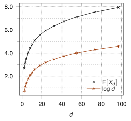
(a) Comparison of computed value of $E{[X_{d}]}$ with ${\log d}$ (Lemma 6.2).

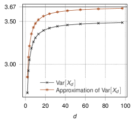
(b) Comparison of computed value of $Var{[X_{d}]}$ with approximation (Lemma 6.2).

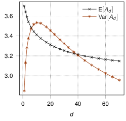
(c) $E{[A_{d}]}$ and $Var{[A_{d}]}$ from Lemma 6.9.

Figure 3: Comparisons of computed with approximated values from Lemma 6.2 and 6.9.

6.2 Memory Corruption

This section considers the case that the memory of a single node $v$ is corrupted. First consider the case that the fault causes variable $v.final$ to change to $false$. If $v.c$ does not change, then a legitimate configuration is reached after one round. So assume $v.c$ also changes. Then the fault will not affect other nodes. This is because no $w\in N(v)$ will change its value of $w.c$ because $w.final=true$ and $v.final=false$. Thus, with probability at least $1/2$ node $v$ will choose in the next round a color different form the colors of all neighbors and terminate one round later. Similar to $X_{d}$ let random variable $Z_{d}$ denote the number of rounds until a legal coloring is reached ($d=|N_{conf}(v)|$). It is easy to verify that $E[Z_{d}]=3$ in this case.

The more interesting case is that only variable $v.c$ is affected (i.e. $v.final$ remains $true$). Let $c_{f}$ the corrupted value of $v.c$ and suppose that $N_{conf}(v)=\{w\in N(v)\mid w.c=c_{f}\}\not=\emptyset$. A node not contained in $S=N_{conf}(v)\cup\{v\}$ will not change its state (c.f. Lemma 6.1). Thus, the contamination radius is $1$ and at most $\delta_{i}(v)+1$ nodes change their state. Let $d=|N_{conf}(v)|$. The subgraph $G_{S}$ induced by $S$ is a star graph with $d+1$ nodes and center $v$.

Lemma 6.7

To find a lower bound for $E[Z_{d}]$ we may assume that $w$ can choose a color from $\{0,1\}\backslash tabu$ with $tabu=\emptyset$ if $v.final=false$ and $tabu=\{v.c\}$ otherwise and $v$ can choose a color from $\{0,1,\ldots,d\}\backslash tabu$ with $tabu\subseteq\{0,1\}$.

• When a node $u\in S$ chooses a color with function randomColor the color is randomly selected form $C_{u}=\{0,1,\ldots,\delta(v)\}\backslash tabu$. Thus, if $w$ and $v$ choose colors in the same round, the probability that the chosen colors coincide is

  $$\frac{|C_{w}\cap C_{v}|}{|C_{w}||C_{v}|}.$$

  This value is maximal if $|C_{w}\cap C_{v}|$ is maximal and $|C_{w}||C_{v}|$ is minimal. This is achieved when $C_{w}\subseteq C_{v}$ and $C_{v}$ is minimal (independent of the size of $C_{w}$) or vice versa. Thus, without loss of generality we can assume that $C_{w}\subseteq C_{v}$ and both sets are minimal. Thus, for $w\in N_{conf}(v)$ the nodes in $N(w)\backslash\{v\}$ already use all colors from $\{0,1,\ldots,\delta(v)\}$ but $0$ and $1$ and all nodes in $N(v)\backslash N_{conf}(v)$ already use all colors from $\{0,1,\ldots,\delta(v)\}$ but $0,1,\ldots,k$. Hence, a node $w\in N_{conf}(v)$ can choose a color from $\{0,1\}\backslash tabu$ with $tabu=\emptyset$ if $v.final=false$ and $tabu=\{v.c\}$ otherwise. Furthermore, $v$ can choose a color from $\{0,1,\ldots,k\}\backslash tabu$ with $tabu\subseteq\{0,1\}$. In this case $tabu=\emptyset$ if $w.final=false$ for all $w\in N_{conf}(v)$.

Thus, in order to bound the expected number of rounds to reach a legitimate state after a memory corruption we can assume that $G=G_{S}$ and $u.final=true$ and $w.c=0$ (i.e. $c_{f}=0$) for all $u\in S$. After one round $u.final=false$ for all $u\in S$. To compute the expected number of rounds to reach a legitimate state an execution of the algorithm for the graph $G_{s}$ is modeled by a Markov chain ${\cal M}$ with the following states ($I$ is the initial state).

$I$:

Represents the faulty state with $u.c=0$ and $u.final=true$ for all $u\in S$.

$C^{i}$:

Node $v$ and exactly $d-i$ non-center nodes will not be in a legitimate state after the following round ($0\leq i\leq d$). In particular $v.final=false$ and $w.c=v.c\not=\bot$ or $v.c=w.c=\bot$ for exactly $d-i$ non-center nodes $w$.

$P$:

Node $v$ has not reached a legitimate state but will do so in the next round. In particular $v.final=false$ and $v.c\not=w.c$ for all non-center nodes $w$.

$F$:

Node $v$ is in a legitimate state, i.e. $v.final=true$ and $v.c\not=w.c$ for all non-center nodes $w$, but $w.c$ may be equal to $\bot$.

${\cal M}$ is an absorbing chain with $F$ being the single absorbing state. Note that when the system is in state $F$, then it is not necessarily in a legitimate state. This state reflects the set of configurations considered in the last section.

Lemma 6.8

The transition probabilities of ${\cal M}$ are as follows:

$I\longrightarrow P$:

$\frac{d-1}{2d}+\frac{1}{d}\left(\frac{1}{2}\right)^{d+1}$

$I\longrightarrow C^{0}$:

$\frac{d-1}{d}\left(\frac{1}{2}\right)^{d+1}+\frac{1}{2d}$

$I\longrightarrow C^{j}$:

$\binom{d}{d-j}\left(\frac{1}{2}\right)^{d+1}$ ($0<j\leq d$)

$C^{i}\longrightarrow C^{j}$:

$\binom{d-i}{d-j}\left(\frac{1}{2}\right)^{d-i+1}+\frac{1}{d-i+1}\binom{d-i}{j-i}\left(\frac{1}{4}\right)^{d-i}(3^{d-j}-2^{d-j})$ ($0\leq i\leq j\leq d$)

$C^{i}\longrightarrow P$:

$\frac{1}{d-i+1}\left(\frac{3}{4}\right)^{d-i}+\frac{d-i-1}{2(d-i+1)}$ ($0\leq i<d$)

$C^{d}\longrightarrow P$:

$1/2$

$P\longrightarrow F$:

$1$

• We consider each case separately.

$I\longrightarrow P:$

Note that $u.final=true$ and $u.c=0$ for all $u\in S$.
Case 0: $v.c=\bot$. Impossible.
Case 1: $v.c=0$. Impossible, since non-center nodes have $c=0$ and $final=true$.
Case 2: $v.c=1$. This happens with probability $\frac{1}{2d}$. All non-center nodes $w$ choose $w.c=\bot$, this happens with probability $\left(\frac{1}{2}\right)^{d}$.
Case 3: $v.c>1$. This happens with probability $\frac{d-1}{2d}$. Non-center nodes can make any choice. This gives the total probability for this transition as $\frac{d-1}{2d}+\frac{1}{d}\left(\frac{1}{2}\right)^{d+1}.$

$I\longrightarrow C^{0}:$

Note that $u.final=true$ and $u.c=0$ for all $u\in S$.
Case 0: $v.c=\bot$. Non-center nodes choose $c=\bot$. Case has probability $\left(\frac{1}{2}\right)^{d+1}$
Case 1: $v.c=0$. Impossible (see transition $I\longrightarrow P$).
Case 2: $v.c=1$. At least one non-center nodes $w$ choose $w.c=1$, all others choose $w.c=\bot$. This case has probability $\frac{1}{2d}\sum_{l=1}^{d}\binom{d}{l}\left(\frac{1}{2}\right)^{d}=\frac{1}{2d}\left(\frac{1}{2}\right)^{d}(2^{d}-1)$
Case 3: $v.c>1$. This case is impossible.

$I\longrightarrow C^{j}:$

Note that $u.final=true$ for all $u\in S$.
Case 1: $v.c=0$. This happens with probability $1/2(d-i+1)$. None of the $d-i$ non-center nodes $w$ sets $w.c=0$, this has probability $\left(\frac{3}{4}\right)^{d-i}$
Case 2: $v.c=1$. Similar to case 1.
Case 3: $v.c>1$. (requires $d-i>1$). This happens with probability $\frac{d-i-1}{2(d-i+1)}$. Non-center nodes can make any choice.

$C^{i}\longrightarrow P:$

Note that $u.final=false$ for all $u\in S$.
Case 1: $v.c=0$. This happens with probability $1/2(d-i+1)$. None of the $d-i$ non-center nodes $w$ sets $w.c=0$, this has probability $\left(\frac{3}{4}\right)^{d-i}$
Case 2: $v.c=1$. Similar to case 1.
Case 3: $v.c>1$. This happens with probability $\frac{d-i-1}{2(d-i+1)}$. Note $d>i$. Non-center nodes can make any choice.

$C^{i}\longrightarrow C^{j}:$

Note that $u.final=false$ for all $u\in S$.
Case 1: $v.c=\bot$. This happens with probability $\frac{1}{2}$. $d-j$ non-center nodes choose $c=\bot$ (with probability $\left(\frac{1}{2}\right)^{d-j}$), the other $j-i$ non-center nodes choose $c\not=\bot$ (with probability $\left(\frac{1}{2}\right)^{j-i}$). The total probability for this case is $\binom{d-i}{d-j}\left(\frac{1}{2}\right)^{d-i+1}$.
Case 2: $v.c=0$. This happens with probability $\frac{1}{2(d-i+1)}$. Exactly $j-i$ non-center nodes choose $c=1$ (with probability $\left(\frac{1}{4}\right)^{j-i}$), $1\leq l\leq d-j$ non-center nodes choose $c=0$ (with probability $\left(\frac{1}{4}\right)^{l}$) and all other non-center nodes choose $c=\bot$ (with probability $\left(\frac{1}{2}\right)^{d-j-l}$). The total probability for this case is

$$\frac{1}{2(d-i+1)}\binom{d-i}{j-i}\left(\frac{1}{4}\right)^{j-i}\sum_{l=1}^{d-j}\binom{d-j}{l}\left(\frac{1}{4}\right)^{l}\left(\frac{1}{2}\right)^{d-j-l} =$$

$$\frac{1}{2(d-i+1)}\binom{d-i}{j-i}\left(\frac{1}{4}\right)^{j-i}\sum_{l=1}^{d-j}\binom{d-j}{l}\left(\frac{1}{2}\right)^{d-j+l} =$$

$$\frac{1}{2(d-i+1)}\binom{d-i}{j-i}\left(\frac{1}{4}\right)^{j-i}\left(\frac{1}{2}\right)^{d-j}\sum_{l=1}^{d-j}\binom{d-j}{l}\left(\frac{1}{2}\right)^{l} =$$

$$\frac{1}{2(d-i+1)}\binom{d-i}{j-i}\left(\frac{1}{2}\right)^{d+j-2i}\sum_{l=1}^{d-j}\binom{d-j}{l}\left(\frac{1}{2}\right)^{l} =$$

$$\frac{1}{2(d-i+1)}\binom{d-i}{j-i}\left(\frac{1}{2}\right)^{d+j-2i}\left(\left(\frac{3}{2}\right)^{d-j}-1\right) =$$

$$\frac{1}{2(d-i+1)}\binom{d-i}{j-i}\left(\frac{1}{4}\right)^{d-i}\left(3^{d-j}-2^{d-j}\right)$$

Case 2: $v.c=1$. Similar to Case 1.
Case 3: $v.c>0$. This does not lead to $C^{j}$ but to $P$.

We first calculate the expected number $E[A_{d}]$ of rounds to reach the absorbing state $F$. With Lemma 6.2 this will enable us to compute the expected number $E[Z_{d}]$ of rounds required to reach a legitimate system state. To build the transition matrix $P$ of ${\cal M}$ the $d+4$ states are ordered as

$$I,C^{0},C^{1},\ldots,C^{d},P,F$$

Let $Q$ be the $(d+3)\times(d+3)$ upper left submatrix of $P$. For $s=-1,0,1,\ldots,d+1$ denote by $Q_{s}$ the $(s+2)\times(s+2)$ lower right submatrix of $Q$, i.e. $Q=Q_{d+1}$. Denote by $N_{s}$ the fundamental matrix of $Q_{s}$ (notation as introduced in section 4.1). Let $1_{s}$ be the column vector of length $(s+2)$ whose entries are all $1$ and $\epsilon_{s}=N_{s}1_{s}$. For $s=0,\ldots,d$ is $\epsilon_{s}$ the expected number of rounds to reach state $F$ from state $C^{s}$ and $\epsilon_{d+1}$ is the expected number of rounds to reach state $F$ from $I$, i.e. $\epsilon_{d+1}=E[A_{d}]$ (Theorem 3.3.5, [16]).

Lemma 6.9

The expected number $E[A_{d}]$ of rounds to reach $F$ from $I$ is less than $5$ and the variance is less than $3.6$.

• Note that $Q_{s}$ and $N_{s}$ are upper triangle matrices. Let

  $$E_{i}-Q_{i}=\left(\begin{array}[]{cccc}1-a_{1}&-a_{2}&\ldots&-a_{i+2}\\ \\[-9.0pt] 0&\lx@intercol\hfil\hbox{\multirowsetup\Large$E_{i-1}-Q_{i-1}$}\hfil\lx@intercol\\[-4.0pt] \vdots&\\ 0&\end{array}\right)\hskip 25.60747ptN_{i}=\left(\begin{array}[]{cccc}x_{1}&x_{2}&\ldots&x_{i+2}\\ \\[-9.0pt] 0&\lx@intercol\hfil\hbox{\multirowsetup\Large$N_{i-1}$}\hfil\lx@intercol\\[-4.0pt] \vdots&\\ 0&\end{array}\right)$$

  $E_{i}=(E_{i}-Q_{i})N_{i}$ gives rise to $(i+2)^{2}$ equations. Summing up the $i+2$ equations for the first row of $E_{i}$ results in

  $$\epsilon_{i}=(1-a_{1})^{-1}\left(1+\sum_{l=2}^{i+2}a_{l}\epsilon_{i+1-l}\right)$$ (1)

  It is straightforward to verify that $\epsilon_{-1}=1$ and $\epsilon_{0}=3$. Hence

  $$\epsilon_{i}=(1-a_{1})^{-1}\left(1+\sum_{l=2}^{i}a_{l}\epsilon_{i+1-l}+3a_{i+1}+a_{i+2}\right)$$

  Next we show by induction on $i$ that $\epsilon_{i}\leq 4$ for $i=-1,0,1,\ldots,d$. So assume that $\epsilon_{l}\leq 4$ for $l=-1,0,1,\ldots,i-1$ with $i<d$. Then

  $$\epsilon_{i}\leq(1-a_{1})^{-1}\left(1+4\sum_{l=2}^{i}a_{l}+3a_{i+1}+a_{i+2}\right)$$

  since $a_{i}\geq 0$. Using the fact $1-a_{1}=\sum_{l=2}^{i+2}a_{l}$ this inequality becomes

  $$\epsilon_{i} \leq (1-a_{1})^{-1}(1+4(1-a_{1}-a_{i+1}-a_{i+2})+3a_{i+1}+a_{i+2})=4+\frac{1-a_{i+1}-3a_{i+2}}{1-a_{1}}$$

  Coefficient $a_{j}$ denotes the transition probability from $C^{d-i}$ to $C^{d+j-(i+1)}$ for $j=1,\ldots,i+1$ and $a_{i+2}$ that for changing from $C^{d-i}$ to $P$. For $i\leq d$ the following values from Lemma 6.8 are used:

  $$a_{1} = \left(\binom{i}{i+1-l}\left(\frac{1}{2}\right)^{i+1}+\frac{1}{i+1}\binom{i}{l-1}\left(\frac{1}{4}\right)^{i}(3^{i+1-l}-2^{i+1-l})\right)$$

  $$a_{i+1} = \left(\frac{1}{2}\right)^{i+1}\text{ and }a_{i+2}=\frac{1}{i+1}\left(\frac{3}{4}\right)^{i}+\frac{i-1}{2(i+1)}.\text{ \leavevmode\nobreak\ Thus,}$$

  $$3a_{i+2}=\frac{3}{i+1}\left(\frac{3}{4}\right)^{i}+\frac{3(i-1)}{2(i+1)}>1$$

  holds for $i\geq 2$. This yields

  $$\frac{1-a_{i+1}-3a_{i+2}}{1-a_{1}}<0$$

  and therefore $\epsilon_{i}\leq 4$. To bound $\epsilon_{d+1}$ we use Equation 1 with $i=d+1$. Note that in this case $a_{1}=0$ since a transition from $I$ to itself is impossible. Hence

  $$E[A_{d}]=\epsilon_{d+1}=1+\sum_{l=2}^{d+3}a_{l}\epsilon_{d+2-l}\leq 1+4\sum_{l=2}^{d+3}a_{l}=5$$

  Thus, $Var[A_{d}]=((2N_{d+1}-E_{d+1})1_{d+1}-1_{d+1}^{2})[1]=2\sum_{i=1}^{d+3}x_{i}\epsilon_{d+2-i}-\epsilon_{d+1}-\epsilon_{d+1}^{2}$ Fig. 3(c) shows that $Var[A_{d}]\leq 3.6$.

Lemma 6.10

The expected value for the containment time after a memory corruption at node $v$ is at most $\frac{1}{\ln 2}H_{\delta_{i}(v)}+11/2$ with variance less than $7.5$.

• For a set $X$ of configurations and a single system configurations $c$ denote by $E(c,X)$ the expected value for the number of transitions from $x$ to a state in $X$. Denote by ${\cal L}$ the set of legitimate system states. Then

  $$E(I,{\cal L}) = \sum_{e\in T(I,{\cal L})}l(e)p(e)$$

  $$= \sum_{x\in F}\sum_{e_{1}\in T(I,x)}\sum_{e_{2}\in T(x,{\cal L})}(l(e_{1})+l(e_{2}))p(e_{1})p(e_{2})$$

  $$= \sum_{x\in F}\sum_{e_{1}\in T(I,x)}\left(l(e_{1})p(e_{1})\sum_{e_{2}\in T(x,{\cal L})}p(e_{2})+p(e_{1})\sum_{e_{2}\in T(x,{\cal L})}l(e_{2})p(e_{2})\right)$$

  $$= \sum_{x\in F}\sum_{e_{1}\in T(I,x)}\left(l(e_{1})p(e_{1})+p(e_{1})E(x,{\cal L})\right)$$

  $$= \sum_{x\in F}\left(E(I,x)+\sum_{e_{1}\in T(I,x)}p(e_{1})E(x,{\cal L})\right)$$

  $$\leq E(I,F)+\max\{E(x,{\cal L})\mid x\in F\}\sum_{e_{1}\in T(I,F)}p(e_{1})$$

  $$= E(I,F)+\max\{E(x,{\cal L})\mid x\in F\}\leq 5+\frac{1}{\ln 2}H_{\delta_{i}(v)}+1/2$$

  The last step uses Lemma 6.9 and 6.2. The bound on the variance is proved similarly.

Theorem 5.1, Lemma 6.10, 6.2, and 6.1 prove the following Theorem.

Theorem 6.11

${\cal A}_{col}$ is a self-stabilizing algorithm for computing a $(\Delta+1)$-coloring in the synchronous model within $O(\log n)$ time with high probability. It uses messages of size $O(\log n)$ and requires $O(\log n)$ storage per node. With respect to memory and message corruption it has contamination radius $1$. The expected containment time is at most $\frac{1}{\ln 2}H_{\Delta_{i}}+11/2$ with variance less than $7.5$.

Corollary 6.12

Algorithm ${\cal A}_{col}$ has expected containment time $O(1)$ for bounded-independence graphs. For unit disc graphs this time is at most $8.8$.

• For these graphs $\Delta_{i}\in O(1)$, in particular $\Delta_{i}\leq 5$ for unit disc graphs.

7 Conclusion

This paper presented techniques to derive upper bounds for the mean time to recover of a single fault for self-stabilizing algorithms in the synchronous message passing model. For a new $\Delta+1$-coloring algorithm we analytically derive a bound of $\frac{1}{\ln 2}H_{\Delta_{i}}+11/2$ for the expected containment and showed that the variance less than $7.5$. We believe that the technique can also be applied to other self-stabilizing algorithms.

Acknowledgments

Research was funded by Deutsche Forschungsgemeinschaft DFG (TU 221/6-1).

References

- [1] Yossi Azar, Shay Kutten, and Boaz Patt-Shamir. Distributed error confinement. ACM Trans. Algorithms, 6(3):48:1–48:23, 2010.
- [2] Leonid Barenboim and Michael Elkin. Distributed Graph Coloring: Fundamentals and Recent Developments. Morgan & Claypool Publishers, 2013.
- [3] Joffroy Beauquier, S. Delaet, and S. Haddad. Necessary and sufficient conditions for 1-adaptivity. In 20th Int. Parallel & Distr. Processing Symp., pages 10–16, 2006.
- [4] P. Crouzen, E.M. Hahn, H. Hermanns, A. Dhama, O. Theel, R. Wimmer, B. Braitling, and B. Becker. Bounded fairness for probabilistic distributed algorithms. In 11th Int. Conf. Appl. of Concurrency to System Design, pages 89–97, June 2011.
- [5] Robert DeVille and Sayan Mitra. Stability of distributed algorithms in the face of incessant faults. In Proc. SSS 09, volume 5873 of LNCS, pages 224–237. Springer, 2009.
- [6] Shlomi Dolev. Self-Stabilization. MIT Press, 2000.
- [7] Shlomi Dolev and Ted Herman. Superstabilizing protocols for dynamic distributed systems. Chicago J. Theor. Comput. Sci., 4:1–40, 1997.
- [8] Swan Dubois, Toshimitsu Masuzawa, and Sebastien Tixeuil. Bounding the impact of unbounded attacks in stabilization. IEEE Trans. on Parallel & Distr. Systems, 23(3):460–466, 2012.
- [9] Marie Duflot, Laurent Fribourg, and Claudine Picaronny. Randomized finite-state distributed algorithms as markov chains. In Distr. Comp., volume 2180 of LNCS, pages 240–254. 2001.
- [10] Laurent Fribourg, Stéphane Messika, and Claudine Picaronny. Coupling and self-stabilization. Distributed Computing, 18(3):221–232, February 2006.
- [11] Felix C. Gärtner. Fundamentals of fault-tolerant distributed computing in asynchronous environments. ACM Comput. Surv., 31(1):1–26, 1999.
- [12] Sukumar Ghosh, Arobinda Gupta, Ted Herman, and SriramV. Pemmaraju. Fault-containing self-stabilizing distributed protocols. Distributed Computing, 20(1):53–73, 2007.
- [13] Sukumar Ghosh and Xin He. Scalable self-stabilization. J. Parallel Distrib. Comput., 62(5):945–960, 2002.
- [14] Maria Gradinariu and Sebastien Tixeuil. Self-stabilizing vertex coloring of arbitrary graphs. In 4th Int. Conf. on Princ. of Distributed Systems, OPODIS’2000, pages 55–70, 2000.
- [15] Öjvind Johansson. Simple Distributed -coloring of Graphs. Inf. Process. Lett., 70(5):229–232, 1999.
- [16] J. G. Kemmeny and J. L. Snell. Finite Markov Chains. Springer Press, 1976.
- [17] Sven Köhler and Volker Turau. Fault-containing self-stabilization in asynchronous systems with constant fault-gap. Distributed Computing, 25(3):207–224, 2012.
- [18] Shay Kutten and Boaz Patt-Shamir. Adaptive stabilization of reactive protocols. In FSTTCS, volume 3328 of LNCS, pages 396–407. Springer, 2004.
- [19] Michael Luby. A simple parallel algorithm for the maximal independent set problem. SIAM J. Comput., 15(4):1036–1055, 1986.
- [20] Nathalie Mitton, Eric Fleury, Isabelle Guérin-Lassous, Bruno Séricola, and Sébastien Tixeuil. On Fast Randomized Colorings in Sensor Networks. In Proc. ICPADS, pages 31–38. IEEE, 2006.
- [21] Mikhail Nesterenko and Anish Arora. Tolerance to unbounded byzantine faults. In Proc. 21st Symposium on Reliable Distributed Systems, pages 22–29, 2002.
- [22] David Peleg. Distributed Computing: A Locality-Sensitive Approach. SIAM Society for Industrial and Applied Mathematics, Philadelphia, 2000.
- [23] Masafumi Yamashita. Probabilistic self-stabilization and random walks. 2013 Int. Conf. on Computing, Networking and Communications (ICNC), pages 1–7, 2011.