Are Spine–Sheath Polarization Structures in the Jets of Active Galactic Nuclei Associated with Helical Magnetic Fields?

Abstract

One possible origin for polarization structures across jets of Active Galactic Nuclei (AGNs) with a central “spine” of orthogonal magnetic field and a “sheath” of longitudinal magnetic field along one or both edges of the jet is the presence of a helical jet magnetic field. Simultaneous Very Long Baseline Array (VLBA) polarization observations of AGN displaying partial or full spine–sheath polarization structures were obtained at 4.6, 5.0, 7.9, 8.9, 12.9 and 15.4 GHz, in order to search for additional evidence for helical jet magnetic fields, such as transverse Faraday rotation gradients (due to the systematic change in the line-of-sight magnetic-field component across the jet). Results for eight sources displaying monotonic transverse Faraday rotation gradients with significances $\geq 3\sigma$ are presented here. Reversals in the directions of the transverse RM gradients with distance from the core or with time are detected in three of these AGNs. These can be interpreted as evidence for a nested helical magnetic field structure, with different directions for the azimuthal field component in the inner and outer regions of helical field. The results presented here support the idea that many spine–sheath polarization structures reflect the presence of helical magnetic fields being carried by these jets.

1 Introduction

The radio emission associated with Active Galactic Nuclei (AGNs) is synchrotron emission, which can be linearly polarized up to about 75% in optically thin regions, where the polarization angle $\chi$ is orthogonal to the projection of the magnetic field B onto the plane of the sky, and up to 10–15% in optically thick regions, where $\chi$ is parallel to the projected B (Pacholczyk 1970). Linear polarization measurements thus provide direct information about both the degree of order and the direction of the B field giving rise to the observed synchrotron radiation.

Table 1: Source properties
Source	Redshift	pc/mas	Integrated Faraday Rotation	Reference
			(rad/m2)
0333+321	1.259	8.41	$56\pm 10$	Rusk (1988)
0738+313	0.631	6.83	$12\pm 10$	Simard–Normandin et al. (1981)
0836+710	2.218	8.37	$-9\pm 3$	Rusk (1988)
0923+392	0.695	7.12	$15\pm 24$	Rusk (1988)
1150+812	1.25	8.40	$107\pm 8$	Rusk (1988)
1633+382	1.813	8.54	$4\pm 4$	Rusk (1988)
2037+511	1.686	8.56	$-29\pm 6$	Rusk (1988)
2345$-$167	0.576	6.54	$-0.5\pm 1.1$	Taylor et al. (2009)

Multi-frequency Very Long Baseline Interferometry (VLBI) polarization observations also provide information about the parsec-scale distribution of the spectral index (optical depth) of the emitting regions, as well as Faraday rotation occurring between the source and observer. Faraday rotation of the plane of linear polarization occurs during the passage of the associated electromagnetic wave through a region with free electrons and a B field with a non-zero component along the line of sight. When the Faraday rotation occurs outside the emitting region in regions of non-relativistic (“thermal”) plasma, the amount of rotation is given by

$$\chi_{obs}-\chi_{o}=\frac{e^{3}\lambda^{2}}{8\pi^{2}\epsilon_{o}m^{2}c^{3}}\int n_{e}{\mathbf{B}}\cdot d{\mathbf{l}}\equiv RM\lambda^{2}$$ (1)

where $\chi_{obs}$ and $\chi_{o}$ are the observed and intrinsic polarization angles, respectively, $-e$ and $m$ are the charge and mass of the particles giving rise to the Faraday rotation, usually taken to be electrons, $c$ is the speed of light, $n_{e}$ is the density of the Faraday-rotating electrons, $\mathbf{B}$ is the magnetic field, $d\mathbf{l}$ is an element along the line of sight, $\lambda$ is the observing wavelength, and RM (the coefficient of $\lambda^{2}$) is the Rotation Measure (e.g., Burn 1966). Simultaneous multifrequency observations thus allow the determination of both the RM, which carries information about the electron density and the line-of-sight B field in the region of Faraday rotation, and $\chi_{o}$, which carries information about the intrinsic B-field geometry associated with the source projected onto the plane of the sky.

Systematic gradients in the Faraday rotation have been reported across the parsec-scale jets of several AGN, interpreted as reflecting the systematic change in the line-of-sight component of a toroidal or helical jet B field across the jet (e.g. Hovatta et al. 2012, Mahmud et al. 2013, Gabuzda et al. 2014). Such fields would come about in a natural way as a result of the “winding up” of an initial “seed” field by the rotation of the central accreting objects (e.g. Nakamura, Uchida & Hirose 2001; Lovelace et al. 2002).

The first AGN jet found to display polarization structure with a central “spine” of longitudinal polarization (orthogonal magnetic field) with a “sheath” of orthogonal polarization (longitudinal magnetic field) along the edges of the jet was 1055+018; Attridge et al. (1999) proposed that interaction with the surrounding medium caused the “sheath” and transverse shocks propagating along the jet caused the “spine”. Since the discovery of this first example, a number of other AGN displaying this type of magnetic field structure have been identified (e.g. Pushkarev et al. 2005), suggesting that the conditions giving rise to this magnetic-field structure are not uncommon. It has also been pointed out that such polarization structure could reflect the presence of an overall helical magnetic field associated with the jet (Lyutikov et al. 2005, Pushkarev et al. 2005): in projection onto the plane of the sky, the predominant component of a helical or toroidal field associated with a roughly cylindrical length of jet will be orthogonal near the central part of the jet and become longitudinal near the jet edges.

Although it may be difficult to conclusively demonstrate which of these pictures is correct in any individual AGN, one way to try to distinguish between these two scenarios is to search for additional evidence for the presence of helical jet magnetic fields in AGN displaying spine–sheath or similar polarization structures, most notably transverse Faraday rotation gradients. Another possible sign of a helical jet magnetic field is a systematic rise in the degree of polarization toward one or both edges of the jet, compared to the degree of polarization near the jet ridge line. This comes about because the degree of polarization depends on the magnetic-field component in the plane of the sky, which will be enhanced toward the edges of a jet carrying a helical magnetic field.

Figure 1: Intensity maps with polarization angles superposed: (a) 0333+321, peak 0.701 Jy, minimum polarized flux plotted 1.25 mJy; (b) 0738+313, peak 0.930 Jy, minimum polarized flux plotted 0.80 mJy; (c) 0836+710, peak 0.828 Jy, minimum polarized flux plotted 1.00 mJy; (d) 0923+392, peak 8.750 Jy, minimum polarized flux plotted 30 mJy. In all cases, the the maps are at 7.9 GHz, and the contours shown are $-0.125$, 0.125, 0.25, 0.50, 1, 2, 4, 8, 16, 32, 64 and 95% of the peak. The beam size is shown in the lower left corner of each map.

Figure 2: Intensity maps with polarization angles superposed: (a) 1150+812, peak 1.058 Jy, minimum polarized flux plotted 3.0 mJy; (b) 1633+382, peak 1.517 Jy, minimum polarized flux plotted 2.8 mJy; (c) 2037+511, peak 1.955 Jy, minimum polarized flux plotted 1.7 mJy; (d) 2345$-$167, peak 1.210 Jy, minimum polarized flux plotted 2.6 mJy. The maps of 1150+812, 1633+382 and 2345$-$167 are at 7.9 GHz, and the map of 2037+511 is at 8.9 GHz. In all cases, the contours shown are $-0.125$, 0.125, 0.25, 0.50, 1, 2, 4, 8, 16, 32, 64 and 95% of the peak. The beam size is shown in the lower left corner of each map.

With this aim, simultaneous Very Long Baseline Array (VLBA) polarization observations of 22 AGN displaying full or partial spine–sheath polarization structures in earlier MOJAVE observations (Monitoring of Jets in Active galactic nuclei with VLBA Experiments; http://www.physics.purdue.edu/MOJAVE/) were obtained at 4.6, 5.0, 7.9, 8.9, 12.9 and 15.4 GHz, in two 24-hour sessions, on September 26 and 27, 2007 (VLBA projects BG173A and BG173B, respectively). We consider here results for eight of these objects observed in the latter of these two sessions.

2 Observations and Reduction

The observations analyzed here were obtained on September 27, 2007 (project BG173B) with all ten antennas of the VLBA except for Saint Croix, which could not participate due to bad weather. The frequencies observed were 4.612, 5.092, 7.916, 8.883, 12.939 and 15.383 GHz. All of the frequencies except for 4.6 and 5.0 GHz were built up of four intermediate frequencies (IFs) per polarization, each 8-MHz wide, making a total frequency bandwidth of 32 MHz per polarization. In the case of 4.6 and 5.0 GHz, the total bandwidth used was split between these two frequencies, so that each was observed at 16-MHz per polarization.

Ten AGNs whose jets displayed signs of spine–sheath polarization structures in earlier MOJAVE obserations were observed in this session, together with 0851+202, which was observed as a calibrator. Each source was observed for a total of 25–30 minutes at each frequency, in a “snap-shot” mode with 8–10 scans spread out over the total time the source was observable with all or most of the VLBA antennas. The total duration of the VLBI observations was about 24 hours. Eight of the ten targets observed in our September 27, 2007 session (BG173B) showed evidence for statistically significant transverse Faraday-rotation gradients across their core-regions and/or jets, and it is these eight sources that we consider here (Table 1).

The preliminary phase and amplitude calibration, polarization (D-term) calibration, electric vector position angle (EVPA) calibration and imaging were all carried out in the National Radio Astronomy Observatory (NRAO) AIPS package using standard techniques. The reference antenna used was Los Alamos (LA).

The instrumental polarizations (D-terms) were derived using the AIPS task LPCAL, using the compact polarized source 0851+202 with good parallactic angle coverage, solving simultaneously for the source polarizations in a small number of individual VLBI components corresponding to groups of CLEAN components, identified by hand. To check the solutions, the D-terms for each of the four IFs were checked for consistency at each station, and plots of the real against the imaginary cross-hand polarization data were used to verify the successful removal of the D-terms.

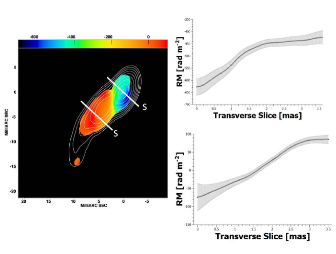
Figure 3: 4.6-GHz intensity map of 0333+321 with the RM distribution superposed (left). The contours shown are $-0.25$, 0.25, 0.50, 1, 2, 4, 8, 16, 32, 64 and 95% of the peak of 1.05 Jy/beam. The convolving beam is 3.8 mas $\times$ 2.0 mas in position angle $-20^{\circ}$. The lines drawn across the RM distribution show the locations of the RM slices shown in the corresponding right-hand panels; the letter “S” at one end of these lines marks the side corresponding to the starting point for the slice.

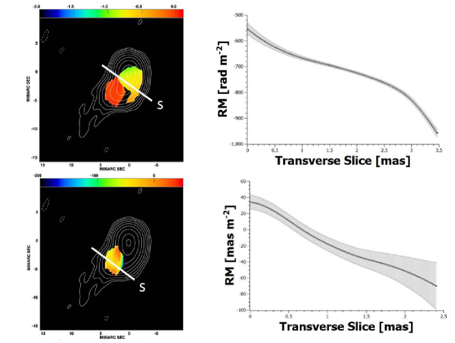
Figure 4: 4.6-GHz intensity map of 0738+318 with the RM distributions superposed (left). The contours shown are $-0.25$, 0.25, 0.50, 1, 2, 4, 8, 16, 32, 64 and 95% of the peak of 1.04 Jy/beam. The convolving beam is 3.9 mas $\times$ 2.0 mas in position angle $-15^{\circ}$. The colour scales for the upper and lower RM maps have been chosen to highlight the transverse gradients in the core and jet regions, respectively. The lines drawn across the RM distributions show the locations of the RM slices shown in the corresponding right-hand panels; the letter “S” at one end of these lines marks the side corresponding to the starting point for the slice.

To calibrate the electric vector position angles (EVPAs), we used integrated polarization measurements of 0851+202 from the Very Large Array (VLA) polarization monitoring program, as well as the 26-m radio telescope of the University of Michigan Radio Astronomy Observatory (UMRAO). The closest VLA polarization observations of 0851+202 were obtained on the 29th September 2007 (5, 8.5, 22 and 43 GHz), and the closest UMRAO observations were from the 25th September 2007 (14.5 GHz), 28th September 2007 (4.8 GHz) and 3rd October 2007 (8 GHz). Fortunately, all these integrated measurements were within a few days of the VLBA observations, minimizing the probability of source variability between the VLBA and integrated measurements. Since the integrated Faraday rotation measure of 0851+202 is modest ($+31$ rad/m²; Rudnick & Jones 1983), the differences in the EVPA between the nearest integrated and VLBA frequencies were negligible. The VLA and UMRAO integrated polarization angles gave consistent results. The rotations required for the EVPA calibration were $\Delta\chi=105^{\circ},96^{\circ},82^{\circ},87^{\circ},62^{\circ},$ and $89^{\circ}$ at 4.6, 5.0, 7.9, 8.9, 12.9 and 15.4 GHz, respectively. We estimate that the uncertainty in these EVPA calibrations is no worse than $3^{\circ}$ at each frequency.

Maps of the distribution of the total intensity $I$ and Stokes parameters $Q$ and $U$ at each frequency were made, both with natural weighting, and with matched resolutions corresponding to a specified beam, usually the lowest-frequency beam. The distributions of the polarized flux ($p=\sqrt{Q^{2}+U^{2}}$) and polarization angle ($\chi=\frac{1}{2}\arctan\frac{U}{Q}$) were obtained from the $Q$ and $U$ maps using the AIPS task COMB. Maps of the RM were then constructed using the AIPS task RM, after first subtracting the effect of the integrated RM (presumed to arise in our Galaxy) from the observed polarization angles, so that any residual Faraday Rotation was due predominantly to thermal plasma in the vicinity of the AGN. The uncertainties in the RM were based on the uncertainties in $Q$ and $U$, which were, in turn, estimated using the approach of Hovatta et al. (2012). This method is based on the results of Monte Carlo simulations, and takes into account the fact that uncertainties on-source are higher than the off-source rms fluctuations in the image. The output pixels in the RM maps were blanked when the RM uncertainty from the $\chi$ vs. $\lambda^{2}$ fit exceeded a specified value, usually in the range 50–70 rad/m².

The effect of the integrated RM is usually small, but can be substantial for some sources, e.g. those lying near the plane of the Galaxy. We used various integrated VLA RM measurements from the literature, listed in Table 1, together with other basic information about the eight sources for which results are presented here. The observations of Rusk (1988) were obtained using pointed VLA observations at 4.860 and 14.940 GHz; we used these integrated RM values when they were available, which was the case for all but two of our sources. We used the integrated RM for 2345$-$176 from Taylor et al. (2009), who measured the Faraday Rotations of 37,543 polarized radio sources based on data from the NRAO VLA Sky Survey (NVSS) at 1364.9 and 1435.1 MHz. The only source for which neither of these references provided an integrated RM was 0738+313; we used the integrated RM for this source given by Simard–Normandin et al. (1981), who published integrated rotation measures for 555 extragalactic radio sources based on polarization measurements at several wavelengths between 1.73 and 10.5 GHz. None of the objects considered here have integrated RM values large enough to substantially influence the observed polarization angles at the frequencies at which our observations were made.

3 Results

We present here polarization maps at 7.9 GHz (8.9 GHz for 2037+511) and RM maps based on all six of our frequencies for each of the eight AGNs considered in this paper. Additional polarization maps for each of the sources at 15 GHz can be found in Lister & Homan (2005) and the MOJAVE website (http://www.physics.purdue.edu/MOJAVE/). The source names, redshifts, pc/mas values and integrated rotation measures are summarized in Table 1. The redshifts and pc/mas vales were taken from the MOJAVE project website (http://www.physics.purdue.edu/MOJAVE/); the latter were determined assumed a cosmology with $H_{o}=71$ km s^-1Mpc^-1, $\Omega_{\Lambda}=0.73$ and $\Omega_{m}=0.27$.

In addition to the eight AGNs considered here, we also observed two other sources whose MOJAVE maps display signs of spine–sheath polarization structures: 1504$-$166 and 1730$-$130. However, the polarization and Faraday rotation images of these sources did not reveal any new structures, and we therefore do not consider them further here.

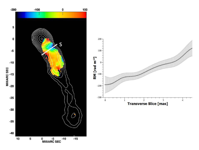
Figure 5: 4.6-GHz intensity map of 0836+710 with the RM distribution superposed (left). The contours shown are $-0.25$, 0.25, 0.50, 1, 2, 4, 8, 16, 32, 64 and 95% of the peak of 0.98 Jy/beam. The convolving beam is 2.8 mas $\times$ 2.8 mas. The line drawn across the RM distribution shows the location of the RM slice shown in the right-hand panel; the letter “S” at one end of this line marks the side corresponding to the starting point for the slice.

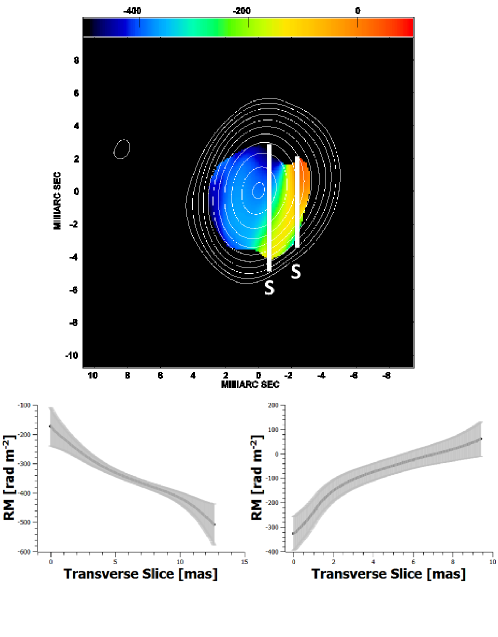
Figure 6: 4.6-GHz intensity map of 0923+392 with the RM distribution superposed (upper). The contours shown are $-0.25$, 0.25, 0.50, 1, 2, 4, 8, 16, 32, 64 and 95% of the peak of 8.40 Jy/beam. The convolving beam is 3.6 mas $\times$ 2.4 mas in position angle $-15^{\circ}$. The lines drawn across the RM distributions show the locations of the RM slices shown in the corresponding lower panels; the letter “S” at one end of these lines marks the side corresponding to the starting point for the slice.

When possible, we determined the relative shifts between the various images used to make the RM maps. In all cases, these shifts were tested by making spectral-index maps taking into account the relative shifts, to ensure that they did not show any spurious features due to residual misalignment between the maps. The relative shifts between each frequency and 15.4 GHz for each source for which these were significant are summarized in Table 2.

Table 2: Image shifts relative to 15.4 GHz (mas)
Freq (GHz)	Source
	0333+321	0836+710	2037+511
12.9	0.0	0.2	0.0
8.9	0.1	0.5	0.04
7.9	0.1	0.7	0.14
5.0	0.36	1.2	0.14
4.6	0.36	1.4	0.14

RM maps together with slices in regions of detected transverse RM gradients are also shown in Figs. 3–10. For consistency, in each case, these were taken in the clockwise direction relative to the base of the jet (located upstream from the observed core). The lines drawn across the RM distributions show the locations of the slices; the letter “S” at one end of these lines marks the side corresponding to the starting point for the slice (a slice distance of 0).

The statistical significance of transverse gradients detected in our RM maps are summarized in Table 3. When plotting the slices in Figs. 3–10 and finding the difference between the RM values at two ends of a gradient, we did not include uncertainty in the polarization angles due to EVPA calibration uncertainty; this is appropriate, since EVPA calibration uncertainty affects all polarization angles for the frequency in question equally, and so cannot introduce spurious RM gradients, as is discussed by Mahmud et al. (2009) and Hovatta et al. (2012).

3.1 0333+321

VLBA observations of 0333+321 at 8 frequencies near 4 and 8 GHz obtained in 2003 are presented by Asada et al. (2008), who found the jet EVPAs to be almost perpendicular to the jet direction and to follow the bending of the jet. Thus, they inferred the magnetic field to run roughly parallel to the jet direction. Asada et al. (2008) also reported a clear gradient in the RM distribution across the jet, which they interpreted as evidence for a helical jet magnetic field, particularly since the gradient encompassed both positive and negative values.

Figure 1a shows our 7.9 GHz polarization map for 0333+321. As observed by Asada et al. (2008), the EVPAs are generally perpendicular to the jet, in both the core and jet. The jet polarization is offset somewhat toward the southern edge of the jet.

We were able to derive reasonable relative core shifts for this source. The derived shifts relative to 15.4 GHz are given in Table 2.

Figure 3 presents the RM distribution for 0333+321 for our six frequencies, superimposed onto the 4.6 GHz intensity contours. We subtracted the integrated RM determined by Rusk (1988) before making the RM map (Table 1); this had only a modest effect on the observed angles, changing them by no more than about $12^{\circ}$. The RM maps produced directly and taking into account the small relative shifts between the frequencies were virtually identical. Our RM map confirms the presence of a clear RM gradient transverse to the jet direction along the entire jet and core region, as was reported by Asada et al. (2008). Figure 3 also shows two slices taken roughly perpendicular to the jet direction plotted together with their errors. The transverse RM gradients are all in the same direction and are monotonic. The significance of the gradients is approximately $4\sigma$.

Inspection of the RM distribution by eye gives the impression of the gradient across the jet being slanted, as is also visible in the RM map shown in Asada et al. (2008). This could be due to a combination of a transverse RM gradient across and a decreasing RM along the jet, as would be expected if there is a decrease in electron density and magnetic field strength with distance from the core.

3.2 0738+318

Figure 1b shows our 7.9 GHz polarization map for 0738+318. The EVPAs in the inner part of the jet lie along the jet, which is oriented toward the south, and become roughly transverse to the jet beyond a bend toward the east a few mas from the core. The polarization beyond this bend is offset toward the northern edge of the jet.

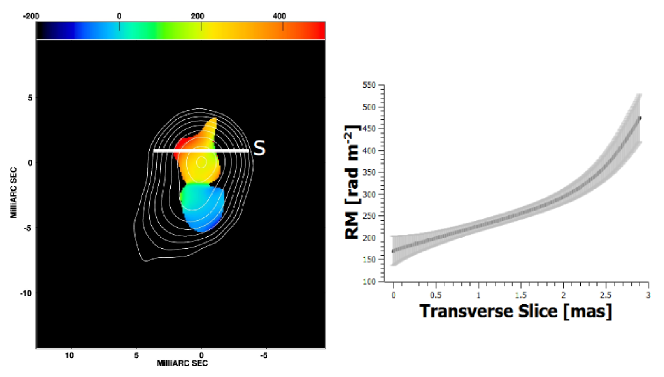
Figure 7: 4.6-GHz intensity map of 1150+812 with the RM distribution superposed (left). The contours shown are $-0.25$, 0.25, 0.50, 1, 2, 4, 8, 16, 32, 64 and 95% of the peak of 1.08 Jy/beam. The convolving beam is 2.5 mas $\times$ 2.1 mas in position angle $25^{\circ}$. The line drawn across the RM distribution shows the location of the RM slice shown in the right-hand panel; the letter “S” at one end of this line marks the side corresponding to the starting point for the slice.

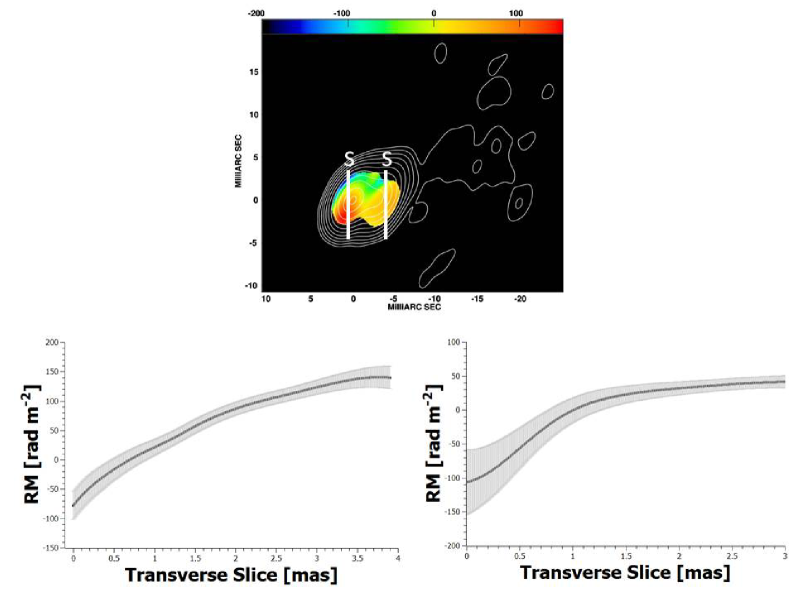
Figure 8: 4.6-GHz intensity map of 1633+382 with the RM distribution superposed (upper). The contours shown are $-0.25$, 0.25, 0.50, 1, 2, 4, 8, 16, 32, 64 and 95% of the peak of 1.30 Jy/beam. The convolving beam is 3.7 mas $\times$ 2.2 mas in position angle $-25^{\circ}$. The lines drawn across the RM distributions show the locations of the RM slices shown in the corresponding lower panels; the letter “S” at one end of these lines marks the side corresponding to the starting point for the slice.

We found no indication of appreciable shifts between the images at different frequencies. A spectral-index map produced by directly superposing the 5 and 15 GHz images does not show any significant signs of misalignment. We accordingly made the RM map for this source without attempting to apply any further image alignment.

Figure 4 presents the RM distribution for 0738+318 for our six frequencies, superimposed onto the 4.6 GHz intensity contours. We subtracted the effect of the integrated RM given by Simard–Normandin et al. (1981) (Table 1) from the observed polarization angles before making the RM map for completeness, although this had a nearly negligible effect, changing the observed angles by no more than about $2.5^{\circ}$. This RM map shows the presence of an RM gradient roughly transverse to the jet direction in the core/inner jet region. Figure 4 shows two slices taken roughly perpendicular to the jet direction plotted together with their errors. In both cases, the transverse RM gradients are in the same direction and monotonic. The significance of the transverse RM gradient in the inner of the two regions considered is approximately $15\sigma$, dropping to $3.5\sigma$ further from the core.

3.3 0836+710

VLBA observations of 0836+710 at 8 frequencies near 5 and 8 GHz obtained in 2003 are presented by Asada et al. (2010), who found the projected magnetic field to be roughly parallel to the jet direction. They also detected a clear transverse RM gradient about 3–4 mas from the core.

Figure 1c shows our 7.9 GHz polarization map for 0836+710. As observed previously, the jet EVPAs are primarily perpendicular to the jet, indicating a predominantly longitudinal magnetic field. In some places, the polarization is clearly offset from the center of the jet ridgeline; there are also some regions where the polarization sticks are oblique to the jet direction. The EVPAs in the innermost part of the jet are aligned with the jet, indicating an orthogonal magnetic field component in this region.

We were able to derive reasonable relative core shifts for this source. The derived shifts relative to 15.4 GHz are given in Table 2.

Figure 5 presents the RM distribution for 0836+710 for our six frequencies, superimposed onto the 4.6 GHz intensity contours. We subtracted the effect of the integrated RM determined by Rusk (1988) from the observed polarization angles before making the RM map (Table 1) for completeness, although this had a nearly negligible effect, changing the observed angles by no more than about $2^{\circ}$. The RM maps produced directly and taking into account the small relative shifts between the frequencies were virtually identical. Our RM map shows a clear gradient transverse to the jet roughly 5 mas from the core. Figure 5 also shows a slice taken roughly perpendicular to the jet direction plotted together with its errors. The transverse RM gradient in this region is monotonic, and has a significance of about $3\sigma$.

At first, these results seem to confirm the results of Asada et al. (2010), who observed a transverse RM gradient in approximately the same location in the jet. However, the gradient reported by Asada et al. (2010) [for data obtained in January 2003] is in the opposite direction to the one observed in our data [for data obtained in September 2007]. In fact, Mahmud et al. (2009) observed a similar flip in the direction of an RM gradient across the jet of 1803+784, which they interpreted as evidence for a picture in which the change in the direction of the RM gradient is due to a change in domination between an inner and outer region of helical magnetic field.

3.4 0923+392

Figure 1d shows our 7.9 GHz polarization map for 0923+392. Note that this represents the relatively rare case when the map peak does not correspond to the core; the core is located at the northwest end of the observed structure, whereas the jet structure extends toward the southeast [see the spectral-index maps presented by Zavala & Taylor (2003) and Hovatta et al. (2014)]. The jet EVPAs are roughly aligned with the jet near the jet ridgeline, becoming more orthogonal or oblique near the southern edge of the jet.

The core shifts between our frequencies are essentially negligible (see also Pushkarev et al. 2012), and our RM maps were derived without applying additional alignments to the input data.

Figure 6 presents the RM distribution for 0923+392 for our six frequencies, superimposed onto the 4.6 GHz intensity contours. We subtracted the effect of the integrated RM determined by Rusk (1988) from the observed polarization angles before making the RM map (Table 1) for completeness, although this had only a small effect, changing the observed angles by no more than about $3^{\circ}$. Our RM map shows a gradient transverse to the jet in the inner jet/core region (northwest end of structure), as well as a transverse gradient in the opposite direction several mas out in the jet (southeast end of structure). A similar structure is also visible in the RM map of 0923+392 presented by Zavala & Taylor (2003).

Figure 6 also shows slices taken roughly perpendicular to the jet direction plotted together with their errors. The transverse RM gradients are monotonic, and have significances of approximately $3.9\sigma$ in the inner jet/core region and $3.4\sigma$ further out in the jet.

3.5 1150+812

Figure 2a shows our 7.9 GHz polarization map for 1150+812. The jet EVPAs are roughly perpendicular to the jet and clearly offset toward the western edge of the jet, indicating a longitudinal magnetic field, while the core EVPAs are oriented roughly parallel to the jet direction, suggesting an orthogonal field.

We found no indication of appreciable shifts between the images at different frequencies. A spectral-index map produced by directly superposing the 5 and 15 GHz images does not show any significant signs of misalignment. We accordingly made the RM map for this source without attempting to apply any further image alignment.

Figure 7 presents the RM distribution for 1150+812 for our six frequencies, superimposed onto the 4.6 GHz intensity contours. We subtracted the effect of the integrated RM determined by Rusk (1988) from the observed polarization angles before making the RM map (Table 1). The core region and jet both show evidence of RM gradients transverse to the jet, in the same direction. Figure 7 also shows a slice taken roughly perpendicular to the jet direction plotted together with its errors. The line drawn across the RM map indicate the location of the slice, in the core region. This gradient is monotonic, and has a significance of approximately $5\sigma$. A transverse gradient that is essentially, but not strictly, monotonic can also be observed in the inner jet. Although our subtraction of the integrated RM value led to an appreciable overall shift in the observed RM values, this did not lead to a sign change in the RM values observed at opposite ends of the observed gradient.

3.6 1633+382

Figure 2b shows our 7.9 GHz polarization map for 1633+382. The source structure is quite compact. The jet EVPAs are offset toward the southern edge of the jet, but their orientation relative to the jet direction is not entirely clear; the jet appears to bend toward the north near the location of this polarization, and it is possible that the detected polarization corresponds to a longitudinal magnetic field at the southern edge of the jet near this bend. The orientation of the core EVPAs relative to the jet direction is likewise not entirely clear.

Due to the compactness and smoothness of the jet, it was not possible to determine reliable shifts between the maps at the different frequencies. Thus, our RM maps were derived without applying additional alignments to the input data.

Figure 8 presents the RM distribution for 1633+382 for our six frequencies, superimposed onto the 4.6 GHz intensity contours. We subtracted the effect of the integrated RM determined by Rusk (1988) from the observed polarization angles before making the RM map (Table 1) for completeness, although this had a negligible effect, changing the observed angles by no more than about $1^{\circ}$. This map shows a clear transverse RM gradient all along the core and inner jet region. Figure 8 also shows two slices taken roughly perpendicular to the jet direction plotted together with their errors. The transverse RM gradients are monotonic, and have significances of approximately $7\sigma$ in the core region and $3\sigma$ in the jet.

3.7 2037+511

In nearly all cases, our 7.9 GHz and 8.9 GHz polarization maps were very similar; however, the 8.9 GHz polarization map for 2037+511 was somewhat cleaner than the 7.9 GHz map (i.e., it showed more polarization), and we accordingly show the 8.9 GHz map here in Figure 2c. The inner jet shows orthogonal polarization (a longitudinal magnetic field) that is well centered on the jet spine; the strongest region of polarization roughly 5 mas from the core lies oblique to the jet direction and is offset toward the western edge of the jet. The core EVPAs are well aligned with the direction of the inner jet, suggesting an orthogonal magnetic field.

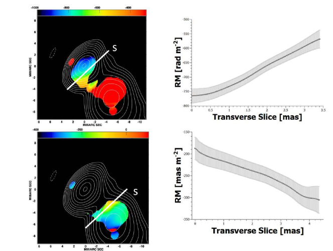
Figure 9: 4.6-GHz intensity map of 2037+511 with the RM distributions superposed. The contours shown are $-0.25$, 0.25, 0.50, 1, 2, 4, 8, 16, 32, 64 and 95% of the peak of 1.18 Jy/beam. The convolving beam is 3.2 mas $\times$ 1.9 mas in position angle $-40^{\circ}$. The colour scales for the upper and lower RM maps have been chosen to highlight the transverse gradients in the core and jet regions, respectively. The lines drawn across the RM distributions show the locations of the RM slices shown in the corresponding right-hand panels; the letter “S” at one end of these lines marks the side corresponding to the starting point for the slice.

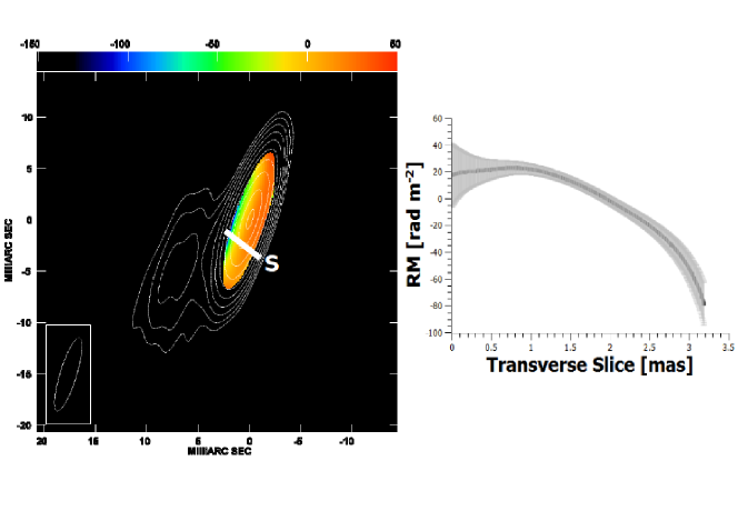
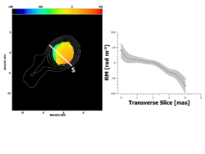
Figure 10: 4.6-GHz intensity map of 2345$-$167 with the RM distribution superposed, for convolution with the intrinsic elliptical beam (top left, 7.4 mas $\times$ 1.6 mas in position angle $-17^{\circ}$) and a circular beam with the same area (bottom left). The contours shown are $-0.25$, 0.25, 0.50, 1, 2, 4, 8, 16, 32, 64 and 95% of the peaks of 1.54 Jy/beam (top left) and 1.61 Jy/beam (bottom left). The lines drawn across the RM distributions show the locations of the RM slices shown in the corresponding right-hand panels; the letter “S” at one end of these lines marks the side corresponding to the starting point for the slice.

We were able to derive reasonable relative core shifts for this source, which were all quite small. The derived shifts relative to 15.4 GHz are given in Table 2.

Table 3: Detected transverse RM gradients
Source	Location	RM1	RM2	—$\Delta$RM—	Significance
		rad/m2	rad/m2	rad/m2
0333+321	Core	$-628\pm 35$	$-424\pm 28$	$204\pm 45$	$4.5\sigma$
	Jet	$-73\pm 35$	$+85\pm 12$	$158\pm 37$	$4.3\sigma$
0738+313	Core	$-553\pm 22$	$-957\pm 14$	$404\pm 27$	$15\sigma$
	Jet	$+34\pm 9$	$-70\pm 28$	$104\pm 30$	$3.5\sigma$
0836+710	Jet	$-191\pm 70$	$+125\pm 70$	$316\pm 100$	$3.2\sigma$
0923+392	Core	$-326\pm 70$	$+59\pm 70$	$386\pm 99$	$3.9\sigma$
	Jet	$-174\pm 69$	$-508\pm 69$	$334\pm 98$	$3.4\sigma$
1150+812	Jet	$+480\pm 45$	$+163\pm 37$	$317\pm 59$	$5.3\sigma$
1633+382	Core	$-78\pm 24$	$+140\pm 20$	$218\pm 32$	$6.8\sigma$
	Jet	$-103\pm 45$	$+41\pm 9$	$144\pm 46$	$3.1\sigma$
2037+511	Core	$-765\pm 24$	$-568\pm 25$	$197\pm 38$	$5.1\sigma$
	Jet	$-189\pm 30$	$-303\pm 24$	$114\pm 38$	$3.0\sigma$
2345$-$167 – Elliptical beam	Core	$-199\pm 38$	$+90\pm 31$	$289\pm 49$	$5.9\sigma$
2345$-$167 – Circular beam	Core	$-58\pm 18$	$+48\pm 21$	$106\pm 28$	$3.7\sigma$

Figure 9 presents the RM distribution for 2037+511 for our six frequencies, superimposed onto the 4.6 GHz intensity contours. We subtracted the effect of the integrated RM determined by Rusk (1988) from the observed polarization angles before making the RM map (Table 1); this led to only small adjustments in the observed polarization angles by no more than about $6^{\circ}$. The RM maps produced directly and taking into account the small relative shifts between the frequencies were very similar. Our RM map shows gradients transverse to the jet in both the core and inner jet, with opposite directions. Figure 9 shows two RM maps made with different RM ranges, to highlight the structure of the RM distribution in the core region (upper) and jet (lower). Figure 9 also shows two slices taken roughly perpendicular to the jet direction plotted together with their errors. The transverse RM gradients are monotonic, and have significances of approximately $5\sigma$ in the core region and $3\sigma$ in the jet.

3.8 2345$-$167

Figure 2d shows our 7.9 GHz polarization map for 2345$-$167. The core polarization is roughly orthogonal to the jet direction, suggesting a longitudinal magnetic field.

Due to the compactness of the source structure, it was not possible to determine reliable shifts between the maps at the different frequencies. Thus, our RM maps were derived without applying additional alignments to the input data.

The top panel of Figure 10 presents the RM distribution for 2345$-$167 for our six frequencies, superimposed onto the 4.6 GHz intensity contours. Because the integrated RM of Taylor et al. (2009) was very small, and would have led to completely negligible changes in the observed polarization angles, we did not subtract the effect of this integrated RM from the observed polarization angles for this source. A transverse RM gradient is visible across the region just southeast of the core. Figure 10 also shows a slice taken roughly perpendicular to the jet direction in this region, plotted together with its errors. The observed transverse RM gradient is monotonic, and has a significance of about $6\sigma$. Although the Monte Carlo simulations of Mahmud et al. (2013) and Murphy & Gabuzda (2013) have shown that reliable RM gradients can be detected even across very narrow structures, we tested the reality of this gradient by convolving with a circular beam with comparable area, with a full width at half maximum of 2.8 mas. The resulting RM map is shown in the lower panel of Fig. 10. The transverse RM gradient is still visible, and the slice shown indicates that it is monotonic. The statistical significance has been reduced by the convolution with a wider beam, but remains significant, at $3.5\sigma$.

4 Discussion

4.1 Reliability and Significance of the Transverse RM Gradients

Table 3 gives a summary of the transverse Faraday rotation measure gradients detected in the images presented here. The statistical significances of these gradients typically range from $3\sigma$ to $5\sigma$, with one value reaching nearly $15\sigma$. This indicates that none of the transverse RM gradients reported here are likely to be spurious (i.e., due to inadequacy of the $uv$ coverage and noise): the Monte Carlo simulations of Hovatta et al. (2012) and Murphy & Gabuzda (2013) have shown that spurious gradients at the $3\sigma$ level should arise for 4–6-frequency VLBA observations in the frequency interval considered here with a probability of no more than about 1%, with this probability being even lower for monotonic gradients encompassing differences of greater than $3\sigma$. Although the occurrence of spurious gradients rises substantially for VLBA observations of low-declination sources, the high significance of the gradient observed across the inner jet of 2345$-$167 with its intrinsic (elliptical) beam – about $6\sigma$ – is high enough to make it very improbable that this gradient is spurious.

In principle, it is optimal to ensure that the polarization angle maps are correctly aligned relative to each other using the measured VLBI core shifts before using them to construct RM maps. It was possible to find reliable core shifts for three of the AGNs considered here (0333+321, 0836+710, 2037+511); in three other cases, the core shifts were estimated to be negligible (0738+313, 0923+392, 1150+812); in the remaining two cases, it was not possible to get reliable core-shift estimates due to the compactness of the source structure (1633+382, 2345$-$167). The similarity of the RM maps made applying and not applying the relative shifts between the different frequencies in the three cases where this could be done gives us confidence that the RM maps for the three sources for which core shifts could not estimated are unlikely to be significantly affected by image misalignment.

The Monte Carlo simulations of Mahmud et al. (2013) and Murphy & Gabuzda (2013) have showed that it is not necessary or meaningful to place a limit on the width spanned by an RM gradient in order for it to be reliable, as long as the gradient is monotonic and the difference between the RM values at either end is at least $3\sigma$. We have used the single-pixel error estimates recommended by Hovatta et al. (2012) based on their own Monte Carlo simulations, to ensure that our single-pixel RM uncertainties are not underestimated.

Although the signal-to-noise ratio for our RM estimates could in principle be increased by averaging together some number of pixels surrounding a region of interest, the RM values being averaged would be highly correlated due to convolution with the CLEAN beam, making it very difficult to accurately estimate the corresponding uncertainty on the average value. For this reason, all the RM values we have considered are based on single-pixel estimates, for which the uncertainties are much better understood (Hovatta et al. 2012). Note that this is a conservative approach to estimating the statistical significances of the observed RM gradients.

4.2 Sign Changes in the Transverse RM Profiles

The observed Faraday rotation measure depends on both the density of thermal electrons and the line-of-sight magnetic field in the region where the Faraday rotation is occurring. Accordingly, gradients in Faraday rotation could reflect gradients in either the electron density or line-of-sight magnetic field (or both). However, if an observed gradient is monotonic and encompasses a change in the sign of the Faraday rotation, this cannot be explained by an electron-density gradient alone, and indicates a systematic change in the line-of-sight magnetic field, such as would come about in the case of a helical magnetic field geometry in the region of Faraday rotation.

Sign changes are observed in the transverse RM gradients detected in 0333+321, 0738+318, 0836+710, 0923+392, 1633+382 and 2345$-$167, strengthening the case that these gradients are due to helical magnetic fields associated with these jets.

Note that the absence of a sign change in the transverse RM profile does not rule out the possibility that a transverse gradient is due to a helical or toroidal field component in the region of Faraday rotation, since gradients encompassing only one sign can be observed for some combinations of helical pitch angle and viewing angle.

4.3 Core-Region Transverse RM Gradients

In the standard theoretical picture, the VLBI “core” represents the “photosphere” at the base of the jet, where the optical depth is roughly unity. However, in many cases, the observed core is likely a blend of this (partially) optically thick region and optically thin regions in the innermost jet. Since these optically thin regions are characterized by much higher degrees of polarization, they likely dominate the overall observed “core” polarization in many cases. Therefore, we have supposed that the polarization angles observed in the core are most likely orthogonal to the local magnetic field, as expected for predominantly optically thin regions. We have not observed any sudden jumps in polarization position angle by roughly $90^{\circ}$ suggesting the presence of optically thick–thin transitions in the cores in our frequency range at our epoch.

This picture of the observed VLBI core at centimeter wavelengths corresponding to a mixture of optically thick and thin regions, with the observed core polarization contributed predominantly by optically thin regions, also impacts our interpretation of the core-region Faraday rotation measures. Monotonic transverse RM gradients with significances of at least $3\sigma$ are observed across the core regions of 0333+321, 0738+318, 0923+392, 1150+812, 1633+382, 2037+511 and 2345$-$167. The simplest approach to interpreting these gradients is to treat them in the same way as transverse gradients observed outside the core region, in the jet. While the simulations of Broderick et al. (2010) show that relativistic and optical depth effects can sometimes give rise to non-monotonic transverse RM gradients in core regions containing helical magnetic fields, there are also cases when these helical fields give rise to monotonic RM gradients, as they would in a fully optically thin region. In addition, most of the non-monotonic behaviour that can arise will be smoothed by convolution with a typical centimeter-wavelength VLBA beam [see, for example, the lower right panel in Fig. 8 of Broderick et al. (2010)]. Therefore, when a smooth, monotonic, statistically significant transverse RM gradient is observed across the core region, it is reasonable to interpret this as evidence for helical/toroidal fields in this region (i.e., in the innermost jet).

4.4 RM-Gradient Reversals

We have detected distinct regions with transverse Faraday rotation gradients oriented in opposite directions in 0923+392 and 2037+511. Similar reversals in the directions of the RM gradients in the core region and inner jet have also been reported by Mahmud et al. (2013) for the AGNs 0716+714 and 1749+701.

This at first seems a puzzling result, since the direction of a transverse RM gradient associated with a helical magnetic field component is essentially determined by the direction of rotation of the central black hole and accretion disk and the initial direction of the poloidal field component that is “wound up” by the rotation. It is difficult in this simplest picture to imagine how the direction of the resulting azimuthal field component could change with distance along the jet or with time. However, in a picture with a nested helical field structure, similar to the “magnetic tower” model of Lynden–Bell (1996), but with the direction of the azimuthal field component being different in the inner and outer regions of helical field, such a change in the direction of the net observed RM gradient could be due to a change in dominance from the inner to the and outer region of helical field in terms of their overall contribution to the Faraday rotation (Mahmud et al. 2013). One theoretical picture that predicts a nested helical-field structure with oppositely directed azimuthal field components in the inner and outer regions of helical field is the “Poynting–Robertson cosmic battery” model of Contopoulos et al. (2009) [see also references therein], although other plausible systems of currents may also give rise to similar field configurations.

5 Conclusion

We have presented new polarization and Faraday RM measurements of eight AGNs based on 4.6–15.4 GHz observations with the Very Long Baseline Array. These objects were part of a sample of sources displaying evidence for polarization structures indicating a “spine” of transverse magnetic field flanked by a “sheath” of longitudinal magnetic field on one or both sides of the jet at one or more epochs in the 15.4-GHz MOJAVE images. One possible origin for this type of polarization structure is a helical jet magnetic field: depending on the pitch angle of the helical field and the viewing angle of the jet, the sky projection of the field may be predominantly orthogonal to the jet near the central ridge line, becoming predominantly longitudinal near the jet edges. If these jets do carry helical magnetic fields, their Faraday rotation measure (RM) distributions should also show a tendency to display transverse RM gradients, whose origin is the systematic change in the line-of-sight component of the helical field across the jet.

All eight of these AGNs show evidence for Faraday rotation measure (RM) gradients across their core regions and/or jets with statistical significances of at least $3\sigma$. Two more AGNs with spine–sheath polarization strucure observed in the same VLBA experiment showed no signs of such systematic transverse RM gradients. The fact that eight of ten AGNs displaying partial or full “spine–sheath” transverse polarization structures also show firm evidence for transverse RM gradients supports the hypothesis that both of these properties are due to the presence of a helical magnetic field associated with the VLBI jets of these AGNs. It is also striking that sign changes in the transverse RM profiles are observed for six of these eight AGNs, which can only be explained by a gradient in the line-of-sight magnetic field, not a gradient in electron density.

Two of the eight AGNs considered here — 0923+392 and 2037+511 — also show evidence for distinct regions with transverse Faraday rotation gradients oriented in opposite directions. This structure can also be seen in the RM map of 0923+392 presented by Zavala & Taylor (2003). Similar reversals in the directions of the RM gradients in the core region and inner jet have been reported by Mahmud et al. (2013) for the AGNs 0716+714 and 1749+701. This seemingly puzzling result can be explained in a picture with a nested helical field structure, with the direction of the azimuthal field component being different in the inner and outer regions of helical field. In this case, the reversal of the transverse RM gradient is due to a change in dominance from the inner to the and outer region of helical field in terms of their overall contribution to the Faraday rotation (Mahmud et al. 2013).

6 Acknowledgements

We thank Sebastian Knuettel for help in the preparation of this manuscript, Robert Zavala for providing the version of the AIPS task RM used for this work, and Gregory Tsarevsky for compiling his online catalog of integrated Faraday rotation measures, which was helpful in our analysis (http://lukash.asc.rssi.ru/people/Gregory.Tsarevsky/RM Cat96.html). We are also grateful to the anonymous referee for his or her quick response and thoughtful comments. This research has made use of data from the University of Michigan Radio Astronomy Observatory which has been supported by the University of Michigan and by a series of grants from the National Science Foundation, most recently AST-0607523.

References

- dummy (1893) Asada K., Inoue M., Nakamura M., Kameno S. & Nagai H. 2008, ApJ, 682, 798
- dummy (1893) Asada K., Nakamura M., Inoue M., Kameno S. & Nagai H. 2010, ApJ, 720, 41
- dummy (1893) Attridge J. M., Roberts D. H. & Wardle J. F. C. 1999, ApJ, 518, 87
- dummy (1893) Broderick A. E. & McKinney J. C. 2010, ApJ, 725, 750
- dummy (1893) Burn B.J. 1966, MNRAS, 133, 67
- dummy (1893) Contopoulos I., Christodoulou D. M., Kazanas D. & Gabuzda D. C. 2009, ApJ Letters, 702, 148
- dummy (1893) Gabuzda D. C., Cantwell T. M. & Cawthorne T. V. 2014, MNRAS, 438, L1
- dummy (1893) Hovatta T., Lister M. L., Aller M. F., Aller H. D., Homan D. C., Kovalev Y. Y., Pushkarev A. B. & Savolainen T. 2012, AJ, 144, 105
- dummy (1893) Hovatta T., Aller M. F., Aller H. D., Clausen–Brown E., Homan D. C., Kovalev Y. Y., Lister M. L., Pushkarev A. B. & Savolainen T. 2014, AJ, 147, 143
- dummy (1893) Lister M. L. & Homan D. C. 2005, AJ, 130, 1389
- dummy (1893) Lovelace R. V. E., Li H., Koldoba A. V., Ustyugova G. V. & Romanova M. M. 2002, ApJ, 572, 445
- dummy (1893) Lynden–Bell D. 1996, MNRAS, 279, 389
- dummy (1893) Lyutikov M., Pariev V. & Gabuzda D. C. 2005, MNRAS, 360, 869
- dummy (1893) Mahmud M., Gabuzda D. C. & Bezrukovs V. 2009, MNRAS, 400, 2
- dummy (1893) Mahmud M., Coughlan C. P., Murphy E., Gabuzda D. C. & Hallahan R. 2013, MNRAS, 431, 695
-
dummy (1893)
Murphy E. & Gabuzda D. C. 2013, in The Innermost Regions
of Relativistic Jets and Their Magnetic Fields, EPJ Web of Conferences,
Volume 61, id.07005 (http://www.epj-conferences.org/articles/epjconf/abs/2013/22/
epjconf_rj2013_07005/epjconf_rj2013_07005.html) - dummy (1893) Nakamura M., Uchida Y. & Hirose S. 2001, New Astronomy, 6, 2, 61
- dummy (1893) Pacholczyk A. G., 1970, Radio Astrophysics, W. H. Freeeman , San Franciso
- dummy (1893) Pushkarev A. B., Gabuzda D. C., Vetukhnovskaya Yu. N. & Yakimov V. E. 2005, MNRAS, 356, 859
- dummy (1893) Pushkarev A. B., Hovatta T., Kovalev Y. Y., Lister M. L., Lobanov A. P., Savolainen T. & Zensus J. A. 2012, A&A, 545, 113
- dummy (1893) Rudnick L. & Jones T. W. 1983, AJ, 88, 518
- dummy (1893) Rusk R. E. 1988, PhD Thesis, University of Toronto
- dummy (1893) Simard–Normandin M., Kronberg P. P. & Button S. 1981, ApJ Supplement Series, 45, 91
- dummy (1893) Taylor A. R., Stil J. M. & Sunstrum C. 2009, ApJ, 702, 1230
- dummy (1893) Zavala R. T. & Taylor G. B. 2003, ApJ, 589, 126