Zero Mode Tunnelling in a Fractional Quantum Hall Device

Abstract

Tunnelling measurements on fractional quantum Hall systems are continuing to increase in popularity since they provide a method to probe the non-Fermi liquid behaviour of fractionally charged excitations occupying the edge states of a quantum Hall system. When considering tunnelling one must resort to an effective theory and typically a phenomenological tunnelling Hamiltonian is used analogous to that used for a conventional Luttinger liquid. It is the form of this tunnelling Hamiltonian that is investigated in this work by making a comparison to an exact microscopic calculation of the zero mode tunnelling matrix elements. The computation is performed using Monte Carlo and results were obtained for various system sizes for the $\nu=1/3$ Laughlin state. Here we also present a solution to overcome the phase problem experienced in Monte Carlo calculations using Laughlin-type wavefunctions. Comparing the system size dependence of the microscopic and phenomenological calculations for the tunnelling matrix elements, it was found that only for a particular type of operator ordering in the tunnelling Hamiltonian was it possible to make a good match to the numerical calculations. From the Monte Carlo data it is also clear that for any system size the electron tunnelling is always less relevant than the quasiparticle tunnelling process, supporting the idea that when considering tunnelling at a weak barrier, the electron tunnelling process can be neglected.

One of the key signatures of the fractional quantum Hall effect (FQHE) are plateaus in the Hall conductance which are given by some rational factor, $\nu$ multiplied by the ratio $e^{2}/h$ Tsui et al. (1982). It is well understood that the bulk states of the system are incompressible Laughlin (1983) and thus transport properties are completely determined by 1D channels occupying the edges of the FQH droplet. These 1D channels consist of interacting electrons for which the Fermi liquid theory breaks down and it was first proposed by Wen Wen (1990) that they should instead, be described by a chiral Luttinger liquid. A chiral Luttinger liquid has the key feature of low-energy excitations being collective sound modes and it can be shown that the system has a four-terminal Hall conductance given by $\nu(e^{2}/h)$ Wen (1990). These features are similar to a conventional Luttinger liquid in which there are left and right moving particles along the same one dimensional channel. The chiral Luttinger liquid is a phenomenological theory useful for describing transport properties of the FQHE which are readily accessible to experimental measurements.

More recently, a great amount of theoretical and experimental effort has focused on the transport properties of FQH edge states when the charge carriers are faced with a single, or multiple potential barriers and tunnelling is observed. There are two equivalent methods to initiate tunnelling in a QH device. The most common from an experimentalists point of view is by physically moving the edges closer together at some point along a Hall bar, known as a quantum point contact (QPC). Such a constriction can be achieved by placing metallic plates above the 2D electron gas and applying a negative bias causing a local depletion of electrons. As a result edge states are brought closer together causing a finite probability of inter edge back scattering. The strength of this pinching effect on the edge states is determined by the magnitude of the bias applied to the magnetic plates. For ideal systems, the same tunnelling behaviour can be obtained from placing an impurity into the bulk which also couples the edges and allows back scattering to occur. Realistically using an impurity is a much cleaner method to observe basckscattering since a QPC can have adverse effects on the surrounding quantum Hall fluid due to electrostatic reconstruction as discussed in the review by Chang Chang (2003).

One of the first pieces of work concerned with tunnelling at a QPC was carried out by Kane and Fisher Kane and Fisher (1992a, b, c) who investigated tunnelling at both a weak link and a weak barrier in a conventional Luttinger liquid. Similar work was also carried out by Furusaki and Nagaosa Furusaki and Nagaosa (1993) and Moon et al. Moon et al. (1993). At a weak link tunnelling will be dominated by electrons in the Luttinger liquid since, effectively the liquid is split into two separate islands. For a weak barrier however it is the excitations of the Luttinger liquid that tunnel. For the work carried out by Kane and Fisher a perturbative approach for the tunnelling Hamiltonian was used in conjunction with RG to discover which of the tunnelling processes were relevant in both the strong and weak back scattering limit and predictions were made about the tunnelling conductance and the zero-bias peaks in I-V characteristics. The predictions about the Luttinger liquid behaviour show stark contrasts to that of the non-interacting system, the Fermi liquid. Here, unlike in the non-interacting case, the width of the zero-bias peaks are temperature dependent, and in particular the conductance away from the peak has a power law temperature dependence where the exponent of the power law is the interaction parameter of the Luttinger liquid. The reason for the differences is of course down to the interactions between the Fermions in 1D and thus observing such behaviour in a 1D channel will be key in discovering systems that are strongly correlated, non-Fermi liquids. The form of the tunnelling Hamiltonian used in all of the referenced works in this report can be mapped onto the boundary sine-Gordon model Gogolin et al. (2004) and consists of operators that annihilate a charge carrier in one direction and create another carrier traveling in the opposite direction at some barrier.

So far there is experimental agreement of non-Fermi liquid behaviour in the Laughlin type edge states of a FQH device Milliken et al. (1996); Roddaro et al. (2004) though the specific value of the power of the temperature dependence of the tunnelling conductance is slightly off the expected theoretical value Chang et al. (1996). Experiments measuring shot noise and interference experiments (all making use of one or multiple point contacts) are predicted to prove the existence of fractionally charged carriers in the edge states as well as display their (Abelian or non-Abelian) fractional statistics. In particular it has been predicted that for Laughlin type QH states, the back scattered current in shot noise experiments should be proportional to the charge of the carriers Kane and Fisher (1994) given by $e^{*}=\nu e$ in the weak back scattering limit at zero temperature, where $\nu$ is the filling fraction of the lowest Landau level. Experimental work has claimed to have observed Laughlin type quasiparticles in such experiments Saminadayar et al. (1997); dePicciotto et al. (1997) though not all of the work agrees that the shot noise measurement is dependent only on the charge of the quasiparticles. It has been claimed that the specifics of the tunnelling barrier as well as the energy regimes used in the experiment can effect the value of the back scattered current, this would account for a deviance in the predicted value of the quasiparticle charge in the very weak back scattering limit obtained in some experiments Dolev et al. (2010). In particular, the boundary sine-Gordon model for various test states has not been able to resolve which ground state provides a good description for even denominator filling fractions such as $\nu=5/2$. Experiments at quantum point contacts for the $\nu=5/2$ states which measure tunnelling noise and tunnelling conductance give predictions for quasiparticle charge $e^{*}$ and the tunnelling particles interaction parameter Baer et al. (2014), $g$. There is still no obvious match to the theoretical predictions of the various candidate states for the edges in the $\nu=5/2$ system Yang and Feldman (2013) and even distinguishing whether the state should display Abelian or non-Abelian statistics is not obvious.

The RG approach by Kane and Fisher is based on a 1D lattice model and it is assumed that the edge states of the FQHE will display similar behaviour so this approach is frequently used as a base model for theoretical predictions on transport properties of the FQHE. There are important differences between the Luttinger liquid model used for the perturbative RG analysis by Kane and Fisher and the FQH edge states. The electron field operators in the Luttinger liquid model can be derived microscopically from the 1D Hamiltonian describing a system of interacting electrons. It is not the same for the FQH edge states since in this case, the edge states result from a two-dimensional system of electrons in a strong magnetic field, thus the low-energy effective theory is obtained by projecting the FQH states onto the space of low energy edge states. The perturbative RG approach that works so well for the lattice model Luttinger liquid cannot be extended straightforwardly to the FQH edge states since it relies on the fact that interactions between electrons can be treated perturbatively. Switching off the electron-electron interactions in the FQHE destroys the effects existence. So how do these differences affect the formulation of a chiral Luttinger liquid as compared to that of a conventional Luttinger liquid?

It is already understood that the low energy projection of the edge states in the FQHE do not display exactly the same behaviour as the Luttinger liquid. One example is the low energy projection of the electron field operator. In the Luttinger liquid the anti-commutation relation for two spatially separated electron fields is given by a delta function, the same behaviour of similar fields in the edges states of a FQH system is not observed. There is another issue with the locality of the effective tunnelling Hamiltonian for a quasiparticle being transferred between two disconnected edges in the system. In the FQHE the tunnelling Hamiltonian takes a similar form to that of the tunnelling Hamiltonian in the conventional Luttinger liquid. I.e. the operator consists of creating a particle in one of the QH edge states and annihilating a particle in the opposing edge Moon et al. (1993); Fendley et al. (1995). Without the perturbative RG analysis at our disposal for FQH states there is no guarantee that the effective theory tunnelling operators will be local. For the Luttinger liquid model however, local operators in the microscopic theory are guaranteed to remain local in the effective theory using the Kadanoff coarse graining procedure.

The problem of the locality of the tunnelling Hamiltonian has been investigated and for a FQH system containing multiple quantum point contacts. It was observed that the tunnelling operators at one of the QPC’s did not commute with the tunnelling operator at a different QPC, independent on the magnitude of their spatial separation Guyon et al. (2002). To impose the expected locality which the quasiparticle tunnelling operators should adhere, the effective quasiparticle operators had additional Klein factors included in their representation Guyon et al. (2002); Kane (2003); Safi et al. (2001); Law et al. (2006); Vishveshwara (2003); Nayak et al. (1999); Ponomarenko and Averin (2004). The addition of the Klein factors adds an extra phase to the quasiparticle fields and it is reasoned that this is a statistical phase which is gained during a tunnelling event between two disconnected edges. This statistical phase is a result of the fractional statistics obeyed by the quasiparticles. Including Klein factors results in the effective quasiparticle tunnelling operators at two different QPC to commute with one another. Results on observables such as tunnelling currents are greatly dependent on the inclusion of these Klein factors (for example compare work by Law et al. Law et al. (2006) with Jonckheere et al. Jonckheere et al. (2005)).

In this work the low-energy projection of the tunnelling Hamiltonian is investigated for the quantum Hall edge states by making comparisons to microscopic calculations. In particular the form of the tunnelling Hamiltonian is tested for a quasiparticle and an electron in the $\nu=1/3$ FQH state by comparing it to exact microscopic calculations for the zero modes of the edge states. From the perturbative RG analysis on the conventional Luttinger liquid model, for a sufficiently weak barrier at $\nu=1/3$, the only relevant tunnelling should be that of single Laughlin quasiparticle with charge $e^{*}=\nu e$. Electron, and any combination of multiple quasiparticle tunnelling should be suppressed in the weak back scattering regime. Without any initial conditions to impose from a microscopic theory it is not obvious at exactly what energy scales in the FQHE that these higher-order tunnelling terms become irrelevant. From microscopic calculations presented here however, it can be deduced at what (if at all) system sizes the electron and quasiparticle tunnelling amplitudes become comparable. The microscopic calculation for the tunnelling of particles is carried out numerically using Monte Carlo where we focus on the simple case of investigating how an impurity, when placed between two disconnected edges in the bulk, affects the groundstate system. The effective theory tunnelling model already makes strong predictions about the way these zero mode matrix elements should behave for increasing system size and it is this relationship in particular that is tested. We find that the microscopic computations are in good agreement with the model so long as a specific type or ordering of operators is used in the tunnelling Hamiltonian. If one chooses to use normal ordered operators, which of course is convenient, then a normalisation factor dependent on the system size should be included. Such a normalisation factor would also make the tunnelling operator local.

The layout of this report is as follows; in section I. the geometry of the FQH system is introduced and the specifics of the chiral Luttinger liquid formalism is reviewed. The predictions of the sine-Gordon model for the specific geometry considered in this work are also calculated. Section II. discusses the Monte Carlo (MC) calculations whilst in the final section the MC results are presented and comparisons are made to the effective low energy model of the tunnelling operators.

1 Overview of the Chiral Luttinger Liquid and the Boundary Sine-Gordon Model Predictions

In this work, only FQH states occupying the lowest Landau level are considered. Since the exact ground state of a FQH system is not known, we instead use the Laughlin wavefunction which has been shown to be a good approximation for the system. This wavefunction is an exact solution for an Hamiltonian in terms of Haldane’s pseudo-potentials Haldane (1983). For a droplet of $N$ electrons in the lowest Landau level with filling factor $\nu=m^{-1}$, where $m$ is an odd integer, Laughlin’s wavefunction Laughlin (1983) has the form

$$\Psi_{N}=\displaystyle\prod_{k=1}^{N}{\left(e^{-\frac{|z_{k}|^{2}}{4l}}\right)}\prod_{i<j}^{N}{(z_{i}-z_{j})^{m}}$$ (1)

where $l$ is the magnetic length which, for the remainder of this work will be set to unity. The $\{z_{i}\}$ correspond to electron positions and the FQH droplet has a radius $R=\sqrt{2mN}$. It is noted that this wavefunction is not normalised. To create a second edge in our system such that tunnelling across the bulk can be observed, a macroscopic hole is inserted in the centre of the droplet. This macroscopic hole is created by inserting $M$ quasiholes at $z=0$. Mathematically, this corresponds to an extra product over particle coordinates in the wave function.

$$\Psi_{N}^{M}=\prod_{k=1}^{N}{\left(e^{-\frac{|z_{k}|^{2}}{4l}}z_{k}^{M}\right)}\prod_{i<j}^{N}{(z_{i}-z_{j})^{m}}\equiv\left|N,M\right\rangle$$ (2)

The bra-ket notation has been introduced to simplify expressions in future calculations. A schematic diagram of the device is shown in Figure 1. Now the electrons are confined to a domain $D^{M}$ on the complex plane. The hole created at $z=0$ has a radius $R_{I}=\sqrt{2M}$ and the outer radius is given by $R_{O}=\sqrt{2mN+2M}$. At the inferaces of $D^{M}$ there is a sharp decrease of particle density to zero in the large $N$ limit.

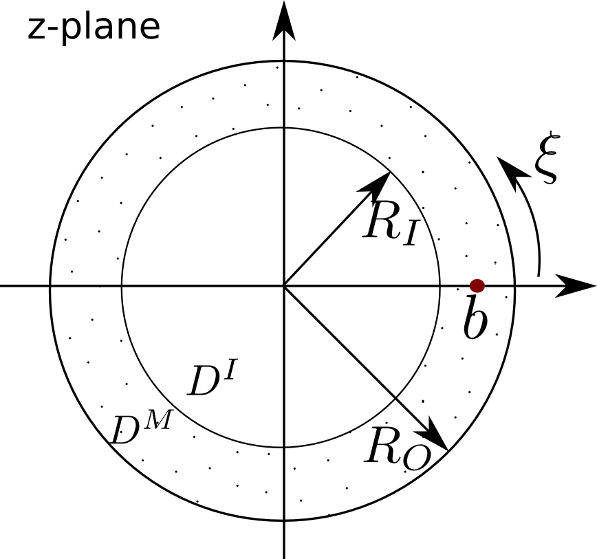
Figure 1: Schematic diagram for the FQH device. Charges are confined to the domain $D^{M}$ on the complex plane. The radii of the inner and outer edge of $D^{M}$ are given by $R_{I}$ and $R_{O}$. The width of domain $D^{M}$ is such that $R_{O}-R_{I}\sim 4$. Domain $D^{I}$ corresponds to the area of the macroscopic hole created by inserting Laughlin quasiholes at $z=0$. An impurity is placed at position $b$ along the positive real axis.

To encourage tunnelling between the edges of the system, an impurity is placed inside the bulk at position $b$. The potential $\hat{V}$ of this impurity has the form

$$\hat{V}=u\sum_{i=1}^{N}\delta^{(2)}(z_{i}-b).$$ (3)

The parameter $u$ corresponds to the strength of the potential which will be set to unity and we assume that $|b|=(R_{O}+R_{I})/2$. If the ring of the bulk is sufficiently thick then adding the impurity to the system will have no effect on the edges due to a finite correlation length in the bulk on the order of the magnetic length. Therefore it is assumed that for all $N$ the width of the system ($R_{O}-R_{I}$) is constant and narrow enough such that both edges are affected by the impurity.

As implied in the introduction, it is the edges of the device, consisting of two counter propagating chiral Luttinger liquids that are of most interest for this work. A successful method of the describing the effective low-energy physics of a Luttinger liquid uses the method of bosonization. There are various approaches to deriving the electron fields and in this report a similar notation is used to the formalism in A. Boyarsky (2004) and Ivan P. Levkivskyi (2010). Here, operators are projected onto the subspace of edge excitations which defines the zero mode operators and Boson creation and annihilation operators for quasiparticles. It is assumed that the edges are sufficiently far apart that they do not interact away from the impurity and thus each edge has its own electron field operators.

In the effective theory of low-energy excitations the transverse positions to the edges of the FQH device are unimportant since we assume that the domain $D^{M}$ is a very narrow ring in comparison to the size of its outer radius $R_{O}$, therefore our particle fields depend only on the longitudinal coordinate $\xi$, where $\xi\in[0,2\pi R]$ and $R$ is the radius at which the transfer of charges between the edges takes place, i.e. $R\equiv|b|$. One can write the bosonization formulae for general field operators $\psi_{p}$ in the low-energy effective theory, where $p$ is some integer and $\psi_{p}$ corresponds to the annihilation operator of particle with charge $e^{*}=(p/m)e$ in the Laughlin state $\nu=(1/m)$. Therefore $\psi_{p=1}$ corresponds to the field for a single Laughlin quasiparticle with charge $e^{*}=(1/m)e$ and $\psi_{p=m}$ corresponds to $m$ quasiparticles, or equivalently a single electron field.

$$\psi^{\dagger}_{p,O}(\xi) = e^{i\frac{p}{m}\varphi_{N}}e^{p\phi_{O}(\xi)}$$

$$\psi_{p,O}(\xi) = e^{-p\phi_{O}(\xi)}e^{-i\frac{p}{m}\varphi_{N}}$$

$$\psi^{\dagger}_{p,I}(\xi) = e^{i\frac{p}{m}\varphi_{N}}e^{ip\varphi_{M}}e^{p\phi_{I}(\xi)}$$

$$\psi_{p,I}(\xi) = e^{-p\phi_{I}(\xi)}e^{-i\frac{p}{m}\varphi_{N}}e^{-ip\varphi_{M}}$$ (4)

The subscript ”I” corresponds to an inner boundary operator and ”O” to an outer boundary operator. The fields $\phi_{O/I}$ are bosonic and are given by

$$\phi_{O}(\xi) = -\frac{i\xi}{R}(\theta_{N}+\frac{\theta_{M}}{m})+\sum_{k>0}\sqrt{\frac{1}{mk}}\left(e^{-ik\frac{\xi}{R}}a_{k}^{\dagger}-e^{ik\frac{\xi}{R}}a_{k}\right)$$

$$= \phi_{O}^{0}+\phi_{O}^{+}-\phi_{O}^{-}$$

$$\phi_{I}(\xi) = -\frac{i\xi}{mR}\theta_{M}+\sum_{k>0}\sqrt{\frac{1}{mk}}\left(e^{ik\frac{\xi}{R}}a_{-k}^{\dagger}-e^{-ik\frac{\xi}{R}}a_{-k}\right)$$ (5)

$$= \phi_{I}^{0}+\phi_{I}^{+}-\phi_{I}^{-}.$$

The short hand notation of decomposing the the field $\phi$ into zero mode parts ($\phi^{0}$), creation operator parts ($\phi^{+}$) and annihilation operator parts ($\phi^{-}$) will be used in subsequent calculations. The $a^{\dagger}_{\pm k}$ and $a_{\pm k}$ are edge excitation creation and annihilation operators for a given excitation orbital $k$ which may correspond to either the outer (”+”) or inner (”-”) boundary. Operators $\theta_{N/M}$ and $e^{i\varphi_{N/M}}$ are conjugate zero mode operators and act as follows;

$$e^{i\varphi_{N}}\left|N,M\right\rangle = \left|N+1,M\right\rangle$$

$$\theta_{N}\left|N,M\right\rangle = N\left|N,M\right\rangle$$

$$e^{i\varphi_{M}}\left|N,M\right\rangle = \left|N,M+1\right\rangle$$

$$\theta_{M}\left|N,M\right\rangle = M\left|N,M\right\rangle$$

where $\left|N,M\right\rangle$ is the Laughlin groundstate for a system of $N$ electrons and $M$ quasiholes. In this effective theory the states $\left|N,M\right\rangle$ are normalised and orthogonal such that $\left\langle N,M|N^{\prime},M^{\prime}\right\rangle=\delta_{N,N^{\prime}}\delta_{M,M^{\prime}}$ in the large $N$ limit Laughlin (1983). The operators for the outer and inner boundary are independent and thus all commute with one another. In summary, a list of useful commutation relations are;

$$\left[\theta_{x},e^{i\varphi_{y}}\right] = e^{i\varphi_{x}}\delta_{x,y}\quad\textrm{where}\quad x\,\,\textrm{or}\,\,y=N\,\,\textrm{or}\,\,M$$

$$\left[a_{\pm p},a^{\dagger}_{\pm k}\right] = \delta_{p,k}$$

$$\left[a_{\pm p},a^{\dagger}_{\mp k}\right] = 0$$ (6)

With the low-energy, effective theory field operators defined, one can now discuss the effect of the impurity placed in the bulk. The form of the tunnelling operator used in all the referenced work in the introduction takes the form

$$H_{T}=\sum_{p=1}^{\infty}A_{p}(\xi)$$ (7)

where $\xi$ is the longitudinal position at which tunnelling occurs along the boundaries and operators $A_{p}$ transfer a number of $p$ quasiparticles from the inner to the outer boundary. From the form of $H_{T}$ one can see it is possible for the tunnelling of any number of quasiparticles across the bulk. For $p=1$, $A_{P}$ describes the tunnelling process for a single quasiparticle and for $p=m$ the tunnelling process is for that of an electron in FQH state $\nu=1/m$. For Laughlin states however, it can be seen from a microscopic calculation (see section II. for details) that the transfer of $p>m$ quasiparticles is identically zero. Whether this behaviour should be extended to the exact wavefunctions of quantum Hall states is doubtful and thus experiments on FQH systems that measure a $p>m$ tunnelling process would be extremely interesting and a good measure for the preciseness of Laughlin’s wavefunction as a description FQHE.

Here two types of tunnelling processes across the bulk are considered, the first being a single quasiparticle tunnelling and the second will be electron tunnelling or equivalently $m$ quasiparticles tunnelling. These processes are described by $A_{p=1}$ and $A_{p=m}$ respectively. In general operators $A_{p}$ have the form;

$$A_{p}(\xi)=t_{p}\left(\psi_{p,O}^{\dagger}(\xi)\psi_{p,I}(\xi)+\textrm{h.c.}\right).$$ (8)

where $\xi$ is the longitudinal position at which the tunnelling occurs on the boundaries and $t_{p}$ is a parameter that cannot be calculated analytically given the microscopic theory. In this work the scaling behaviour of the parameters $t_{p}$ will be investigated as system size $N$ is varied. This can be achieved by looking at the zero mode matrix elements of the tunnelling elements.

$$\left\langle A_{p}(\xi)\right\rangle = \left\langle N,M\right|A_{p}(\xi)\left|N^{\prime},M^{\prime}\right\rangle$$ (9)

$$= t_{p}\left\langle N,M\right|\psi_{p,O}^{\dagger}(\xi)\psi_{p,I}(\xi)\left|N^{\prime},M^{\prime}\right\rangle+\textrm{h.c.}$$

$$= t_{p}\left\langle N,M\right|e^{i\frac{p}{m}\varphi_{N}}e^{p\phi_{O}(\xi)}e^{-p\phi_{I}(\xi)}e^{-i\frac{p}{m}\varphi_{N}}e^{-ip\varphi_{M}}\left|N^{\prime},M^{\prime}\right\rangle+\textrm{h.c.}$$

The first term in (9) describes a process where $p$ particles move from the inner boundary to the outer boundary and for the second term this process is reversed. Only one term is needed here so the Hermitian conjugate term can be neglected. Next the ordering of the operators is considered which will in turn affect the behaviour of the parameter $t_{p}$. Here, two types of ordering are considered with the first being the usual definition of normal ordering defined by

$$e^{\phi}\rightarrow:e^{\phi}:\,=e^{\phi^{0}}e^{\phi^{+}}e^{-\phi^{-}}$$ (10)

The matrix element calculated using this ordering is denoted by $\left\langle:A_{p}(\xi):\right\rangle$ and is straightforward to calculate.

$$\left|\left\langle:A_{p}(\xi):\right\rangle\right|=\left|\left\langle N,M\left|e^{i\frac{p}{m}\varphi_{N}}:e^{p\phi_{O}(\xi)}::e^{-p\phi_{I}(\xi)}:e^{-i\frac{p}{m}\varphi_{N}}e^{-ip\varphi_{M}}\right|N^{\prime},M^{\prime}\right\rangle\right|=|t_{p}|\delta_{N,N^{\prime}}\delta_{M,M^{\prime}-p}$$ (11)

Note that the absolute values of matrix elements are taken to get rid of unnecessary phase terms. Therefore if normal ordering is used, only $t_{p}$ contributes to system size dependence. On the other hand, a different result is obtained by choosing the following ordering for the operators,

$$e^{\phi}\,=e^{\phi^{0}}e^{\phi^{+}}e^{-\phi^{-}}e^{-\frac{1}{2}[\phi^{0},\phi^{+}-\phi^{-}]}e^{-\frac{1}{2}[\phi^{+},-\phi^{-}]}=e^{\phi^{0}}e^{\phi^{+}}e^{-\phi^{-}}e^{-\frac{1}{2}\sum_{k}(\frac{m}{k})}$$ (12)

where the following commutation relations have been used; $[\phi^{0}_{x}(\xi),\phi^{+}_{x}(\xi)-\phi^{-}_{x}(\xi)]=0$ and $[\phi^{+}_{x}(\xi),\phi^{-}_{x}(\xi)]=-\sum_{k}(m/k)$ where $x=I$ or, $x=O$. These relations are straightforward to calculate using the correlators listed in (1). Proceeding with the matrix element (9);

$$\left|\left\langle A_{p}(\xi)\right\rangle\right| = |t_{p}|\exp\left(-\sum_{k>0}\frac{p^{2}}{mk}\right)\left|\left\langle N-1,M\right|e^{p\phi_{O}^{0}}e^{p\phi_{O}^{+}}e^{-p\phi_{O}^{-}}e^{-p\phi_{I}^{0}}e^{-p\phi_{I}^{+}}e^{p\phi_{I}^{-}}\left|N^{\prime}-1,M^{\prime}-m\right\rangle\right|$$ (13)

$$= |t_{p}|\exp\left(-\sum_{k>0}\frac{p^{2}}{mk}\right)\delta_{N,N^{\prime}}\delta_{M,M^{\prime}-p}$$

The final step is to carry out the sum over $k$ in (13). There are two natural cutoffs that can be considered for the low-energy limit of the system. The first is related to the breakdown of the Boson creation and annihilation operators in the Luttinger liquid theory which are only independent operators for $k\leq N$. Therefore $N$ could be a valid cutoff for the sum. However there is also an obvious limit on the energy of the edge excitations which is related to the bulk energy gap. If quasiparticles have an energy larger than the bulk gap energy $\Delta$ then they are able to travel through the bulk destroying the physics of the Luttinger liquid edge states in the FQHE. The dispersion relation for the Bose excitations is linear at the edge and so the maximum momentum for a quasiparticle is $p=\Delta/v$ where $v$ is the quasiparticle velocity. The momentum corresponding to a given edge orbital $k$ is also given by $p=\hbar k/R$ and therefore the maximum value of the orbital according to the bulk energy gap is $k\leq R\Delta/(v\hbar)\equiv\Lambda$. Recall that $R\equiv|b|$, the point at which tunnelling occurs, and taking into account the constraint on $M$ that for any $N$ one must always have $R_{O}-R_{I}\sim 4$, then the magnitude of the impurity, $b$ is on the order of $N$ in the large $N$ limit. Thus the two cutoffs are essentially equivalent. In this work we use $\Lambda\sim R\equiv|b|$ as the cutoff, which has more of an apparent, physical meaning.

The sum over $k$ in (13) is performed using $\Lambda\sim R\equiv|b|$ as a soft cutoff such that $\sum_{k>0}k^{-1}\rightarrow\sum_{k>0}k^{-1}e^{-k/R}=-\ln(1-e^{-1/R})$. To get an approximate idea of the behaviour of this sum in the large $N$, or equivalently large $R$ limit, the exponential in the logarithm can be expanded to give $-\ln(1-e^{-1/R})\sim\ln R$. Thus for a log-log plot of the amplitude of (13) versus particle number, one would expect the gradient to be $\sim-p^{2}/m$ for large enough $R\equiv|b|$. For now we will keep the exact form of the sum so that the final expression of the tunnelling matrix elements is,

$$\left|\left\langle A_{p}(\xi)\right\rangle\right|=|t_{p}|\left(1-e^{-\frac{1}{R}}\right)^{\frac{p^{2}}{m}}\delta_{N,N^{\prime}}\delta_{M,M^{\prime}-p}$$ (14)

From (14); the zero mode tunnelling matrix elements have a dependence on the system size $N$, which for non-normal ordering given by (12) is not from the parameter $t_{p}$. If $A_{p}$ for ordering (12) is local then we can assume all the system size dependence originates from the sum $\sum_{k}k^{-1}$ and $t_{p}$ is constant for all $N$. Ideally the tunnelling operators should remain local since the impurity placed between the edges in the FQH device should only affect carriers in its vicinity and not the remainder of the system. The correlator of a local operator $\left\langle A_{p}(\xi)A_{p}(\xi^{\prime})\right\rangle$ should be independent of system size for $\xi$ and $\xi^{\prime}$ sufficiently far apart, also $\xi$, $\xi^{\prime}$ should be sufficiently far away from the edges of the system.

$$\left\langle A_{p}(\xi)A_{p}(\xi^{\prime})\right\rangle = \left\langle N,M\right|A_{p}(\xi)A_{p}(\xi^{\prime})\left|N^{\prime},M^{\prime}\right\rangle$$ (15)

$$= 2\exp\left\{\frac{2p^{2}}{m}\sum_{k>0}k^{-1}\left(\cos\left[\frac{k}{R}(\xi^{\prime}-\xi)\right]-1\right)\right\}\cos\left[\frac{p}{R}\left(N-\frac{p}{m}\right)(\xi^{\prime}-\xi)\right]$$

Only matrix elements that are kept in the above expression are those with $M^{\prime}=M$ and $N^{\prime}=N$ which satisfies the definition of the tunnelling operator $A_{p}$.

To finish the calculation, a soft cutoff is used ($\Lambda\equiv R$) to calculate the sum in (15) which is the same approach as was used to calculate similar sums earlier for the tunnelling matrix elements. Using this cutoff and taking the limit $|\xi-\xi^{\prime}|/R<<1$ gives the final result for the correlator calculation which has, as required, no system size independence.

$$\left\langle A_{p}(\xi)A_{p}(\xi^{\prime})\right\rangle=\frac{2}{\left(1+(\xi^{\prime}-\xi)^{2}\right)^{\frac{p^{2}}{m}}}\cos\left[\frac{p}{R}\left(N-\frac{p}{m}\right)(\xi^{\prime}-\xi)\right]$$ (16)

The correlator of the tunnelling operator for normal ordering, $\left\langle:A_{p}(\xi)::A_{p}(\xi^{\prime}):\right\rangle$ does have system size dependence and therefore tunnelling operators $A_{p}$ defined by ordering (12) are preferred. To summarise this section; expressions for the zero mode matrix tunnelling elements have been calculated for both normal ordered operators (11) and for non-normal ordered operators (14). In the normal ordered case there is system size dependence which must be encoded in the parameter $t_{p}$. For the non-normal ordered tunnelling operators, this size dependence comes from the calculation of the matrix elements and the operator algebra itself. Since the non-normal ordered tunnelling matrix elements show explicit size dependence and were obtained from local tunnelling operators, we concentrate on these when making comparisons with the microscopic theory discussed in the next section.

2 Microscopic Calculations for Tunnelling Matrix Elements

The results for the effective theory tunnelling operators calculated in the previous section should also manifest from a microscopic theory. Here it is assumed that the Laughlin state is exact wavefunction for the FQH system with filling factor $\nu=1/m$, where $m$ is odd. The microscopic expression for the zero mode tunnelling matrix elements are given by

$$\left\langle V\right\rangle_{\chi} \equiv \frac{\left\langle N,M\left|V\right|N,M+\chi\right\rangle}{\sqrt{\left\langle N,M|N,M\right\rangle\left\langle N,M+\chi|N,M+\chi\right\rangle}}$$ (17)

$$= \frac{\displaystyle\int\prod_{k=1}^{N}\left(\textrm{d}^{2}z_{k}\,e^{-\frac{|z_{k}|^{2}}{2}}|z_{k}|^{2M}z_{k}^{\chi}\right)\prod_{i<j}^{N}|z_{i}-z_{j}|^{2m}\sum_{n=1}^{N}\delta^{(2)}(z_{n}-b)}{\displaystyle\left[\int\prod_{k=1}^{N}\left(\textrm{d}^{2}z_{k}\,e^{-\frac{|z_{k}|^{2}}{2}}|z_{k}|^{2M}\right)\prod_{i<j}^{N}|z_{i}-z_{j}|^{2m}\cdot\int\prod_{k=1}^{N}\left(\textrm{d}^{2}z_{k}\,e^{-\frac{|z_{k}|^{2}}{2}}|z_{k}|^{2(M+\chi)}\right)\prod_{i<j}^{N}|z_{i}-z_{j}|^{2m}\right]^{\frac{1}{2}}}$$

This matrix element describes a process in which a number of $\chi$ quasiparticles is transferred from the inner boundary to the outer boundary due to the impurity potential $\hat{V}$ given in (3). Therefore $\chi=1$ corresponds to quasiparticle tunnelling and $\chi=m$ to electron tunnelling for some Laughlin state $\nu=1/m$. Thus $\left\langle V\right\rangle_{\chi}$ and $\left\langle A_{\chi}\right\rangle$ in (14) physically describe the same process and so if the effective theory is a good description for the FQH edge states then it is expect $\left\langle A_{\chi}\right\rangle\equiv\left\langle V\right\rangle_{\chi}$. Note that the denominator in (17) is needed to correctly normalise the elements since the states are now the Laughlin wavefunctions given by (2). To shorten notation inside the integrals, $|\Psi_{N}^{M}|^{2}$ will be used to denote the absolute value of Laughlin’s wavefunction squared and the integration variables are shortened to; $\int_{N}\equiv\int\prod_{k=1}^{N}\mathrm{d}^{2}z_{k}$. With this notation

$$\left\langle V\right\rangle_{\chi}=\frac{\displaystyle\int_{N-1}|\Psi_{N}^{M}|^{2}\prod_{i=1}^{N-1}z_{i}^{\chi}\sum_{n=1}^{N}\delta^{(2)}(z_{n}-b)}{\displaystyle\sqrt{\int_{N}|\Psi_{N}^{M}|^{2}\cdot\int_{N}|\Psi_{N}^{M+\chi}|^{2}}}$$

The delta-function in the numerator of (17) allows one of the variables in the integral to be integrated out. Using the fact that the integrals appearing in each term of the sum are symmetric with respect to the exchange of integration variables, $\left\langle V\right\rangle_{\chi}$ can be written as

$$\left\langle V\right\rangle_{\chi}=\frac{\displaystyle Ne^{-\frac{|b|^{2}}{2}|b|^{2M}}b^{\chi}\int_{N-1}|\Psi_{N-1}^{M}|^{2}\prod_{i=1}^{N-1}z_{i}^{\chi}|z_{i}-b|^{2m}}{\displaystyle\sqrt{\int_{N}|\Psi_{N}^{M}|^{2}\cdot\int_{N}|\Psi_{N}^{M+\chi}|^{2}}}$$ (18)

As far as this author is aware, there are no known analytic solutions to (17) and so the computations are performed numerically. The overlap integrals in (17) for the free fermion case can be calculated analytically and thus provide a good check for the numerical methods used in this work. An effective numerical method to calculate these overlap integrals is by using Monte Carlo (MC) simulations. As already discussed, this method seems quite natural since the norm of the wavefunction can be considered as a partition function for a 2D Coulomb plasma Laughlin (1983) allowing statistical averages of operators to be calculated with a probability distribution analogous of the Boltzmann distribution of the plasma. All the MC simulations in the present work were carried out using the Metropolis algorithm Metropolis et al. (1953).

To directly use the MC method on the integral in the numerator of (17) is difficult due to there being the product over all particles of the form $z_{i}^{\chi}$. This product introduces a phase problem to the calculation since the MC measurements will fluctuate between positive and negative values and the convergence of the simulation will be slow. Two successful methods to overcome this phase problem have been found. The effectiveness of these methods strongly depends on the value of $\chi$ and the first of the methods to be discussed is appropriate for small values of $\chi$ whereas the second method can only be used $\chi=m$, i.e. for the case of an electron tunnelling across the bulk.

2.1 Phase Problem Solution: Method 1 for $\chi\leq 1$

The first method of overcoming the phase problem in the integral (17) is by using the cumulant expansion. It will be seen later that only for a small value of $\chi$ can the particular cumulant expansion of interest be calculated reliably. First the integral in the numerator should be expressed in a more convenient way. To do this it is noted that part of the numerator of (18) can be re-written as;

$$\prod_{i=1}^{N-1}|z_{i}-b|^{2m}z_{i}^{\chi}=\left(\frac{-b}{|b|}\right)^{\chi(N-1)}\prod_{i=1}^{N-1}|z_{i}-b|^{2m}|z_{i}|^{\chi}\Theta_{\chi}(z_{i},b)$$

where

$$\Theta_{\chi}(z_{i},b)=\left[\frac{\left(1-\frac{z_{i}}{b}\right)\left(1-\frac{\bar{b}}{\bar{z}_{i}}\right)}{\left|1-\frac{z_{i}}{b}\right|\left|1-\frac{\bar{b}}{\bar{z}_{i}}\right|}\right]^{\chi}.$$ (19)

The advantage of the function $\Theta_{\chi}(z,b)$ is that its cumulant expansion can be calculated with respect to some probability distribution using a MC simulation with a relatively quick convergence. Indeed if we choose the probability distribution such that

$$\left\langle\prod_{i=1}^{N-1}\Theta_{\chi}(z_{i},b)\right\rangle_{\varphi}=\frac{\displaystyle\int_{N-1}|\Psi_{N-1}^{M}|^{2}\prod_{i=1}^{N-1}|z_{i}|^{\chi}\,|z_{i}-b|^{2m}\Theta_{\chi}(z_{i},b)}{\displaystyle\int_{N-1}|\Psi_{N-1}^{M}|^{2}\prod_{i=1}^{N-1}|z_{i}|^{\chi}\,|z_{i}-b|^{2m}}$$ (20)

then the average over $\Theta(z,b)$ in (20) can be related the tunnelling matrix elements in (17) via

$$\left\langle V\right\rangle_{\chi}=\left(\frac{-|b|}{b}\right)^{\chi(N-1)}\left\langle\prod_{i=1}^{N-1}\Theta_{\chi}(z_{i},b)\right\rangle_{\varphi}Ne^{\frac{|b|^{2}}{2}}|b|^{2M}b^{\chi}\sqrt{h_{1}h_{2}}$$ (21)

where

$$h_{1}=\frac{\displaystyle\int_{N-1}|\Psi_{N-1}^{M}|^{2}\prod_{i=1}^{N-1}|z_{i}|^{\chi}|z_{i}-b|^{2m}}{\displaystyle\int_{N}|\Psi_{N}^{M}|}$$ (22)

$$h_{2}=\frac{\displaystyle\int_{N-1}|\Psi_{N-1}^{M}|^{2}\prod_{i=1}^{N-1}|z_{i}|^{\chi}|z_{i}-b|^{2m}}{\displaystyle\int_{N}|\Psi_{N}^{M+\chi}|}.$$ (23)

Integrals $h_{1}$ and $h_{2}$ are relatively trivial MC integrals to calculate. As already mentioned it is the cumulant expansion of $\Theta(z,b)$ in (20) that gets rid of the phase problem. In order to see why this is so consider $\Theta(z,b)$ written in terms of an exponential.

$$e^{\ln\Theta(z,b)}=\exp\left(i\chi\,\textrm{Arg}\left[\left(1-\frac{z}{b}\right)\left(1-\frac{\bar{b}}{\bar{z}}\right)\right]\right)$$ (24)

The first couple of terms for the cumulant expansion of some function $\left\langle e^{G}\right\rangle$ is

$$\left\langle e^{G}\right\rangle=e^{\left\langle G\right\rangle+\frac{1}{2!}\left(\left\langle G^{2}\right\rangle-\left\langle G\right\rangle^{2}\right)+\frac{1}{3!}\left(2\left\langle G\right\rangle^{3}-3\left\langle G\right\rangle\left\langle G^{2}\right\rangle+\left\langle G^{3}\right\rangle\right)+\cdots}$$ (25)

After substituting (24) into the expansion of (25) we notice the following; the mean field of $G$ is essentially an average over an angle, which is zero. Secondly, sequential terms in the expansion increases by a factor of $\chi$. For the cumulant expansion to be used reliably, the higher order terms must quickly decay to zero. For $\chi>1$ then this is not the case. However for $\chi=1$ the cumulant expansion of $\left\langle\prod\Theta(z_{i},b)\right\rangle$ is well behaved and can be used to a good accuracy to calculate the matrix elements in (17).

2.2 Phase Problem Solution: Method 2 for $\chi=m$

The second method of avoiding the phase problem in (17) relies on the fact that for the special case $\chi=m$, then (17) can be written in terms of real valued functions. The numerator of (17) (sticking to general $\chi$ for the moment) can be written as follows,

$$\left\langle N,M\left|V\right|N,M+\chi\right\rangle = Ne^{-\frac{b^{2}}{2}}b^{2M+\chi}\int\prod_{i=1}^{N-1}{\left(\mathrm{d}^{2}z_{i}e^{-\frac{|z_{i}|^{2}}{2}}|z_{i}|^{2M}z_{i}^{\chi}|z_{i}-b|^{2m}\right)}\prod_{i<j}^{N-1}|z_{i}-z_{j}|^{2m}$$ (26)

$$= Ne^{-b^{2}/2}b^{2M+\chi}\int_{N-1}\left|\Psi_{N-1}^{M}\right|^{2}\prod_{i=1}^{N-1}{|z_{i}|^{2\chi}\bar{z}_{i}^{m-\chi}\left(z_{i}-b\right)^{m}\left(1-\frac{\bar{b}}{\bar{z}_{i}}\right)^{m}}.$$

By writing the numerator of $\left\langle V\right\rangle_{\chi}$ in this form, we see that under a global rotation this integral will transform non-trivially for $m-\chi<0$. Therefore for $\chi>m$ the tunnelling matrix elements $\left\langle V\right\rangle_{\chi}$ are zero for Laughlin wavefunctions. Under a similar global rotation argument when $\chi=m$, the numerator of $\left\langle V\right\rangle_{m}$ takes the particularly simple form

$$\left\langle N,M\left|V\right|N,M+m\right\rangle=Ne^{-b^{2}/2}b^{2M+m}\left(-b\right)^{m(N-1)}\int_{N-1}\left|\Psi_{N-1}^{M+m}\right|^{2}.$$ (27)

Therefore one can write the matrix element for the electron tunnelling as

$$\left\langle V\right\rangle_{m}=Ne^{-\frac{b^{2}}{2}}(-b)^{m(N-1)}b^{2M+m}\sqrt{\frac{\Xi^{2}}{\tau}}.$$ (28)

The integrals have all been symbolised by $\Xi$ and $\tau$ to shorten notation and they have the form

$$\Xi = \frac{\displaystyle\int_{N-1}\left|\Psi_{N-1}^{M+m}\right|^{2}}{\displaystyle\int_{N}\left|\Psi_{N}^{M+m}\right|^{2}}$$ (29)

$$\tau = \frac{\displaystyle\int_{N}\left|\Psi_{N}^{M}\right|^{2}}{\displaystyle\int_{N}\left|\Psi_{N}^{M+m}\right|^{2}}$$

Functions $\Xi$ and $\tau$ are simply ratios of the overlap of the groundstate functions (2) for various $N$ and $M$ values. The function $\tau$ is a relatively trivial MC calculation, $\Xi$ is not so trivial due to the differing number of integration variables in the numerator and the denominator. To form a method to compute $\Xi$, consider the following average

$$\left\langle F\right\rangle_{N,M+m}=\frac{\displaystyle\int_{N}\left|\Psi^{M+m}_{N}\right|^{2}\sum_{i=1}^{N}f(z_{i})}{\displaystyle\int_{N}\left|\Psi_{N}^{M+m}\right|^{2}}=N\frac{\displaystyle\int_{N}\left|\Psi^{M+m}_{N}\right|^{2}f(z_{N})}{\displaystyle\int_{N}\left|\Psi^{M+m}_{N}\right|^{2}}$$ (30)

The explicit form of $f(z)$ is chosen to be

$$f(z_{i})=\Theta(|z_{i}|-(R_{O}+d))=\left\{\begin{array}[]{ll}1&\quad\mathrm{for}\quad|z_{i}|\geq R_{O}+d\\ 0&\quad\mathrm{otherwise}\end{array}\right.$$ (31)

where $d$ is some distance added to the outer radius to be defined later. By multiplying and dividing the average $\left\langle F\right\rangle_{N,M+m}$ by $\int_{N-1}|\Psi^{M+m}_{N-1}|^{2}$ then (30) can be manipulated in such a way as to contain the function $\Xi$. I.e.

$$\left\langle F\right\rangle_{N,M+m}=N\cdot\Xi\cdot\frac{\displaystyle\int_{N}\left|\Psi^{M+m}_{N}\right|^{2}f(z_{N})}{\displaystyle\int_{N-1}\left|\Psi^{M+m}_{N-1}\right|^{2}}=N\,\Xi\,I_{N}$$ (32)

The remaining integrals in the expression (32) have been labelled by $I_{N}$.

$$I_{N} = \frac{\displaystyle\int{\mathrm{d}^{2}z_{N}e^{-|z_{N}|^{2}/2}|z_{N}|^{2(M+m)}f(z_{N})}\int_{N-1}\left|\Psi^{\beta}_{N-1}\right|^{2}\prod_{i=1}^{N-1}|z_{i}-z_{N}|^{2m}}{\displaystyle\int_{N-1}\left|\Psi^{\beta}_{N-1}\right|^{2}}$$ (33)

$$= 2\pi\int_{R_{O}+d}^{\infty}{\mathrm{d}r_{N}\,e^{-r_{N}^{2}/2}\,r_{N}^{2(M+m)+2m(N-1)}}\left\langle\prod_{i=1}^{N-1}\left|1-\frac{z_{i}}{z_{N}}\right|^{2m}\right\rangle_{N-1,M+m}$$

$$= 2\pi\int_{R_{O}+d}^{\infty}{\mathrm{d}r_{N}\,e^{-r_{N}^{2}/2}\,r_{N}^{2(M+m)+2m(N-1)}}\gamma(z_{N})$$

The average over $N-1$ particles is labelled as $\gamma$, which is a function of the $N$’th particle coordinate. Since it will be real valued the angle integration over the $N$’th coordinate has been performed. The function $e^{-r_{N}/2}r_{N}^{2(M+m)+2m(N-1)}$ is a rapidly decaying function away from the outer boundary and thus if the lower integration limit of $r_{N}$ is sufficiently larger than $R_{O}$, then one can use the following asymptotic approximation $\gamma(z_{N})\sim\gamma(R_{O}+d)$. This substitution makes the function $\gamma(R_{O}+d)$ trivial to calculate using a MC simulation. Once $\gamma(R_{O}+d)$ is known, the integral $I_{N}$ is trivial to calculate.

Alongside the $\gamma$-function, the average $\left\langle F\right\rangle$ must also be calculated using an MC simulation, which is also dependent on $d$, the distance from the outer boundary. Since $\left\langle F\right\rangle$ simply counts the number of particles beyond the point $R_{O}+d$ there is a trade-off as to how large $d$ should be. The larger the value of $d$ the fewer particles there will be to count since the particle density decreases sharply from the outer boundary, but also for larger values of $d$, the more accurate the asymptotic approximation, $\gamma(z_{N})\sim\gamma(R_{O}+d)$, thus a trade off must be made. With

$$\Xi=\frac{\left\langle F\right\rangle_{N,M+m}}{NI_{N}}$$

then the zero mode tunnelling matrix elements can be expressed in terms of the MC integrals, for $\chi=m$ as follows,

$$\left\langle V\right\rangle_{m}=e^{-|b|^{2}/2}(-b)^{mN+2M}\frac{\left\langle F\right\rangle_{N,M+m}}{I_{N}\sqrt{\tau}}.$$ (34)

Therefore the zero mode tunnelling matrix elements due to an impurity in the bulk can be computed for the two special cases where $\chi=m$ given in terms of MC averages in (34) and also for the case where $\chi=1$ which has also been expressed in terms of MC averages in the previous part of this section (21).

3 Results

After showing the formulation for the microscopic computations, the results of the simulations can now be discussed. They are showed in the later parts of this section. To begin, details for the particular states and system sizes of MC simulations are discussed.

3.1 Simulation Details

To run the MC simulations for the zero mode tunnelling matrix elements, the filling fractions that were chosen for the simulations were $\nu=m^{-1}=1/3$ and $\nu=m^{-1}=1$. The free fermion case provides a good check for the numeric methods used since for this state, all matrix elements of form (17) can be calculated analytically.

When considering tunnelling across the bulk in a FQH device, there are two particularly interesting cases. According to literature for Laughlin states the most favourable form of tunnelling is for a single quasiparticle ($\chi=1$). The other interesting case is for when an electron tunnels across the bulk. In most other systems, as well as in the FQH system in the strong backscattering regime, charge is usually transported by electrons. For these reasons, MC simulations have been run for $\chi=1$ and $\chi=3$.

Expressions given by (21) and (34) give the forms for the tunnelling operators in terms of MC integrals for the tunnelling of a single quasiparticle and three quasiparticles respectively. It is noted that in the free fermion case where $\nu=1$, electrons are transported across the bulk rather than Laughlin quasiparticles and for $\chi>1$, all the matrix elements in (17) are zero. Therefore both methods presented in the previous two sections to overcome the phase problem are equivalent to one another in the free fermion case $\nu^{-1}=\chi=1$. The results listed for the free fermion case in the next section were obtained using method 1. Method 2 was used as a check for method 1 for which the same results were obtained.

For the less trivial state $\nu=1/3$, MC calculations according to method 1 were used to calculate the zero mode tunnelling matrix elements for a single quasiparticle and method 2 was used for three quasiparticles/one electron tunnelling. In method 1, for both $\nu=1$ and $\nu=1/3$ the cumulant expansion (25) was computed up to the sixth cumulant. For method 2; there is an additional value $d$ that appears in the integrals (30) and (33) which was defined as some length away from the outer boundary. An appropriate value to minimise systematic errors was found to be $d=3$ magnetic lengths.

It is the system size dependence of the matrix elements given by (17) that is of interest and so multiple simulations where performed for various values of $N$ ranging from 20 to 200 electrons. For all values of $N$, the width of the system between the two edges was always kept constant such that $R_{O}-R_{I}\sim 4$ units of magnetic length. This was achieved by varying the value of $M$ accordingly with the number of electrons, $N$. The only important statement about the placement of the impurity is that it was equal distance from the inner and outer edge, i.e. $|b|=(R_{O}+R_{I})/2$. Changing the argument of $b$ has little physical effect on the tunnelling due to the axial symmetry of the system. For simplicity these results were obtained by choosing $b$ to be along the positive real axis.

3.2 Tunnelling Results for $\nu=1$

The zero mode tunnelling matrix elements in the free fermion case were calculated microscopically according to (21) where the averages were computed using MC. The only non zero matrix element (excluding the trivial $\chi=0$ case) is when a single electron is being transferred across the bulk corresponding to $\chi=1$ in (21). These results are presented graphically on a log-log plot in Figure 2.

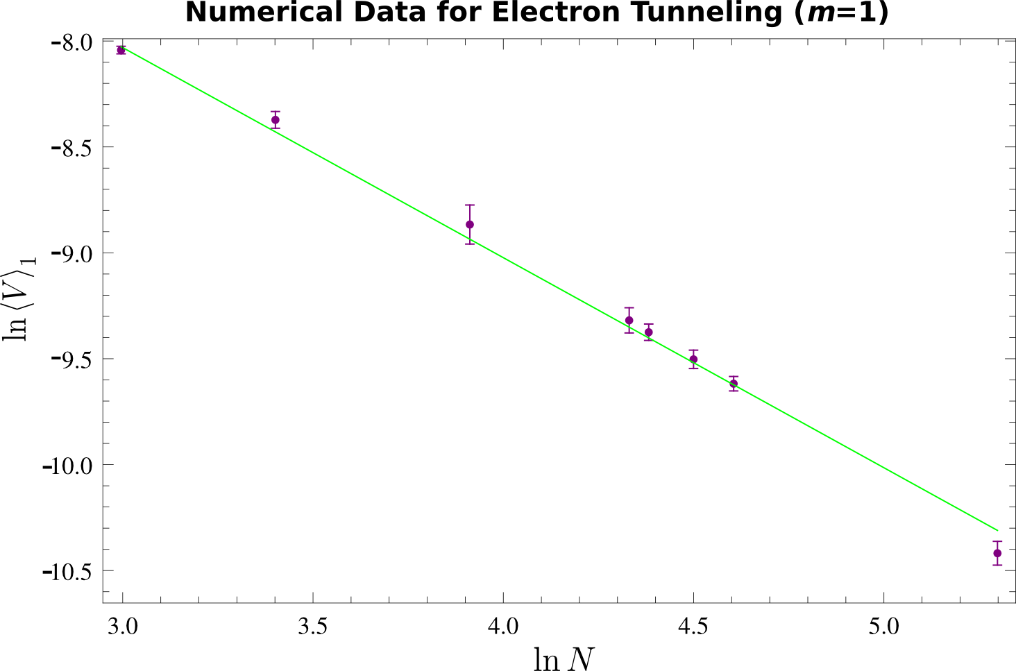
Figure 2: Curve for the logarithm of the zero mode quasiparticle tunnelling operator versus the logarithm of $N$ as calculated using Monte Carlo for filling factor $\nu=m^{-1}=1$. The purple points are the plots from the Monte Carlo data whilst the green, linear curve is the line of best fit as shown in equation (35).

The data set plotted on Figure 2 is fitted to straight a line where the gradient of the line for $\nu=1$ is given by,

$$\frac{\mathrm{d}\ln\left\langle V\right\rangle_{1}}{\mathrm{d}\ln N}=-0.99\pm 0.02\quad\quad(\textrm{for}\quad\nu=1)$$ (35)

The tunnelling matrix elements obviously have a system size dependence. Therefore when comparing these numerical results to the effective theory results for the tunnelling operator, operator ordering defined in (12) must be imposed for a constant $t_{p}$.

In the simulations, the impurity was placed at position $b$ along the real axis and so in the effective theory calculation $\xi=0$ and $R=|b|$. These parameters allow us to drop the absolute value of the matrix elements since the phase terms drop out anyway. Setting $p=\chi=1$ in (14) gives

$$\frac{\mathrm{d}\ln\left\langle A_{1}\right\rangle}{\mathrm{d}\ln N}=-0.96\quad\quad(\textrm{for}\quad\nu=1).$$ (36)

Comparing (36) to (35) shows that the effective theory, when using non-normal ordered operators does match the microscopic computations for the zero mode tunnelling matrix elements. The value of the gradient of the plot in Figure 2 as predicted from the effective theory is slightly out of the range of errors in the microscopic calculation. Possible reasons for this will be discussed after the results have been presented for the $\nu=1/3$ filling fraction.

3.3 Tunnelling Results for $\nu=1/3$

For the filling factor $\nu=1/3$ tunnelling matrix elements were computed for both a quasiparticle ($\chi=1$) and an electron ($\chi=3$) tunnelling across the bulk. Method 1 (21) was used for the quasiparticle tunnelling case and method 2 (34) for electron tunnelling. The data from both MC simulations is presented on a log-log plot in Figure 3.

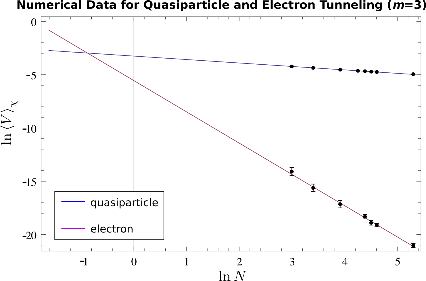
Figure 3: Curve for the logarithm of the zero mode quasiparticle tunnelling operator versus the logarithm of $N$ as calculated using MC for filling factor $\nu=m^{-1}=1/3$. The black points are the plots from the MC data for $\chi=1$ and $\chi=3$ whilst the blue and purple curves are lines of best fit shown in equations (37) and (39) respectively.

The gradient of linear curve fitted to the $\chi=1$ data set is;

$$\frac{\mathrm{d}\ln\left\langle V\right\rangle_{1}}{\mathrm{d}\ln N}=-0.325\pm 0.001\quad\quad(\textrm{for}\quad\nu=1/3).$$ (37)

Following similar arguments to those given in the results section for $\nu=1$; the effective theory prediction for the tunnelling matrix elements for a quasiparticle transferred across the bulk is

$$\frac{\mathrm{d}\ln\left\langle A_{1}\right\rangle}{\mathrm{d}\ln N}=-0.333\quad\quad(\textrm{for}\quad\nu=1/3).$$ (38)

Comparing (38) to (37); the effective theory does predict the correct scaling behaviour for the zero mode tunnelling matrix elements from the tunnelling Hamiltonian with non-normal ordered operators. Similar to the case for $\chi=1$ however, the result is slightly out of the error range of the microscopic calculations.

A possible reason for this could be related to the fact that to over come the phase problem in the original integral (17) the cumulant expansion was used. Obviously only a finite number of terms in the expansion could be computed numerically and this will produce a systematic error in the value of $\left\langle V\right\rangle_{1}$ for $\nu=1$ and $\nu=1/3$ that could account for the differences in the predicted value from the effective theory and the computed value from the microscopic theory. The cumulant expansion was terminated when the magnitude of the next term in the expansion could no longer be resolved due to the MC error. The number of terms kept varied for different computations and was dependent on the number of electrons $N$ in the system. It can be seen when comparing Figures 3 and 2 that the errors for the simulation for $\nu=1/3$ are smaller than those for $\nu=1$. This is due to the fact that the cumulant expansion decayed much faster for $\nu=1/3$ than $\nu=1$ and so fewer terms in the expansion for $\nu=1/3$ were kept.

The data for electron tunnelling ($\chi=3$) has also been fitted to a linear curve in Figure 3. The gradient of the line is given by;

$$\frac{\mathrm{d}\ln\left\langle V\right\rangle_{3}}{\mathrm{d}\ln N}=-3.03\pm 0.09\quad(\nu=1/3).$$ (39)

From (14), the effective theory prediction from the non-normal ordered tunnelling Hamiltonian can be extracted for electron tunnelling in the FQH state $\nu=1/3$.

$$\frac{\mathrm{d}\ln\left\langle A_{3}\right\rangle}{\mathrm{d}\ln N}=-3.00\quad(\nu=1/3).$$ (40)

For the case of an electron tunnelling across the bulk of a FQH device the effective theory predictions for the scaling of the zero mode matrix elements match the microscopic computations and are well within the error range. In Figure 3 the curves describing the MC data set for a quasiparticle and an electron tunnelling have been extrapolated such that the point of intersection of the two curves can be seen. Interestingly, the point at which the intersect occurs is when $N<1$ and therefore from the graph we see that at all physically possible system sizes the electron tunnelling process is always less relevant than the quasiparticle tunnelling process.

4 Summary and Conclusions

This work has investigated the zero mode tunnelling matrix elements due to an impurity in the bulk which have been computed as a function of system size, $N$ and then compared to the effective theory predictions for the tunnelling operators. In the first section the effective theory predictions were discussed. The quasiparticle operators from the Luttinger liquid theory of FQH edge states were used to calculate the zero mode matrix elements of the tunnelling operators $A_{p}$, where $p$ corresponded to the number of quasiparticles tunnelling at the impurity. These matrix elements were calculate using two types of ordering of quasiparticle operators. The first type was the usual definition of normal ordering defined in (10) were it was found that only the tunnelling parameter $t_{p}$ could contain system size dependence. The second type of ordering considered was when the operators were not normal ordered, as defined in (12). These matrix elements did show signs of system size dependence. To investigate which scaling of the tunnelling parameters $t_{p}$ best describe the tunnelling events in a FQH system a microscopic calculation was performed.

This microscopic calculation was based on the Laughlin states of the FQHE and was the subject of section II. The microscopic formula that describes the process for the tunnelling of $\chi$ particles due to the impurity inserted in to the bulk is given by $\left\langle V\right\rangle_{\chi}$ in (17). The only known way of calculating such integrals in (17) was by using numerical methods. The MC method was chosen for the computation of $\left\langle V\right\rangle_{\chi}$ though to directly calculate this average would not be very efficient since it is an average over a complex number which introduces a phase problem to the simulation.

Two methods were found to overcome this problem. Method 1. used MC to calculate the cumulant expansion of a function related to $\left\langle V\right\rangle_{\chi}$ and was suitable only for $\chi\leq 1$. Method 2. to overcome the phase problem was applicable only for $\chi=\nu^{-1}$ in which case the matrix elements in $\left\langle V\right\rangle_{\chi}$ could be written in terms of absolute values of complex numbers thus avoiding any phase problems.

Finally, the results of the MC calculations for $\left\langle V\right\rangle_{\chi}$ were presented and compared to the effective theory predictions of the tunnelling behaviour. It was found that the tunnelling Hamiltonian predicted by the effective theory is an accurate representation of the effects on the zero modes of the edges when an impurity is inserted into the bulk of a $\nu=1/3$ Laughlin state. Thus the Luttinger liquid model at some potential barrier has the same physics as a QPC inserted into a FQH device, which is something that has been assumed to be correct but not rigorously tested microscopically. When increasing the system sizes of the FQH device the electron operator plays a less important role than that of the quasiparticle operator. This can be seen for all system sizes and supports previous works mentioned in the introduction when the the electron tunnelling term is dropped in comparison to the quasiparticle tunnelling process. However, a match between the numerical data and the predictions made from the tunnelling Hamiltonian could only be obtained using a specific ordering for the operators. If one wishes to make the tunnelling Hamiltonian normal ordered then there must be a normalisation factor included in the definition of the quasiparticle and electron operators. The behaviour of the tunnelling Hamiltonian using such operators has also been shown to be well behaved physically, namely the operator is local in the sense that its correlation function is system-size independent.

References

- Tsui et al. (1982) D. C. Tsui, H. L. Stormer, and A. C. Gossard, Phys. Rev. Lett. 48, 1559 (1982).
- Laughlin (1983) R. B. Laughlin, Phys. Rev. Lett. 50 (1983), URL http://link.aps.org/doi/10.1103/PhysRevLett.50.1395.
- Wen (1990) X. G. Wen, Phys. Rev. B 41 (1990), URL http://link.aps.org/doi/10.1103/PhysRevB.41.12838.
- Chang (2003) A. M. Chang, Rev. Mod. Phys. 75, 1449 (2003), URL http://link.aps.org/doi/10.1103/RevModPhys.75.1449.
- Kane and Fisher (1992a) C. Kane and M. P. Fisher, Physical Review B 46, 15233 (1992a).
- Kane and Fisher (1992b) C. L. Kane and M. P. A. Fisher, Phys. Rev. B 46, 7268 (1992b), URL http://link.aps.org/doi/10.1103/PhysRevB.46.7268.
- Kane and Fisher (1992c) C. L. Kane and M. P. A. Fisher, Phys. Rev. Lett. 68, 1220 (1992c), URL http://link.aps.org/doi/10.1103/PhysRevLett.68.1220.
- Furusaki and Nagaosa (1993) A. Furusaki and N. Nagaosa, Phys. Rev. B 47, 4631 (1993), URL http://link.aps.org/doi/10.1103/PhysRevB.47.4631.
- Moon et al. (1993) K. Moon, H. Yi, C. L. Kane, S. M. Girvin, and M. P. A. Fisher, Phys. Rev. Lett. 71, 4381 (1993), URL http://link.aps.org/doi/10.1103/PhysRevLett.71.4381.
- Gogolin et al. (2004) A. Gogolin, A. Nersesyan, and A. Tsvelik, Bosonization and Strongly Correlated Systems (Cambridge University Press, 2004), ISBN 9780521617192, URL http://books.google.co.uk/books?id=BZDfFIpCoaAC.
- Milliken et al. (1996) F. Milliken, C. Umbach, and R. Webb, Solid State Communications 97, 309 (1996), ISSN 0038-1098, URL http://www.sciencedirect.com/science/article/pii/0038109895001816.
- Roddaro et al. (2004) S. Roddaro, V. Pellegrini, F. Beltram, G. Biasiol, and L. Sorba, Phys. Rev. Lett. 93, 046801 (2004), URL http://link.aps.org/doi/10.1103/PhysRevLett.93.046801.
- Chang et al. (1996) A. M. Chang, L. N. Pfeiffer, and K. W. West, Phys. Rev. Lett. 77, 2538 (1996), URL http://link.aps.org/doi/10.1103/PhysRevLett.77.2538.
- Kane and Fisher (1994) C. L. Kane and M. P. A. Fisher, Phys. Rev. Lett. 72, 724 (1994), URL http://link.aps.org/doi/10.1103/PhysRevLett.72.724.
- Saminadayar et al. (1997) L. Saminadayar, D. C. Glattli, Y. Jin, and B. Etienne, Phys. Rev. Lett. 79, 2526 (1997), URL http://link.aps.org/doi/10.1103/PhysRevLett.79.2526.
- dePicciotto et al. (1997) R. dePicciotto, M. Reznikov, M. Heiblum, V. Umansky, G. Bunin, and D. Mahalu, NATURE 389, 162 (1997), ISSN 0028-0836.
- Dolev et al. (2010) M. Dolev, Y. Gross, Y. C. Chung, M. Heiblum, V. Umansky, and D. Mahalu, Phys. Rev. B 81, 161303 (2010).
- Baer et al. (2014) S. Baer, C. Rössler, T. Ihn, K. Ensslin, C. Reichl, and W. Wegscheider, Phys. Rev. B 90, 075403 (2014), URL http://link.aps.org/doi/10.1103/PhysRevB.90.075403.
- Yang and Feldman (2013) G. Yang and D. E. Feldman, Phys. Rev. B 88, 085317 (2013), URL http://link.aps.org/doi/10.1103/PhysRevB.88.085317.
- Fendley et al. (1995) P. Fendley, A. W. W. Ludwig, and H. Saleur, Phys. Rev. Lett. 74, 3005 (1995), URL http://link.aps.org/doi/10.1103/PhysRevLett.74.3005.
- Guyon et al. (2002) R. Guyon, P. Devillard, T. Martin, and I. Safi, Phys. Rev. B 65, 153304 (2002), URL http://link.aps.org/doi/10.1103/PhysRevB.65.153304.
- Kane (2003) C. L. Kane, Phys. Rev. Lett. 90, 226802 (2003), URL http://link.aps.org/doi/10.1103/PhysRevLett.90.226802.
- Safi et al. (2001) I. Safi, P. Devillard, and T. Martin, Phys. Rev. Lett. 86, 4628 (2001), URL http://link.aps.org/doi/10.1103/PhysRevLett.86.4628.
- Law et al. (2006) K. T. Law, D. E. Feldman, and Y. Gefen, Phys. Rev. B 74, 045319 (2006), URL http://link.aps.org/doi/10.1103/PhysRevB.74.045319.
- Vishveshwara (2003) S. Vishveshwara, Phys. Rev. Lett. 91, 196803 (2003), URL http://link.aps.org/doi/10.1103/PhysRevLett.91.196803.
- Nayak et al. (1999) C. Nayak, M. P. A. Fisher, A. W. W. Ludwig, and H. H. Lin, Phys. Rev. B 59, 15694 (1999), URL http://link.aps.org/doi/10.1103/PhysRevB.59.15694.
- Ponomarenko and Averin (2004) V. V. Ponomarenko and D. V. Averin, Phys. Rev. B 70, 195316 (2004), URL http://link.aps.org/doi/10.1103/PhysRevB.70.195316.
- Jonckheere et al. (2005) T. Jonckheere, P. Devillard, A. Crépieux, and T. Martin, Phys. Rev. B 72, 201305 (2005), URL http://link.aps.org/doi/10.1103/PhysRevB.72.201305.
- Haldane (1983) F. D. M. Haldane, Phys. Rev. Lett. 51, 605 (1983), URL http://link.aps.org/doi/10.1103/PhysRevLett.51.605.
- A. Boyarsky (2004) O. R. A. Boyarsky, Vadim V. Cheianov, arXiv:cond-mat/0402562v2 [cond-mat.mes-hall] (2004).
- Ivan P. Levkivskyi (2010) E. V. S. Ivan P. Levkivskyi, Juerg Froehlich, arXiv:1005.5703v1 [cond-mat.mes-hall] (2010).
- Metropolis et al. (1953) N. Metropolis, A. W. Rosenbluth, M. N. Rosenbluth, A. H. Teller, and E. Teller, The Journal of Chemical Physics 21, 1087 (1953), URL http://scitation.aip.org/content/aip/journal/jcp/21/6/10.1063/1.1699114.