Comparison of computer-algebra strong-coupling perturbation theory and dynamical mean-field theory for the Mott-Hubbard insulator in high dimensions

Abstract

We present a large-scale combinatorial-diagrammatic computation of high-order contributions to the strong-coupling Kato-Takahashi perturbation series for the Hubbard model in high dimensions. The ground-state energy of the Mott-insulating phase is determined exactly up to the 15–th order in $1/U$. The perturbation expansion is extrapolated to infinite order and the critical behavior is determined using the Domb-Sykes method. We compare the perturbative results with two dynamical mean-field theory (DMFT) calculations using a quantum Monte Carlo method and a density-matrix renormalization group method as impurity solvers. The comparison demonstrates the excellent agreement and accuracy of both extrapolated strong-coupling perturbation theory and quantum Monte Carlo based DMFT, even close to the critical coupling where the Mott insulator becomes unstable.

I Introduction

The Kato-Takahashi strong-coupling perturbation theory (SCPT) [1; 2] and the dynamical mean-field theory (DMFT) [3; 4] are two powerful methods for studying strongly correlated quantum many-body systems such as the Mott insulating phase [5; 6] found in the Hubbard model [7; 8; 9] with on-site interaction $U$. In high dimensions the Kato-Takahashi SCPT can be calculated exactly up to high orders in $1/U$ using a combinatorial-diagrammatic approach [10; 11] while the DMFT scheme becomes exact in principle. Early comparisons of both methods [12; 10] showed a very good agreement deep in the Mott insulating phase. However, they let some open questions about the relative accuracy of different impurity solvers for DMFT and the properties of the Mott insulating phase close to the critical coupling $U_{c}$ where it becomes unstable. Here, we report on a large-scale computer-algebra calculation of higher orders in the SCPT series expansion and the resolution of this issue.

I.1 Mott insulator and Hubbard model

The nature of Mott insulators without long-range magnetic order is a long-standing open problem in the theory of strongly correlated quantum systems. Theoretically, Mott insulating phases can be found in strongly interacting fermion [5; 6] or boson [13] systems as well as in fermion-boson mixtures [14]. Experimentally, non-magnetic Mott insulators have been found in a layered organic insulator [15]. In this triangular-lattice material, the frustration of the antiferromagnetic spin exchange coupling prevents the formation of a long-range magnetic order. A Mott insulator phase can also be realized in an atomic gas trapped in an optical lattice [16; 17]. Despite decades of extensive research, the properties of Mott insulators and, more generally, the transition from a Mott insulator to a metallic (fermion system) or superfluid (boson system) phase are only partially understood and thus actively investigated.

The Hubbard model with repulsive on-site interaction $U\geq 0$ and nearest-neighbor hopping term $t\geq 0$ is a basic lattice model for studying the physics of strongly interacting electrons, in particular the Mott metal-insulator transition. [6] At half filling (one electron per lattice site) the ground state is a Mott insulator for strong interaction $U/t$, while it is a Fermi gas in the non-interacting limit $U=0$. Thus, the system must undergo a metal-insulator transition at some coupling $U^{\text{MIT}}_{c}\geq 0$. If the lattice geometry (defined by hopping integrals between lattice sites) causes a strong frustration of the effective antiferromagnetic exchange coupling between electron spins, the ground state is paramagnetic. Thus, this model can describe the transition from a paramagnetic Mott insulator to a metallic state. The Bose-Hubbard model is an extension of the Hubbard model to boson systems, which can be used to describe the transition from a Mott insulator to a superfluid. [17]

Here we consider the Hamiltonian for interacting electrons

$$H = T+UD$$

$$T = -\sum_{\langle i,j\rangle}\sum_{\sigma=\uparrow,\downarrow}\frac{t_{\sigma}}{\sqrt{Z}}\left(c^{{\dagger}}_{i,\sigma}c^{\phantom{{\dagger}}}_{j,\sigma}+c^{{\dagger}}_{j,\sigma}c^{\phantom{{\dagger}}}_{i,\sigma}\right)$$ (1)

$$D = \sum_{i}n_{i,\uparrow}n_{i,\downarrow}$$

where $c^{{\dagger}}_{i,\sigma}$ and $c^{\phantom{{\dagger}}}_{i,\sigma}$ are the standard fermion creation and annihilation operators for an electron with spin $\sigma$ on the site with index $i$ and $n_{i,\sigma}=c^{{\dagger}}_{i,\sigma}c^{\phantom{{\dagger}}}_{i,\sigma}$ are the local density operators. To reach the limit of infinite dimensions, we choose a Bethe lattice with connectivity $Z$ in the limit $Z\to\infty$. Thus, the last sum in (1) runs over the $L$ lattice sites while the first sum runs over the $LZ/2$ pairs of nearest-neighbor sites. We restrict the present study to a half-filled system (i.e., one electron per site on average). The Hubbard model corresponds to equal hopping terms for both spins $t_{\uparrow}=t_{\uparrow}=t$ while the Falicov-Kimball model[18] corresponds to a single mobile electron species $t_{\uparrow}=t>0$ and $t_{\downarrow}=0$. We will set the unit of energy by $t\equiv 1$.

I.2 Dynamical mean-field theory

DMFT and its generalizations have become a leading approach for studying correlated electronic systems. [3; 4] They have been combined with the density functional theory [4; 19] to perform first-principles calculations. This DFT+DMFT approach is increasingly used to investigate materials with strong electronic correlations such as transition metals and their oxides. More recently, the application of DMFT to quantum chemistry problems has been explored. [20]

The Mott metal-insulator transition in the Hubbard model has been extensively investigated with DMFT. [3; 21; 22; 12; 23; 24] On a Bethe lattice with infinite coordination number, DMFT studies have revealed a first-order quantum phase transition from a Fermi liquid to a Mott insulator as $U$ increases. The ground state is metallic up to a critical coupling $U^{\text{MIT}}_{c}$ (which is close to $5.8$ according to QMC-DMFT calculations [22]) and becomes insulating above this value. However, the Mott insulating state remains metastable down to a critical coupling $U_{c}<U^{\text{MIT}}_{c}$ where the Mott-Hubbard gap closes. Thus, it still influences the system properties for $U_{c}<U<U^{\text{MIT}}_{c}$ and in real systems, it should be observable in experiments such as time-resolved spectroscopy.

In the DMFT approach, a bulk system is mapped onto an effective self-consistent quantum impurity system. In the case of the Hubbard model, this is the well-known single impurity Anderson model (SIAM). This mapping becomes exact in the limit of infinite dimensions or coordination number. However, solving the quantum impurity problem is a very hard task in most cases. Various ``impurity solvers'' can be used to compute the SIAM properties numerically. For instance, numerical renormalization group (NRG) [21], density matrix renormalization group (DMRG) [25; 12; 23; 24], and quantum Monte Carlo (QMC) [10; 22] methods have been used successfully for this purpose. Thus, in practice, one has to solve the self-consistent impurity problem numerically and recursively. This introduces errors which are difficult to estimate within the DMFT scheme. Therefore, reliable results obtained with other methods are highly desirable to validate the DMFT approach and evaluate its accuracy, even in the limit of infinite dimensions. So far, besides DMFT computations, most reliable results for the Hubbard model in the limit of high dimensions have been obtained using weak [26; 25] and strong coupling perturbation theory [12; 10; 11]. Additionally, the Kato-Takahashi SCPT can be used to solve the DMFT self-consistency equation. [27]

I.3 Strong-coupling perturbation theory

Series expansion methods, especially perturbative approaches, constitute basic theoretical tools of physics. [28; 29; 30; 31; 32; 33; 34] They are often used to investigate strongly correlated lattice models such as the Hubbard model. An attractive feature of these methods is that they are often well suited for the use of high-performance computer algebra. Thus, one can take advantage of the computational power of modern supercomputers without losing the rigor of analytical calculations. This can be a decisive advantage over most numerical approaches, which usually have to deal with various issues brought by finite-precision algorithms and floating-point arithmetic.

In principle, the Kato-Takahashi perturbation expansion provides us with a systematic method for calculating the properties of the Mott insulator in powers of $1/U$. In practice, the number of diagrams contributing to $n$-th order increases exponentially with $n$ and thus calculations become rapidly too complex. Several years ago, a direct manual calculation yielded the ground-state energy of (1) up to the 4-th order and the local Green's function up to second order in $1/U$. [35; 36; 37] These results agree well with DMRG-based DMFT simulations for $U\geq 6$. [12] Later, an combinatorial-diagrammatic algorithm was developed to calculate a given order exactly using computer algebra. This method allowed one of us to compute the ground-state energy exactly up to the 11-th order in $1/U$ using moderate computational resources. [10; 11] The results agree very well down to $U=4.8$ with DMFT data obtained using a QMC method [10] or a DMRG method [12] as impurity solver. However, these studies reached different conclusions regarding the critical coupling $U_{c}$ where the Mott insulator becomes unstable, and the related critical exponent $\tau$. Combining QMC-DMFT and SCPT results the first study [10] claimed that $U_{c}\approx 4.78$ (in agreement with other DMFT calculations [23; 21; 22]) and $\tau\approx 7/2$ while the DMRG-DMFT-based study [12] concluded that $U_{c}\approx 4.45$ and $\tau\approx 5/2$. In addition, a critical coupling $U_{c}\approx 4.406$ was deduced from a perturbative calculation of the Mott-Hubbard gap within the DMFT approach. [27]

Unfortunately, even the most recent SCPT study (up to 11-th order in $1/U$) [11] was not sufficient to discriminate between the QMC and DMRG data close to $U_{c}$. It is well known that a series expansion truncated at any finite order becomes increasingly unreliable as one approaches a critical point (i.e., an analytical singularity) and that taking higher-order into account improves the reliability. Thus, in this paper we present a large-scale computer-algebra calculation which allows us to obtain the ground-state energy up to the 15-th order in $1/U$ using the combinatorial-diagrammatic approach. The comparison of SCPT and DMFT results reveals that QMC-DMFT agrees much better than DMRG-DMFT with the 15-th order perturbation theory close to the critical regime (down to $U=4.8$). In addition, extrapolating the perturbation expansion to infinite order using the Domb-Sykes method [38; 39] allows us to determine critical coupling $U_{c}\approx 4.76$ and critical exponent $\tau\approx 3.45$ very precisely. This critical coupling also agrees with previous DMFT calculations. [10; 22; 21; 23] Moreover, we find that the ground-state energies calculated with the extrapolated SCPT and the QMC-DMFT agree perfectly (within $10^{-7}$ of the band width) even extremely close to the critical coupling, e.g. for $U-U_{c}\approx 0.04$.

The rest of this paper is structured as follows. The high-performance computer-algebra SCPT is described in the next section. Section III presents the comparison of the SCPT results with the DMRG-DMFT and QMC-DMFT data as well as the extrapolated perturbation theory. Finally, the perspective for further development and applications of the combinatorial-diagrammatic SCPT are discussed in Sec. IV.

II Computer-algebra SCPT

II.1 Kato-Takahashi series expansion

The ground-state energy per lattice site $E$ of the Hamiltonian (1) can be written as a series in power of $1/U$ using the Kato-Takahashi strong-coupling perturbation theory. [1; 2] At $U=\infty$ (or equivalently $t=0$) the ground-state energy is $E_{0}=0$ and the corresponding eigenstates have exactly one electron localized on each lattice site. As the spin orientation does not change the energy, the ground state is degenerate. We denote by $\mathcal{H}_{0}$ the corresponding eigenspace. Its dimension is $2^{L}$ for an $L$-site lattice. Let $P$ be the projection operator onto the lowest-energy eigenspace of the Hamiltonian (1) at finite $U$. (Obviously, $P$ is the projector onto $\mathcal{H}_{0}$ for $U=\infty$.) Using the generic Kato perturbation theory, Takahashi showed for the Hubbard model in the strong-coupling limit that this operator can be written as a power series in $1/U$

$$P=-\sum_{n=0}^{\infty}\frac{1}{U^{n}}{\sum_{\{k_{r}\}}}S^{k_{1}}TS^{k_{2}}T\cdots TS^{k_{n+1}}$$ (2)

with integers $k_{r}\geq 0$ such that $k_{1}+k_{2}+\cdots+k_{n+1}=n$. At half filling, this power series has a finite convergence radius $U^{-1}_{R}>0$ and that depends on the lattice properties. The operators $S^{k}$ are defined by

$$S^{k}=\begin{cases}\displaystyle{-P_{0}}&\text{for $k=0$}\\ \displaystyle{\sum_{d=1}^{L}\frac{1}{(-d)^{k}}P_{d}}&\text{for $k>0$}\end{cases}$$ (3)

where $P_{d}$ is the projector on the subspace of states with exactly $d$ doubly occupied sites.

Let us assume that $\left|\phi_{0}\right\rangle$ is a state in $\mathcal{H}_{0}$ with the property $P\left|\phi_{0}\right\rangle\neq 0$. (There must be at least one such state if the series expansion for $P$ has a finite convergence radius.) Then the ground-state energy for finite $1/U$ is given by

$$E=\frac{1}{L}\frac{\left\langle\phi_{0}|PHP|\phi_{0}\right\rangle}{\left\langle\phi_{0}|P|\phi_{0}\right\rangle}.$$ (4)

Using (2), we can expand this energy in power of $1/U$

$$E=\sum_{n=1}^{\infty}\frac{a_{n}}{U^{n}}$$ (5)

for $U_{R}<U<\infty$. Although one cannot write closed formula for the coefficients $a_{n}$ in general, they are completely defined by the equations (2), (3), and (4) for a given lattice and a given hopping operator $T$.

II.2 Combinatorial-diagrammatic approach

A combinatorial-diagrammatic approach was developed by one of us to evaluate the coefficients $a_{n}$ for the Hubbard and Falicov-Kimball models on a Bethe lattice with an infinite coordination number. [10; 11] Here we summarize the key ideas which are necessary to understand our new implementation of this approach and we refer the reader to the original publications for more details. Expanding the projector (2) in the energy (4), we see that the coefficients $a_{n}$ are given by sums of expectation values of the form

$$\left\langle\phi_{0}|TP_{d_{1}}TP_{d_{2}}TP_{d_{3}}\cdots T|\phi_{0}\right\rangle,$$ (6)

which are called processes. Different sets $\{k_{r}\}$ and $\{d_{r}\}$ in eqs. (2), (3), and (6) correspond to different processes. The number of different sets $\{k_{r}\}$ in the projector (2) is $\binom{2n}{n}$ for the $n$–th order and thus increases exponentially as $\frac{4^{n}}{\sqrt{\pi n}}$ for high orders $n$. The number of different sets $\{d_{r}\}$ scales as $L^{n-1}$. Thus the number of possible processes increases exponentially fast with the order $n$.

The state $\left|\phi_{0}\right\rangle$ is an eigenstate of the double occupation operator $D$ and thus has a precise number of doubly occupied sites (zero at half filling) while the hopping operator $T$ can change the number of doubly occupied sites by at most one. Consequently, only some particular sets $\{d_{r}\}$ can yield a non-zero expectation value (6). Then using the definition of the hopping operator $T$ in Eq. (1) each process can be evaluated as the sum of simple expectation values

$$\left\langle\phi_{0}\left|c^{{\dagger}}_{i_{1},\sigma_{1}}c^{\phantom{{\dagger}}}_{i_{2},\sigma_{2}}c^{{\dagger}}_{i_{3},\sigma_{3}}c^{\phantom{{\dagger}}}_{i_{4},\sigma_{4}}\cdots c^{\phantom{{\dagger}}}_{i_{2l},\sigma_{2l}}\right|\phi_{0}\right\rangle$$ (7)

(called sequences) over lattice sites and spin indices. The sequence length is $1\leq l\leq n+1$. The number of different sequences in a process increases exponentially fast with the order $n$, roughly as $(2ZL)^{l}$ for a process containing $l$ hopping operators $T$.

Table 1: Number of different non-zero processes $N_{p}$, number of sequences $N_{s}$ in (10), series coefficients $a_{n}$, number of processors used, wall time of calculation, and the total amount of required memory for the non-trivial orders $n$ from 1 to 15 using the preprocessing technique as well as estimates for the next non-trivial order $n=17$ without preprocessing

$n$	$N_{p}$	$N_{s}$	$a_{n}$	proc.	time		memory
							(Gb)
$1$	$1$	$2$	$\displaystyle{-\frac{1}{2}}$
$3$	$2$	$20$	$\displaystyle{-\frac{1}{2}}$
$5$	$4$	$648$	$\displaystyle{-\frac{19}{8}}$
$7$	$14$	$45472$	$\displaystyle{-\frac{593}{32}}$
$9$	$48$	$5644880$	$\displaystyle{-\frac{23877}{128}}$	$1$	$6$	sec.	$<1$
$11$	$193$	$1099056000$	$\displaystyle{-\frac{4496245}{2048}}$	$1$	$18$	min.	$<1$
$13$	$795$	$310007943616$	$\displaystyle{-\frac{1588528613}{55296}}$	$128$	$12$	min.	$36$
$15$	$3412$	$119777421416192$	$\displaystyle{-\frac{12927125815211}{31850496}}$	$128$	$77$	hours	$528$
$17$	$14803$	$<804658\cdot 10^{11}$		$262144$	$13$	days	$131$

Therefore, the evaluation of the coefficients $a_{n}$ in the series (5) is a hard computational problem. However, the computational cost can be greatly reduced if one identifies without explicit calculation the many processes and sequences which vanish or are equivalent. For instance, processes can be gathered into a small number of classes defined by the positions $r$ of the indices $k_{r}=0$ in the list $\{k_{r}\}$. Then the processes in a given class are only compatible with particular sets $\{k_{r}\}$ and $\{d_{r}\}$ as well as a reduced number of sequences because an intermediate state

$$\left.\left.c^{{\dagger}}_{i_{2r+1},\sigma_{2r+1}}c^{\phantom{{\dagger}}}_{i_{2r+2},\sigma_{2r+2}}c^{{\dagger}}_{i_{2r+3},\sigma_{2r+3}}\cdots c^{\phantom{{\dagger}}}_{i_{2l},\sigma_{2l}}\right|\phi_{0}\right\rangle$$ (8)

without any doubly occupied site must be reached every time that $k_{r}=0[\Leftrightarrow d_{r}=0$ in Eq. (6)]. The actual number $N_{p}$ of inequivalent non-zero processes in our implementation is given in the second column of Table 1 for several orders $n$.

The above discussion is valid for any lattice. On a Bethe lattice with an infinite coordination number $Z$, however, the evaluation of sequences and processes can be considerably simplified. First, it was shown [36] that the degeneracy of the singlet ground state for $U=\infty$ is not lifted up to the third order in $1/U$ (if one excludes long-range spin orders such as anti-ferromagnetism). Assuming that this holds for all orders, we can use any singlet state $\left|\phi_{0}\right\rangle\in\mathcal{H}_{0}$ or, equivalently, an average over an orthonormal basis of the singlet subspace in $\mathcal{H}_{0}$. (This averaging greatly simplifies the evaluation of sequences as we will see below.) Moreover, an expectation value (7) vanishes unless each creation operator $c^{{\dagger}}_{i,\sigma}$ in the sequence is matched by a corresponding annihilation operator $c^{\phantom{{\dagger}}}_{i,\pm\sigma}$. Thus the site set $\{i_{r}\}$ in a sequence (7) describes one or more closed paths on the lattice. As the operator $T$ contains hoppings between nearest-neighbor sites only, each segment of the path connects two nearest-neighbor sites. Moreover, as loops are not possible on a Bethe lattice, the path is self-retracing and any nearest-neighbor bond can only appear an even number of times in a closed path. Finally, segments occurring more than twice yield contributions of the order of $1/Z$ or smaller and thus are negligible in the limit of an infinite coordination number.

Some other generic properties can be used to further simplify the problem. As the total energy must be extensive, disconnected paths resulting from the expansion of numerator and denominator in the ratio (4) must compensate each other and thus only sequences corresponding to a single connected path of length $l=n+1$ yield non-zero contributions in the $n$–th order. This property is sometimes called a linked-cluster theorem but in the present context it is more a physical argument than a mathematical theorem. It was only proven exactly up to the fifth order in $1/U$ in Ref. 36. A detailed analysis of the linked-cluster theorem within the Kato-Takahashi perturbation theory also indicates that it should be valid for the Mott-insulating phase of the half-filled Hubbard model. [34; 40] Finally, all lattice sites are equivalent as we assume that the lattice is infinitely large ($L\rightarrow\infty$).

In summary, the only non-zero contributions to processes (6) come from sequences (7) corresponding to a single, closed, and self-retracing path of even length $l=n+1$ through $l/2$ different bonds and $l/2+1$ different sites. This has three important consequences. First, only processes corresponding to an even power of the hopping operator $T$, or equivalently an odd power of $1/U$, contribute to the ground-state energy at half filling.

Second, after reordering the fermion operators, any contributing sequences can be written as a correlation function

$$\left\langle\phi_{0}\left|\prod_{r=1}^{l}c^{{\dagger}}_{i_{r},\sigma_{r}}c^{\phantom{{\dagger}}}_{i_{r},\sigma^{\prime}_{r}}\right|\phi_{0}\right\rangle$$ (9)

between all sites in a path of length $l$. Computing the average of the energy (4) over an orthonormal basis of the singlet subspace in $\mathcal{H}_{0}$ reduces to averaging these correlation functions. In the thermodynamic limit $L\rightarrow\infty$ all spin configurations of a finite cluster are equiprobable if one averages over all singlet states of the full system. Thus we can simply compute the mean value of the correlation function over both spin states $\sigma=\uparrow,\downarrow$ at each site in the path. We find then that the average value of a correlation function depends only on the path length $l$ (and so on the order $n$) and is simply a rational number $2^{-(n+3)/2}$.

Third, the distinct linked clusters occurring in contributing sequences can be represented one to one by diagrams called Butcher trees.[11; 41] Generating all these clusters corresponds to generating all Butcher trees with $l/2+1=(n+3)/2$ nodes. We have to use colored Butcher trees with four distinct colors corresponding to the four possible states (unoccupied, spin-$\uparrow$, spin-$\downarrow$, and doubly occupied) of an electronic site to represent the initial spin configurations in $\left|\phi_{0}\right\rangle$ and the intermediate states (8) of a sequence. After constructing all $n$–th order Butcher trees, all possible sequences on them can be generated starting from the graph root using a recursive electron hopping procedure, which takes into account the physical restrictions such as the Pauli principle. Therefore, the evaluation of the coefficients $a_{n}$ in the series (5) is reduced to a (hard) combinatorial-diagrammatic problem.

II.3 High-performance computer-algebra implementation

A combinatorial-diagrammatic approach was used to calculate the coefficients $a_{n}$ exactly up to $n=11$ for both the Hubbard model and the Falicov-Kimball model using a proof-of-concept computer program and moderate computer resources. [10; 11] Based on the original program, one of us (MP) has implemented a high-performance computer-algebra program that calculates the coefficients $a_{n}$ exactly for a given odd $n$ (as $a_{n}=0$ for all even $n$ at half filling). The coefficients are written

$$a_{n}=r\frac{2^{-(n+3)/2}}{n+1}\sum_{g}\sum_{s}S_{s}\left(\sum_{p}C_{p}\prod_{j=1}^{n}d_{j}^{-k_{j}}\right)$$ (10)

where $r=1$ for the Falicov-Kimball model and $r=2$ for the Hubbard model. The first sum runs over all $2^{(n-1)/2}$ process classes $g$. The sum over the index $s$ represents the sum over all sequences (7) which are compatible with the process class $g$. The sequences for the Falicov-Kimball model are a subset of those for the Hubbard model. A set of double occupancy number $\{d_{r}\}$ is associated with each sequence $s$ and $S_{s}=\pm 1$ is the overall sign of this sequence from the fermion commutation relations. The total number $N_{s}$ of all sequences in all classes is given in the third column of Table 1 up to the order $n=15$. The sum over the index $p$ in (10) represents the sum over all inequivalent elementary processes (6) in the class $g$. These processes are the same for the Falicov-Kimball model and the Hubbard model. A set of exponents $\{k_{r}\}$ is associated with each elementary process $p$ and $C_{p}$ gives the number of equivalent elementary processes. The total number $N_{p}$ of all processes in all classes is given in the second column of Table 1 up to the order $n=17$.

We see that $N_{s}$ increases faster than $n!$. This apparently disagrees with the above analysis which predicts at most an exponential increase of the number of processes and sequences with $n$. However, the exponential behavior is obtained for a finite lattice $L$ and a finite coordination number $Z$ and thus does not preclude a factorial behavior in the limits $L,Z\rightarrow\infty$. For orders up to $n=11$ the computation of (10) can be easily carried out on a workstation. Our optimized and parallelized implementation of this combinatorial-diagrammatic algorithm has allowed us to carry out the calculation up to the order $n=15$ using high-performance supercomputers.

This implementation represents about $3800$ lines of ANSI-C code (comments excluded). The program uses only integer numerics with a ``global'' denominator instead of slower rational numbers. Thus the coefficients $a_{n}$ are obtained as exact rational numbers. We have found that standard $64$-bit integers are enough up to the 13-th order but $128$-bit ones are required for the 15-th order. For the 17-th order, integers with $256$ bits or more would be necessary. In practice, we use the GNU Multiple Precision Arithmetic Library (GMP) [42], which provides integers of arbitrary length.

To optimize the program we have implemented the necessary algorithms as fast operations on our bit-coded data structures. These include standard combinatorial algorithms, e.g. for sorting and permuting, [43] as well as more specialized ones, e.g. for computing the overall sign from all fermion operator commutations in a sequence. Thus our implementation is self-contained and does not require any special software library except GMP. A further optimization of several algorithms was achieved thanks to an independent graph-theoretical analysis of the representation of sequences by colored Butcher trees. [44; 45] This analysis was carried out using the functional programming language Haskell, which provides a concise high-level mathematical environment for this purpose, e.g. native support for graph structures. In addition, we have used the On-Line Encyclopedia of Integer Sequences (OEIS) [46] to analyze the various integer sequences which occur in intermediate steps of the combinatorial-diagrammatic algorithm and thus verify some intermediate results. This analysis has also helped us to improve the overall program efficiency.

In contrast to the proof–of–concept implementation in Ref. 11, our implementation consists of a single program. To generate all contributing sequences $s$ in (10), it iterates in parallel over all initial states (i.e., spin configurations in $\left|\phi_{0}\right\rangle$) in an outer loop while an inner loop runs over all combinations of nearest-neighbor pairs using a recursive electron hopping procedure. A trade-off between CPU time and memory usage can be achieved if one initially calculates once and stores the possible sequence weights [i.e., the sum over the elementary processes $p$ in Eq. (10)] for all double occupancy sets $\{d_{r}\}$. Then during the summation over the sequences $s$, one uses the stored weight for the set $\{d_{r}\}$ corresponding to each sequence. This preprocessing of sequence weights yields a significant speed-up at the cost of a higher memory requirement. For instance, preprocessing reduces the CPU time by a factor $3.3$ for the 15-th order, which offsets the higher computational cost of the GMP library compared to fixed-length integers. Theoretically, the required memory for the sequence-generating subroutine increases from $\propto n^{2}$ without preprocessing to $\propto 4^{n}$ with preprocessing, while the main program needs a constant amount $\propto 2^{n}$. In addition, this method results in an unfavorable memory scaling in a parallel computation as the total memory now increases linearly with the number of processors while it remains almost constant without preprocessing. As an example, for the order $n=15$, $4$ Gb for each processor plus $16$ Gb of shared memory are used with preprocessing against only $16$ Gb overall without preprocessing.

Our code has been designed for running efficiently on parallel supercomputers. For an efficient handling of shared data by the specialized combinatorial functions, we have limited ourselves to symmetric multiprocessor (SMP) computer architectures so far. Due to the ideal data parallelism in our implementation as well as to a fine-tuned load balancing, the scaling behavior of the computing time is excellent on all tested machines, at least up to $510$ processor cores on a SGI Altix 4700 and up to $256$ processor cores on the much more powerful HP Integrity Superdome 2-32s. A simple analysis on basis of Amdahl's law gives $99.93\%$ code parallelism. [47]

Nevertheless, calculating the sum (10) for $n>11$ remain computationally demanding and we have to carry out large-scale calculations on SMP machines with hundreds of processors to obtain the 13–th and 15–th orders in $1/U$. The wall time used and the required memory are shown in Table 1 for calculations performed using the preprocessing method on a HP 9000 J6750 workstation (orders $n=9$ and $11$) and a HP Integrity Superdome 2-16s server (orders $n=13$ and $15$). In Table 1, we also show our estimates for the order $n=17$ using a massively parallel processing (MPP) supercomputer such as the IBM BlueGene/Q with $262144$ processors. Note that the preprocessing method could not be used on this computer system without modification because the available memory per processor would be too low.

The validity and performance of our program were also tested on the Falicov-Kimball model [18] using a state-of-the-art SMP supercomputer (HP Integrity Superdome X). As a result, we can confirm that there is no contribution to the ground-state energy (beyond the first order term) up to the 17–th order in $1/U$, i.e. 6 orders higher than in a previous work. [11] This test also allows us to estimate the computational cost for the 17-th order in the Hubbard model. It shows that $7.7$ Tb of memory would be required with preprocessing on the $240$ processor cores of the HP Integrity Superdome X and that the calculation would last more than one year (while the test for the Falicov-Kimball model only took $54$ hours). Therefore, the calculation of the next order in the Hubbard model series expansion does not seem to be possible with current SMP machines. Nevertheless, it appears to be technically possible with current MPP supercomputers such as the IBM BlueGene/Q, although we could not use the current implementation of the preprocessing and the computational cost, about $13$ days, would still be very high in practice.

III Results

III.1 Comparison of SCPT and DMFT

In Table 1, we present the coefficients $a_{n}$ of the power series for the ground-state energy (5) in the half-filled Hubbard model up to the order $n=15$. (Only coefficients for odd $n$ are listed as they vanish for all even $n$.) They agree with those obtained in previous works [10; 11] up to the 11–th order in $1/U$. Thus our high-performance program allows us to improve the accuracy of the truncated series by four orders in $1/U$. In addition, the average double occupancy per site can be calculated up to the 16–th order in $1/U$ using the relation

$$D(U)=\frac{d}{dU}E(U).$$ (11)

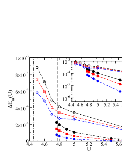
Figure 1: Absolute differences (13) between the SCPT and DMFT ground-state energies as functions of $U$ for the orders $m=9$ (circle), $m=11$ (square), and $m=15$ (diamond). Open and solid symbols correspond to DMRG-DMFT and QMC-DMFT, respectively. Vertical lines mark the critical coupling $U_{c}$ deduced from DMRG-DMFT (dot-dash) and QMC-DMFT (dash) studies. Other lines are guides for the eye. The inset shows the same data on a logarithmic scale.

Using the coefficients $a_{n}$ we can define the partial sums

$$E_{m}(U)=\sum_{n=0}^{m}\frac{a_{n}}{U^{n}}$$ (12)

which give the ground-state energy for a given Hubbard interaction $U$ and a given order of the SCPT up to $m=15$. Figure 1 shows the absolute differences

$$\Delta E_{m}(U)=\left|E_{\text{DMFT}}(U)-E_{m}(U)\right|$$ (13)

between the SCPT and DMFT ground-state energies for several $U$ and three different orders $m$. We see that $\Delta E_{m}(U)$ decreases for stronger interaction $U$ and higher order $m$, as expected. The energy differences are also systematically smaller for QMC-DMFT than for DMRG-DMFT, especially for larger $U$. However, this is easily explained by the different precision goal of these two distinct DMFT computations: DMRG energies [12] were calculated with an accuracy of $10^{-4}$ to $10^{-5}t$ while the QMC data [10] were recorded with an accuracy of $10^{-8}t$. Moreover, we see in Fig. 1 that the DMRG energy differences become significantly larger close to the critical value $U_{c}\approx 4.45$ determined in a DMRG-DMFT calculation. [12] This behavior is expected because the SCPT energies should become rapidly inaccurate as $U$ approaches the convergence radius of the perturbation series. Surprisingly, the QMC energy differences do not show any sign of a singularity close to the critical coupling $U_{c}\approx 4.78$ deduced from QMC-DMFT computations. [22] Therefore, the simple analysis of the energy differences $\Delta E_{m}(U)$ between SCPT and DMFT does not allow us to discriminate between both impurity solvers.

In principle, one can examine the convergence of the sequence of partial sums $\{E_{m}(U);m=1,3,5,\dots\}$ to determine the exact ground-state energy for any given $U>U_{c}$. In practice, the extrapolation of a finite number of available terms $E_{m}(U)$ to the limit $m\rightarrow\infty$ is often ambiguous. The case $U=4.8$ is particularly interesting. In Ref. 10 it was shown that the SCPT ground-state energies $E_{m}(U)$ up to $m=9$ could be well fitted with a quadratic function

$$E_{m}=E_{\infty}+c_{1}x+c_{2}x^{2}$$ (14)

with

$$x=\frac{2}{m+1}$$ (15)

and the three fit parameters $E_{\infty},c_{1},c_{2}$. The extrapolated value for $m\rightarrow\infty$ was found to be $E_{\infty}=-0.110259$ for $U=4.8$ in excellent agreement with the QMC-DMFT result $E_{\text{DMFT}}(U=4.8)=-0.11026919$. However, the choice of the scaling (15) is rather arbitrary. Indeed, in Ref. 12 it was shown that the same SCPT ground-state energies could be equally well fitted by a quadratic function (14) with

$$x=\frac{2}{m-1}.$$ (16)

The extrapolated value for $m\rightarrow\infty$ was then found to be $E_{\infty}=-0.110487$ in good agreement with the DMRG-DMFT result $E_{\text{DMFT}}(U=4.8)\approx-0.11048$. [It is not surprising that we cannot discriminate between the two possibilities (15) and (16) because we actually fit four data points $\{E_{m};m=3,5,7,9\}$ using four parameters if we also allow for the adjustment of the scaling of $x$ with $m$.] The same analysis was carried out using the 11–th order contribution calculated two years ago [11] but this additional term alone did not change the results significantly enough to discriminate between both fits.

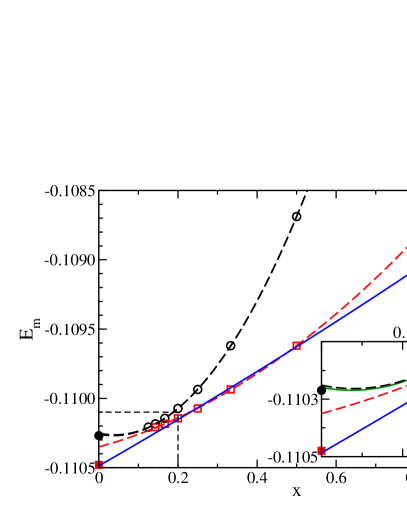
Figure 2: SCPT ground-state energy $E_{m}(U=4.8)$ as a function of $x=\frac{2}{m+1}$ (open circles) and $x=\frac{2}{m-1}$ (open squares). Lines represent least-square quadratic fits (14) of these data using all points ($m\leq 15$, black or red dashed lines) and all but the leftmost two points ($m\leq 11$, blue or green solid lines). The solid circle and square correspond to the QMC-DMFT and DMRG-DMFT results for $U=4.8$, respectively. The inset shows an expanded view of the box in the lower left corner.

Using the two additional contributions calculated in this work ($m=13$ and $15$) we find that the fit based on the first scaling (15) remains virtually unchanged from the result for $m\leq 11$, see Fig. 2. In particular, the extrapolated energy $E_{\infty}=-0.110252$ for $U=4.8$ is still in excellent agreement with the QMC-DMFT result. By contrast, Fig. 2 shows that the fitted parabola based on the second scaling (16) changes significantly if one uses all known data points $E_{m}$ ($m\leq 15$) or only the previously available ones ($m\leq 11$). The extrapolated energy $E_{\infty}=-0.110350$ now differs visibly from the DMRG-DMFT result and shifts closer to the QMC-DMFT result.

We have analyzed the SCPT convergence for various values of $U$ using a more general scaling $x=2/(m+w)$. All results confirm that the choice $w=1$ yields the most stable extrapolations (14) and that the extrapolated SCPT energies $E_{\infty}$ agree very well with the QMC-DMFT energies for $U\geq 4.8$. Moreover, they confirm that the agreement between SCPT and DMRG-DMFT energies deteriorates for $U\leq 5$ when the orders $n=13$ and $n=15$ are taken into account even if one chooses another parameter $w$. Therefore, we conclude that (15) is the best scaling for extrapolating ground-state energies and that the QMC-DMFT calculations [10] are more accurate than the DMRG-DMFT computations [12] in the critical region above $U_{c}$.

III.2 Extrapolated perturbation theory

Rather than extrapolating the ground-state energy for a given coupling $U$, we can use the Domb-Sykes method [38; 39] to conjecture the asymptotic behavior of the coefficients $a_{n}$. Thus we can obtain the critical behavior of the ground-state energy and also extrapolate the partial sums (12) to very high orders $m$. This approach was named extended perturbation theory (ePT) in previous works. [10; 11]

For odd $n\geq 3$ we define the number sequence

$$R_{n}=\sqrt{\frac{a_{n}}{a_{n-2}}}.$$ (17)

Assuming that the convergence radius $U_{R}$ of the series (10) is identical with the critical coupling $U_{c}$ where the Mott phase becomes unstable, the ratio criterion implies that

$$\lim_{n\rightarrow\infty}R_{n}=U_{c}.$$ (18)

To extrapolate the sequence for $n\rightarrow\infty$, one can again use a least-square quadratic fit

$$R_{n}=U_{c}+g_{1}x+g_{2}x^{2}$$ (19)

with $x=2/(n+w)$, and the three fit parameters $U_{c},g_{1},g_{2}$. The corresponding Domb-Sykes plots are shown in Fig. 3. If we assume that the singular part of the ground-state energy (4) for $U\lesssim U_{c}$ is a power law

$$E_{c}(U)\propto\left(U-U_{c}\right)^{\tau-1}$$ (20)

with a critical exponent $\tau\neq 1,2,3,\dots$, the coefficients of the series (5) must satisfy the asymptotic relation

$$R_{n}\approx U_{c}\left(1-\frac{\tau}{n}\right)$$ (21)

for $n\gg 1$. [38; 39; 48] Therefore, we can estimate the critical exponent from the fit parameters with

$$\tau=-\frac{2g_{1}}{U_{c}}.$$ (22)

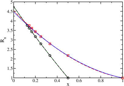
Figure 3: Domb-Sykes plot of the ratio $R_{n}$ as a function of $x=\frac{2}{m+1}$ (open circles) and $x=\frac{2}{m-1}$ (open squares). Lines represent quadratic least-square fits (19) of these data using all points ($m\leq 15$, black or red dashed lines) and all but the leftmost two points ($m\leq 11$, blue or green solid lines).

On the basis of the SCPT coefficients $a_{n}$ up to $n=9$, it was shown that $U_{c}\approx 4.75$ and $\tau\approx 3.44$ using $w=1$ [10] but $U_{c}\approx 4.43$ and $\tau\approx 2.61$ using $w=-1$ [12]. On the one hand, the former critical parameters agreed well with several DMFT calculations for $U_{c}$ [21; 22; 23; 10; 24] but none of these studies proposed a value for $\tau$. On the other hand, the latter critical parameters were in excellent agreement with the DMRG-DMFT results $U_{c}\approx 4.45$ and $\tau=5/2$. [12] Moreover, the value $U_{c}\approx 4.406$ was obtained from a perturbative solution of the DMFT self-consistency problem. [27] Including the 11-th order coefficient did not change the critical parameters significantly and hence did not solve the controversy. [11]

Using the two additional orders computed in this work, we find that the critical parameters are only insignificantly modified, $U_{c}\approx 4.76$ and $\tau\approx 3.45$, for the choice $w=1$. For $w=-1$, however, the fit parabola becomes visibly different for $x\rightarrow 0$, see Fig. 3, and the resulting critical parameters are now $U_{c}\approx 4.55$ and $\tau\approx 2.55$. While the change of $\tau$ is negligible (and the new value agrees rather better with the DMRG-DMFT $\tau=5/2$ than previously), the critical coupling $U_{c}$ shifts significantly away form the DMRG-DMFT result [12] toward the value obtained in other DMFT calculations. We have also probed other values of $w$ but clearly the choice $w=1$ yields the most stable extrapolation with respect to variations of the numbers of exact coefficients $a_{n}$. Therefore, we conclude that the critical parameters are $U_{c}\approx 4.76$ and $\tau\approx 3.45$ based on the 15-th order SCPT and the Domb-Sykes method.

Assuming that the relation (19) holds for all coefficients $R_{n}$ with $n>15$ we can compute the coefficients $a_{n}$ for $n>15$ recursively and thus extend the partial sum (12) to very high orders $m$. Additionally, as we know the asymptotic behavior of the coefficients

$$a_{n}=-U_{c}^{n}\frac{C}{n^{\tau}}$$ (23)

with a constant $C\approx 0.349$, we can easily estimate the cutoff $m$ for a given $U$ and accuracy goal. In Ref. 10, it was shown using this extrapolated perturbation series (and the exact coefficients up to $n=9$) that the resulting ground-state energies agree with the QMC-DMFT data within $10^{-5}t$. Using the additional exact coefficients $a_{n}$ up to $n=15$ and extrapolated ones up to $m=1001$, we find that the differences between the extrapolated perturbation series and the QMC-DMFT ground-state energies are now of the order of $10^{-7}t$ or smaller for all $U-U_{c}\geq 0.04$. Therefore, we have not only confirmed that the QMC-DMFT data are numerically exact (i.e., within their stated precision of $10^{-8}t$) but also that the extrapolated perturbation series can reach the same level of accuracy even very close to the critical coupling.

IV Conclusion and outlook

We have investigated the ground-state energy in the Mott insulating phase of the Hubbard model on a Bethe lattice with infinite coordination number using a combinatorial-diagrammatic approach based on the Kato-Takahashi strong-coupling perturbation theory. First, we have carried out large-scale computer-algebra calculations to obtain the exact coefficients $a_{n}$ of the series expansion (5) up to the 15-th order in $1/U$. Then, a Domb-Sykes analysis of the series asymptotic behavior has allowed us to determine its singular behavior close to the critical coupling $U_{c}$ below which the Mott phase becomes unstable. We have thus established highly accurate benchmarks for DMFT methods.

The DMFT method [3; 4] is a complex numerical technique and the result quality depends not only on the impurity solver used (e.g., DMRG, QMC or NRG) but also on the chosen discretization scheme for the continuous self-consistency equation. As DMRG is a very reliable method for quantum impurity problems and other DMRG-DMFT investigations [23; 24] agree with QMC-DMFT results, the failure of the DMRG-DMFT computation close to the critical coupling in Ref. 12 is probably due to the discretization scheme used in that work. Indeed, an essential step of this particular scheme is the deconvolution of the impurity density of states calculated with DMRG. In a recent work [49], two of us have shown that the deconvolution procedure used in Ref. 12 slightly distorts the shape of the density of states in a one-dimensional paramagnetic Mott-Hubbard insulator. We think that a similar deconvolution inaccuracy could be responsible for the failure of the DMRG-DMFT scheme in Ref. 12 .

The computer-algebra SCPT method presented in Sec. (II) can be extended to various generalizations of the Hubbard model (1). For instance, one could vary $t_{\downarrow}$ continuously to interpolate between the Hubbard model ($t_{\downarrow}/t_{\uparrow}=1$) and the Falicov-Kimball model ($t_{\downarrow}/t_{\uparrow}=0$) or one could study Hubbard models with several bands [50; 51] or internal $SU(n)$ symmetries with large $n$. [52; 53] Kato perturbation theory has already been applied to the Mott insulating phase in the strong-coupling limit of the Bose-Hubbard model with spinless bosons. [54; 55; 56] In that case, the unperturbated ground state is not degenerate and thus the perturbation series can easily be computed up to high orders. For bosons with spin $S>0$, however, the degeneracy of the unperturbated ground state duplicates the situation encountered in the Hubbard model for electrons. Thus, the approach that we have used for the fermionic Hubbard model can also be applied to a spin-disordered Mott phase in the Bose-Hubbard model with spin $S>0$ as well as to Mott phases of other fermion systems and of boson-fermion mixtures in optical lattices. [13; 14; 17]

However, an essential condition for the computer-algebra SCPT used in this work is the conservation of the singlet ground-state degeneracy at all orders in the series expansion, which allows one to evaluate the correlation functions (9) easily. If this property is not fulfilled, an exact calculation of the relevant correlation functions could become much more difficult or even impossible. Then one would have to be content with (possibly numerical) approximations for the coefficients $a_{n}$ of the perturbation series. Obviously, this degeneracy at finite coupling is a model property and thus the applicability of our method has to be checked on a case to case basis. The loss of degeneracy seems also to be the most serious difficulty in extending the combinatorial-diagrammatic approach to the Hubbard model away from half filling and, more generally, to metallic phases in the strong-coupling limit. Indeed, away from half filling the degeneracy of the $U=\infty$ ground state is already partially lifted in first order in the hopping term $T$. Again, this seems to imply that one could only obtain approximate series coefficients $a_{n}$ away from half filling. Similarly, we could employ the computer-algebra SCPT as an approximation method for the Hubbard model on other lattice geometries than the Bethe lattice and for finite dimensions or coordination numbers. (The DMFT method is already used as an approximative method for treating strong electronic correlations in finite dimensional systems, for instance, in first-principles studies of three-dimensional systems. [4; 19; 20])

One of the open problems in the theory of Mott insulators is the shape of the Hubbard bands in the single-particle density of states (DOS). In particular, DMFT calculations reveal some unexplained sharp structures at the low-energy edges of the Hubbard bands in both the Mott insulating phase [12] and the metallic phase [24; 57] in the critical region. The DOS of the Mott insulating phase has been calculated perturbatively up to the second order in $1/U$ directly from the Hubbard model [35] and up to the third order by solving the DMFT self-consistency equation [27]. However, these results do not fully explain the observed structures. Moreover, the DMFT results for the DOS depend sensitively on the scheme used to solve the self-consistent impurity problem [24]. In that case we are clearly in need of more accurate results, such as higher-order terms in the perturbation expansion.

In principle, the combinatorial-diagrammatic approach can be extended to the calculation of the local single-particle Green's function, which determines the DOS and the Mott-Hubbard gap. The series expansion can be formulated as a self-consistent integral equation for the Green's function at finite $U$. The equation contains polynomials of the Green's function at $U\rightarrow\infty$ with increasing orders. The coefficients of these polynomials can be calculated using a similar combinatorial-diagrammatic approach as the coefficients for the series expansion of the ground-state energy (5). However, the computational cost appears to be significantly higher for the Green's function than for the ground state series expansion. Moreover, it is not clear whether we can obtain an exact solution with combinatorial-diagrammatic techniques only, because methods from numerical analysis could be required to solve the self-consistent integral equation. Nevertheless, it would be worthwhile to calculate even only a few higher order contributions to the Green's function. Knowing higher-order contributions to DOS and gap would allow us to determine the critical coupling $U_{c}$ and the critical exponent $\tau$ more accurately and thus to gain a better understanding of the paramagnetic Mott metal-insulator transition. Moreover, this would provide us with a more direct and thorough benchmarking of numerical DMFT methods because they are actually based on self-consistent computations of the Green's function.

The development of the combinatorial-diagrammatic approach to the Kato-Takahashi SCPT has greatly benefited from a formal mathematical study of its algorithms. [45; 44] Discrete mathematics rather than differential calculus provides the mathematical background for this approach. Further development of similar computer-algebra perturbation methods will require a close cooperation between physics and discrete mathematics which will benefit both fields. Indeed, we have not only used the On-Line Encyclopedia of Integer Sequences (OEIS) [46] to obtain information on known integer sequences but also contributed new ones. For instance, the number of sequences $N_{s}$ in Table 1 is the integer sequence A198761 in OEIS.

The computer-algebra techniques developed in this work for large-scale computations of the Kato-Takahashi SCPT could also be applied to other series expansions. [28; 29; 30; 31] For instance, the method of continuous unitary transformations can be used to map the Hubbard model at strong coupling onto an effective model with conservation of the number of double occupancies [58; 59; 60]. Using appropriate truncation schemes one can close, and thus solve, the flow equations [61] of the effective Hamiltonians. This results in a systematic expansion of the effective Hamiltonian and other observables in powers of $1/U$, which is very similar to Kato perturbation expansion. One possible approach is a truncation of the equations in a perturbative manner to obtain a series expansion. [32] Recently, a non-perturbative approach has been proposed based on graph-theoretical methods. [33] Therefore, we think that larger-scale computer-algebra calculations will also prove useful for these approaches in the future.

- [1] T. Kato, Prog. Theor. Phys. 4, 514 (1949).
- [2] M. Takahashi, J. Phys. C 10, 1289 (1977).
- [3] D. Vollhardt, Ann. Phys. (Berlin) 524, 1 (2012).
- [4] D. Vollhardt, M. Kollar, and K. Byczuk, Dynamical Mean-Field Theory in A. Avella and F. Mancini (eds.), Strongly Correlated Systems (Springer Series in Solid-State Sciences 171, Berlin, 2012).
- [5] N. F. Mott, Metal-Insulator Transitions (Taylor and Francis, London, 1990).
- [6] F. Gebhard, The Mott Metal-Insulator Transition (Springer, Berlin, 1997).
- [7] J. Hubbard, Proc. R. Soc. A 276, 237 (1963).
- [8] M. C. Gutzwiller, Phys. Rev. Lett. 10, 159 (1963).
- [9] J. Kanamori, Prog. Theor. Phys. 30, 275 (1963).
- [10] N. Blümer and E. Kalinowski, Phys. Rev. B 71, 195102 (2005).
- [11] E. Kalinowski and W. Gluza, Phys. Rev. B 85, 045105 (2012).
- [12] S. Nishimoto, F. Gebhard, and E. Jeckelmann, J. Phys.: Condens. Matter 16, 7063 (2004).
- [13] M. P. A. Fisher, P. B. Weichman, G. Grinstein, and D. S. Fisher, Phys. Rev. B 40, 546 (1989).
- [14] E. Altman, E. Demler, and A. Rosch, Phys. Rev. Lett. 109, 235304 (2012).
- [15] Y. Kurosaki, Y. Shimizu, K. Miyagawa, K. Kanoda, and G. Saito, Phys. Rev. Lett. 95, 177001 (2005).
- [16] M. Greiner, O. Mandel, T. Esslinger, T. W. Hänsch, and I. Bloch, Nature 415, 39 (2002).
- [17] I. Bloch, J. Dalibard, and W. Zwerger, Rev. Mod. Phys. 80, 885 (2008).
- [18] P. G. J. van Dongen, Phys. Rev. B 45, 2267 (1992).
- [19] E. Pavarini, E. Koch, D. Vollhardt, A. Lichtenstein, editors, The LDA+DMFT approach to strongly correlated materials(Forschungszentrum Jülich, Jülich, 2011).
- [20] N. Lin, C. A. Marianetti, A. J. Millis, and D. R. Reichman, Phys. Rev. Lett. 106, 096402 (2011).
- [21] R. Bulla, T. A. Costi, and D. Vollhardt, Phys. Rev. B 64, 045103 (2001).
- [22] N. Blümer, PhD thesis, University of Augsburg, 2002; Mott-Hubbard Metal-Insulator Transition and Optical Conductivity in High Dimensions (Shaker Verlag, Aachen, 2003).
- [23] D. J. Garcia, K. Hallberg, and M. J. Rozenberg, Phys. Rev. Lett. 93, 246403 (2004).
- [24] M. Karski, C. Raas, and G. S. Uhrig, Phys. Rev. B 72, 113110 (2005); Phys. Rev. B 77, 075116 (2008).
- [25] F. Gebhard, E. Jeckelmann, S. Mahlert, S. Nishimoto, and R. M. Noack, Eur. Phys. J. B 36, 491 (2003).
- [26] E. Müller-Hartmann, Z. Phys. B – Condensed Matter 76, 211 (1989).
- [27] D. Ruhl and F. Gebhard, Phys. Rev. B 83, 035120 (2011).
- [28] J. Oitmaa, C. Hamer, and W. Zheng, Series Expansion Methods for Strongly Interacting Lattice Models (Cambridge University Press, Cambridge, 2006).
- [29] S. Sawatdiaree and W. Apel, Physica E 6, 75 (2000).
- [30] G. Hager, A. Weiße, G. Wellein, E. Jeckelmann, and H. Fehske, J. Magn. Magn. Mater. 310, 1380 (2007); Erratum 316, 43 (2007).
- [31] A. L. Chernyshev, D. Galanakis, P. Phillips, A. V. Rozhkov, and A.-M. S. Tremblay, Phys. Rev. B 70, 235111 (2004).
- [32] H. Y. Yang, A. M. Läuchli, F. Mila, and K. P. Schmidt, Phys. Rev. Lett. 105, 267204 (2010).
- [33] H. Y. Yang and K. P. Schmidt, Europhys. Lett. 94, 17004 (2011).
- [34] D. Klagges and K. P. Schmidt, Phys. Rev. Lett. 108, 230508 (2012).
- [35] M. P. Eastwood, F. Gebhard, E. Kalinowski, S. Nishimoto, and R. Noack, Eur. Phys. J. B 35, 155 (2003).
- [36] E. Kalinowski, PhD thesis, University of Marburg, 2002.
- [37] E. Kalinowski and F. Gebhard, J. Low Temp. Phys. 126, 979 (2002).
- [38] C. Domb and M. F. Sykes, Proc. R. Soc. A 240, 214 (1957).
- [39] C. Domb and M. F. Sykes, J. Math. Phys. 2, 63 (1961).
- [40] K. Schmidt (private communication).
- [41] J. C. Butcher, The Numerical Analysis of Ordinary Differential Equations (Wiley, Chichester, 1976).
- [42] T. Granlund and the GMP development team, [http://gmplib.org/].
- [43] D. E. Knuth, The Art of Computer Programming (Addison-Wesley Longman, Amsterdam, 2011).
- [44] G. Gruber, Diploma thesis, University of Marburg, 2012.
- [45] R. Loogen (private communication).
- [46] N. J. A. Sloane, The On-Line Encyclopedia of Integer Sequences, [http://oeis.org].
- [47] G. Hager and G. Wellein, Introduction to High Performance Computing for Scientists and Engineers (CRC Press, Boca Raton, 2011).
- [48] C. Hunter and B. Guerrieri, SIAM J. Appl. Math. 39, 248 (1980).
- [49] M. Paech and E. Jeckelmann, Phys. Rev. B 89, 195101 (2014).
- [50] E. Jakobi, N. Blümer, and P. van Dongen, Phys. Rev. B 80, 115109 (2009).
- [51] M. Greger, M. Kollar, and D. Vollhardt, Phys. Rev. Lett. 110, 046403 (2013).
- [52] L. Bonnes, K. R. A. Hazzard, S. R. Manmana, A. M. Rey, and S. Wessel, Phys. Rev. Lett. 109, 205305 (2012).
- [53] N. Blümer and E. V. Gorelik, Phys. Rev. 87, 085115 (2013).
- [54] N. Teichmann, D. Hinrichs, and M. Holthaus, and A. Eckardt, Phys. Rev. B 79, 100503 (2009); Phys. Rev. B 79, 224515 (2009).
- [55] A. Eckardt, Phys. Rev. B 79, 195131 (2009).
- [56] C. Heil and W. von der Linden, J. Phys.: Condens. Matter 24, 295601 (2012).
- [57] R. Zitko and T. Pruschke, Phys. Rev. B 79, 085106 (2009).
- [58] J. Stein, J. Stat. Phys. 88, 487 (1997).
- [59] A. Reischl, E. Müller-Hartmann, and G. S. Uhrig, Phys. Rev. B 70, 245124 (2004).
- [60] S. A. Hamerla, S. Duffe, and G. S. Uhrig, Phys. Rev. B 82, 235117 (2010).
- [61] S. Kehrein, The Flow Equation Approach to Many-Particle Systems (Springer, Berlin, 2006).