ICCUB-14-062

Unification of Coupling Constants, Dimension six Operators and the Spectral Action

Agostino Devastato^1,2, Fedele Lizzi^1,2,3, Carlos Valcárcel Flores⁴ and Dmitri Vassilevich⁴

¹Dipartimento di Fisica, Università di Napoli Federico II

²INFN, Sezione di Napoli
Monte S. Angelo, Via Cintia, 80126 Napoli, Italy

³ Departament de Estructura i Constituents de la Matèria,
Institut de Ciències del Cosmos, Universitat de Barcelona,
Barcelona, Catalonia, Spain

⁴ CMCC-Universidade Federal do ABC, Santo Andrè, S.P., Brazil

devastato@na.infn.it, fedele.lizzi@na.infn.it, valcarcel.flores@gmail.com, dvassil@gmail.com

We investigate whether inclusion of dimension six terms in the Standard Model lagrangean may cause the unification of the coupling constants at a scale comprised between $10^{14}$ and $10^{17}$ GeV. Particular choice of the dimension 6 couplings is motivated by the spectral action. Given the theoretical and phenomenological constraints, as well as recent data on the Higgs mass, we find that the unification is indeed possible, with a lower unification scale slightly favoured.

1 Introduction

The coupling constants of the three gauge interactions run with energy [1]. The ones relating to the nonabelian symmetries are relatively strong at low energy, but decrease, while the abelian interaction increases. At an energy comprised between $10^{13}-10^{17}$ GeV their values are very similar, around $0.52$, but, in view of present data, and in absence of new physics, they fail to meet at a single scale. Here by absence of new physics we mean extra terms in the Lagrangian of the model. The extra terms may be due for example to the presence of new particles, or new interaction. A possibility could be supersymmetric models which can alter the running and cause the presence of the unification point [2].

The standard model of particle interaction coupled with gravity may be explained to some extent as a particular for of Noncommutative, or spectral geometry, see for example [3] for a recent introduction. The principles of noncommutative geometry are rigid enough to restrict gauge groups and their fermionic representations, as well as to produce a lot of relations between bosonic couplings when applied on (almost) commutative spaces. All these restrictions and relations are surprisingly well compatible with the Standard Model, except that the Higgs field comes out too heavy, and that the unification point of gauge couplings is not exactly found. We have nothing new to say about the first problem, which has been solved in [4, 5, 6, 7, 8] with the introduction of a new scalar field $\sigma$ suitably coupled to the Higgs field, but we shall address the second one.

Some years ago the data were compatible with the presence of a single unification point $\Lambda$. This was one of the motivations behind the building of grand unified theories. Such a feature is however desirable even without the presence of a larger gauge symmetry group which breaks to the standard model with the usual mechanisms. In particular, the approach to field theory, based on noncommutative geometry and spectral physics [10], needs a scale to regularize the theory. In this respect, the finite mode regularization [11, 12, 13] is ideally suited. In this case $\Lambda$ is also the field theory cutoff. In fact using this regularization it is possible to generate the bosonic action starting form the fermionic one [14, 15, 16], or describe induced gravity on an equal footing with the anomaly-induced effective action [17]

The aim of this paper is to investigate whether the presence of higher dimensional terms in the standard model action $-$ dimension six in particular $-$ may cause the unification of the coupling constants. The paper may be read in two contexts: as an application of the spectral action, or independently on it, from a purely phenomenologically point of view.

From the spectral point of view, the spectral action [10] is solved as a heath kernel expansion in powers in the inverse of an energy scale. The terms up to dimension four reproduce the standard model qualitatively, but the theory is valid at a scale in which the couplings are equal. The expansion gives, however, also higher dimensional terms, suppressed by the power of the scale, and depending on the details of the cutoff. This fixes relations among the coefficients of the new terms. The analysis of this paper gives the conditions under which the spectral action can predict the unification of the three gauge coupling constants.

On the other side, it is also possible to read the paper at a purely phenomenological level, using the spectral action as input only for the choice of the subset of all possible higher dimensions terms in the action, and as a guide for the setting of the low energy values for the couplings of the coefficients of the extra terms. We show that the presence of these terms enables the possibility of a unification.

In both cases the scale of unification $\Lambda$ is considered the cutoff, and we run the theory below it. We assume, therefore, that perturbation theory is valid. There appears a hierarchy problem. From the point of view of the spectral action this implies a rather strange (though admissible) cutoff function. From a phenomenological point of view this entails either unnaturally large dimensionless quantities, or the presence of a new intermediate scale, $\Gamma$. The latter option is, of course, more desirable and we will discuss it below.

The paper is organized as follows: in section 2, we present the action of Standard Model (SM) of particle physics, and the standard running coupling constants. We show how the spectral action approach $-$ whose principles are summarized in the appendix A $-$ fits the SM. In section 3 we give the new renormalization group equations at one loop, due to the dimensions-6 operators; then, we show how these new operators affect the SM phenomenology. In section 4 we run the renormalization group equations to study the new coupling constants behavior, checking the possibility to improve the gauge unification point. A final section contains conclusions and some comments and open questions.

2 Standard Model Running Coupling Constans

The standard model action (including right handed neutrinos) is:

$$\mathcal{L}_{SM} = -\frac{1}{4}V_{\mu\nu}^{A}V^{A\mu\nu}-\frac{1}{4}W_{\mu\nu}^{I}W^{I\mu\nu}-\frac{1}{4}B_{\mu\nu}B^{\mu\nu}+\left(D_{\mu}H\right)^{\dagger}D^{\mu}H-\frac{m^{2}}{2}H^{\dagger}H-\lambda\left(H^{\dagger}H\right)^{2}+$$ (2.1)

$$-\left(\overline{e}\mathbf{F}_{L}H^{\dagger}l+\overline{d}\mathbf{F}_{D}H^{\dagger}q+\overline{u}\mathbf{F}_{U}H^{c\dagger}q+h.c.\right)+\mbox{Majorana mass terms}$$

where $B_{\mu\nu}$, $W_{\mu\nu}^{I}$ and $V_{\mu\nu}^{A}$ are respectively the field strengths associated with the gauge groups $U(1),\,SU(2)$ and $SU(3)$; the gauge covariant derivative is $D_{\mu}=\partial_{\mu}+ig_{3}T^{A}A_{\mu}^{A}+ig_{2}t^{I}W_{\mu}^{I}+ig_{1}\mbox{y}B_{\mu}$, where $T^{A}$ are the $SU(3)$ generators, $t^{I}=\tau^{I}/2$ are the $SU(2)$ generators, and y is the $U(1)$ hypercharge generator. $H$ is the Higgs field, a $SU(2)$ scalar doublet with hypercharge $1/2$ and its charged conjugated field defined as $H^{c}\equiv i\tau_{2}H^{*}$. The three families of fermions are grouped together so that $\mathbf{F}_{L}$, $\mathbf{F}_{U}$, $\mathbf{F}_{D}$ are the $3\times 3$ complex Yukawa matrices acting on the hidden flavor index of every fermion field. Since these matrices are dominated by the Yukawa coupling $y_{t}$ of the top quark, in the following we will consider this parameter only. Likewise we will consider a single mass term for the Majorana masses: $y_{\nu}$.

This Lagrangian can be obtained from first principles using the spectral action [18, 19], which is a regularized trace, with $\Lambda$ appearing as the cutoff. We give the details of the spectral action calculations in the appendix. For the economy of this paper the relevant part is the fact that the spectral action requires the coupling constants of the three gauge groups to be equal at a scale $\Lambda$, which is also the cutoff of the theory. There is no need for a unified gauge group at the scale $\Lambda$, which in fact may signify a phase transition to a pre geometric phase [20], although larger symmetries are also possible [5, 7]. As explained in the appendix, the spectral action is an expansion in inverse powers of $\Lambda^{2}$, and it enables the presence of a set of new dimension six operators. Dimension five operators, which violate lepton number, and do not change the properties of the Higgs boson are not present in the expansion. The spectral action also gives relations among the coefficients of the required dimension six operators, which are described in detail in the appendix A. The reader interested only in the phenomenological aspect of this paper may skip the appendix, and accept our choice of operator as a convenient one.

A complete classification of the dimension-six operators in the standard model is given in [21]. There it is shown that there are 59 independent operators, preserving baryon number, after eliminating redundant operators using the equations of motion. Here we consider only the following dimension-six operators, mixing the gauge field strength and the Higgs field. They are the ones coming from the spectral action expansion:

$$\mathcal{L}^{(6)} = C_{HB}H\overline{H\,}B_{\mu\nu}B^{\mu\nu}+C_{HW}H\overline{H}\,\mathbf{W}_{\mu\nu}\mathbf{W}^{\mu\nu}+C_{HV}H\overline{H}\,\mathbf{V}_{\mu\nu}\mathbf{V}^{\mu\nu}+$$ (2.2)

$$+C_{W}\mathbf{W}_{\mu\nu}\mathbf{W}^{\nu\alpha}\mathbf{W}_{\alpha}^{\mu}+C_{V}\mathbf{V}_{\mu\nu}\mathbf{V}^{\nu\alpha}\mathbf{V}_{\alpha}^{\mu}+C_{H}\left(\overline{H}H\right)^{3}$$

The coefficients $C$ have the dimension of an inverse energy square. The spectral action fixes their value at the cutoff $\Lambda$. To these terms we have to add a coupling between the Higgs, the $W$ and the $B$ which is absent in the spectral action at scale $\Lambda$, but is dynamically created. With the couplings considered here no other term is induced.

The SM running coupling constants at one loop, associated to (2.1), are ruled by the following equations, where we defined the dot derivations as $16\pi^{2}\mu\frac{d}{d\mu}$:

$$\dot{g}_{i} = \left(b_{i}g_{i}^{3}\right)\,\,\mbox{with}\,\left(b_{1},b_{2},b_{3}=\frac{41}{6},-\frac{19}{6},-7\right)$$

$$\dot{\lambda} = \left(24\lambda^{2}-\left(3g_{1}^{2}+9g_{2}^{2}\right)\lambda+\frac{3}{8}\left(g_{1}^{4}+2g_{1}^{2}g_{2}^{2}+3g_{2}^{4}\right)+\left(12y_{t}^{2}+4y_{\nu}^{2}\right)\lambda-6y_{t}^{4}-2y_{\nu}^{4}\right)$$

$$\dot{y}_{t} = \left(\frac{9}{2}y_{t}^{2}+y_{\nu}^{2}-\frac{17}{12}g_{1}^{2}-\frac{9}{4}g_{2}^{2}-8g_{3}^{2}\right)$$

$$\dot{y}_{\nu} = \left(\frac{5}{2}y_{\nu}^{2}+3y_{t}^{2}-\frac{3}{4}g_{1}^{2}-\frac{9}{4}g_{2}^{2}\right)$$ (2.3)

For the purposes of this paper one loop is sufficient, the running up to three loops can be found in [22, 23, 24, 25] and references therein. In the present case, one separately solves the equations for the gauge coupling constants and the other couplings; for the former, the boundary conditions are given at the electro-weak scale by the experimental values [1],

$$g_{1}(m_{Z})=0.358,\,\,g_{2}(m_{Z})=0.651,\,\,g_{3}(m_{Z})=1.221\,$$ (2.4)

while for the other coupling constants $\lambda,y_{t}$ and $y_{\nu}$ the boundary conditions are taken at the cut-off scale $\Lambda$ that is the scale at which the spectral action lives. These boundary conditions use the parameters of the fermions that are the inputs in the Dirac operator (A.2), as shown in the appendix A,

$$\lambda(\Lambda) =\frac{4\left(\rho^{2}+3\right)}{\left(\rho+3\right)^{2}}g^{2}$$

$$y_{t}(\Lambda) =\sqrt{\frac{4}{\rho^{2}+3}}g$$

$$y_{\nu}(\Lambda) =\sqrt{\frac{4\rho^{2}}{\rho^{2}+3}}g$$ (2.5)

$\rho$ is a free parameter such that $y_{\nu}(\Lambda)=\rho\,y_{t}(\Lambda)$ and $g\equiv g_{3}(\Lambda)=g_{2}(\Lambda)=\frac{5}{3}g_{1}(\Lambda)$. Since the coupling constants $g_{i}$ do not meet exactly, forming a triangle, one takes for $\Lambda$ a range of values beetwen the extremal points of the triangle. The results, for a particular set of values of the parameters $(g,\rho,\Lambda)=(0.530,\,1.25,10^{16}GeV)$, are plotted in Fig. 1.

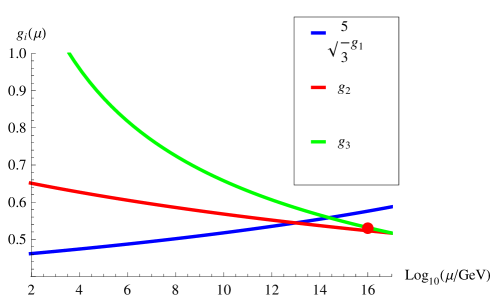
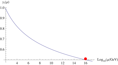
Figure 1: The standard model running for the gauge coupling constant (left) and the Yukawa coupling (right) in the spectral action approach for $(g,\rho,\Lambda)=(0.530,\,1.25,\,10^{16}GeV)$. The red dot indicates the starting value of the parameters (Log${}_{10}(\frac{\Lambda}{GeV}),g$) and (Log${}_{10}(\frac{\Lambda}{GeV}),\lambda(\Lambda)$).

After running these couplings from unification energy $\Lambda$ to low energy $M_{Z}$, we compare the values of $y_{t}(M_{Z})$ and $\lambda(M_{Z})$ with their experimental values

$$y^{exp}_{t}(M_{Z})=0.997,\,\,\ \lambda^{exp}(M_{Z})=0.130$$ (2.6)

In Fig. 1 we can see the good agreement between $y_{t}(M_{Z})$ predicted by the spectral action and its experimental value. Very different is the case for the Higgs self-coupling $\lambda$, Fig. 2, whose predicted value, in the spectral action approach, is around 0.240 with a resulting Higgs mass $M_{H}=\sqrt{2\lambda v^{2}}\simeq 170$  GeV. On the other hand, the experimental value for the Higgs mass ($\simeq$125 GeV) leads to the instability problem for the self-interaction parameter $\lambda$, which becomes negative at a scale of the order of $10^{8}GeV$; two loop calculations make the situation slightly worse as one can see on the left side of Fig. 2.

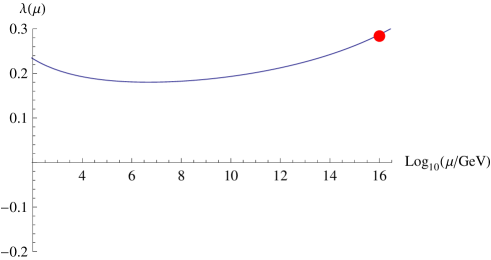
Figure 2: On the left, the standard model running for the coupling constant $\lambda$ starting from $\lambda(m_{Z})=0.130$ corresponding to $M_{H}=125GeV$. The dashed and solid lines represent the one and two loop respectively. On the right, the $\lambda$ behaviour starting from the red point of the spectral action and culminating in the prediction $\lambda(m_{Z})=0.240$.

A negative $\lambda$ means an instability and renders the model inconsistent, although it may just mean the presence of a long lived metastable state [26, 27]. The spectral action model can be fixed [4, 5, 6, 7, 8] with the introduction of a scalar field, $\sigma$, possibly coming from a larger symmetry, connected with the fluctuations of a Majorana neutrino mass term in the action. Since the running of the Higgs parameters do not affect strongly the running of the coupling constants (which are the true aim of this paper), nor does this field $\sigma$, we will not consider it in what follows. However, a more complete and accurate analysis will necessitate also this element, and it is in progress. Also the presence of gravitational couplings in the spectral action could alter significativly the running at high energy leading to an asymptotically free theory at the Planck scale [9].

3 Coupling Constants RGEs

In this section we give the new renormalization group equations (RGEs) at one loop due to the dimensions-6 operators in the Lagrangian (2.2). Although the choice of the dimension six operators and some of characteristics of the Lagrangian are coming from the spectral action, this section can be read independently of it.

The full one-loop contributions to the SM running for dimension six operators have been calculated in [28, 29, 30, 31]. The modifications to the standard model RGEs are given by the following new terms to be added to the rhs of (2.3):

$$\delta\dot{g_{3}} = -4m_{H}^{2}g_{3}C_{HV}$$

$$\delta\dot{g_{2}} = -4m_{H}^{2}g_{2}C_{HW}$$

$$\delta\dot{g_{1}} = -4m_{H}^{2}g_{1}C_{HB}$$

$$\delta\dot{\lambda}\ = m_{H}^{2}\left(9g_{2}^{2}C_{HW}+3g_{1}^{2}C_{HB}+12C_{H}+3g_{1}g_{2}C_{HWB}\right)$$

$$\delta\dot{y}_{t,\nu} = 0$$ (3.1)

and the RGEs for the dim-6 coupling constants are given by

$$\dot{C}_{HB} =C_{HB}\left(12\lambda+2\left(3y_{t}^{2}+y_{\nu}^{2}\right)+\frac{85}{6}g_{1}^{2}-\frac{9}{2}g_{2}^{2}\right)+3C_{HWB}g_{1}g_{2}$$

$$\dot{C}_{HW} =C_{HW}\left(12\lambda+2\left(3y_{t}^{2}+y_{\nu}^{2}\right)-\frac{47}{6}g_{1}^{2}-\frac{5}{2}g_{2}^{2}\right)+C_{HWB}g_{1}g_{2}-15C_{W}g_{2}^{3}$$

$$\dot{C}_{HV} =C_{HV}\left(12\lambda+2\left(3y_{t}^{2}+y_{\nu}^{2}\right)-\frac{3}{2}g_{1}^{2}-\frac{9}{2}g_{2}^{2}-14g_{3}^{2}\right)$$

$$\dot{C}_{HWB} =C_{HWB}\left(4\lambda+2\left(3y_{t}^{2}+y_{\nu}^{2}\right)+\frac{19}{3}g_{1}^{2}+\frac{4}{3}g_{2}^{2}\right)+2g_{1}g_{2}\left(C_{HB}+C_{HW}\right)+3C_{W}g_{1}g_{2}^{2}$$

$$\dot{C}_{W} =\frac{29}{2}C_{W}g_{2}^{2}$$

$$\dot{C}_{V} =15C_{V}g_{3}^{2}$$

$$\dot{C}_{H} =C_{H}\left(108\lambda+6\left(3y_{t}^{2}+y_{\nu}^{2}\right)-\frac{9}{2}g_{1}^{2}-\frac{27}{2}g_{2}^{2}\right)-3C_{B}g_{1}^{2}\left(g_{1}^{2}+g_{2}^{2}-4\lambda\right)+$$

$$\,\,\,\,+3C_{W}g_{2}^{2}\left(12\lambda-3g_{2}^{2}-g_{1}^{2}\right)+C_{HWB}\left(12\lambda g_{1}g_{2}-3g_{1}^{3}g_{2}-3g_{1}g_{2}^{3}\right)$$ (3.2)

Although the spectral action does not contain explicitly the term $C_{HWB}H^{2}W_{\mu\nu}B^{\mu\nu}$, due to the unimodular condition, the coupling constant $C_{HWB}$ is however induced by the running of $C_{HB},\,C_{HW}$ and $C_{W}$.

In the framework of the spectral action these equations are solved with boundary conditions at the cut-off scale $\Lambda$ given by the coefficients appearing in (A.44):

$$C_{HB}(\Lambda) =-\frac{f_{6}}{16\pi^{2}\Lambda^{2}}\frac{4\left(3\rho^{2}+17\right)}{9\left(\rho^{2}+3\right)}g^{4}\,\,,\,C_{HW}(\Lambda)=-\frac{f_{6}}{16\pi^{2}\Lambda^{2}}\frac{4}{3}g^{4}\,\,,\,C_{HV}(\Lambda)=-\frac{f_{6}}{16\pi^{2}\Lambda^{2}}\frac{16}{3\left(\rho^{2}+3\right)}g^{4}\,\,,$$

$$C_{H}(\Lambda) =-\frac{f_{6}}{16\pi^{2}\Lambda^{2}}\frac{512(\rho^{6}+3)}{3\left(\rho^{2}+3\right)^{3}}g^{6}\,\,,\,\,\,\,\,C_{W}(\Lambda)=-\frac{f_{6}}{16\pi^{2}\Lambda^{2}}\frac{26}{15}g^{3}\,\,,\,\,\,\,\,C_{V}(\Lambda)=-\frac{f_{6}}{16\pi^{2}\Lambda^{2}}\frac{26}{15}g^{3}\,.\,\,\,$$ (3.3)

The coupling $C_{HWB}$ is set to zero at the cut-off scale $C_{HWB}(\Lambda)=0$ since it does not appear in the spectral action.

In (3.3) $g\equiv g_{3}(\Lambda)=g_{2}(\Lambda)=\frac{5}{3}g_{1}(\Lambda)$ is the value of the gauge coupling constants at the cut-off scale which, therefore, is identified with the unification scale. These two constants, $g$ and $\Lambda$, together with the ratio $\rho$ and the parameter $f_{6}$ appearing in the spectral action, will be the four free parameters of this model.

There are also constraints at low energy to satisfy. The values of the $g_{i}$’s are known at the scale of the top mass with very high precision, and the parameters $\lambda$ and the $y_{t}$ are related to the Higgs and top mass. As we said earlier, the spectral action requires a positive value of $\lambda$ at the cutoff scale $\Lambda$, (2.5), and without the field $\sigma$, it predicts a mass of the Higgs at 170 GeV. However, the presence of higher-order operators in the action alters the form of the usual coupling constants, leading to a new phenomenology which we outline in the following section.

3.1 New phenomenology

In this section, following [31, sect.5] we give the main modifications to the SM phenomenology due to the dim-6 Lagrangian, i.e. the new form of the observables measured at the electroweak scale. The new operators, in fact, alter the definition of the SM parameters at tree level in several ways.

First of all, we focus on the effects of the dimension-six Lagrangian on the Higgs mass $m_{H}$ and the self-coupling $\lambda$. The dim-6 operator $C_{H}\bar{H}H$ changes the shape of the scalar doublet potential at order $C_{H}v^{2}$ to

$$V(H)=-\frac{m^{2}}{2}H^{\dagger}H+\lambda\left(H^{\dagger}H\right)^{2}-C_{H}\left(H^{\dagger}H\right)^{3}$$ (3.4)

generating the new minimum

$$\left\langle H^{\dagger}H\right\rangle = \frac{1}{3C_{H}}\left(\lambda-\sqrt{\lambda^{2}-3C_{H}\lambda v^{2}}\right)$$ (3.5)

$$\simeq \frac{v^{2}}{2}\left(1+\frac{3C_{H}v^{2}}{4\lambda}\right)\equiv\frac{v_{T}^{2}}{2}$$

in the second line we have expanded the exact solution to first order in $C_{H}.$ Therefore the shift in the vacuum expectation value is proportional to $C_{H}v^{2},$ which is of order $f_{6}\frac{v^{2}}{\Lambda^{2}}.$ On expanding the potential (3.4) around the minimum and neglecting kinetics corrections,

$$H=\frac{1}{\sqrt{2}}\left(\begin{array}[]{c}0\\ h+v_{T}\end{array}\right),$$ (3.6)

we find for the Higgs boson mass

$$m_{H}^{2}=2\lambda v_{T}^{2}\left(1-\frac{3C_{H}v^{2}}{2\lambda}\right)$$ (3.7)

At the same time the gauge fields and the gauge couplings are also affected by the dim-6 couplings.

In the broken theory the $X^{2}H^{2}$ operators (with $X$ being any field strength) contribute to the gauge kinetic energies, through the Lagrangian terms

$$\left(\mathcal{L}_{SM}+\mathcal{L}_{6}\right)_{kin} = -\frac{1}{4}B_{\mu\nu}B^{\mu\nu}-\frac{1}{4}G_{\mu\nu}G^{\mu\nu}-\frac{1}{4}W_{\mu\nu}^{3}W_{3}^{\mu\nu}-\frac{1}{2}W_{\mu\nu}^{+}W_{-}^{\mu\nu}+$$

$$+\frac{1}{2}v_{T}^{2}\left(C_{HB}B_{\mu\nu}B^{\mu\nu}+C_{HW}W_{\mu\nu}W^{\mu\nu}+C_{HG}G_{\mu\nu}G^{\mu\nu}-C_{HWB}W_{\mu\nu}^{3}B^{\mu\nu}\right)$$

while for the mass terms of the gauge bosons, arising from $(D_{\mu}H)^{\dagger}(D^{\mu}H$), we have

$$\left(\mathcal{L}_{SM}+\mathcal{L}_{6}\right)_{mass}=\frac{1}{4}g_{2}^{2}v_{T}^{2}W_{\mu\nu}^{+}W_{-}^{\mu\nu}+\frac{1}{8}v_{T}^{2}\left(g_{2}W_{\mu}^{3}-g_{1}B_{\mu}\right)^{2}+\frac{1}{16}v_{T}^{4}C_{HD}\left(g_{2}W_{\mu}^{3}-g_{1}B_{\mu}\right)^{2}$$ (3.9)

The gauge fields have to be redefined, so that the kinetic terms are properly normalized and diagonal,

$$G_{\mu}=\mathcal{G}_{\mu}\left(1+C_{HG}v_{T}^{2}\right),\,\,W_{\mu}=\mathcal{W}_{\mu}\left(1+C_{HW}v_{T}^{2}\right),\,\,B_{\mu}=\mathcal{B}_{\mu}\left(1+C_{HB}v_{T}^{2}\right),$$ (3.10)

so that the modified coupling constants become

$$\bar{g}_{3}=g_{3}\left(1+C_{HG}v_{T}^{2}\right),\,\,\bar{g}_{2}=g_{2}\left(1+C_{HW}v_{T}^{2}\right),\,\,\bar{g}_{1}=g_{1}\left(1+C_{HB}v_{T}^{2}\right),$$ (3.11)

and the products $g_{1}B_{\mu}=\bar{g}_{1}\mathcal{B}_{\mu}$ etc. are unchanged. Therefore, the electroweak Lagrangian is

$$\mathcal{L} = -\frac{1}{4}\mathcal{B}_{\mu\nu}\mathcal{B}^{\mu\nu}-\frac{1}{4}\mathcal{W}_{\mu\nu}^{3}\mathcal{W}_{3}^{\mu\nu}-\frac{1}{2}\mathcal{W}_{\mu\nu}^{+}\mathcal{W}_{-}^{\mu\nu}-\frac{1}{2}\left(v_{T}^{2}C_{HWB}\right)\mathcal{W}_{\mu\nu}^{3}\mathcal{B}^{\mu\nu}$$ (3.12)

$$+\frac{1}{4}\bar{g}_{2}^{2}v_{T}^{2}\mathcal{W}_{\mu\nu}^{+}\mathcal{W}_{-}^{\mu\nu}+\frac{1}{8}v_{T}^{2}\left(\bar{g}_{2}\mathcal{W}_{\mu}^{3}-\bar{g}_{1}\mathcal{B}_{\mu}\right)^{2}+\frac{1}{16}v_{T}^{4}C_{HD}\left(\bar{g}_{2}\mathcal{W}_{\mu}^{3}-\bar{g}_{1}\mathcal{B}_{\mu}\right)^{2}.$$

The mass eigenstate basis is given by, [31, eq.5.21],

$$\left[\begin{array}[]{c}\mathcal{W}_{\mu}^{3}\\ \mathcal{B}_{\mu}\end{array}\right]=\left[\begin{array}[]{cc}1&-\frac{1}{2}v_{T}^{2}C_{HWB}\\ -\frac{1}{2}v_{T}^{2}C_{HWB}&1\end{array}\right]\left[\begin{array}[]{cc}\mbox{cos}\bar{\theta}&\mbox{sin}\bar{\theta}\\ \mbox{-sin}\bar{\theta}&\mbox{cos}\bar{\theta}\end{array}\right]\left[\begin{array}[]{c}\mathcal{Z}_{\mu}^{3}\\ \mathcal{A}_{\mu}\end{array}\right],$$ (3.13)

with $\bar{\theta}$, rotation angle, given by

$$\mbox{tan}\bar{\theta}=\frac{\bar{g}_{1}}{\bar{g}_{2}}+\frac{v_{T}^{2}}{2}C_{HWB}\left[1-\frac{\bar{g}_{1}^{2}}{\bar{g}_{2}^{2}}\right]\,.$$ (3.14)

The photon remains massless and the $W$ and $Z$ masses are

$$M_{W}^{2} = \frac{\bar{g}_{2}^{2}v_{T}^{2}}{4},$$

$$M_{Z}^{2} = \frac{(\bar{g}_{1}^{2}+\bar{g}_{2}^{2})v_{T}^{2}}{4}+\frac{1}{8}v_{T}^{4}C_{HD}\left(\bar{g}_{1}^{2}+\bar{g}_{2}^{2}\right)+\frac{1}{2}v_{T}^{4}\bar{g}_{1}\bar{g}_{2}C_{HWB}$$ (3.15)

The covariant derivative has the form

$$D_{\mu}=\partial_{\mu}+i\frac{\bar{g}_{2}}{\sqrt{2}}\left[\mathcal{W}_{\mu}^{+}T^{+}+\mathcal{W}_{\mu}^{-}T^{-}\right]+ig_{Z}\left[T_{3}-\mbox{sin}\bar{\theta}^{2}Q\right]\mathcal{Z}_{\mu}+i\bar{e}Q\mathcal{A}_{\mu},$$ (3.16)

where $Q=T_{3}+Y$ and the effective couplings become,

$$\bar{e} = \frac{\bar{g}_{1}\bar{g}_{2}}{\sqrt{\bar{g}_{1}^{2}+\bar{g}_{2}^{2}}}\left[1-\frac{\bar{g}_{1}\bar{g}_{2}}{\bar{g}_{1}^{2}+\bar{g}_{2}^{2}}v_{T}^{2}C_{HWB}\right]=\bar{g}_{2}\mbox{sin}\bar{\theta}-\frac{1}{2}\mbox{cos}\bar{\theta}\bar{g}_{2}v_{T}^{2}C_{HWB}\,,$$

$$\bar{g}_{Z} = \sqrt{\bar{g}_{1}^{2}+\bar{g}_{2}^{2}}+\frac{\bar{g}_{1}\bar{g}_{2}}{\sqrt{\bar{g}_{1}^{2}+\bar{g}_{2}^{2}}}v_{T}^{2}C_{HWB}=\frac{\bar{e}}{\mbox{sin}\bar{\theta}\mbox{cos}\bar{\theta}}\left[1+\frac{\bar{g}_{1}^{2}+\bar{g}_{2}^{2}}{2\bar{g}_{1}\bar{g}_{2}}v_{T}^{2}C_{HWB}\right]\,,$$

$$\mbox{sin}\bar{\theta}^{2} = \frac{\bar{g}_{1}^{2}}{\bar{g}_{1}^{2}+\bar{g}_{2}^{2}}+\frac{\bar{g}_{1}\bar{g}_{2}\left(\bar{g}_{2}^{2}-\bar{g}_{1}^{2}\right)}{\bar{g}_{1}^{2}+\bar{g}_{2}^{2}}v_{T}^{2}C_{HWB}\,.$$ (3.17)

Considering (3.17) and (3.15), the experimental values for the $W$ and $Z$ masses and couplings fix $\bar{g}_{1},$$\bar{g}_{2},$$v_{T}$, $C_{HWB}$ and $C_{HD}.$ This procedure consists of solving 5 equations in 5 variables: the unique solution of this system is given by the classical values for $\bar{g}_{1},$$\bar{g}_{2}$ and $v_{T}$, i.e.

$$\bar{g}_{1}=0.358,\,\,\bar{g}_{2}=0.651,\,\,v_{T}=246\,GeV$$ (3.18)

while the dim-6 parameters $C_{HWB}$ and $C_{HD}$ have to give negligble corrections to the standard results. This means the products $v_{T}^{2}C_{HWB}$ and $v_{T}^{2}C_{HD}$ have to be, at least, of the order $10^{-3}$, i.e. $C_{HWB,D}\lesssim 10^{-7}GeV^{-2}$.

4 Running of the constants

In the following section we run the renormalization group equations, presented in sect. 3, to study the modification of the coupling constants behavior, due to the dim-6 operators. We check the possibility, for these new terms, to give a gauge unification point and to return values for the coupling constants compatible with the spectral action predictions.

4.1 Renormalization group flow

One can run the equations of the renormalization group in two directions. A “bottom-up” running assumes boundary values for the various constants at low energy (usually the $Z$ or top mass) and runs toward higher energies. This is the way Fig. 1 has been obtained. On the contrary the spectral action is defined at the high energy scale $\Lambda$, and its strength lies in the fact that it specifies the boundary conditions of all constants there. Therefore a “top-down” approach is more natural. In this paper we follow a combined approach.

We start at the scale $\Lambda$ in the range $10^{13-17}$ GeV. At this energy we give the boundary values given by the spectral action. In particular we use for the dimension six terms the values we have calculated and presented in (3.3). The top-down running depends on four other parameters (described below) and gives a set of values for all of physical parameters at low energy. The parameters we find are not too distinct from the experimentally known ones, but there are discrepancies. As it should be: the heat kernel expansion is akin to a one loop calculation and, apart form any other incomplete aspect of the theory, it would be unreasonable to find the correct values for all parameters. The values one finds are however close to the experimental ones for the three $g_{i}$ and $y_{t}$, while as remarked earlier $\lambda$, which is the parameter appearing in the Higgs mass, is off by nearly a factor two. The top-down running gives a set of values of the dimension six couplings $C_{i}$ at $M_{Z}$ .

We then performed a bottom-up running to see if the presence of the new terms could give a unification point, and we found that in several cases it does. As boundary conditions we used the experimental values for the $g_{i}$’s and $y_{t}$ and the low energy values of the $C_{i}$’s obtained in the top-down running. The case of $\lambda$ deserves a little discussion. Since the experimental and spectral action values are quite different, the qualitative behaviour in the two cases are different. On the other side, it is known that the problem is fixed by the presence of another field ($\sigma$), which we do not discuss in this paper. We have therefore performed our analysis in the two cases, i.e. the value of $\lambda$ obtained by the spectral action, and the experimental one. The strategy we followed is synthesized in Table 1.

$$\left[\begin{array}[]{ccc}\Lambda\ \mbox{scale}\overset{\mbox{\small RGEs}}{\longrightarrow}M_{Z}\,\mbox{scale}&&M_{Z}\,\mbox{scale}\overset{\mbox{\small RGEs}}{\longrightarrow}\Lambda\mbox{scale}\\ \mbox{\small In:}\{\mbox{\small eq.(\ref{eq: constrains new})}\}&&\mbox{\small In:}\{C_{i}(M_{Z}),\,g_{i}^{exp}\}\\ \mbox{\small Out:}\{\mbox{\small}C_{i}(M_{Z})\}&&\mbox{\small Out:}\{C_{i}(\Lambda),g_{i}(\Lambda)\}\\ \underbrace{\,\,\,\,\,\,\,\,\,\,\,\,\,\,\,\,\,\,\,\,\,\,\,\,\,\,\,\,\,\,\,\,\,\,\,\,\,\,\,\,\,\,\,\,\,\,\,\,\,\,\,\,\,\,\,\,\,\,}&&\underbrace{\,\,\,\,\,\,\,\,\,\,\,\,\,\,\,\,\,\,\,\,\,\,\,\,\,\,\,\,\,\,\,\,\,\,\,\,\,\,\,\,\,\,\,\,\,\,\,\,\,\,\,\,\,\,\,\,\,\,}\\ {\color[rgb]{0,0,1}\mbox{top-down\,\ running}}&&{\color[rgb]{0,0,1}\mbox{bottom-up\,\ running}}\end{array}\right]$$ (4.1)

Table 1: Resolution scheme adopted for the renormalization group flow. Varying $\Lambda,\,g,\,\rho$ and $f_{6}$ we solve the RGEs, starting from the unification scale $\Lambda$ down to the $M_{Z}$ scale, and we use the resulting values for the dim-6 parameters together with the experimental values for the usual dim-4 couplings $g_{i}^{exp},\,\lambda^{exp},\,y_{top}^{exp}$ to run again toward high energies.

The second case, in which we used the experimental values as initial conditions, can be considered on a purely phenomenological basis, to show that higher dimension operators may cause unifications of the constants at one loop.

4.2 Top-Down running

In the spectral action model we have four free parameters: the value of the gauge coupling constants at the unification, $g$. The value of the cut-off and unification scale, $\Lambda$. The ratio between top and neutrino Yukawa couplings, $\rho$. The momentum $f_{6}$ which will fix the new physics scale $\Gamma$. This last parameter appears as coefficient to the dimension six operators with the combination $f_{6}/\Lambda^{2}$, and therefore effectively defines a new energy scale.

All parameters have a particular range in which we expect they could be chosen. From the SM running of the gauge coupling constants we know $g$ is expected around $0.55\pm 0.03$, while $\Lambda$ has a more significant range between $10^{13}$ GeV and $10^{17}$ GeV. The ratio $\rho$ between the top and neutrino Yukawa couplings should be expected of $O(1)$. The value of the parameter $f_{6}$ requires a separate discussion. From the internal logic of the spectral action its “natural” value would be of order unity, or not much larger. Such a value would however make the corrections to the running totally irrelevant. The parameter appears with a denominator in $\Lambda^{2}$, and the corrections are often quadratic in this ratio. On the other side, from the phenomenology of electroweak processes it can be expected the effects of these new physics terms on the measured signal strength for $H\rightarrow\mathrm{\gamma\gamma}$ decay, whose measured value is given by ATLAS and CMS [32, 33]. To obtain comparable data the new physics scale has to be fixed around $\Gamma\thicksim 1-10$ TeV. This leads to expected values for the dim-6 coefficients $C_{i}$ around $10^{-6}-10^{-8}\mbox{GeV}^{-2}$ . The range for $f_{6}$ will be $\thicksim\Lambda^{2}/\Gamma^{2}$, i.e. $10^{20-28}$. Given the fact that the cutoff function is undetermined in the scheme, such numbers are allowed, although a more physical explanation of their size would be preferable. The spectral action, given by an expansion valid below the unification scale, gives a framework to use a perturbative expansion valid beyond the scale of new physics, although it does not explain it. From the spectral point of view this is a weak point, the presence of such a high value for $f_{6}$ is very strange and creates an unnatural hierarchy with the other coefficients.

Since the point of the calculation was to verify the possibility of unification, the top-down calculation has been performed with the aim of obtaining values which would be a good starting point for the bottom up calculation. We did search for the best solutions for the range of parameters above. We performed first a coarse search to restrict the range, and then optimized the input parameters to find a good unification point. For the scope of this paper, i.e. to show that dimension six operators could give unification, this is sufficient.

The boundary conditions at $M_{Z}$ for the subsequent bottom-up run approach are the experimental values for the $g_{i}$ and $y_{t}$, and the values obtained from the top-down for the $C_{i}$’s. In the case of $\lambda$ we have the two choices: either the values obtained from the top down, or the one from experiment. Since these two are different, in the following we present both cases.

4.2.1 Spectral action value for $\lambda$

In the following table we describe the values of the free parameters we used which will enable the best unification.

Table 2 shows, for various values of $\Lambda$, the parameters used for the top-down running, and the value of the couplings at low energy, shown as ratio with respect to the experimental value, corrected as described in the previous section: $\gamma_{i}=\frac{g_{i}(M_{Z})}{\bar{g}^{exp}_{i}}$ and $\gamma_{t}=\frac{y_{t}(M_{Z})}{y_{t}^{exp}}$. The values for $\lambda$ are not shown since, for the reasons described above, they are not significant.

$\Lambda$ GeV	$g(\Lambda)$	$\rho(\Lambda)$	$\frac{f_{6}}{16\pi^{2}\Lambda^{2}}\mbox{Gev}^{-2}$	$\gamma_{1}$	$\gamma_{2}$	$\gamma_{3}$	$\gamma_{t}$
$10^{14}$	0.580	1.6	$4.8~{}10^{-6}$	$1.0$	$1.0$	$1.0$	$1.0$
$10^{15}$	0.570	1.9	$7.3~{}10^{-6}$	$0.98$	$1.0$	$1.0$	$1.0$
$10^{16}$	0.550	1.9	$6.9~{}10^{-6}$	$0.95$	$0.99$	$1.0$	$1.0$
$10^{17}$	0.540	2.0	$8.3~{}10^{-6}$	$0.93$	$0.97$	$1.1$	$1.0$

Table 2: The values of the coupling constants at $M_{Z}$ compared with the experimental values for the top-down running. The values of the free parameters are optimized for the subsequent bottom-up run.

Note that the choice of parameters has been made to optimize the subsequent bottom-up running. The amount of variations with respect to the experimental values for the couplings could be made smaller with a different choice of $g,f_{6}$ and $\rho$. This top-down running gives values for the $C_{i}$’s, which are shown in Table 3.

$\Lambda$	$C_{HWB}$	$C_{W}$	$C_{V}$	$C_{HV}$	$C_{H}$	$C_{HB}$	$C_{HW}$
$10^{14}$	$1.1\,10^{-7}$	$-5.8\,10^{-7}$	$-2.7\,10^{-7}$	$-1.1\,10^{-6}$	$3.8\,10^{-8}$	$-1.7\,10^{-7}$	$-7.5\,10^{-7}$
$10^{15}$	$1.4\,10^{-7}$	$-8.1\,10^{-7}$	$-3.3\,10^{-7}$	$-1.4\,10^{-6}$	$5.6\,10^{-8}$	$-2.1\,10^{-7}$	$-9.9\,10^{-7}$
$10^{16}$	$1.2\,10^{-7}$	$-6.7\,10^{-7}$	$-2.6\,10^{-7}$	$-1.3\,10^{-6}$	$4.2\,10^{-8}$	$-1.7\,10^{-7}$	$-8.2\,10^{-7}$
$10^{17}$	$1.3\,10^{-7}$	$-7.4\,10^{-7}$	$-2.5\,10^{-7}$	$-1.4\,10^{-6}$	$4.6\,10^{-8}$	$-1.7\,10^{-7}$	$-8.8\,10^{-7}$

Table 3: The values of the coefficients of the dimension six operators at $M_{Z}$ . The values of the free parameters are the ones in Table 2. All $C_{i}$’s are in GeV^-2.

One can see that with the choice of parameters, mainly $f_{6}$, the $C_{i}$’s are in the range expected by a new physics scale of the order of 1 TeV.

4.2.2 Experimental value for $\lambda$

The values described above are made with parameters which are natural in the framework of the spectral action, but from the phenomenological point of view, since we now have the mass of the Higgs, and therefore the value of $\lambda(M_{Z})$, we can also perform the analysis using as boundary condition the experimental value. As in the previous subsection the parameters are chosen in such a way to optimize the subsequent bottom-up run. Tables 4 and 5 are the counterparts of 2 and 3 for the case optimized for unification using as input the experimental value of $\lambda$ at $M_{Z}$. Of course some principle like the spectral action must be operating in the background, to make sense of the fact that we are running the theory above the scale $\Gamma$ all the way to the unification point.

$\Lambda$ GeV	$g(\Lambda)$	$\rho(\Lambda)$	$\frac{f_{6}}{16\pi^{2}\Lambda^{2}}\mbox{Gev}^{-2}$	$\gamma_{1}$	$\gamma_{2}$	$\gamma_{3}$	$\gamma_{t}$
$10^{14}$	0.580	1.1	$1.1~{}10^{-5}$	$0.98$	$0.95$	$0.80$	$1.0$
$10^{15}$	0.560	0.7	$8.3~{}10^{-6}$	$0.98$	$0.96$	$0.85$	$1.1$
$10^{16}$	0.550	1.0	$9.6~{}10^{-6}$	$0.98$	$0.96$	$0.89$	$1.1$
$10^{17}$	0.540	0.9	$8.3~{}10^{-6}$	$0.99$	$0.98$	$0.95$	$1.2$

Table 4: The values of the coupling constants at $M_{Z}$ compared with the experimental values for the top-down running. The values of the free parameters are optimized for the subsequent bottom-up run. The initial value of $\lambda(M_{Z})$ is the experimental one.

One can see that with respect to the previous case the values of the $\gamma$’s are slightly worse, showing that in this case the result of the top-down running spectral action “predictions” are off. This is not surprising because for the subsequent running (for which these values are optimized) the connections with the spectral action are weaker.

$\Lambda$	$C_{HWB}$	$C_{W}$	$C_{V}$	$C_{HV}$	$C_{H}$	$C_{HB}$	$C_{HW}$
$10^{14}$	$2.3\,10^{-7}$	$-1.4\,10^{-6}$	$-7.3\,10^{-7}$	$-2.9\,10^{-6}$	$9.4\,10^{-8}$	$-4.4\,10^{-7}$	$-1.6\,10^{-6}$
$10^{15}$	$1.5\,10^{-7}$	$-9.0\,10^{-7}$	$-4.5\,10^{-7}$	$-2.4\,10^{-6}$	$6.1\,10^{-8}$	$-5.7\,10^{-8}$	$-1.3\,10^{-6}$
$10^{16}$	$1.6\,10^{-7}$	$-9.3\,10^{-7}$	$-4.0\,10^{-7}$	$-2.6\,10^{-6}$	$6.1\,10^{-8}$	$3.7\,10^{-7}$	$-1.1\,10^{-6}$
$10^{17}$	$1.3\,10^{-7}$	$-7.3\,10^{-7}$	$-2.6\,10^{-7}$	$-3.1\,10^{-6}$	$4.9\,10^{-8}$	$8.6\,10^{-7}$	$-8.6\,10^{-7}$

Table 5: The values of the coefficients of the dimension six operators at $M_{Z}$. The values of the free parameters are the ones in Table 2. All $C_{i}$’s are in GeV^-2.

One can notice that the values for the couplings in the two cases are not drastically different.

4.3 Bottom-up running

In this section we present the result of the running from low to high energy, with the parameters chosen to have the three coupling constants meet near a common value in the range $10^{14}-10^{17}$ GeV. As in the previous subsection we first discuss the case in which the boundary condition for $\lambda$ is the one obtained from the running of the spectral action.

4.3.1 Spectral action value for $\lambda$

A good solution is one for which the common intersection is the starting point for the top-down running, and the $C_{i}$ come back to the original values given by the spectral action. We optimized our search for the unification, therefore the fact that the values of the $C_{i}$ “come back” to the same order within a factor of two or so, and are not off by an order a magnitude, is a check. The coefficient $C_{HWB}$ is not present at the $\Lambda$ scale in the spectral action, in this case one should expect it to be smaller than the other. A further check is the value of the top Yukawa at $\Lambda$ which should be close to the value determined by the spectral action. The results for the coupling constants are in Table 6. The quantities $\delta g_{i}(\%)$ indicate (in percent) how different is the value of the runned constants ($g_{i}^{run})$ with respect to the original spectral action value $g(\Lambda)$ we started with, as shown in Table 2.

$$\delta g_{i}\%=\frac{|g_{i}^{run}(\Lambda-g(\Lambda)|}{g(\Lambda)}\times 100$$ (4.2)

with an analogous definition for $\delta y_{t}$.

$\Lambda$	$\delta g_{1}\%$	$\delta g_{2}\%$	$\delta g_{3}\%$	$\delta y_{t}\%$	$\delta\lambda\%$
$10^{14}$	1.4	2.1	0.17	0.30	4.1
$10^{15}$	3.3	0.02	0.54	3.6	4.7
$10^{16}$	7.8	0.078	0.97	6.4	2.3
$10^{17}$	13	1.7	1.1	6.6	3.9

Table 6: The percent variation of the values of the three coupling constants and the top Yukawa coupling compared with the initial values of the top-down run.

One can see that for the smaller values of $\Lambda\simeq 10^{14}-10^{15}$, one finds a good unification point, while for higher values the unification is worse. This can also be seen in Figs. 3 and 4 for the two extreme cases of $10^{14}$ and $10^{17}$ respectively, compared with the standard model running.

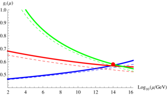
Figure 3: Running of the self-interaction parameter $\lambda$(on the rigth) and gauge coupling constants (on the left) in the presence of dimension six operators (thick lines) and their standard behaviour (dashed lines) for $\Lambda=10^{14}$GeV. The values of the parameters are discussed in the text. The red dot indicates the starting value of the parameter. The dashed lines are the values of the $g_{i}$’s in the standard model.

In the first case there is a good unification, while in the second case the point at which the constants meet is some way off the initial energy.

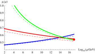
Figure 4: Same as in Fig. 3 for $\Lambda=10^{17}$GeV.

The values of the $C_{i}$’s at the scale $\Lambda$ are usually close to the one we started with in the top-down running, checking the consistency of the model. In particular $C_{HWB}$, which was zero, is constantly about one order of magnitude smaller than the other. We show this in Table 7 for the two extreme values of $\Lambda$.

$\Lambda=10^{14}$	$C_{HWB}$	$C_{W}$	$C_{V}$	$C_{HV}$	$C_{H}$	$C_{HB}$	$C_{HW}$
Spec. Act.	$0$	$-3.0\,10^{-6}$	$-3.0\,10^{-6}$	$-5.2\,10^{-7}$	$-3.7\,10^{-6}$	$-8.1\,10^{-7}$	$-7.3\,10^{-7}$
Run	$1.3\,10^{-8}$	$-1.5\,10^{-6}$	$-1.6\,10^{-6}$	$-5.5\,10^{-7}$	$-6.8\,10^{-6}$	$-6.7\,10^{-7}$	$-9.2\,10^{-7}$
$\Lambda=10^{17}$	$C_{HWB}$	$C_{W}$	$C_{V}$	$C_{HV}$	$C_{H}$	$C_{HB}$	$C_{HW}$
Spec. Act.	$0$	$-4.2\,10^{-6}$	$-4.2\,10^{-6}$	$-5.4\,10^{-7}$	$6.9\,10^{-6}$	$-1.0\,10^{-6}$	$-9.4\,10^{-7}$
Run	$5.0\,10^{-8}$	$-2.4\,10^{-6}$	$-1.9\,10^{-6}$	$-6.5\,10^{-7}$	$7.5\,10^{-6}$	$-8.7\,10^{-7}$	$-7.2\,10^{-7}$

Table 7: Comparison of the values of the coefficients of the dimension six operators at $\Lambda$. The second and fifth line are the initial values of the top-down running, as predicted by the spectral action for $\Lambda=10^{14}$. The third and the last lines refer to the $10^{17}$ case. All $C_{i}$’s are in GeV^-2.

Also in this case, the lower value for $\Lambda$ fares slightly better.

4.3.2 Experimental value for $\lambda$

If one ignores the spectral action, and trusts it only in that it gives some boundary values for the dimension six operator coefficients, then the bottom-up running can be performed independently. In this subsection we present, therefore, the running of the coupling constants using as boundary conditions at $M_{Z}$ the experimental values for the $g_{i}$, $y_{t}$, $\lambda$, (eq.2.4, 2.6), and the values of Table 5 for $C_{i}$’s and we check if the unification is possible. As we can see from Fig. 5,

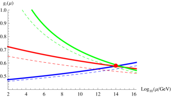
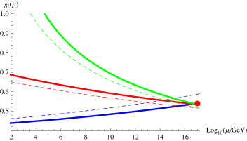
Figure 5: Gauge couplings unification for two different unification scale $\Lambda=10^{14}$GeV (left) and $\Lambda=10^{17}$GeV (right) if one relaxes the spectral action boundaries.

for two different unification scales, the answer is positive if one relaxes the values of the dim-6 coefficients with respect to that suggested by the spectral action. In fact, in this case, the value of the $\gamma$’s are slightly different from 1, as shown in table 4, but these allow to correct the unification point within an error of 1%, as summarized in Table 8.

$\Lambda(GeV)$	$\delta g_{1}\%$	$\delta g_{2}\%$	$\delta g_{3}\%$
$10^{14}$	0.62	0.74	1.0
$10^{15}$	1.4	0.38	0.56
$10^{16}$	1.2	0.50	0.50
$10^{17}$	0.14	0.98	1.1

Table 8: The percent variation of the values of the there coupling constants compared with the initial value of the unification point.

5 Conclusions and Outlook

In this paper we have calculated the sixth order terms appearing in the spectral action Lagrangian. We have then verified that the presence of these terms, with a proper choice of the free parameters, could cause the unification of the three constants at a high energy scale. Although the motivation for this investigation lies in the spectral noncommutative geometry approach to the standard model, the result can be read independently on it, showing that if the current Lagrangian describes an effective theory valid below the unification point, then the dimension six operator would play the proper role of facilitating the unification. In order for the new terms to have an effect it is however necessary to introduce a scale of the order of the TeV, which for the spectral action results in a very large second momentum of the cutoff function.

We note that we did not require a modification of the standard model spectral triple, although such a modification, and in particular the presence of the scale field $\sigma$, could actually improve the analysis. From the spectral action point of view the next challenge is to include the ideas currently come form the extensions of the standard model currently being investigated. From the purely phenomenological side instead a further analysis of the effects of the dimension six operators for phenomenaology at large, using the parameters suggested by this paper, can be a useful pointer to new physics.

Acknowledgements We thank Giancarlo D’Ambrosio and Giulia Ricciardi for discussions. DV was supported in parts by FAPESP, CNPq and by the INFN through the Fondi FAI Guppo IV Mirella Russo 2013. F.L. is partially supported by CUR Generalitat de Catalunya under projects FPA2013-46570 and 2014 SGR 104. A.D. and F.L. were partially supported by UniNA and Compagnia di San Paolo under the grant Programma STAR 2013. C.V.F. is supported by FAPESP.

Appendix A Spectral geometry

Noncommutative geometry is a way to describe noncommutative as well as commutative space on equal footing. Being quite general, this approach happens to be sufficiently rigid to make predictions about the standard model. Noncommutative geometry uses many tools of spectral geometry.

Generally, the geometry of a noncommutative space is defined through a Spectral Triple $\left(\mathcal{A},\mathcal{H},D\right)$ consisting of an algebra $\mathcal{A}$, a Hilbert space $\mathcal{H}$ and a Dirac operator $D$.

The algebra $\mathcal{A}$ should be thought of as a generalization of the algebra of functions to the case when the underlying space is possibly noncommutative. The noncommutative algebra $\mathcal{A}$ relevant for the standard model is the product of the ordinary algebra of functions on $\mathbb{R}^{4}$ times a finite dimensional matrix algebra $\mathcal{A}_{sm}=\mathbb{C}\oplus{\mathbb{H}}\oplus M_{3}(\mathbb{C})$. Here $\mathbb{H}$ is the algebra of quaternions, $M_{3}(\mathbb{C})$ is the algebra of complex $3\times 3$ matrices. $\mathcal{A}_{sm}$ may be interpreted as an algebra of functions on a finite ”internal” space. Since just the internal part $\mathcal{A}_{sm}$ is noncommutative, the geometry corresponding to Standard Model is called almost commutative. The gauge group is the group of automorphisms of $\mathcal{A}_{sm}$.

The algebra $\mathcal{A}$ acts on the Hilbert space $\mathcal{H}$. We take $\mathcal{H}=L^{2}(\mathrm{sp}(\mathbb{R}^{4}))\otimes\mathcal{H}_{F}$ being a tensor product of the space of square-integrable spinors and a finite-dimensional space $\mathcal{H}_{F}$. The algebra $\mathcal{A}_{sm}$ acts on $\mathcal{H}_{F}$, and this imposes severe restrictions on possible representations of the gauge group. Remarkably, these restrictions are satisfied by the Standard Model fermions. To incorporate all of these fermions one takes $\mathcal{H}_{F}=\mathcal{H}_{R}\oplus\mathcal{H}_{L}\oplus\mathcal{H}^{c}_{R}\oplus\mathcal{H}^{c}_{L}\oplus$, being $\mathcal{H}_{R}=\mathbb{C}^{24}$ ($8$ fermions with $3$ generations) the space of the right fermion, $\mathcal{H}_{L}=\mathbb{C}^{24}$ the space of the left fermions and the super index $c$ denotes their respectives antifermions. This give us the total of the $96$ SM degrees of freedom.

The Dirac operator $D$ also has to satisfy some consistency requirements, that all are respected in the Standard Model. These conditions

$$[\gamma,a]=0,\,\,\,\,[a,JbJ^{-1}]=0,\,\,\,\,[[D,a],JbJ^{-1}]=0$$ (A.1)

include the chirality operator $\gamma$ and the real structure $J$. Specifically, for the Standard Model the Dirac operator has the form

$$D=D_{M}\otimes 1_{96}+\gamma^{5}\otimes D_{F},$$ (A.2)

where $D_{M}=\gamma^{\mu}(\partial_{\mu}+\omega_{\mu})$ is the canonical Dirac operator and the chirality and real structure are $\gamma=\gamma^{5}\otimes\gamma_{F}$, $J=\mathcal{J}\otimes J_{F}$, with $\mathcal{J}$ being the charge conjugation. The finite dimensional Dirac operator $D_{F}$ is a matrix including the Yukawa couplings of leptons, Dirac and Majorana neutrinos. To introduce he gauge fields and the Higgs we replace $D$ by

$$D_{A}=D+\mathbb{A}+J\mathbb{A}J^{-1},$$ (A.3)

where $\mathbb{A}=\sum a[D,b]$, with $a,b\in\mathcal{A}$. In contrast to the usual Standard Model, the Noncommutative Standard Model includes a singlet scalar field $\sigma$. Roughly speaking, this field is a result of ”fluctuating” Majorana mass term of the Dirac operator and is responsible for adjusting the Higgs’ mass of noncommutative spectral action to the experimental values. Some other approaches to the Higgs mass problem in spectral action can be found in [4, 5, 7].

Following Chamseddine and Connes tensorial notation [19], an element $\Psi_{M}$ of the Hilbert space $\mathcal{H}$ is denoted as

$$\Psi_{M}=\left(\begin{array}[]{c}\psi_{\alpha I}\\ \psi_{\alpha^{\prime}I^{\prime}}\end{array}\right).$$ (A.6)

First, the primed indices denote the conjugate spinor, this is $\psi_{\alpha^{\prime}I^{\prime}}=\psi^{c}_{\alpha I}$. The index $\alpha$ acts on $\mathbb{C}\oplus\mathbb{H}$ and is decomposed as $\alpha=\dot{a},a$ where $\dot{a}=\dot{1},\dot{2}$ acts on $\mathbb{C}$ and $a=1,2$ acts on $\mathbb{H}$. The index $I$ acts on $\mathbb{C}\oplus M_{3}(\mathbb{C})$ and is decomposed as $I=1,i\,$: the index $1$ acts on $\mathbb{C}$, that is another copy of the algebra of complex numbers, and $i$ acts on $M_{3}(\mathbb{C})$.

Next, let us consider the action principle. One cannot construct too many invariants by using the spectral triple data. One obvious choice is the ordinary fermionic action

$$S_{F}=\langle\psi,D_{A}\psi\rangle\,.$$ (A.7)

As well, one can use the operator trace ${\rm Tr}$ in $\mathcal{H}$ to construct invariants from the Dirac operator alone. In this way one obtains the Spectral action

$$S_{\Lambda}\left(D\right)={\rm Tr}\,\left[f\left(\frac{D^{2}}{\Lambda^{2}}\right)\right],$$ (A.8)

where $f$ is a function restricted only by the requirement that trace in (A.8) exists. $f$ is usually called the cutoff function since it has to regularize (A.8) at large eigenvalues of $D$. $\Lambda$ is a cutoff scale.

One can use the heat kernel expansion

$${\rm Tr}\,\left[e^{-tD^{2}}\right]\simeq\sum_{p=0}^{\infty}t^{-2+p}a_{2p}\bigl{(}D^{2}\bigr{)}\,,\qquad t\to+0,$$ (A.9)

to find a large $\Lambda$ expansion of the Spectral Action. Suppose that $f$ is a Laplace transform,

$$f(z)=\int_{0}^{\infty}dt\,e^{-tz}\tilde{f}(t)\,.$$ (A.10)

Then

$$S_{\Lambda}\left(D\right)\sim\sum_{p=0}\Lambda^{4-2p}f_{2p}a_{2p}\left(D^{2}\right),$$ (A.11)

where

$$f_{2p}=\int_{0}^{\infty}dt\,t^{-2+p}\tilde{f}\left(t\right).$$ (A.12)

Note, that we have restricted ourselves to four dimensions where the first four terms of the asymptotic expansion are

$$S_{\Lambda}\left(D\right)\sim\Lambda^{4}f_{0}a_{0}\left(D^{2}\right)+\Lambda^{2}f_{2}a_{2}\left(D^{2}\right)+f_{4}a_{4}\left(D^{2}\right)+\frac{1}{\Lambda^{2}}f_{6}a_{6}\left(D^{2}\right)+\dots$$ (A.13)

$D^{2}$ is an operator of Laplace type. It can be represented as

$$D^{2}=-(\nabla^{2}+E)\,,$$ (A.14)

where $\nabla$ is a covariant derivative, $\nabla_{\mu}=\partial_{\mu}+\omega_{\mu}$, $E$ is a zeroth order term. Denoting by $\rm tr$ the usual matrix trace one may write

$$a_{0} = \frac{1}{16\pi^{2}}\int d^{4}x\sqrt{g}{\rm tr}\,\left(1\right),$$

$$a_{2} = \frac{1}{16\pi^{2}}\frac{1}{6}\int d^{4}x\sqrt{g}{\rm tr}\,\left[6E+R\cdot 1\right],$$

$$a_{4} = \frac{1}{16\pi^{2}}\frac{1}{360}\int d^{4}x\sqrt{g}{\rm tr}\,\left[\left(12R;_{\mu}^{\mu}+5R^{2}-2R_{\mu\nu}R^{\mu\nu}+2R_{\mu\nu\varrho\sigma}R^{\mu\nu\varrho\sigma}\right)\cdot 1\right]$$ (A.15)

$$+ \frac{1}{16\pi^{2}}\frac{1}{360}\int d^{4}x\sqrt{g}{\rm tr}\,\left[60E;_{\mu}^{\mu}+60ER+180E^{2}+30\Omega_{\mu\nu}\Omega^{\mu\nu}\right].$$ (A.16)

Here $R_{\mu\nu\rho\sigma}$, $R_{\mu\nu}$ and $R$ are the Riemann tensor, the Ricci tensor and the curvature scalar, respectively. The semicolon denotes covariant derivatives, and $\Omega_{\mu\nu}=\partial_{\mu}\omega_{\nu}-\partial_{\nu}\omega_{\mu}+[\omega_{\mu},\omega_{\nu}]$.

The expression for $a_{6}$ is rather long (see [35]), but it simplifies if one considers a flat-space time

$$a_{6}^{flat}=\frac{1}{16\pi^{2}}\int d^{4}x\left(\Sigma_{\Omega}+\Sigma_{E}+\Sigma_{E\Omega}\right),$$ (A.17)

where

$$\Sigma_{\Omega} = {\rm tr}\,\left[-\frac{1}{90}\Omega_{\mu\nu;\tau}\Omega^{\mu\nu;\tau}+\frac{1}{180}\Omega_{\;\;\;\;;\nu}^{\mu\nu}\Omega_{\mu\rho}^{\;\;\;\;;\rho}-\frac{1}{30}\Omega_{\mu\nu}\Omega^{\nu\tau}\Omega_{\tau}^{\;\;\mu}\right],$$ (A.18)

$$\Sigma_{E\Omega} = {\rm tr}\,\left[\frac{1}{12}E\Omega_{\mu\nu}\Omega^{\mu\nu}\right],$$ (A.19)

$$\Sigma_{E} = {\rm tr}\,\left[-\frac{1}{12}E^{;\mu}E_{;\mu}+\frac{1}{6}E^{3}\right],$$ (A.20)

Using the notation introduced in (A.6), the matrix elements of the connection $\omega_{\mu}$ are given by

$$\left(\omega_{\mu}\right)_{\dot{1}1}^{\dot{1}1} = 0,$$

$$\left(\omega_{\mu}\right)_{\dot{2}1}^{\dot{2}1} = ig_{1}B_{\mu}\otimes 1_{4}\otimes 1_{3},$$

$$\left(\omega_{\mu}\right)_{b1}^{a1} = i\left(\frac{g_{1}}{2}B_{\mu}\delta_{b}^{a}-\frac{g_{2}}{2}W_{\mu}^{\tau}\left(\sigma^{\tau}\right)_{b}^{a}\right)\otimes 1_{4}\otimes 1_{3},$$

$$\left(\omega_{\mu}\right)_{\dot{1}j}^{\dot{1}i} = i\left(-\frac{2g_{1}}{3}B_{\mu}\delta_{j}^{i}-\frac{g_{3}}{2}V_{\mu}^{m}\left(\lambda^{m}\right)_{j}^{i}\right)\otimes 1_{4}\otimes 1_{3},$$

$$\left(\omega_{\mu}\right)_{\dot{2}j}^{\dot{2}i} = i\left(\frac{g_{1}}{3}B_{\mu}\delta_{j}^{i}-\frac{g_{3}}{2}V_{\mu}^{m}\left(\lambda^{m}\right)_{j}^{i}\right)\otimes 1_{4}\otimes 1_{3},$$

$$\left(\omega_{\mu}\right)_{bj}^{ai} = i\left(-\frac{g_{1}}{6}B_{\mu}\delta_{b}^{a}\delta_{j}^{i}-\frac{g_{2}}{2}W_{\mu}^{\tau}\left(\sigma^{\tau}\right)_{b}^{a}\delta_{j}^{i}-\frac{g_{3}}{2}V_{\mu}^{m}\left(\lambda^{m}\right)_{j}^{i}\delta_{b}^{a}\right)\otimes 1_{4}\otimes 1_{3}.$$ (A.21)

Therefore, the components of the curvature $\Omega_{\mu\nu}$ are

$$\left(\Omega_{\mu\nu}\right)_{\dot{1}1}^{\dot{1}1} = 0,$$

$$\left(\Omega_{\mu\nu}\right)_{\dot{2}1}^{\dot{2}1} = ig_{1}B_{\mu\nu}\otimes 1_{4}\otimes 1_{3},$$

$$\left(\Omega_{\mu\nu}\right)_{b1}^{a1} = i\left(\frac{g_{1}}{2}B_{\mu\nu}\delta_{b}^{a}-\frac{g_{2}}{2}W_{\mu\nu}^{\tau}\left(\sigma^{\tau}\right)_{b}^{a}\right)\otimes 1_{4}\otimes 1_{3},$$

$$\left(\Omega_{\mu\nu}\right)_{\dot{1}j}^{\dot{1}i} = i\left(-\frac{2g_{1}}{3}B_{\mu\nu}\delta_{j}^{i}-\frac{g_{3}}{2}V_{\mu\nu}^{m}\left(\lambda^{m}\right)_{j}^{i}\right)\otimes 1_{4}\otimes 1_{3},$$

$$\left(\Omega_{\mu\nu}\right)_{\dot{2}j}^{\dot{2}i} = i\left(\frac{g_{1}}{3}B_{\mu\nu}\delta_{j}^{i}-\frac{g_{3}}{2}V_{\mu\nu}^{m}\left(\lambda^{m}\right)_{j}^{i}\right)\otimes 1_{4}\otimes 1_{3},$$

$$\left(\Omega_{\mu\nu}\right)_{bj}^{ai} = i\left(-\frac{g_{1}}{6}B_{\mu\nu}\delta_{b}^{a}\delta_{j}^{i}-\frac{g_{2}}{2}W_{\mu\nu}^{\tau}\left(\sigma^{\tau}\right)_{b}^{a}\delta_{j}^{i}-\frac{g_{3}}{2}V_{\mu\nu}^{m}\left(\lambda^{m}\right)_{j}^{i}\delta_{b}^{a}\right)\otimes 1_{4}\otimes 1_{3}.$$ (A.22)

The quantity $E$, which is defined through the operator $D^{2}$, has diagonal and non-diagonal components. The diagonal terms, i.e., $E_{\dot{1}1}^{\dot{1}1},E_{\dot{2}1}^{\dot{2}1},E_{b1}^{a1}$ and $E_{\dot{1}j}^{\dot{1}i},E_{\dot{2}j}^{\dot{2}i},E_{bj}^{ai}$ have the form $E^{\rm diag}=-\frac{1}{2}\gamma^{\mu\nu}\Omega_{\mu\nu}-U\otimes 1_{4}$, where

$$U_{\dot{1}1}^{\dot{1}1} = \left(\left|y_{\nu}\right|^{2}\overline{H}H+\left|y_{\nu_{R}}\right|^{2}\sigma^{2}\right),$$

$$U_{\dot{2}1}^{\dot{2}1} = \left(\left|y_{e}\right|^{2}\overline{H}H\right),$$ (A.23)

$$U_{b1}^{a1} = \left(\left|y_{e}\right|^{2}H_{a}\overline{H}^{b}+\left|y_{\nu}\right|^{2}\epsilon_{bc}\epsilon^{ad}\overline{H}^{c}H_{d}\right),$$

$$U_{\dot{1}j}^{\dot{1}i} = \left(\left|y_{t}\right|^{2}\overline{H}H\right)\delta_{j}^{i},$$

$$U_{\dot{2j}}^{\dot{2}i} = \left(\left|y_{d}\right|^{2}\overline{H}H\right)\delta_{j}^{i},$$

$$U_{bj}^{ai} = \left(\left|y_{t}\right|^{2}H_{a}\overline{H}^{b}+\left|y_{d}\right|^{2}\epsilon_{bc}\epsilon^{ad}\overline{H}^{c}H_{d}\right)\delta_{j}^{i}.$$ (A.24)

and the non-diagonal components are

$$E^{a1}_{\dot{1}1} = -\gamma^{\mu}\gamma_{5}\otimes y^{*}_{\nu}\otimes\epsilon^{ab}\nabla_{\mu}H_{b},$$

$$E^{a1}_{\dot{2}1} = -\gamma^{\mu}\gamma_{5}\otimes y^{*}_{e}\otimes\nabla_{\mu}\overline{H}^{a},$$

$$E^{\dot{1}1}_{a1} = -\gamma^{\mu}\gamma_{5}\otimes y_{\nu}\otimes\epsilon_{ab}\nabla_{\mu}\overline{H}^{b},$$

$$E^{\dot{2}1}_{a1} = -\gamma^{\mu}\gamma_{5}\otimes y_{e}\otimes\nabla_{\mu}H_{a},$$

$$E^{aj}_{\dot{1}i} = -\gamma^{\mu}\gamma_{5}\otimes y^{*}_{t}\otimes\epsilon^{ab}\nabla_{\mu}H_{b}\delta^{j}_{i},$$

$$E^{aj}_{\dot{2}i} = -\gamma^{\mu}\gamma_{5}\otimes y^{*}_{d}\otimes\nabla_{\mu}\overline{H}^{a}\delta^{j}_{i},$$

$$E^{\dot{1}j}_{ai} = -\gamma^{\mu}\gamma_{5}\otimes y_{t}\otimes\epsilon_{ab}\nabla_{\mu}\overline{H}^{b}\delta^{j}_{i},$$

$$E^{\dot{2}j}_{ai} = -\gamma^{\mu}\gamma_{5}\otimes y_{d}\otimes\nabla_{\mu}H_{a}\delta^{j}_{i},$$ (A.25)

and the non-diagonal primed components

$$E^{a^{\prime}1^{\prime}}_{\dot{1}1} = -y^{*}_{\nu_{R}}\overline{y^{*}_{\nu_{R}}}\otimes\epsilon^{ab}\overline{H}_{b}\sigma,$$

$$E^{\dot{1}1}_{a^{\prime}1^{\prime}} = -y_{\nu_{R}}\overline{y^{*}_{\nu}}\otimes\epsilon_{ab}H^{b}\sigma,$$

$$E^{\dot{1}^{\prime}1^{\prime}}_{a1} = -y^{*}_{\nu_{R}}y_{\nu}\otimes\epsilon_{ab}\overline{H}^{b}\sigma,$$

$$E^{a1}_{\dot{1}^{\prime}1^{\prime}} = -y_{\nu_{R}}y^{*}_{\nu_{R}}\otimes\epsilon^{ab}H_{b}\sigma,$$

$$E^{\dot{1}^{\prime}1^{\prime}}_{\dot{1}1} = -\gamma^{\mu}\gamma_{5}\otimes y^{*}_{\nu_{R}}\otimes\partial_{\mu}\sigma,$$

$$E^{\dot{1}1}_{\dot{1}^{\prime}1^{\prime}} = -\gamma^{\mu}\gamma_{5}\otimes y_{\nu_{R}}\otimes\partial_{\mu}\sigma.$$ (A.26)

Taking just the contributions from $a_{0}$, $a_{2}$ and $a_{4}$ to the expansion (A.13) one reproduces quite well bosonic part of the Standard Model action, modulo the problem with the Higgs mass and with the unification point that we have already mentioned above

$$S = \int d^{4}x\left[-\frac{2}{\pi^{2}}f_{2}\Lambda^{2}\left(\frac{1}{2}a\overline{H}H+\frac{1}{4}\left|y_{\nu_{R}}\right|^{2}\sigma^{2}\right)+\frac{1}{2\pi^{2}}f_{4}\left(\frac{5}{3}g^{2}_{1}B^{2}_{\mu\nu}+g^{2}_{2}W^{2}_{\mu\nu}+g^{2}_{3}V^{2}_{\mu\nu}+a(\nabla_{\nu}H)^{2}\right)\right]$$ (A.27)

$$+ \int d^{4}x\frac{1}{2\pi^{2}}f_{4}\left[b(\overline{H}H)^{2}+2\left|y_{\nu}\right|^{2}\left|y_{\nu_{R}}\right|^{2}(\overline{H}H)\sigma^{2}+\frac{1}{2}\left|y_{\nu_{R}}\right|^{4}\sigma^{4}+\frac{1}{2}\left|y_{\nu_{R}}\right|^{2}(\partial_{\mu}\sigma)^{2}\right],$$

where

$$a = \left|y_{\nu}\right|^{2}+\left|y_{e}\right|^{2}+3(\left|y_{t}\right|^{2}+\left|y_{d}\right|^{2}),$$

$$b = \left|y_{\nu}\right|^{4}+\left|y_{e}\right|^{4}+3(\left|y_{t}\right|^{2}+\left|y_{d}\right|^{2})^{2}.$$ (A.28)

Higher order terms have been given considerably less attention. The papers [36, 37] studied the influence of higher order terms on renormalizablity of Yang-Mills spectral actions, while the works [38, 39, 20] studied the spectral action beyond the asymptotic expansion (A.11).

The term $\Sigma_{\Omega}$ contains contributions from the gauge fields only

$$\Sigma_{\Omega} = 8\left[\frac{1}{9}g_{1}^{2}B_{\mu\nu;\tau}^{2}+\frac{1}{15}g_{2}^{2}W_{\mu\nu;\tau}^{2}+\frac{1}{15}g_{3}^{2}V_{\mu\nu;\tau}^{2}\right]$$ (A.29)

$$+ 8\left[-\frac{1}{18}g_{1}^{2}B_{\mu\nu;\nu}^{2}-\frac{1}{30}g_{2}^{2}W_{\mu\nu;\nu}^{2}-\frac{1}{30}g_{3}^{2}V_{\mu\nu;\nu}^{2}\right]$$

$$+ 8\left[\frac{1}{10}g_{2}^{3}\varepsilon^{\delta\eta\kappa}W_{\mu\nu}^{\delta}W_{\nu\tau}^{\eta}W_{\tau\mu}^{\kappa}+\frac{1}{10}g_{3}^{3}f^{mnr}V_{\mu\nu}^{m}V_{\nu\tau}^{n}V_{\tau\mu}^{r}\right].$$

where:

$$F_{\mu\nu;\tau}=\partial_{\tau}F_{\mu\nu}+ig\left[A_{\tau},F_{\mu\nu}\right],$$ (A.30)

is the usual covariant derivative for gauge fields.

Note the presence of dimension six operators $X^{3}$ : $g_{2}^{3}\varepsilon^{\delta\eta\kappa}W_{\mu\nu}^{\delta}W_{\nu\tau}^{\eta}W_{\tau\mu}^{\kappa}$ and $g_{3}^{3}f^{mnr}V_{\mu\nu}^{m}V_{\nu\tau}^{n}V_{\tau\mu}^{r}$. Also note that the kinetic gauge terms, i.e, $F_{\mu\nu;\tau}^{2}$ and $F_{\mu\nu;\nu}^{2}$, are dimension six operators $X^{2}D^{2}$. (We remind that $X$ is any field strength and by $D$ we indicate the fact that there are two derivatives). Since under the trace and integral

$$F_{\mu\nu;\tau}^{2}=2F_{\nu\mu;\nu}^{2}-4igF_{\mu\nu}F_{\nu\tau}F_{\tau\mu},$$ (A.31)

these operators are not independent.

The term $\Sigma_{E\Omega}$ contains the operators $X^{2}H^{2}$:

$$\Sigma_{E\Omega} = 8\left[\frac{g_{1}^{2}}{144}\left(15\left|y_{e}\right|^{2}+3\left|y_{\nu}\right|^{2}+17\left|y_{t}\right|^{2}+5\left|y_{d}\right|^{2}\right)B_{\mu\nu}B_{\mu\nu}\left(\overline{H}H\right)\right]$$ (A.32)

$$+ 8\left[\frac{g_{2}^{2}}{48}\left(3\left|y_{t}\right|^{2}+3\left|y_{d}\right|^{2}+\left|y_{e}\right|^{2}+\left|y_{\nu}\right|^{2}\right)W_{\mu\nu}^{\eta}W_{\mu\nu}^{\eta}\left(H\overline{H}\right)\right]$$

$$+ 8\left[\frac{g_{3}^{2}}{12}\left(\left|y_{t}\right|^{2}+\left|y_{d}\right|^{2}\right)V_{\mu\nu}^{m}V_{\mu\nu}^{m}\left(H\overline{H}\right)\right].$$

For the term $\Sigma_{E}$, let us write $\Sigma_{E}=\Sigma^{0}_{E}+\Sigma^{kin}_{E}+\Sigma^{\sigma}_{E}$, where

$$\Sigma^{0}_{E} = -8\left[\frac{1}{48}g_{1}^{2}\left(15\left|y_{e}\right|^{2}+3\left|y_{\nu}\right|^{2}+5\left|y_{d}\right|^{2}+17\left|y_{t}\right|^{2}\right)H\overline{H}B_{\mu\nu}B^{\mu\nu}\right]$$ (A.33)

$$-8\left[\frac{3}{48}g_{2}^{2}\left(\left|y_{e}\right|^{2}+\left|y_{\nu}\right|^{2}+3\left|y_{t}\right|^{2}+3\left|y_{d}\right|^{2}\right)H\overline{H}W_{\mu\nu}^{\delta}W^{\delta\mu\nu}\right]$$

$$-8\left[\frac{3}{12}g_{3}^{2}\left(\left|y_{t}\right|^{2}+\left|y_{d}\right|^{2}\right)H\overline{H}V_{\mu\nu}^{m}V^{m\mu\nu}\right]$$

$$-8\left[\frac{1}{3}\left(\left|y_{e}\right|^{6}+\left|y_{\nu}\right|^{6}+3\left|y_{t}\right|^{6}+3\left|y_{d}\right|^{6}\right)\left(\overline{H}H\right)^{3}\right]$$

$$-8\left[\frac{1}{2}g_{2}^{3}\varepsilon^{\delta\eta\lambda}W_{\mu\nu}^{\delta}W_{\nu\tau}^{\eta}W_{\tau\mu}^{\lambda}+\frac{1}{2}g_{3}^{3}f^{mnr}V_{\mu\nu}^{m}V_{\nu\tau}^{r}V_{\tau\mu}^{r}\right]$$

$$-8\left[\frac{5}{12}g_{1}^{2}B_{\mu\nu;\tau}^{2}+\frac{3}{12}g_{2}^{2}W_{\mu\nu;\tau}^{2}+\frac{3}{12}g_{3}^{2}V_{\mu\nu;\tau}^{2}\right].$$

is a contribution containing the operators: $X^{2}H^{2}$, $X^{3}$, $H^{6}$ and $X^{2}D^{2}$. The expression $\Sigma^{kin}_{E}$ contains higher order kinetic terms for the Higgs field, these are $H^{4}D^{2}$ and $H^{2}D^{4}$ operators:

$$\Sigma^{kin}_{E} = -8\left[\frac{1}{2}\left(\left(\left|y_{\nu}\right|^{2}+\left|y_{e}\right|^{2}\right)^{2}+6\left|y_{t}\right|^{4}+6\left|y_{d}\right|^{4}\right)\overline{H}H\left|\nabla_{\tau}H_{a}\right|^{2}\right]$$ (A.34)

$$-8\left[\frac{1}{2}\left(\left(\left|y_{\nu}\right|^{2}-\left|y_{e}\right|^{2}\right)^{2}-3\left(\left|y_{t}\right|^{2}-\left|y_{d}\right|^{2}\right)^{2}\right)\left|\overline{H}^{a}\nabla_{\tau}H_{a}\right|^{2}\right]$$

$$-8\left[\frac{1}{12}\left(\left(\left|y_{e}\right|^{2}+\left|y_{\nu}\right|^{2}\right)^{2}+3\left(\left|y_{t}\right|^{2}+\left|y_{d}\right|^{2}\right)^{2}\right)\left|\partial_{\tau}\left(\overline{H}H\right)\right|^{2}\right]$$

$$-8\left[\frac{1}{6}\left(\left|y_{\nu}\right|^{2}+\left|y_{e}\right|^{2}+3\left|y_{t}\right|^{2}+3\left|y_{d}\right|^{2}\right)\left(\partial_{\tau}\nabla_{\mu}\overline{H}^{a}\right)\left(\partial_{\tau}\nabla_{\nu}H_{a}\right)\right]$$

$$-8\left[\frac{1}{12}\left(\left(\left|y_{e}\right|^{2}-\left|y_{\nu}\right|^{2}\right)^{2}+3\left(\left|y_{t}\right|^{2}-\left|y_{d}\right|^{2}\right)^{2}\right)\left|\partial_{\tau}\left(H_{a}\overline{H}^{b}\right)\right|^{2}\right],$$

and

$$\Sigma^{\sigma}_{E} = -8\left[\frac{1}{2}\left|y_{\nu}\right|^{4}\left|y_{\nu_{R}}\right|^{2}\left(\overline{H}H\right)^{2}\sigma^{2}+\frac{1}{2}\left|y_{\nu}\right|^{2}\left|y_{\nu_{R}}\right|^{4}\left(\overline{H}H\right)\sigma^{4}+\left|y_{\nu_{R}}\right|^{6}\sigma^{6}\right]$$ (A.35)

$$-8\left[\frac{1}{6}\left|y_{\nu}\right|^{2}\left|y_{\nu_{R}}\right|^{2}\partial_{\tau}\left(\overline{H}^{a}\sigma\right)\partial_{\tau}\left(H_{a}\sigma\right)+\frac{1}{12}\left|y_{\nu_{R}}\right|^{2}\left(\partial_{\mu}\partial_{\nu}\sigma\right)^{2}\right]$$

$$-8\left[\frac{1}{2}\left|y_{\nu_{R}}\right|^{2}\left|y_{\nu}\right|^{2}\sigma^{2}\left|\nabla_{\tau}H_{a}\right|^{2}+\frac{1}{2}\left|y_{\nu}\right|^{2}\left|y_{\nu_{R}}\right|^{2}\left(\sigma\partial^{\tau}\sigma\right)\nabla_{\tau}\left(\overline{H}H\right)\right]$$

$$-8\left[\frac{1}{2}\left|y_{\nu}\right|^{2}\left|y_{\nu_{R}}\right|^{2}\left(\overline{H}H\right)\left(\partial_{\tau}\sigma\right)^{2}+\frac{1}{2}\left|y_{\nu_{R}}\right|^{4}\left(\sigma\partial_{\tau}\sigma\right)^{2}\right]$$

$$-8\left[\left|y_{\nu}\right|^{4}\left|y_{\nu_{R}}\right|^{2}\sigma^{2}\left(\overline{H}H\right)^{2}+\frac{1}{2}\left|y_{\nu_{R}}\right|^{4}\left|y_{\nu}\right|^{2}\overline{H}H\sigma^{4}\right]$$

$$-8\left[\frac{1}{12}\left|y_{\nu_{R}}\right|^{4}\left(\partial_{\tau}\sigma^{2}\right)^{2}+\frac{1}{6}\left|y_{\nu}\right|^{2}\left|y_{\nu_{R}}\right|^{2}\partial_{\tau}\left(\overline{H}H\right)\left(\partial_{\tau}\sigma^{2}\right)\right],$$

is the contribution of the $\sigma$ singlet scalar field. As shown in (A.27), this field already appears in the $a_{4}$ coefficient. As has been explained in the main text, we do not consider this field in the present work and, therefore, discard corresponding contributions to the action.

We consider that $y_{t}$, $y_{\nu}$ and $y_{\nu_{R}}$ are dominant and also define the variable $\rho$ as the ratio of the Dirac Yukawa couplings $y_{\nu}=\rho y_{t}$. Under this approximation and replacing (A.29,A.32,A.33,A.34) in (A.17) we have

$$a_{6}^{flat} = \frac{1}{2\pi^{2}}\int d^{4}x\left(\mathcal{O}_{X^{2}H^{2}}+\mathcal{O}_{H^{6}}+\mathcal{O}_{X^{3}}+\mathcal{O}_{X^{2}D^{2}}+\mathcal{O}_{Kin}\right),$$ (A.36)

where

$$\mathcal{O}_{X^{2}H^{2}} = -\frac{g_{1}^{2}}{72}\left(3\rho^{2}+17\right)\left|y_{t}\right|^{2}B_{\mu\nu}B_{\mu\nu}\left(\overline{H}H\right)-\frac{g_{2}^{2}}{24}\left(3+\rho^{2}\right)\left|y_{t}\right|^{2}W_{\mu\nu}^{\eta}W_{\mu\nu}^{\eta}\left(H\overline{H}\right)$$ (A.37)

$$-\frac{g_{3}^{2}}{6}\left|y_{t}\right|^{2}V_{\mu\nu}^{m}V_{\mu\nu}^{m}\left(H\overline{H}\right).$$

$$\mathcal{O}_{H^{6}} = -\frac{1}{3}\left(\rho^{6}+3\right)\left|y_{t}\right|^{6}\left(\overline{H}H\right)^{3},$$ (A.38)

$$\mathcal{O}_{X^{3}} = -\frac{2}{5}g_{2}^{3}\varepsilon^{\delta\eta\lambda}W_{\mu\nu}^{\delta}W_{\nu\tau}^{\eta}W_{\tau\mu}^{\lambda}-\frac{2}{5}g_{3}^{3}f^{mnr}V_{\mu\nu}^{m}V_{\nu\tau}^{r}V_{\tau\mu}^{r}.$$ (A.39)

are independent operators. $\mathcal{O}_{X^{2}D^{2}}$ is given by

$$\mathcal{O}_{X^{2}D^{2}} = -\frac{11}{36}g_{1}^{2}B_{\mu\nu;\tau}^{2}-\frac{11}{60}g_{2}^{2}W_{\mu\nu;\tau}^{2}-\frac{11}{60}g_{3}^{2}V_{\mu\nu;\tau}^{2}$$ (A.40)

$$+\frac{1}{18}g_{1}^{2}B_{\nu\mu;\nu}^{2}+\frac{1}{30}g_{2}^{2}W_{\nu\mu;\nu}^{2}+\frac{1}{30}g_{3}^{2}V_{\nu\mu;\nu}^{2},$$

and, as we have mentioned, they are dependent operators. The term $\mathcal{O}_{Kin}$ contains the $H^{2}D^{4}$, $H^{4}D^{2}$ operators.

As stated in [21], there are eight possible classes of dimension six operators: $XD^{4}$, $XH^{2}D^{2}$, $X^{3}$, $H^{3}$, $H^{2}X^{2}$, $H^{4}D^{2}$, $H^{2}D^{4}$ and $X^{2}D^{2}$. The first two classes $XD^{4}$, $XH^{2}D^{2}$ do not appear in the Spectral Action, since the unimodular condition excludes the terms proportional to $F_{\mu\nu}$. This condition also excludes any mixing between the gauge fields. The set of $X^{3}$, $H^{3}$, $H^{2}X^{2}$, $H^{4}D^{2}$ operators are independents. The class of $H^{2}D^{4}$ operators can be “reduced” to the independent $H^{4}D^{2}$. The operator $X^{2}D^{2}$ can be rewritten as a combination of $X^{3}$ and $H^{4}D^{2}$ operators. This can be done with the use of (A.31): we write $F^{2}_{\mu\nu;\tau}$ in terms of $F_{\mu\nu}F_{\nu\tau}F_{\tau\mu}$ and $F^{2}_{\mu\nu;\mu}$, then we use the equation of motion for the gauge fields to obtain kinetic terms $H^{4}D^{2}$.

The operators $X^{3}$ and $X^{2}H^{2}$ affect the gauge coupling constants and the triple unification point. On the other hand, the operators $H^{6}$ and $\mathcal{O}_{kin}$ modify the Higgs mass. However, while $H^{6}$ produce a shift of order $C_{H}v^{2}/\lambda$ (see eq. (3.7)), the operators $\mathcal{O}_{kin}$ produce a shift of order $C_{kin}v^{2}$ (see [31]) which will be negligible if $C_{H}$ and $C_{kin}$ are of the same order. Therefore, as a first approximation we will only focus on the RG contribution of the operators $X^{3}$, $X^{2}H^{2}$ and $H^{6}$

$$a_{6}^{flat}=\frac{1}{2\pi^{2}}\int d^{4}x\left(\mathcal{O}_{X^{2}H^{2}}+\mathcal{O}_{H^{6}}+\mathcal{O}^{\prime}_{X^{3}}\right),$$ (A.41)

where

$$\mathcal{O}^{\prime}_{X^{3}}=-\frac{13}{60}g_{2}^{3}\varepsilon^{\delta\eta\lambda}W_{\mu\nu}^{\delta}W_{\nu\tau}^{\eta}W_{\tau\mu}^{\lambda}-\frac{13}{60}g_{3}^{3}f^{mnr}V_{\mu\nu}^{m}V_{\nu\tau}^{r}V_{\tau\mu}^{r}.$$ (A.42)

Finally, in order to normalize the kinetic term $\frac{1}{2}a\left|\nabla_{\mu}H_{a}\right|^{2}$ in (A.27), we perform a rescaling

$$H\rightarrow H=\sqrt{\frac{2}{3+\rho^{2}}}g\frac{H}{y_{t}},$$ (A.43)

where $g$ is the gauge coupling to the unification scale. In the end, we have

$$\frac{f_{6}}{\Lambda^{2}}a_{6}^{flat} = \frac{1}{16\pi^{2}}\int d^{4}x\left(C_{HB}B^{2}_{\mu\nu}H\overline{H}+C_{HW}W^{2}_{\mu\nu}H\overline{H}+C_{HV}V^{2}_{\mu\nu}H\overline{H}\right)$$ (A.44)

$$+ \frac{1}{16\pi^{2}}\int d^{4}x\left(C_{H}(H\overline{H})^{3}+C_{W}\varepsilon^{\delta\eta\lambda}W_{\mu\nu}^{\delta}W_{\nu\tau}^{\eta}W_{\tau\mu}^{\lambda}+C_{V}f^{mnr}V_{\mu\nu}^{m}V_{\nu\tau}^{r}V_{\tau\mu}^{r}\right)$$

where

$$C_{HB}(\Lambda) =-\frac{f_{6}}{16\pi^{2}\Lambda^{2}}\frac{4\left(3\rho^{2}+17\right)}{9\left(\rho^{2}+3\right)}g^{4}\,\,,\,C_{HW}(\Lambda)=-\frac{f_{6}}{16\pi^{2}\Lambda^{2}}\frac{4}{3}g^{4}\,\,,\,C_{HV}(\Lambda)=-\frac{f_{6}}{16\pi^{2}\Lambda^{2}}\frac{16}{3\left(\rho^{2}+3\right)}g^{4}\,\,,$$

$$C_{H}(\Lambda) =-\frac{f_{6}}{16\pi^{2}\Lambda^{2}}\frac{512(\rho^{6}+3)}{3\left(\rho^{2}+3\right)^{3}}g^{6}\,\,,\,\,\,\,\,C_{W}(\Lambda)=-\frac{f_{6}}{16\pi^{2}\Lambda^{2}}\frac{26}{15}g^{3}\,\,,\,\,\,\,\,C_{V}(\Lambda)=-\frac{f_{6}}{16\pi^{2}\Lambda^{2}}\frac{26}{15}g^{3}$$ (A.45)

References

• [1] J. Beringer et al. (Particle Data Group), Phys. Rev. D86, 010001 (2012).
• [2] S. P. Martin, “A Supersymmetry primer,” In Kane, G.L. (ed.): Perspectives on supersymmetry II, 1-153 [hep-ph/9709356].
• [3] W. D. van Suijlekom, Noncommutative Geometry and Particle Physics, (Springer, Dordrecht, 2015).
• [4] C. A. Stephan, “New Scalar Fields in Noncommutative Geometry,” Phys. Rev. D 79 (2009) 065013 [arXiv:0901.4676 [hep-th]].
• [5] Agostino Devastato, Fedele Lizzi and Pierre Martinetti, “Grand Symmetry, Spectral Action, and the Higgs mass,” JHEP 1401 042 (2014) [arXiv:1304.0415 [hep-ph]]; “Higgs mass in Noncommutative Geometry,” Fortschr. Phys. 62, 863 (2014). arXiv:1403.7567 [hep-th].
• [6] Ali H. Chamseddine and Alain Connes, “Resilience of the Spectral Standard Model,” JHEP 1209, 104 (2012) [arXiv:1208.1030 [hep-ph]].
• [7] A. H. Chamseddine, A. Connes and W. D. van Suijlekom, “Inner Fluctuations in Noncommutative Geometry without the first order condition,” J. Geom. Phys.  73 (2013) 222 [arXiv:1304.7583 [math-ph]].
• [8] S. Farnsworth and L. Boyle, “Rethinking Connes’ approach to the standard model of particle physics via non-commutative geometry,” arXiv:1408.5367 [hep-th].
• [9] A. Devastato, “Spectral Action and Gravitational effects at the Planck scale,” Phys. Lett. B 730 (2014) 36 [arXiv:1309.5973 [hep-th]].
• [10] A. H. Chamseddine and A. Connes, “The spectral action principle,” Commun. Math. Phys. 186, 731 (1997) [arXiv:hep-th/9606001].
• [11] K. Fujikawa, “Comment On Chiral And Conformal Anomalies,” Phys. Rev. Lett. 44, 1733 (1980).
• [12] A. A. Andrianov and L. Bonora, “Finite-Mode Regularization Of The Fermion Functional Integral,” Nucl. Phys. B 233, 232 (1984).
• [13] A. A. Andrianov and L. Bonora, “Finite Mode Regularization Of The Fermion Functional Integral. 2,” Nucl. Phys. B 233, 247 (1984).
• [14] A. A. Andrianov and F. Lizzi, “Bosonic Spectral Action Induced from Anomaly Cancelation,” JHEP 1005 (2010) 057 [arXiv:1001.2036 [hep-th]].
• [15] A. A. Andrianov, M. A. Kurkov and F. Lizzi, “Spectral action, Weyl anomaly and the Higgs-Dilaton potential,” JHEP 1110 (2011) 001 [arXiv:1106.3263 [hep-th]].
• [16] M. A. Kurkov and F. Lizzi, “Higgs-Dilaton Lagrangian from Spectral Regularization,” arXiv:1210.2663 [hep-th].
• [17] M. A. Kurkov and M. Sakellariadou, “Spectral Regularisation: Induced Gravity and the Onset of Inflation,” JCAP 1401 (2014) 035 [arXiv:1311.6979 [hep-th]].
• [18] A. H. Chamseddine, A. Connes and M. Marcolli, “Gravity and the standard model with neutrino mixing,” Adv. Theor. Math. Phys.  11 (2007) 991 [arXiv:hep-th/0610241].
• [19] Ali H. Chamseddine and Alain Connes, “Noncommutative Geometry as a Framework for Unification of all Fundamental Interactions including Gravity. Part I,” Fortschritte der Physik, 58, 553 (2010). [arXiv:arXiv:1004.0464 [hep-ph]].
• [20] M. A. Kurkov, F. Lizzi and D. Vassilevich, “High energy bosons do not propagate,” Phys. Lett. B 731, 311 (2014) [arXiv:1312.2235 [hep-th]].
• [21] B. Grzadkowski, M. Iskrzynski, M. Misiak and J. Rosiek, “Dimension-Six Terms in the Standard Model Lagrangian,” JHEP 1010, 085 (2010) [arXiv:1008.4884 [hep-ph]].
• [22] M. E. Machacek and M. T. Vaughn, “Two Loop Renormalization Group Equations in a General Quantum Field Theory. 1. Wave Function Renormalization,” Nucl. Phys. B 222 (1983) 83.
• [23] M. E. Machacek and M. T. Vaughn, “Two Loop Renormalization Group Equations in a General Quantum Field Theory. 2. Yukawa Couplings” Nucl. Phys. B 236 (1984) 221.
• [24] M. E. Machacek and M. T. Vaughn, “Two Loop Renormalization Group Equations in a General Quantum Field Theory. 3. Scalar Quartic Couplings,” Nucl. Phys. B 249 (1985) 70.
• [25] K. G. Chetyrkin and M. F. Zoller, “Three-loop $\beta$-functions for top-Yukawa and the Higgs self-interaction in the Standard Model,” JHEP 1206, 033 (2012) [arXiv:1205.2892 [hep-ph]].
• [26] G. Degrassi, S. Di Vita, J. Elias-Miro, J. R. Espinosa, G. F. Giudice, G. Isidori and A. Strumia, “Higgs mass and vacuum stability in the Standard Model at NNLO,” JHEP 1208 (2012) 098 [arXiv:1205.6497 [hep-ph]].
• [27] J. Elias-Miro, J. R. Espinosa, G. F. Giudice, G. Isidori, A. Riotto and A. Strumia, “Higgs mass implications on the stability of the electroweak vacuum,” Phys. Lett. B 709 (2012) 222 [arXiv:1112.3022 [hep-ph]].
• [28] C. Grojean, E. E. Jenkins, A. V. Manohar and M. Trott, “Renormalization Group Scaling of Higgs Operators and $\Gamma(h->\gamma\gamma)$,” JHEP 1304 (2013) 016 [arXiv:1301.2588 [hep-ph]].
• [29] E. E. Jenkins, A. V. Manohar and M. Trott, “Renormalization Group Evolution of the Standard Model Dimension Six Operators I: Formalism and lambda Dependence,” JHEP 1310 (2013) 087 [arXiv:1308.2627 [hep-ph]].
• [30] E. E. Jenkins, A. V. Manohar and M. Trott, “Renormalization Group Evolution of the Standard Model Dimension Six Operators II: Yukawa Dependence,” JHEP 1401 (2014) 035 [arXiv:1310.4838 [hep-ph], arXiv:1310.4838].
• [31] R. Alonso, E. E. Jenkins, A. V. Manohar and M. Trott, “Renormalization Group Evolution of the Standard Model Dimension Six Operators III: Gauge Coupling Dependence and Phenomenology,” JHEP 1404 (2014) 159 [arXiv:1312.2014 [hep-ph]].
• [32] G. Aad et al. [ATLAS Collaboration], “Observation of a new particle in the search for the Standard Model Higgs boson with the ATLAS detector at the LHC,” Phys. Lett. B 716 (2012) 1 [arXiv:1207.7214 [hep-ex]].
• [33] S. Chatrchyan et al. [CMS Collaboration], “Observation of a new boson at a mass of 125 GeV with the CMS experiment at the LHC,” Phys. Lett. B 716 (2012) 30 [arXiv:1207.7235 [hep-ex]].
• [34] P. B. Gilkey, Asymptotic formulae in spectral geometry, (Chapman and Hall/CRC, Boca Raton, 2003).
• [35] D. V. Vassilevich, “Heat kernel expansion: User’s manual,” Phys. Rept.  388, 279 (2003) [hep-th/0306138].
• [36] W. D. van Suijlekom, “Renormalization of the asymptotically expanded Yang-Mills spectral action,” Commun. Math. Phys.  312, 883 (2012) [arXiv:1104.5199 [math-ph]].
• [37] W. D. van Suijlekom, “Renormalizability Conditions for Almost-Commutative Manifolds,” Annales Henri Poincare 15, 985 (2014).
• [38] B. Iochum, C. Levy and D. Vassilevich, “Spectral action beyond the weak-field approximation,” Commun. Math. Phys.  316, 595 (2012) [arXiv:1108.3749 [hep-th]].
• [39] B. Iochum, C. Levy and D. Vassilevich, “Global and local aspects of spectral actions,” J. Phys. A 45, 374020 (2012) [arXiv:1201.6637 [math-ph]].