Non-perturbative Renormalization of Four-Fermion Operators Relevant to $B_{K}\thickspace$with Staggered Quarks

Abstract:

We present preliminary results of matching factors of the four-fermion operators relevant to $B_{K}\thickspace$, which are obtained using the non-perturbative renormalization (NPR) method in the RI-MOM scheme with HYP-smeared improved staggered fermions. We use the MILC asqtad coarse ($a\cong 0.12\,$fm) ensembles with $20^{3}\times 64$ geometry and $am_{\ell}/am_{s}=0.01/0.05$. We compare NPR results with those of one-loop perturbative matching.

1 Introduction

The indirect CP violation parameter, $\varepsilon_{K}\thickspace$in the neutral kaon system is very well known with $\approx 0.5\,\%$ precision from experiments [1]. Our theoretical estimate of $\varepsilon_{K}\thickspace$directly from the standard model (SM) has 3.4$\sigma$ tension with the experiment in the exclusive $V_{cb}$ channel [2]. In order to widen the gap in the unit of $\sigma$, we need to increase the precision of the calculation of $B_{K}$ and $V_{cb}$ in lattice QCD. In our calculation, one of the dominant source of error comes from the matching factor for $B_{K}\thickspace$($\approx 4.4\%$) using the one-loop perturbation theory. Hence, it becomes essential to reduce the matching factor error. The non-perturbative renormalization method (NPR) with the RI-MOM [3] can reduce this error down to the $\approx 2\%$ level. In the previous work of Refs. [4, 5], the NPR method has been applied to the staggered bilinear operators. Here, we present preliminary results of the renormalization factors of four-fermion operators relevant to $B_{K}\thickspace$operator obtained using NPR in the RI-MOM scheme with improved staggered fermions.

2 Four-fermion operator renormalization in the RI-MOM scheme

There are two kinds of color contraction of four-fermion operators. A general one-color trace four-fermion operator is defined as follows.

$$O_{\alpha,\mathbf{I}}(y) =\sum_{\begin{subarray}{c}A,B,\\ C,D\end{subarray}}\sum_{\begin{subarray}{c}c_{1},c_{2},\\ c_{3},c_{4}\end{subarray}}\big{[}\overline{\chi}_{c_{1}}(y_{A})\overline{(\gamma_{S_{1}}\otimes\xi_{F_{1}})}_{AB}\chi_{c_{2}}(y_{B})\big{]}\big{[}\overline{\chi}_{c_{3}}(y_{C})\overline{(\gamma_{S_{2}}\otimes\xi_{F_{2}})}_{CD}\chi_{c_{4}}(y_{D})\big{]}$$

$$\qquad U_{AD;c_{1}c_{4}}(y)U_{BC;c_{2}c_{3}}(y)\,,$$ (1)

and a general two-color trace four-fermion operator is defined as follows.

$$O_{\alpha,\mathbf{II}}(y) =\sum_{\begin{subarray}{c}A,B,\\ C,D\end{subarray}}\sum_{\begin{subarray}{c}c_{1},c_{2},\\ c_{3},c_{4}\end{subarray}}\big{[}\overline{\chi}_{c_{1}}(y_{A})\overline{(\gamma_{S_{1}}\otimes\xi_{F_{1}})}_{AB}\chi_{c_{2}}(y_{B})\big{]}\big{[}\overline{\chi}_{c_{3}}(y_{C})\overline{(\gamma_{S_{2}}\otimes\xi_{F_{2}})}_{CD}\chi_{c_{4}}(y_{D})\big{]}$$

$$\qquad U_{AB;c_{1}c_{2}}(y)U_{CD;c_{3}c_{4}}(y)\,,$$ (2)

where $\alpha=[S_{1}\otimes F_{1}][S_{2}\otimes F_{2}]$ is an operator index, and $c_{i}$ are color indices. The $y$ represents a coordinate of the hypercube with its lattice spacing $2a$. The indices $A$, $B$, $C$ and $D$ are hypercubic vectors: for example, $A=(1,1,0,0)$. Here, we use the notation of $y_{A}=2y+A$. $U_{AB;c_{1}c_{2}}(y)$ is a gauge link, an average of the shortest paths which connect $y_{A}$ and $y_{B}$ as products of HYP-smeared fat links. $\gamma_{S}$ represents the spin and $\xi_{F}$ the taste. Here, $\chi(y_{B})$ represents HYP-smeared staggered quark field. We calculate the amputated Green's function using same method introduced in Ref. [4].

As an example, we choose the four fermion operators used to calculate $B_{K}$ in order to illustrate how the NPR method produces the matching factors. We introduce the following simple notations for the operators.

$$O_{1}\equiv O_{[V\otimes P][V\otimes P],\mathbf{I}}\,,\qquad O_{2}\equiv O_{[V\otimes P][V\otimes P],\mathbf{II}}\,,$$

$$O_{3}\equiv O_{[A\otimes P][A\otimes P],\mathbf{I}}\,,\qquad O_{4}\equiv O_{[A\otimes P][A\otimes P],\mathbf{II}}\,.$$ (3)

First, we divide the lattice operators into two classes: (C) the diagonal operators defined in Eq.(3), {$O_{1}$, $O_{2}$, $O_{3}$, $O_{4}$}, which have the $\xi_{5}$ tastes in both bilinears, and (D) the off-diagonal operators which are remaining operators with taste different from $\xi_{5}$. The tree level $B_{K}\thickspace$operator is sum of the operators in the (C) class.

$$O^{\text{tree}}_{B_{K}}=O^{\text{tree}}_{1}+O^{\text{tree}}_{2}+O^{\text{tree}}_{3}+O^{\text{tree}}_{4}$$ (4)

The projection operators are also defined in the same way in Eq.(3) as follows.

$$\mathbb{P}_{1} \equiv\frac{1}{N}\overline{\overline{(\gamma_{\mu}^{\dagger}\otimes\xi_{5}^{\dagger})}}_{BA}\overline{\overline{(\gamma_{\mu}^{\dagger}\otimes\xi_{5}^{\dagger})}}_{DC}\delta_{c_{4}c_{1}}\delta_{c_{3}c_{2}}\,, \mathbb{P}_{2} \equiv\frac{1}{N}\overline{\overline{(\gamma_{\mu}^{\dagger}\otimes\xi_{5}^{\dagger})}}_{BA}\overline{\overline{(\gamma_{\mu}^{\dagger}\otimes\xi_{5}^{\dagger})}}_{DC}\delta_{c_{2}c_{1}}\delta_{c_{4}c_{3}}\,,$$

$$\mathbb{P}_{3} \equiv\frac{1}{N}\overline{\overline{(\gamma_{\mu 5}^{\dagger}\otimes\xi_{5}^{\dagger})}}_{BA}\overline{\overline{(\gamma_{\mu 5}^{\dagger}\otimes\xi_{5}^{\dagger})}}_{DC}\delta_{c_{4}c_{1}}\delta_{c_{3}c_{2}}\,, \mathbb{P}_{4} \equiv\frac{1}{N}\overline{\overline{(\gamma_{\mu 5}^{\dagger}\otimes\xi_{5}^{\dagger})}}_{BA}\overline{\overline{(\gamma_{\mu 5}^{\dagger}\otimes\xi_{5}^{\dagger})}}_{DC}\delta_{c_{2}c_{1}}\delta_{c_{4}c_{3}}\,.$$ (5)

Here, $N$ is normalization factor given as follows.

$$N=3072=\underbrace{4^{4}}_{\text{spin}}\times\underbrace{4^{4}}_{\text{taste}}\times(\underbrace{3}_{\text{1-color trace}}+\underbrace{9}_{\text{2-color trace}})$$ (6)

We fix the normalization factor $N$ such that, when we apply the projection operators to the tree level amputated Green's function, it satisfies the following conditions.

$$\textrm{tr}[\Lambda^{\text{tree}}_{B_{K}}\mathbb{P}_{1}]=\textrm{tr}[\Lambda^{\text{tree}}_{B_{K}}\mathbb{P}_{2}]=\textrm{tr}[\Lambda^{\text{tree}}_{B_{K}}\mathbb{P}_{3}]=\textrm{tr}[\Lambda^{\text{tree}}_{B_{K}}\mathbb{P}_{4}]=1$$ (7)

$$\textrm{tr}[\Lambda^{\text{tree}}_{B_{K}}\mathbb{P}_{(D)}]=\textrm{tr}[\Lambda^{\text{tree}}_{(D)}\mathbb{P}_{(C)}]=0$$ (8)

Here, note that the diagonal terms equal to one and the off-diagonal terms becomes zero.

The renormalized $B_{K}\thickspace$operator is defined as follows.

$$O^{R}_{B_{K}}=z_{1}O^{B}_{1}+z_{2}O^{B}_{2}+z_{3}O^{B}_{3}+z_{4}O^{B}_{4}+\sum_{\alpha\in(D)}z_{\alpha}O^{B}_{\alpha}\,,$$ (9)

where the superscript R (B) denotes renormalized (bare) quantity, and the coefficients $z_{i}$ are renormalization factors. The renormalization of quark fields is defined as follows.

$$\chi^{R}=Z^{1/2}_{q}\chi^{B}$$ (10)

The amputated Green's function is obtained by multiplying the inverse propagators to the unamputated Green's function. Hence the renormalized amputated Green's function is as follows.

$$\Lambda^{R}_{B_{K}}=\frac{z_{1}}{z_{q}^{2}}\Lambda^{B}_{1}+\frac{z_{2}}{z_{q}^{2}}\Lambda^{B}_{2}+\frac{z_{3}}{z_{q}^{2}}\Lambda^{B}_{3}+\frac{z_{4}}{z_{q}^{2}}\Lambda^{B}_{4}+\sum_{\alpha\in(D)}\frac{z_{\alpha}}{z^{2}_{q}}\Lambda^{B}_{\alpha}$$ (11)

The RI-MOM scheme prescription is that the renormalized quantity is equal to its tree level value.

$$\textrm{tr}[\Lambda^{R}_{\alpha}(\widetilde{p},\widetilde{p},\widetilde{p},\widetilde{p})\mathbb{P}_{\beta}] =\textrm{tr}[\Lambda^{\text{tree}}_{\alpha}(\widetilde{p},\widetilde{p},\widetilde{p},\widetilde{p})\mathbb{P}_{\beta}]\,,$$ (12)

where $\widetilde{p}$ is a momentum defined in the reduced Brillouin zone. We define the projected amputated Green's function as follows.

$$\Gamma^{B}_{\alpha\beta} \equiv\frac{1}{z^{2}_{q}}\textrm{tr}[\Lambda^{B}_{\alpha}\mathbb{P}_{\beta}]$$ (13)

Hence, from Eq. (7), Eq. (8), Eq. (11) and Eq. (12), we obtain the following relations.

$$1 =z_{1}\Gamma^{B}_{1\alpha}+z_{2}\Gamma^{B}_{2\alpha}+z_{3}\Gamma^{B}_{3\alpha}+z_{4}\Gamma^{B}_{4\alpha}+\sum_{\gamma\in(D)}z_{\gamma}\Gamma^{B}_{\gamma\alpha}\,,\quad\alpha\in(C)$$ (14)

$$0 =z_{1}\Gamma^{B}_{1\beta}+z_{2}\Gamma^{B}_{2\beta}+z_{3}\Gamma^{B}_{3\beta}+z_{4}\Gamma^{B}_{4\beta}+\sum_{\gamma\in(D)}z_{\gamma}\Gamma^{B}_{\gamma\beta}\,,\quad\beta\in(D)$$ (15)

We can express these equations as a matrix equation.

$$\vec{z}_{\text{tree}}=\vec{z}\cdot\hat{\Gamma}^{B}\,,$$ (16)

where $\vec{z}_{\text{tree}}$ and $\vec{z}$ are vectors as follows.

$$\vec{z}_{\text{tree}}=(1,1,1,1,0,\cdots,0)\,,\quad\vec{z}=(z_{1},z_{2},z_{3},z_{4},z_{5},z_{6},\cdots)$$ (17)

where $z_{i}$ with $i\geq 5$ are renormalization factors of off-diagonal operators. The $\hat{\Gamma}^{B}$ is a matrix as follows. The upper-left (red) block elements are diagonal terms and others are off-diagonal terms.

$$\hat{\Gamma}^{B}=\left(\begin{array}[]{c c c c :c c c}\textcolor{red}{\Gamma^{B}_{11}}&\textcolor{red}{\Gamma^{B}_{12}}&\textcolor{red}{\Gamma^{B}_{13}}&\textcolor{red}{\Gamma^{B}_{14}}&\Gamma^{B}_{15}&\Gamma^{B}_{16}&\cdots\\ \textcolor{red}{\Gamma^{B}_{21}}&\textcolor{red}{\Gamma^{B}_{22}}&\textcolor{red}{\Gamma^{B}_{23}}&\textcolor{red}{\Gamma^{B}_{24}}&\Gamma^{B}_{25}&\Gamma^{B}_{26}&\cdots\\ \textcolor{red}{\Gamma^{B}_{31}}&\textcolor{red}{\Gamma^{B}_{32}}&\textcolor{red}{\Gamma^{B}_{33}}&\textcolor{red}{\Gamma^{B}_{34}}&\Gamma^{B}_{35}&\Gamma^{B}_{36}&\cdots\\ \textcolor{red}{\Gamma^{B}_{41}}&\textcolor{red}{\Gamma^{B}_{42}}&\textcolor{red}{\Gamma^{B}_{43}}&\textcolor{red}{\Gamma^{B}_{44}}&\Gamma^{B}_{45}&\Gamma^{B}_{46}&\cdots\\ \hdashline\Gamma^{B}_{51}&\Gamma^{B}_{52}&\Gamma^{B}_{53}&\Gamma^{B}_{54}&\Gamma^{B}_{55}&\Gamma^{B}_{56}&\cdots\\ \Gamma^{B}_{61}&\Gamma^{B}_{62}&\Gamma^{B}_{63}&\Gamma^{B}_{64}&\Gamma^{B}_{65}&\Gamma^{B}_{66}&\cdots\\ \vdots&\vdots&\vdots&\vdots&\vdots&\vdots&\ddots\end{array}\right)$$

Hence, we can compute $z$-factors from the inverse of $\hat{\Gamma}^{B}$ matrix as follows.

$$\vec{z}=\vec{z}_{\text{tree}}\cdot(\hat{\Gamma}^{B})^{-1}$$ (18)

The $\hat{\Gamma}^{B}$ can be rewritten by sub-matrices as follows.

$$\hat{\Gamma}^{B}=\begin{pmatrix}X_{4\times 4}&Y_{4\times 20}\\ Z_{20\times 4}&W_{20\times 20}\end{pmatrix}$$ (19)

Here, $X$ is diagonal terms, and $Y$ is off-diagonal terms.

$$X=\begin{pmatrix}\Gamma^{B}_{11}&\Gamma^{B}_{12}&\Gamma^{B}_{13}&\Gamma^{B}_{14}\\ \Gamma^{B}_{21}&\Gamma^{B}_{22}&\Gamma^{B}_{23}&\Gamma^{B}_{24}\\ \Gamma^{B}_{31}&\Gamma^{B}_{32}&\Gamma^{B}_{33}&\Gamma^{B}_{34}\\ \Gamma^{B}_{41}&\Gamma^{B}_{42}&\Gamma^{B}_{43}&\Gamma^{B}_{44}\end{pmatrix}\,,\qquad Y=\begin{pmatrix}\Gamma^{B}_{15}&\Gamma^{B}_{16}&\cdots\\ \Gamma^{B}_{25}&\Gamma^{B}_{26}&\cdots\\ \Gamma^{B}_{35}&\Gamma^{B}_{36}&\cdots\\ \Gamma^{B}_{45}&\Gamma^{B}_{46}&\cdots\end{pmatrix}$$ (20)

The number of the off-diagonal operators is 20 and they are $\{O_{5},O_{6},\cdots\}=\{(S\otimes V)(S\otimes V)_{\mathbf{I}},(S\otimes V)(S\otimes V)_{\mathbf{II}},(S\otimes A)(S\otimes A)_{\mathbf{I}},\cdots\}$. We assume that $Z\simeq Y^{T}\simeq\mathcal{O}(\alpha_{s})$ and $W\simeq 1+\mathcal{O}(\alpha_{s})$. The inverse of block matrix is

$$(\hat{\Gamma}^{B})^{-1}=\begin{pmatrix}(X-YW^{-1}Z)^{-1}&-X^{-1}Y(W-ZX^{-1}Y)^{-1}\\ -W^{-1}Z(X-YW^{-1}Z)^{-1}&(W-ZX^{-1}Y)^{-1}\end{pmatrix}\,.$$ (21)

Using power series expansion in $Y$ and $Z$, it becomes as follows.

$$(\hat{\Gamma}^{B})^{-1} \simeq\begin{pmatrix}X^{-1}+X^{-1}YW^{-1}ZX^{-1}&-X^{-1}Y(W^{-1}+W^{-1}ZX^{-1}YW^{-1})\\ -W^{-1}Z(X^{-1}+X^{-1}YW^{-1}ZX^{-1})&W^{-1}+W^{-1}ZX^{-1}YW^{-1}\end{pmatrix}$$ (22)

With our assumption, $Z\simeq Y^{T}$ and $W\simeq 1$,

$$(\hat{\Gamma}^{B})^{-1} \simeq\begin{pmatrix}X^{-1}+X^{-1}YY^{T}X^{-1}&-X^{-1}Y(1+Y^{T}X^{-1}Y)\\ -Y^{T}(X^{-1}+X^{-1}YY^{T}X^{-1})&1+Y^{T}X^{-1}Y\end{pmatrix}\,.$$ (23)

3 Results

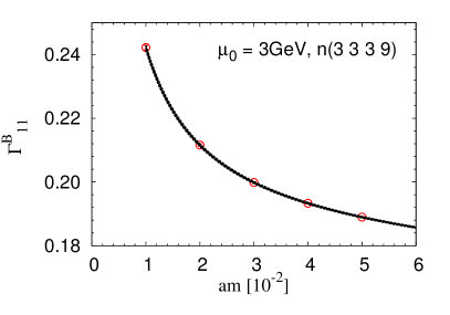
First, we present the data analysis of diagonal terms. Let us consider the element $\Gamma^{B}_{11}$ of $\hat{\Gamma}^{B}$ matrix. We measure the data for 5 valence quark masses and 9 external momenta. The scale of raw data is determined by external momentum ($\mu=|\widetilde{p}|$). Hence, we convert the scale of raw data to the common scale $\mu_{0}=3\mathop{\rm GeV}\nolimits$ using two-loop RG evolution [6]. We fit the data with respect to quark mass for a fixed momentum to the following function $f$ suggested from Ref. [7] based on the Weinberg theorem [8].

$$f(m,a,\widetilde{p})=c_{1}+c_{2}\cdot(am)+c_{3}\cdot\frac{1}{(am)}+c_{4}\cdot\frac{1}{(am)^{2}},$$ (24)

where $m$ is a valence quark mass. After m-fit, we take the $c_{1}(a\widetilde{p})$ as chiral limit values. Because of the sea quark determinant contributions ($c_{3},c_{4}\propto(m^{2}_{\ell}m_{s})^{\nu}$) with $\nu$ the number of zero modes, these pole terms contributions vanish in the chiral limit. The fitting results are presented in Table 1 and Fig. 1(a).

$\mu_{0}$	$c_{1}$	$c_{2}$	$c_{3}$	$c_{4}$	$\chi^{2}/\text{dof}$
3GeV	0.17991(20)	-0.0975(15)	0.0007118(85)	-0.000000790(36)	0.00194(40)

Table 1: m-fit

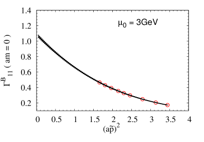
We fit $c_{1}(a\widetilde{p})$ to the following fitting function.

$$g(a\widetilde{p}) =b_{1}+b_{2}\cdot(a\widetilde{p})^{2}+b_{3}\cdot((a\widetilde{p})^{2})^{2}+b_{4}\cdot(a\widetilde{p})^{4}+b_{5}\cdot((a\widetilde{p})^{2})^{3}$$ (25)

To avoid non-perturbative effects at small $(a\widetilde{p})^{2}\leq 1$, we choose the momentum window as $(a\widetilde{p})^{2}>1$. Because we assume that those terms of $\mathcal{O}((a\widetilde{p})^{2})$ and higher order are pure lattice artifacts, we take the $b_{1}$ as $\Gamma^{B}_{11}$ value at $\mu_{0}=3\mathop{\rm GeV}\nolimits$ in the RI-MOM scheme. The fitting result and plot are presented in Table 2 and Fig. 1(b).

$\mu_{0}$	$b_{1}$	$b_{2}$	$b_{3}$	$b_{4}$	$b_{5}$	$\chi^{2}/\text{dof}$
3GeV	1.088(16)	-0.515(18)	0.0953(74)	0.0020(65)	-0.00663(91)	0.08(17)

Table 2: p-fit

(a) m-fit

(b) p-fit

Figure 1: m-fit and p-fit plot at $\mu_{0}=3\mathop{\rm GeV}\nolimits$

Similarly, we analyse the whole elements of $\hat{\Gamma}^{B}$ matrix. Results of diagonal terms in the inverse of $\hat{\Gamma}^{B}$ are

$$X^{-1} =\begin{pmatrix}1.333(32)&-0.793(45)&0.336(21)&0.007(31)\\ -0.726(44)&1.940(41)&-0.008(30)&-0.047(33)\\ 0.341(30)&0.032(45)&1.222(32)&-0.604(37)\\ 0.018(45)&-0.084(52)&-0.637(39)&1.543(36)\end{pmatrix}$$ (26)

$$X^{-1}YY^{T}X^{-1} =\begin{pmatrix}0.0127(15)&-0.0079(11)&0.0020(17)&-0.0001(10)\\ -0.00713(92)&0.0064(11)&-0.0010(11)&-0.00045(73)\\ 0.0020(18)&0.0000(15)&0.0200(90)&-0.0103(48)\\ 0.0001(12)&-0.0012(11)&-0.0109(52)&0.0059(28)\end{pmatrix}$$ (27)

We obtain $\vec{z}$ in RI-MOM scheme at $\mu_{0}=3\mathop{\rm GeV}\nolimits$. We convert the scheme from RI-MOM to $\mathop{\rm\overline{MS}}\nolimits$ using two-loop RG evolution. Results are summarized in Table 3.

	RI-MOM(3GeV)	$\mathop{\rm\overline{MS}}\nolimits$(3GeV)
$z_{1}$	0.9666(78)	0.9812(79)
$z_{2}$	1.095(30)	1.111(31)
$z_{3}$	0.9139(73)	0.9277(74)
$z_{4}$	0.898(28)	0.912(29)

Table 3: The $z$-factors in RI-MOM and $\mathop{\rm\overline{MS}}\nolimits$ scheme. Here, the errors are purely statistical.

Now let us switch the gear to the systematic errors. The first systematic error comes from the diagonal correction terms, $X^{-1}YW^{-1}ZX^{-1}\approx X^{-1}YY^{T}X^{-1}$. We quote $E_{diag}\equiv\vec{z}_{\text{tree}}\cdot X^{-1}YY^{T}X^{-1}$ as this error. The second systematic error comes from the off-diagonal correction terms. Their size ($-X^{-1}Y$) are typically less than $7\%$. However, thanks to the wrong taste suppression ($\ll 1\%$) [9], their effect becomes $\ll 0.07\%$. Hence we neglect them without loss of generality. Another systematic error comes from truncated higher order of the two-loop RG evolution factor (RI-MOM$\to\mathop{\rm\overline{MS}}\nolimits$). We quote $E_{t}\equiv z_{i}\cdot\alpha_{s}^{3}$ as this error.

	$\mathop{\rm\overline{MS}}\nolimits$(3GeV)	$E_{diag}$	$E_{t}$	$E_{tot}$
$z_{1}$	0.9812(79)	0.0077	0.0144	0.0163
$z_{2}$	1.111(31)	0.0027	0.0163	0.0165
$z_{3}$	0.9277(74)	0.0101	0.0136	0.0171
$z_{4}$	0.912(29)	0.0050	0.0134	0.0143

Table 4: The systematic errors of $z$-factors in $\mathop{\rm\overline{MS}}\nolimits$ scheme at $3\mathop{\rm GeV}\nolimits$. $E_{tot}$ represents the total systematic error.

We add these systematic errors ($E_{diag}$ and $E_{t}$) in quadrature as summarized in Table 4.

In addition, we compare the NPR result($\mathop{\rm\overline{MS}}\nolimits$ [NDR]) with those of one-loop perturbative matching. We quote truncated two-loop uncertainty: $E_{t}^{\text{one-loop}}\equiv z_{i}\cdot\alpha_{s}^{2}$ as our estimate of the systematic error of one-loop matching.

	NPR(3GeV)	one-loop(3GeV)	$\Delta$
$z_{1}$	0.981(8)(16)	1.035(62)	0.83 $\sigma$
$z_{2}$	1.111(31)(17)	1.120(67)	0.12 $\sigma$
$z_{3}$	0.928(7)(17)	1.043(63)	1.75 $\sigma$
$z_{4}$	0.912(29)(14)	0.953(57)	0.63 $\sigma$

Table 5: Comparison NPR results and one-loop perturbative matching factors at $3\mathop{\rm GeV}\nolimits$.

Here, note that the results of NPR are consistent with those of one-loop matching within $2\sigma$. This indicates that our NPR results are quite reasonable.

4 Acknowledgments

The research of W. Lee is supported by the Creative Research Initiatives Program (No. 2014001852) of the NRF grant funded by the Korean government (MEST). W. Lee would like to acknowledge the support from KISTI supercomputing center through the strategic support program for the supercomputing application research (KSC-2013-G2-005).

References

• [1] Particle Data Group Collaboration, K. Olive et al. Chin.Phys. C38 (2014) 090001.
• [2] J. Bailey, Y.-C. Jang, and W. Lee PoS LATTICE2014 (2014) 371.
• [3] Y. Aoki, P. Boyle, N. Christ, C. Dawson, M. Donnellan, et al. Phys.Rev. D78 (2008) 054510, [0712.1061].
• [4] J. Kim, J. Kim, W. Lee, and B. Yoon PoS LATTICE2013 (2013) 308, [1310.4269].
• [5] A. T. Lytle and S. R. Sharpe Phys.Rev. D88 (2013), no. 5 054506, [1306.3881].
• [6] J. Kim, W. Lee, J. Leem, S. R. Sharpe, and B. Yoon Phys.Rev. D90 (2014) 014504, [1404.2368].
• [7] T. Blum, N. H. Christ, C. Cristian, C. Dawson, G. T. Fleming, et al. Phys.Rev. D66 (2002) 014504, [hep-lat/0102005].
• [8] S. Weinberg Phys.Rev. 118 (1960) 838–849.
• [9] W. Lee UMI-96-06917-mc (microfiche) 1995. Ph.D. Thesis (Columbia University).