Magnetic Excitations in the Spin-Spiral State of TbMnO₃ and DyMnO₃

Abstract

We calculate spectra of magnetic excitations in the spin-spiral state of perovskite manganates. The spectra consist of several branches corresponding to different polarizations and different ways of diffraction from the static magnetic order. Goldstone modes and opening of gaps at zero and non-zero energies due to the crystal field and the Dzyaloshinski-Moriya anisotropies are discussed. Comparing results of the calculation with available experimental data we determine values of effective exchange parameters and anisotropies. To simplify the spin-wave calculation and to get a more clear physical insight in the structure of excitations we use the $\sigma$-model-like effective field theory to analyze the Heisenberg Hamiltonian and to derive the spectra.

I Introduction

Terbium and Dysprosium manganates, TbMnO₃ and DyMnO₃, are the key materials in the family of multiferroic oxides Kimura2003 ; Goto2004 . Properties of TbMnO₃ and DyMnO₃ are very similar, to be specific below we consider TbMnO₃. Similar to the parent compound of the rare-earth manganites LaMnO₃, TbMnO₃ has orthorhombic lattice structure with lattice constants $a\approx 5.302\AA$, $b=5.857\AA$, and $c=7.402\AA$, Ref. Blasco2000 Below we measure components of wave vectors in units $1/a$, $1/b$, and $1/c$ accordingly. There are three different magnetic phase transitions in TbMnO₃ upon cooling Kajimoto2004 ; Kenzelmann2005 . An incommensurate collinear spin-density wave with the wave vector directed along b, ${\bm{Q}}\approx\pi(0,0.28,0)$, and Mn spins also aligned along b is stabilized below $T_{N}=42$K. This is the spin-stripe phase which is also called the “sinusoidal phase”. Below $T_{S}=28K$ Mn spins reorient into an incommensurate spin spiral. The wave vector of the spiral is practically the same as that in the spin stripe phase, Mn spins are confined in the bc-plane. Finally Tb spins order below $T=7$K. Last but not least, simultaneously with the transition into the spin-spiral phase an electric polarization along c appears at $T=T_{S}$ Kimura2003 . The polarization is coupled with the spin-spiral due to the Dzyaloshinski-Moriya interaction Katsura2005 ; Mostovoy2006 .

In the present work we concentrate on magnetic properties and do not consider ferroelectricity. The major magnetic properties are related to Mn ions. On the other hand Tb ions, which order at the relatively low temperature, play a minor role. In our analysis we disregard Tb ions. There are two very important points concerning magnetic properties of the rare-earth manganites: (i) Magnetic excitations in the spin-spiral phase measured in Ref. Senff2008 are quite unusual. (ii) Even more unusual is the spin-spiral to spin-stripe phase transition at $T=T_{s}$. The phase transition has been considered phenomenologically within an effective Landau-Ginzburg theory in Ref. Mostovoy2006 . We believe that physics behind points (i) and (ii) are closely related, the unusual excitation spectrum is behind the unusual phase transition. In the present paper we address only the first point, we calculate magnetic excitations in the spin-spiral phase. A brute force spin-wave calculation of excitations in the spin-spiral phase is certainly possible, but it is rather technically involved. More importantly such a calculation is not transparent physically. Because of this reason we employ a much more transparent/efficient $\sigma$-model like field theory to find excitations. A similar approach was used previously for calculation of magnetic excitations in the spin-spiral compounds FeSrO₃ and FeCaO₃ Milstein2011 . The field theory is well justified at small momenta, while close to the boundary of magnetic Brillouin zone it can have up to 20-30% inaccuracy. We sacrifice this to get a transparent description of the most important incommensurate physics at small momenta. Structure of the paper is the following: In Section II we consider collinear antiferromagnet LaMnO₃ and formulate the field theory. In this case the spin-wave calculation is straightforward and we compare it with the field theory. In Section III we calculate magnetic excitations in the spin-spiral phase without account of anisotropies and discuss Goldstone modes. Influence of the single ion anisotropy on excitation spectra is considered in Section IV. In Section V we consider the combined influence of the single ion anisotropy and the Dzyaloshinski-Moriya anisotropy on excitation spectra. All the plots in Sections III, IV, and V are presented at values of parameters which reproduce the experimental spectra from Ref. Senff2008 . Those readers who are not interested in details of the calculations can go directly to Section VI where we summarize the results, refer to plots showing the calculated dispersions, and present our conclusions.

II Spin-wave and field theory calculations of magnetic excitations in ${\mbox{LaMnO}}_{3}$

Magnetic structure as well as magnetic excitations in LaMnO₃ have been determined by neutron scattering Moussa1996 ; Hirota1996 . In the ab-plane spins of Mn ions are aligned ferromagnetically, while in the c-direction they are aligned antiferromagnetically, Fig.1.

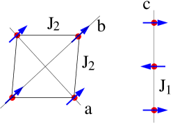
Figure 1: Magnetic structure of LaMnO₃, ferromagnetic ordering in the ab-plane and antiferromagnetic ordering along the c-axis.

The minimal Heisenberg Hamiltonian describing the system is Moussa1996 ; Hirota1996

$$H=J_{1}\sum_{\langle i,j\rangle_{c}}{\vec{S}}_{i}\cdot{\vec{S}}_{j}-J_{2}\sum_{\langle i,j\rangle_{ab}}{\vec{S}}_{i}\cdot{\vec{S}}_{j}\ ,$$ (1)

where $S=2$ is spin of Mn ion, $\langle i,j\rangle_{c}$ denotes nearest neighbours in the c-direction and $\langle i,j\rangle_{ab}$ denotes nearest neighbours in the ab-plane, $J_{1}$ and $J_{2}$ are antiferromagnetic and ferromagnetic exchange integrals indicated in Fig.1. In this work we use the standard definition of exchange integrals: each link in (1) is counted only once. Therefore, our exchange integrals are twice larger than that defined in Refs.Senff2008 ; Moussa1996 ; Hirota1996 . We do not account in (1) the single ion anisotropy because the goal of the present section is just to introduce the field theory. The spin-wave diagonalization of the Hamiltonian (1) is straightforward (a combination of Holstein-Primakoff and Bogoliubov’s transforms). This results in the following magnon dispersion Moussa1996 ; Hirota1996

$$A_{\bm{q}}=J_{1}+2J_{2}(1-\cos q_{a}cosq_{b})$$

$$B_{\bm{q}}=J_{1}\cos q_{c}$$

$$\omega_{\bm{q}}=2S\sqrt{A_{\bm{q}}^{2}-B_{\bm{q}}^{2}}=2S\sqrt{J_{1}^{2}\sin^{2}q_{c}+4J_{1}J_{2}(1-\cos q_{a}cosq_{b})+4J_{2}^{2}(1-\cos q_{a}cosq_{b})^{2}}$$ (2)

It is well known that in the long wave-length limit, $q\ll\pi$, any quantum antiferromagnet is equivalent to a non-linear $\sigma$-model written in terms of the unit vector ${\vec{n}}$ describing the staggered magnetization. The effective Lagrangian of the $\sigma$-model reads

$${\cal L}=\frac{1}{2}\chi_{\perp}{\dot{\vec{n}}}^{2}-E({\vec{n}})\ ,$$ (3)

where $\chi_{\perp}$ is perpendicular magnetic susceptibility and $E({\vec{n}})$ is energy of elastic deformation of spin fabric.

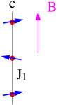
Figure 2: Response of spins to the magnetic field ${\vec{B}}$ applied perpendicular to the staggered magnetization.

The magnetic susceptibility corresponds to the interaction Hamiltonian $H_{B}=-\sum_{i}{\vec{B}}\cdot{\vec{S}}_{i}$, with magnetic field ${\vec{B}}$ applied perpendicular to the staggered magnetization, see Fig.2. A simple calculation shows that the susceptibility per site is

$$\chi_{\perp}=\frac{1}{4J_{1}}\ .$$ (4)

The elastic energy corresponding to the Hamiltonian (1) is

$$E=-S^{2}{\vec{n}}R_{0}(\bm{p}){\vec{n}}+const\ ,$$

$$R_{0}=\frac{J_{1}}{4}\cos(2p_{c})+2J_{2}\cos p_{a}\cos p_{b}$$

$$p_{a}=-i\nabla_{a}\ ,\ \ p_{b}=-i\nabla_{b}\ ,\ \ p_{c}=-i\nabla_{c}\ .$$ (5)

Usually $E$ is expanded up to the second order in momentum, $E\to{\vec{n}}\left\{\frac{\rho_{ab}}{2}(p_{a}^{2}+p_{b}^{2})+\frac{\rho_{c}}{2}p_{c}^{2}\right\}{\vec{n}}\to\frac{\rho_{ab}}{2}[(\nabla_{a}{\vec{n}})^{2}+(\nabla_{b}{\vec{n}})^{2}]+\frac{\rho_{c}}{2}(\nabla_{c}{\vec{n}})^{2}$, where $\rho_{ab}$ and $\rho_{c}$ are the corresponding spin stiffnesses. In the present work we do not expand $E$ in powers of momentum, instead we use (II) as it is. Note that the ferromagnetic $J_{2}$-term in (II) is unambiguous, on the other hand the antiferromagnetic $J_{1}$-term is somewhat ambiguous. One can write the antiferromagnetic $J_{1}$-term as it is done in (II) or alternatively as $J_{1}\cos(p_{c})$. In the long-wave length limit the both ways result in the same spin stiffness $\frac{J_{1}}{4}\cos(2p_{c})\to const-J_{1}p_{c}^{2}/2$, and $J_{1}\cos(p_{c})\to const-J_{1}p_{c}^{2}/2$. We use the way (II) because it leads to the correct magnon dispersion up to $p_{c}=\pi/2$, see Eq.(7), and hence allows one to overstretch the region of validity of the field theory com1 .

Minimum of energy (II) defines the ground state which corresponds to the constant staggered magnetization ${\vec{n}}={\vec{n}}_{0}$. Magnetic excitations above the ground state, ${\vec{n}}={\vec{n}}_{0}+\delta{\vec{n}}$, $\delta{\vec{n}}\perp{\vec{n}}_{0}$, are defined by the Euler-Lagrange equation of Lagrangian (3).

$$\chi_{\perp}{\ddot{\delta{\vec{n}}}}=2S^{2}\left[R_{0}({\bm{p}})-R_{0}(0)\right]\delta{\vec{n}}\ .$$ (6)

For $\delta{\vec{n}}=\delta{\vec{n}}_{0}e^{-i\omega_{\bm{q}}t+i{\bm{q}}\cdot{\bm{r}}}$ this results in the dispersion

$$\omega_{\bm{q}}=2S\sqrt{J_{1}^{2}\sin^{2}q_{c}+4J_{1}J_{2}(1-\cos q_{a}cosq_{b})}\ .$$ (7)

Compared to the “exact” spin-wave calculation (II) the term $4J_{2}^{2}(1-\cos q_{a}cosq_{b})^{2}$ is missing under the square root. In the long wave-length limit, $q_{a},q_{b}\ll\pi$, this term is quartic in momenta and therefore it is irrelevant. Moreover, at $J_{2}\ll J_{1}$ this term is irrelevant even at $q_{a},q_{b}=\pi$. The inequality $J_{2}\ll J_{1}$ is certainly not valid for LaMnO₃ where $J_{1}\approx 1.17$ meV and $J_{2}\approx 1.66$ meV, see Refs. Moussa1996 ; Hirota1996 . However, we will see that for TbMnO₃ $J_{2}\lesssim J_{1}/2$.

For the collinear magnetic ground state in LaMnO₃ the spin-wave calculation (II) is very simple and therefore application of the field theory does not make sense. The purpose of the present section is just to demonstrate how the field theory works in the known simple case. Below we employ the field theory for the spin-spiral states of TbMnO₃ and DyMnO₃. For a noncollinear state the field theory is significantly more efficient technically.

It is instructive to compare also quantum/thermal fluctuations obtained within the spin-wave theory and within the field theory. The fluctuation reduction of the staggered magnetization within the spin-wave theory is determined by Bogoliubov’s parameters $u_{\bm{q}}$ and $v_{\bm{q}}$:

$$u_{\bm{q}}^{2}=\frac{1}{2}\left(A_{\bm{q}}/\sqrt{A_{\bm{q}}^{2}-B_{\bm{q}}^{2}}+1\right)$$

$$v_{\bm{q}}^{2}=\frac{1}{2}\left(A_{\bm{q}}/\sqrt{A_{\bm{q}}^{2}-B_{\bm{q}}^{2}}-1\right)$$

$$\langle n_{b}\rangle=\frac{\langle S_{b}\rangle}{S}=1-\frac{2}{S}\sum_{q\in MBZ}\left\{v_{\bm{q}}^{2}+(u_{\bm{q}}^{2}+v_{\bm{q}}^{2})f_{\bm{q}}\right\}$$

$$=1-\sum_{q\in MBZ}\left\{\left(\frac{2A_{\bm{q}}}{\omega_{\bm{q}}}-\frac{2}{S}\right)+\frac{4A_{\bm{q}}}{\omega_{\bm{q}}}f_{\bm{q}}\right\}\ .$$ (8)

Here $f_{\bm{q}}=\left(e^{\omega_{\bm{q}}/T}-1\right)^{-1}$ is the Bose thermal occupation factor. The summation over momentum is performed inside the Magnetic Brillouin Zone (MBZ), $-\pi/2\leq q_{c}\leq\pi/2$, $-\pi\leq q_{a},q_{b}\leq\pi$. The fluctuation reduction within the field theory is of the following form Milstein2011

$$\langle n_{b}\rangle=1-\sum_{q\in MBZ}\frac{1}{\chi_{\perp}\omega_{\bm{q}}}\left(\frac{1}{2}+f_{\bm{q}}\right)\ .$$ (9)

At small $q$ the integrand in (9) is equal to that in (II), this is true for both thermal fluctuations (proportional to $f_{\bf q}$) and for quantum fluctuations. Moreover, at $J_{2}\ll J_{1}$ the thermal fluctuation contributions in Eqs. (9) and (II) are equal over the entire MBZ. The large $q$ quantum fluctuation contributions in Eqs. (9) and (II) are generally different. However, for S=2 quantum fluctuations are anyway small and there is no need to consider them.

III Magnetic excitations in the spin-spiral phase of $\mbox{TbMnO}_{3}$ without account of anisotropies

According to Ref. Senff2008 the incommensurate spin structure in TbMnO₃ is due to ab-plane frustrating antiferromagnetic interaction $J_{3b}$

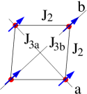
Figure 3: Frustrating ab-plane antiferromagnetic interactions $J_{3b}$ and $J_{3a}$ in TbMnO₃.

shown in Fig.3, for completeness we also introduce $J_{3a}$. So, in TbMnO₃ there is the following addition to the Hamiltonian (1)

$$\delta H=J_{3b}\sum_{\langle i,j\rangle_{b}}{\vec{S}}_{i}\cdot{\vec{S}}_{j}+J_{3a}\sum_{\langle i,j\rangle_{a}}{\vec{S}}_{i}\cdot{\vec{S}}_{j}\ .$$ (10)

Here $\langle i,j\rangle_{b}$ denotes next nearest neighbours along the b-direction and $\langle i,j\rangle_{a}$ denotes the next nearest neighbours along the a-direction. The spin-elastic energy corresponding to $H+\delta H$ is similar to (II)

$$E = -S^{2}{\vec{n}}R(\bm{p}){\vec{n}}+const\ ,$$

$$R = \frac{J_{1}}{4}\cos(2p_{c})+2J_{2}\cos p_{a}\cos p_{b}$$ (11)

$$- J_{3b}\cos(2p_{b})-J_{3a}\cos(2p_{a})\ .$$

Below we assume that

$$J_{2}<2J_{3b},\ \ \ \ J_{2}^{2}>4J_{3a}J_{3b}\ .$$ (12)

In this case it is easy to check that the energy (III) is minimum for the spin spiral ground state

$${\vec{n}}_{0}={\vec{e}}_{1}\cos(\bm{Q}\cdot\bm{r})+{\vec{e}}_{2}\sin(\bm{Q}\cdot\bm{r})\,,$$

$$\bm{Q}=Q\bm{e}_{b}\,,\quad\cos Q=\frac{J_{2}}{2J_{3b}}\,,$$ (13)

where ${\vec{e}}_{1}$ and ${\vec{e}}_{2}$ are two arbitrary orthogonal unit vectors which define plane of the spiral. According to Ref. Senff2008 in TbMnO₃ the wave vector is $Q\approx 0.28\pi$, hence $J_{2}/J_{3b}\approx 1.27$.

In-plane excitations.
There are two types of magnetic excitations in the spin spiral state, in-plane spin excitation and out-of-plane spin excitation. The in-plane excitation is described by a phase $\varphi(t,{\bm{r}})$, $\varphi\ll 1$, it results in the following vector ${\vec{n}}$,

$${\vec{n}}={\vec{e}}_{1}\cos(\bm{Q}\cdot\bm{r}+\varphi)+{\vec{e}}_{2}\sin(\bm{Q}\cdot\bm{r}+\varphi)\,,$$

$$\approx\left(1-\varphi^{2}/2\right){\vec{n}}_{0}+\varphi{\vec{n}}_{1}\,,$$

$${\vec{n}}_{1}=-{\vec{e}}_{1}\sin(\bm{Q}\cdot\bm{r})+{\vec{e}}_{2}\cos(\bm{Q}\cdot\bm{r})\,.$$ (14)

Substituting this ${\vec{n}}$ in Eqs.(3),(III) and taking variation with respect to $\varphi$ we find the following Euler-Lagrange equation

$$-\chi_{\perp}{\ddot{\varphi}}+2S^{2}[-\varphi{\vec{n}}_{0}R(\bm{p}){\vec{n}}_{0}+{\vec{n}}_{1}R(\bm{p}){\vec{n}}_{1}\varphi]=0\,.$$ (15)

Having in mind the plane wave solution, $\varphi=\varphi_{0}\exp(-i\omega_{\bm{q}}t+i\bm{q}\cdot\bm{r})$, we note that the following relations are valid

$${\vec{n}}_{1}R(\bm{p}){\vec{n}}_{1}e^{i\bm{q}\cdot\bm{r}}=\frac{1}{2}[R(\bm{q}+\bm{Q})+R(\bm{q}-\bm{Q})]e^{i\bm{q}\cdot\bm{r}}$$

$${\vec{n}}_{0}R(\bm{p}){\vec{n}}_{0}=R(\bm{Q})\ .$$ (16)

Hence Eq.(15) results in the following spectrum of the in-plane excitation

$$\omega_{\bm{q}}^{(in)}=2S\sqrt{J_{1}[2R(\bm{Q})-R(\bm{q}+\bm{Q})-R(\bm{q}-\bm{Q})]}\,.$$ (17)

As one should expect $\omega_{\bm{q}}^{(in)}=0$ for $\bm{q}=0$. This is the Goldstone sliding mode.

Out-of-plane excitations.
The out-of-plane excitation $h(t,{\bm{r}})$, $h\ll 1$, results in the following vector ${\vec{n}}$,

$${\vec{n}}=\sqrt{1-h^{2}}\,{\vec{n}}_{0}+h{\vec{e}}_{3}\approx\left(1-h^{2}/2\right){\vec{n}}_{0}+h{\vec{e}}_{3}\,,$$ (18)

where ${\vec{e}}_{3}=[{\vec{e}}_{1}\times{\vec{e}}_{2}]$ is a unit vector perpendicular to the plane of spiral. Substituting (18) in Eqs.(3),(III) and performing variation with respect to $h$, we get the following Euler-Lagrange equation

$$-\chi_{\perp}{\ddot{h}}+2S^{2}[-h{\vec{n}}_{0}R(\bm{p}){\vec{n}}_{0}+{\vec{e}}_{3}R(\bm{p}){\vec{e}}_{3}h]=0\,.$$ (19)

The plane-wave solution, $h=h_{0}\exp(-i\omega_{\bm{q}}t+i\bm{q}\cdot\bm{r})$, gives the following spectrum of the out-of-plane excitation

$$\omega_{\bm{q}}^{(out)}=2S\sqrt{2J_{1}[R(\bm{Q})-R(\bm{q})]}\,.$$ (20)

The dispersion has two zeroes (Goldstone modes) $\omega_{\bm{q}}^{(out)}=0$ for $\bm{q}=\pm{\bm{Q}}$.

Altogether the spectrum has three Goldstone modes corresponding to three possible rotations of the spin spiral. The in-plane sliding mode with $q=0$ corresponds to the rotation around ${\vec{e}}_{3}$, and two out-of-plane modes with $\bm{q}=\pm{\bm{Q}}$ correspond to linear combinations of rotations around ${\vec{e}}_{1}$ and ${\vec{e}}_{2}$.

Comparison with experiment.
Dispersions of two branches (17) and (20) have been derived without account of anisotropies. The anisotropies, which we consider later, significantly modify the dispersions at small momenta. However, close to boundaries of MBZ, where excitation energies are sufficiently high, influence of anisotropies is relatively small. Therefore, to estimate values of the exchange integrals we calculate $\omega_{\bm{q}}^{(out)}$ at some points at the boundary of MBZ. According to Eq.(20)

$${\bm{q}}=(0,Q,\frac{\pi}{2}),\ \ \ \omega_{\bm{q}}^{(out)}=2SJ_{1}$$

$${\bm{q}}=(\pi,Q,0),\ \ \ \ \omega_{\bm{q}}^{(out)}=5.1S\sqrt{J_{1}J_{3b}}$$

$${\bm{q}}=(0,\pi,0),\ \ \ \ \ \omega_{\bm{q}}^{(out)}=6.5S\sqrt{J_{1}J_{3b}}$$ (21)

Comparing this with data presented in Figs.8,10 from Ref. Senff2008 we find approximate values of the exchange integrals

$$J_{1}\approx 0.9\,\mbox{meV}\,,\,J_{2}\approx 0.38\,\mbox{meV}$$

$$J_{3b}\approx 0.3\,\mbox{meV}\,,\,J_{3a}=0.1\,\mbox{meV}\,.$$ (22)

Note that $J_{2}$ follows from Eq.(III) as soon as $J_{3b}$ is determined. There are no data to determine $J_{3a}$. Rather arbitrarily we take $J_{3a}=0.1$meV which satisfies the inequality (12). Values of $J_{2}$, $J_{3b}$, and $J_{3a}$ presented in (22) are probably slightly larger than the real ones ($\sim$20%) because of the inaccuracy of the field theory close to the boundary of MBZ. Values of exchange integrals in Eq. (22) reasonably agree with that derived in Ref. Senff2008 (We remind that our integrals are formally by factor 2 larger due to the different definition).

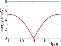
Figure 4: The in-plane magnon dispersion without account of anisotropies. The dispersion is shown along the ${\bm{q}}=(0,q_{b},0)$ direction.

The in-plane dispersion (17) has minimum at $q=0$. The dispersion for ${\bm{q}}=(0,q_{b},0)$ is shown in Fig.4. The in-plane excitation shown in Fig.4 cannot be seen directly in neutron scattering since the corresponding n-field (III) contains an additional oscillating factor $\cos(\bm{Q}\cdot\bm{r})$ or $\sin(\bm{Q}\cdot\bm{r})$. Therefore in a scattering measurement the in-plane mode is seen as two shifted branches $\omega^{in}({\bm{q}}\pm{\bm{Q}})$ with half intensity each. These branches are shown by red dashed lines in Fig.5, panels A and B, along three different directions. Note, there is a crossing in panel B at $q_{a}=\pm 2Q$. The out-of-plane excitation (18),(20) can be seen in inelastic neutron scattering as it is. The corresponding dispersion (20) along three different directions is plotted in Fig.5, panels C and D, by black solid lines.

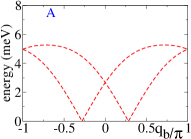
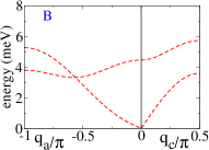
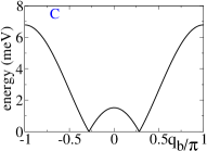
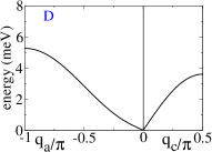
Figure 5: Magnon dispersions (as they are seen in neutron scattering) without account of anisotropies. Panels A and B: branches of the in-plane dispersion $\omega^{in}({\bm{q}}\pm{\bm{Q}})$. Panels C and D: out-of-plane dispersion $\omega^{out}({\bm{q}})$. Panels A and C correspond to q along b, ${\bm{q}}=(0,q_{b},0)$. Panels B and D correspond to ${\bm{q}}={\bm{Q}}+\delta{\bm{q}}$, where $\delta{\bm{q}}$ is directed along a and c.

IV Excitation spectra with account for the crystal field anisotropy along the b-axis

Different anisotropies influence the magnon spectra in different ways. In this section we consider only the crystal field anisotropy along the b-axis. The corresponding correction to the elastic energy (III) is

$$H_{cf}=-\Lambda S_{b}^{2}=-\Lambda S^{2}n_{b}^{2}\ ,$$ (23)

where $\Lambda>0$ is the strength of the crystal field. While in the present work we consider only the spin-spiral phase, the sign of $\Lambda$ (“easy axis” anisotropy) is dictated by the spin-stripe phase, where spin is directed along b. We assume that $\Lambda$ is sufficiently small and therefore consider only effects linear in $\Lambda$. Dispersion plots presented below correspond to

$$\Lambda=0.125\ {\mbox{meV}}\ ,$$ (24)

which is approximately consistent with the neutron scattering data Senff2008 . The crystal field (23) results in two static effects. (i) The plane of the spin spiral must include the axis b. So, while in Eq.(III) vectors ${\bm{e}}_{1}$ and ${\bm{e}}_{2}$ are arbitrary orthogonal unit vectors, now we take

$${\bm{e}}_{2}={\bm{e}}_{b}\ ,\ \ \ {\bm{e}}_{1}\perp{\bm{e}}_{b}\ ;$$ (25)

(ii) The spin spiral gets an additional static position dependent phase $\varphi_{st}({\bm{r}})$. So (III) is replaced by

$${\vec{N}}_{0} = {\vec{e}}_{1}\cos(\bm{Q}\cdot\bm{r}+\varphi_{st})+{\vec{e}}_{2}\sin(\bm{Q}\cdot\bm{r}+\varphi_{st})$$ (26)

$$= \cos\varphi_{st}\,{\vec{n}}_{0}+\sin\varphi_{st}\,{\vec{n}}_{1}\,.$$

Static deformation of the spin spiral.
Minimization of energy $E+H_{cf}$, Eqs. (III),(23), results in the following equation for $\varphi_{st}$

$$[-\varphi_{st}{\vec{n}}_{0}R(\bm{p}){\vec{n}}_{0}+{\vec{n}}_{1}R(\bm{p}){\vec{n}}_{1}\varphi_{st}]=-\Lambda\sin(2\bm{Q}\cdot\bm{r})\,.$$ (27)

Solution of this equation is

$$\varphi_{st}({\bm{r}})=-\frac{\Lambda\sin(2\bm{Q}\cdot\bm{r})}{R(3\bm{Q})-R(\bm{Q})}=\frac{\Lambda\sin(2\bm{Q}\cdot\bm{r})}{8J_{3b}\sin^{2}(2Q)\sin^{2}Q}\,.$$ (28)

The phase of the spin spiral (26) is $\Phi=\bm{Q}\cdot\bm{r}+\varphi_{st}$. The phase has a zero mode corresponding to the shift ${\bm{r}}\to{\bm{r}}+\delta{\bm{r}}$

$$\varphi({\bm{r}})\propto\frac{\partial\Phi({\bm{r}})}{\partial({\bm{Q}}\cdot{\bm{r}})}=\left\{1-\frac{2\Lambda\cos(2\bm{Q}\cdot\bm{r})}{R(3\bm{Q})-R(\bm{Q})}\right\}\,.$$ (29)

This is the Goldstone sliding mode which remains gapless in presence of anisotropy, $\omega_{q=0}^{(in)}=0$.

In-plane excitations.
According to the discussion in the previous paragraph, the in-plane excitation remains gapless even with the anisotropy. The only qualitatively visible effect of the anisotropy is discontinuity of the dispersion due to diffraction of magnons from the static spin spiral. The dispersion is discontinuous at $q_{b}=Q$ and $q_{b}=\pi-Q$.

To find the in-plane excitation with nonzero energy $\varphi(t,{\bm{r}})$ we represent the vector ${\vec{n}}$ similar to (III)

$${\vec{n}}={\vec{e}}_{1}\cos(\bm{Q}\cdot\bm{r}+\varphi_{st}+\varphi)+{\vec{e}}_{2}\sin(\bm{Q}\cdot\bm{r}+\varphi_{st}+\varphi)\,,$$

$$\approx\left(1-\frac{\varphi^{2}}{2}\right){\vec{N}}_{0}+\varphi{\vec{N}}_{1}\,,$$

$${\vec{N}}_{1}=-{\vec{e}}_{1}\sin(\bm{Q}\cdot\bm{r}+\varphi_{st})+{\vec{e}}_{2}\cos(\bm{Q}\cdot\bm{r}+\varphi_{st})\,,$$ (30)

The corresponding Euler-Lagrange equation is

$$-\chi_{\perp}{\ddot{\varphi}}+2S^{2}[-\varphi{\vec{N}}_{0}R(\bm{p}){\vec{N}}_{0}+{\vec{N}}_{1}R(\bm{p}){\vec{N}}_{1}\varphi]$$

$$+2\Lambda S^{2}\varphi\cos(2\bm{Q}\cdot\bm{r})=0\,.$$ (31)

It is easy to check that the zero frequency sliding mode solution (29) satisfies this equation.

The spin spiral in combination with the crystal field anisotropy (23) generates the effective scattering “potential” with momentum $\Delta{\bm{q}}=2{\bm{Q}}$. As usual, the scattering is most pronounced when the “resonance” condition, $\omega_{\bm{q}}^{(in)}=\omega_{\bm{q}\pm 2{\bm{Q}}}^{(in)}$, is fulfilled. The condition is fulfilled at ${\bm{q}}={\bm{q}}_{\perp}+{\bm{Q}}=(q_{a},Q,q_{c})$ and at ${\bm{q}}={\bm{q}}_{\perp}+{\bm{\pi}}_{b}-{\bm{Q}}=(q_{a},\pi-Q,q_{c})$. At these planes the magnon spectrum becomes discontinuous. Eq.(IV), which describes magnon diffraction, is similar to the Schrodinger equation for electron band structure. The only difference is that the Schrodinger equation contains the electron energy, while Eq.(IV) contains $\omega^{2}$. Solution of Eq.(IV) is obvious from this analogy,

$$(\Omega_{\bm{q}}^{(in)})^{2} = \frac{1}{2}[(\omega_{\bm{q}}^{(in)})^{2}+(\omega_{\bm{q}\pm 2\bm{Q}}^{(in)})^{2}]$$ (32)

$$\pm \sqrt{\frac{1}{4}[(\omega_{\bm{q}}^{(in)})^{2}-(\omega_{\bm{q}\pm 2\bm{Q}}^{(in)})^{2}]^{2}+M_{\bm{q}}^{2}}\,.$$

The sign $\pm$ before the square root and the sign $\pm$ in $\bm{q}\pm 2\bm{Q}$ depend on the momentum $q_{b}$. The choice of the signs must correspond to the standard band theory convention. The mixing matrix element $M_{\bm{q}}$ is different for $q_{b}\approx Q$ and for $q_{b}\approx\pi-Q$. How to find values of the matrix element? Let us, for example, take ${\bm{q}}=(q_{a},Q,q_{c})$. Here the solution of Eq.(IV) must be of the following form, $\varphi\propto e^{iq_{a}a+iq_{c}c}\psi_{b}$, where $\psi_{b}=\cos(Qb)$ or $\psi_{b}=\sin(Qb)$. Substitution of these two solutions in Eq.(IV) allows one to find corresponding frequency $(\Omega_{\bm{q}}^{(in)})^{2}$. On the other hand, according to (32) the frequencies are $(\Omega_{\bm{q}}^{(in)})^{2}=(\omega_{\bm{q}}^{(in)})^{2}\pm M_{\bm{q}}$. Comparing we find value of the matrix element. This calculation gives the following results

$$q_{b}\approx Q:$$ (33)

$$M_{\bm{q}}=4\Lambda J_{1}S^{2}\left\{\frac{3}{2}+\frac{R(q_{a},0,q_{c})-R(q_{a},2Q,q_{c})}{R(3\bm{Q})-R(\bm{Q})}\right\}$$

$$q_{b}\approx\pi-Q:$$

$$M_{\bm{q}}=4\Lambda J_{1}S^{2}\left\{\frac{3}{2}+\frac{R(q_{a},\pi,q_{c})-R(q_{a},\pi-2Q,q_{c})}{R(3\bm{Q})-R(\bm{Q})}\right\}$$

The in-plane dispersion $\Omega^{(in)}_{\bm{q}}$ for ${\bm{q}}=(0,q_{b},0)$ is shown in Fig.6.

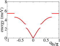
Figure 6: In-plane magnon dispersion with account of the crystal field anisotropy (23). The dispersion is shown along the ${\bm{q}}=(0,q_{b},0)$ direction.

Discontinuities of the dispersion due to diffraction of magnons from the static spin spiral are clearly seen. We already pointed out that the in-plane excitation cannot be seen directly in neutron scattering since the corresponding n-field (III) contains an additional oscillating factor $\cos(\bm{Q}\cdot\bm{r})$ or $\sin(\bm{Q}\cdot\bm{r})$. Therefore in a scattering measurement the in-plane mode is seen as two shifted branches $\Omega^{in}({\bm{q}}\pm{\bm{Q}})$ with half intensity each. These branches for three different momentum directions are shown by red dashed lines in Fig.7, panels A and B.

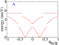
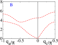
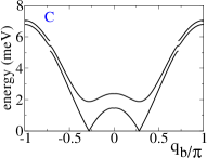
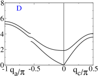
Figure 7: Magnon dispersions (as they seen in neutron scattering) with account of the crystal field anisotropy (23). Panels A and B: branches of the in-plane dispersion $\Omega^{in}({\bm{q}}\pm{\bm{Q}})$. Panels C and D: branches of the out-of-plane dispersion $\Omega^{out1}({\bm{q}})$, $\Omega^{out2}({\bm{q}})$. Panels A and C correspond to q along b, ${\bm{q}}=(0,q_{b},0)$. Panels B and D correspond to ${\bm{q}}={\bm{Q}}+\delta{\bm{q}}$, where $\delta{\bm{q}}$ is directed along a and c.

Out-of-plane excitations.
There are two anisotropy induced effects on the out-of-plane excitations, (i) opening of the gap at zero frequency, (ii) discontinuity of the dispersion due to diffraction of magnons from the static spin spiral. Without an anisotropy there are two out-of-plane Goldstone modes with $\bm{q}=\pm{\bm{Q}}$ corresponding to linear combinations of rotations around ${\vec{e}}_{1}$ and ${\vec{e}}_{2}$, see Fig.5C, black solid line. The anisotropy (23) does not respect rotations around ${\vec{e}}_{1}$, but it does respect rotations around ${\vec{e}}_{2}={\vec{e}}_{b}$. Therefore, we expect one gapless and one gapped out-of-plane mode.

For out-of plane fluctuations we have

$${\vec{n}}=\sqrt{1-h^{2}}{\vec{N}}_{0}+h{\vec{e}}_{3}\,,$$ (34)

and the corresponding Euler-Lagrange equation is

$$-\chi_{\perp}{\ddot{h}}+2S^{2}[-h{\vec{N}}_{0}R(\bm{p}){\vec{N}}_{0}+{\vec{e}}_{3}R(\bm{p}){\vec{e}}_{3}h]$$

$$-S^{2}\Lambda[1-\cos(2\bm{Q}\cdot\bm{r}+2\varphi_{st})]h=0\,.$$ (35)

Expanding this equation up to the first order in $\Lambda$ we get

$$-\chi_{\perp}{\ddot{h}}+2S^{2}[R(\bm{p})-R(\bm{Q})]h$$

$$=S^{2}\Lambda[1-2\cos(2\bm{Q}\cdot\bm{r})]h\,.$$ (36)

It is easy to check that at $\bm{q}=\bm{Q}$ this equation has a gapless solution

$$\Omega_{\bm{Q}}^{(out1)}=0,\ \ \ h\propto\cos(\bm{Q}\cdot\bm{r}).$$ (37)

and a gapped solution

$$\Omega_{\bm{Q}}^{(out2)}=\sqrt{8S^{2}J_{1}\Lambda},\ \ \ h\propto\sin(\bm{Q}\cdot\bm{r}).$$ (38)

In $\cos(\bm{Q}\cdot\bm{r})$ and $\sin(\bm{Q}\cdot\bm{r})$ solutions we neglect higher harmonics terms which have small amplitudes $\sim\Lambda/J_{1}$. Thus, the spectrum near its minimum agrees with our expectations.

Eq.(IV) contains the effective scattering “potential” with momentum $\Delta{\bm{q}}=2{\bm{Q}}$. Hence there must be a discontinuity of the spectrum at $q_{b}=\pm(\pi-Q)$. Similarly to (32), the spectrum in the vicinity of this momentum is

$$(\Omega_{\bm{q}}^{(out)})^{2}\approx\frac{1}{2}[(\omega_{\bm{q}}^{(out)})^{2}+(\omega_{\bm{q}+2\bm{Q}}^{(out)})^{2}]$$

$$\pm\sqrt{\frac{1}{4}[(\omega_{\bm{q}}^{(out)})^{2}-(\omega_{\bm{q}+2\bm{Q}}^{(out)})^{2}]^{2}+(4J_{1}S^{2}\Lambda)^{2}}\,.$$ (39)

The out-of-plane excitations are seen in inelastic neutron scattering as they are. Dispersions $\Omega_{\bm{q}}^{(out1)}$ and $\Omega_{\bm{q}}^{(out2)}$ along three different directions are plotted in Fig.7, panels C and D, by black solid lines.

V Excitation spectra with account of both the crystal field anisotropy and the Dzyaloshinski-Moriya anisotropy

The effective Dzyaloshinski-Moriya (DM) interaction between the ferroelectric polarization ${\vec{P}}$ and spins is of the following form Katsura2005 ; Mostovoy2006

$$H_{DM}\propto{\vec{P}}\cdot\left[{\vec{e}}_{12}\times\left[{\vec{S}}_{1}\times{\vec{S}}_{2}\right]\right]\ ,$$ (40)

where ${\vec{S}}_{1}$ and ${\vec{S}}_{2}$ are spins at nearest sites and ${\vec{e}}_{12}$ is a unit vector directed from the site 1 to the site 2. Here we consider the case of zero external magnetic field when the polarization ${\vec{P}}$ is directed along the c-axis Kimura2003 . The vector ${\vec{e}}_{12}$ is directed along the b-axis and hence the interaction (40) put the spin spiral in the bc-plane.

$${\bm{e}}_{2}={\bm{e}}_{b}\ ,\ \ \ {\bm{e}}_{1}={\bm{e}}_{c}\ .$$ (41)

Eq. (40) can be rewritten in terms of the unit vector ${\vec{n}}$ describing the magnetization staggered in the c-direction,

$$H_{DM}={\cal D}S^{2}[\vec{n}\times\nabla_{b}\vec{n}]_{a}\to const+{\cal D}QS^{2}n_{a}^{2}\ ,$$ (42)

where ${\cal D}>0$ is the constant of the DM interaction. So, in these notations the DM interaction is equivalent to the crystal field anisotropy with the coefficient in the effective crystal field proportional to the wave vector of the spin spiral. The coefficient ${\cal D}$ is related to the ferroelectric polarization and therefore it is strongly temperature dependent. In particular ${\cal D}=0$ in the spin stripe phase at $T>T_{S}$. However, here we consider the system deep in the spin spiral phase, $T<T_{S}$, and for numerical estimates we use

$${\cal D}=0.20\ {\mbox{meV}}\ ,$$ (43)

which results in spectra approximately consistent with the neutron scattering data Senff2008 .

In-plane excitations.
The DM anisotropy obviously does not influence the in-plane spin fluctuations. Therefore the in-plane excitation spectra derived in Section IV are fully valid in this case. In Fig.8 we present magnetic excitation spectra with account of both the crystal field anisotropy and the Dzyaloshinski-Moriya anisotropy. Panels A and B in Fig.8 are identical to that in Fig.7.

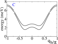
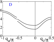
Figure 8: Magnon dispersions (as they seen in neutron scattering) with account of both the crystal field anisotropy (23) and the Dzyaloshinski-Moriya anisotropy (40),(42). Panels A and B: branches of the in-plane dispersion $\Omega^{in}({\bm{q}}\pm{\bm{Q}})$. Panels C and D: branches of the out-of-plane dispersion $\Omega^{out1}({\bm{q}})$, $\Omega^{out2}({\bm{q}})$. Panels A and C correspond to q along b, ${\bm{q}}=(0,q_{b},0)$. Panels B and D correspond to ${\bm{q}}={\bm{Q}}+\delta{\bm{q}}$, where $\delta{\bm{q}}$ is directed along a and c.

Out-of-plane excitations.
We remind that even with the crystal field anisotropy but without of the DM anisotropy one of the out-of-plane excitations modes remains gapless, see panels C and D in Fig.7. The most notable effect of the DM anisotropy is opening of a gap in the remaining gapless mode. With account of the anisotropy Eqs. (IV), (37), and 38) are modified as

$$-\chi_{\perp}{\ddot{h}}+2S^{2}[R(\bm{p})-R(\bm{Q})]h$$

$$=S^{2}\left\{\Lambda[1-2\cos(2\bm{Q}\cdot\bm{r})]+{\cal D}Q\right\}h\,.$$ (44)

At $\bm{q}=\bm{Q}$ this equation has two gapped solutions

$$\Omega_{\bm{Q}}^{(out1)}\approx\sqrt{4S^{2}J_{1}{\cal D}Q},\ \ h\propto\cos(\bm{Q}\cdot\bm{r})$$ (45)

$$\Omega_{\bm{Q}}^{(out2)}\approx\sqrt{4S^{2}J_{1}(2\Lambda+{\cal D}Q)},\ \ h\propto\sin(\bm{Q}\cdot\bm{r})\ .$$

In $\cos(\bm{Q}\cdot\bm{r})$ and $\sin(\bm{Q}\cdot\bm{r})$ solutions we neglect higher harmonics terms which have small amplitudes $\sim\Lambda/J_{1}$.

Similarly to Eq.(IV), Eq.(V) contains the effective scattering “potential” with momentum $\Delta{\bm{q}}=2{\bm{Q}}$. Hence there must be a discontinuity of the spectrum at $q_{b}=\pm(\pi-Q)$. Similarly to (IV), the spectrum in the vicinity of this momentum is

$$(\Omega_{\bm{q}}^{(out)})^{2}\approx\frac{1}{2}[(\omega_{\bm{q}}^{(out)})^{2}+(\omega_{\bm{q}+2\bm{Q}}^{(out)})^{2}]$$ (46)

$$\pm\sqrt{\frac{1}{4}[(\omega_{\bm{q}}^{(out)})^{2}-(\omega_{\bm{q}+2\bm{Q}}^{(out)})^{2}]^{2}+(4J_{1}S^{2}\Lambda)^{2}}\,.$$ (47)

The out-of-plane excitations are seen in inelastic neutron scattering as they are. Dispersions $\Omega_{\bm{q}}^{(out1)}$ and $\Omega_{\bm{q}}^{(out2)}$ along three different directions are plotted in Fig.8, panels C and D, by black solid lines.

VI Conclusions

We have calculated spectra of magnetic excitations in the spin spiral state of perovskite manganates TbMnO₃ and DyMnO₃. As starting point we use the frustrated Heisenberg Hamiltonian $H+\delta H$ suggested in Refs. Moussa1996 ; Hirota1996 ; Senff2008 and determined by Eqs. (1), (10). We also account for the crystal field anisotropy (23) and the Dzyaloshinski-Moriya anisotropy, (40),(42). In the present work we do not consider a relaxation, hence a line broadening is not included in the analysis.

To simplify calculations and to get a physical insight in the structure of magnetic excitations we employ a $\sigma$-model like field theory. At small momenta in the region of the most important and complex incommensurate physic, the field theory is fully equivalent to the Heisenberg model. On the hand, close to the boundary of magnetic Brillouin zone the field theory underestimates the magnon frequency by about 20% compared to the Heisenberg model. Values of parameters which reproduce the measured dispersion in TbMnO₃, Ref. Senff2008 , are listed in Eqs. (22), (24), and (43). Exchange integrals in Eq. (22) are consistent with that in Ref. Senff2008 with account of different definitions (factor 2).

There are in-plane (spin oscillates in the plane of the spin spiral) and out-of-plane excitations (spin oscillates perpendicular to the plane of the spin spiral). Dispersions of the in-plane and the out-of-plane excitations (as they are seen in neutron scattering) without account of the crystal field and Dzyaloshinski-Moriya anisotropies are presented in Fig. 5. All the dispersions are Goldstone ones, the energy is zero at the wave vector equal to the wave vector of the spin spiral.

Account of the crystal field anisotropy leads to the two effects (i) opening of the gap in one of the Goldstone modes, (ii) discontinuity of the dispersion due to diffraction of magnons from the static spin spiral. Dispersions of the in-plane and the out-of-plane excitations (as they are seen in neutron scattering) with account of the crystal field anisotropy but without account of the Dzyaloshinski-Moriya interaction are presented in Fig. 7.

Further account of the Dzyaloshinski-Moriya interaction opens gap in both out-of-plane modes. As expected, the in-plane sliding mode remains gapless in spite of the anisotropies. Dispersions of the in-plane and the out-of-plane excitations (as they are seen in neutron scattering) with account of both the crystal field anisotropy and the Dzyaloshinski-Moriya interaction are presented in Fig. 8. These curves agree pretty well with experimental data from Ref. Senff2008 Note, there are three different dispersion curves in the low energy ($\omega<3$ meV) region.

- (1) T. Kimura, T. Goto, H. Shintani, K. Ishizaka, T. Arima, and Y. Tokura, Nature 426, 55 (2003).
- (2) T. Goto, T. Kimura, G. Lawes, A. P. Ramirez, and Y. Tokura1, Phys. Rev. Lett., 92, 275201 (2004).
- (3) J. Blasco, C. Ritter, J. Garcia, J. de Teresa, J. Perez-Cacho, and M. Ibarra, Phys. Rev. B 62 5609 (2000).
- (4) R. Kajimoto, H. Yoshizawa, H. Shintani, T. Kimura, and Y. Tokura¡ 2004 Phys. Rev. B 70 012401 (2004).
- (5) M. Kenzelmann, A. Harris, S. Jonas, C. Broholm, J. Schefer, S. Kim, C. Zhang, S-W. Cheong, O. Vajk, and J. Lynn, Phys. Rev. Lett. 95 087206 (2005).
- (6) H. Katsura, N. Nagaosa, and A. Balatsky, Phys. Rev. Lett. 95 057205 (2005).
- (7) M. Mostovoy, Phys. Rev. Lett. 96 067601 (2006).
- (8) D Senff, N. Aliouane, D. N. Argyriou, A. Hiess, L. P. Regnault, P. Link, K. Hradil, Y. Sidis, and M. Braden, J. Phys.: Condens. Matter 20, 434212 (2008).
- (9) A. I. Milstein, and O. P. Sushkov, Phys. Rev. B 84, 195138 (2011).
- (10) F. Moussa, M. Hennion, J. Rodriguez-Carvajal, H. Moudden, L. Pinsard, and A. Revcolevschi Phys.Rev. B 54, 15149 (1996).
- (11) K. Hirota, N. Kaneko, A. Nishizawa, and Y. Endoh, J. Phys. Soc. Japan 65 3736 (1996).
- (12) The trick with extension of the effective field theory up to the boundary of the antiferromagnetic Brillouin zone is only possible if the coupling is antiferromagnetic only along one direction.