Feedback Policies for Measurement-based Quantum State Manipulation

Abstract

In this paper, we propose feedback designs for manipulating a quantum state to a target state by performing sequential measurements. In light of Belavkin’s quantum feedback control theory, for a given set of (projective or non-projective) measurements and a given time horizon, we show that finding the measurement selection policy that maximizes the probability of successful state manipulation is an optimal control problem for a controlled Markovian process. The optimal policy is Markovian and can be solved by dynamical programming. Numerical examples indicate that making use of feedback information significantly improves the success probability compared to classical scheme without taking feedback. We also consider other objective functionals including maximizing the expected fidelity to the target state as well as minimizing the expected arrival time. The connections and differences among these objectives are also discussed.

Keywords: Feedback Policy, Quantum State-manipulation, Quantum Measurement

1 Introduction

One fundamental difference between classical and quantum mechanics is the unavoidable back-action of quantum measurement. On the one hand, this back-action is generally thought to be detrimental for the implementation of effective quantum control. On the other hand, it also provides us one possibility to use the change caused by the measurement as a new route to manipulate the state of the system[1, 9]. A basic problem in quantum physics and engineering is how to drive a quantum system to a desired target state. There have been studies on the preparation of a given target state from a given initial state using sequential (projective or non-projective) measurements in the last few years [13, 14, 15, 16, 17].

A quantum measurement $E$ is described by a collection of measurement operators

$$\Big{\{}\mathsf{M}_{E}(m)\Big{\}}_{m\in\mathcal{Y}},$$

where $\mathcal{Y}$ is an index set for measurement outcomes and the measurement operators satisfy

$$\sum_{m\in\mathcal{Y}}\mathsf{M}_{E}(m)^{\dagger}\mathsf{M}_{E}(m)=I.$$

Suppose we perform the quantum measurement $E$ on density operator $\rho$, the probability of obtaining result $m\in\mathcal{Y}$ is ${\rm tr}(\mathsf{M}_{E}(m)\rho\mathsf{M}_{E}(m)^{\dagger})$, and when $m\in\mathcal{Y}$ occurs, the post-measurement state of the quantum system becomes

$$\mathcal{M}_{{}_{E}}^{m}(\rho)=\frac{\mathsf{M}_{E}(m)\rho\mathsf{M}_{E}(m)^{\dagger}}{{\rm tr}(\mathsf{M}_{E}(m)\rho\mathsf{M}_{E}(m)^{\dagger})}.$$

If we are unaware of the measurement result, the unconditional state of the quantum system after the measurement can be expressed as

$$\mathcal{M}_{E}(\rho)=\sum_{m\in\mathcal{Y}}\mathsf{M}_{E}(m)\rho\mathsf{M}_{E}(m)^{\dagger}.$$

If $\{\mathsf{M}_{E}(m)\}_{m\in\mathcal{Y}}$ are orthogonal projectors, i.e., the $\mathsf{M}_{E}(m)$ are Hermitian and $\mathsf{M}_{E}(l)\mathsf{M}_{E}(m)=\delta_{lm}\mathsf{M}_{E}(m)$, $E$ is a projective measurement. The idea of quantum state manipulation using sequential measurements [13, 14, 15, 16, 17] is as follows. By consecutively performing the measurements $E_{1},\dots,E_{N}$, the unconditional state for quantum system with initial state $\rho_{0}$ can be expressed as

$$\rho_{{}_{N}}^{\rm u}=\mathcal{M}_{E_{N}}\circ\mathcal{M}_{E_{N-1}}\circ\cdots\circ\mathcal{M}_{E_{1}}(\rho_{0}).$$

It has been shown, analytically or numerically, how to select the measurements $E_{1},\dots,E_{N}$ so that $\rho_{{}_{N}}^{\rm u}$ can asymptotically tend to a desired target state [13, 14, 15, 16, 17].

Making use of feedback information for quantum measurement and detection actually has a long history, which can be viewed as the dual problem of state manipulation. The “Dolinar’s receiver” proposes a feedback strategy for discriminating two possible quantum states with prior distribution with minimum probability of error [4]. The problem is known as the quantum detection problem and Helstrom’s bound characterizes the minimum probability of error for discriminating any two non-orthonormal states [6]. Quantum detection is to identify uncertain quantum states via projective measurements; while the considered quantum state projection is to manipulate a certain quantum state to a certain target, again via projective measurements. The Dolinar’s scheme follows a similar structure that measurement is selected based on previous measurement results on different segments of the pulse, and was recently realized experimentally [5]. See [8] for a survey for the extensive studies in feedback (adaptive) design in quantum tomography.

In this paper, we propose a feedback design for quantum state manipulation via sequential measurements. For a given set of measurements and a given time horizon, we show that finding the policy of measurement selections that maximizes the probability of successful state manipulation can be solved by dynamical programming. Such derivation of the optimal policy falls to Belavkin’s quantum feedback theory [1]. Numerical examples are given which indicate that the proposed feedback policy significantly improves the success probability compared to classical policy by consecutive projections without taking feedback. In particular, the probability of reaching the target state $|1\rangle$ via feedback policy reaches $0.9968$ using merely $10$ measurements from initial state $|0\rangle$. Other optimality criteria are also discussed such as the maximal expected fidelity and the minimal arrival time, and some connections and differences among the the different criteria are also discussed.

The remainder of the paper is organised as follows. In the first part of Section 2, we revisit a simple example of reaching $|1\rangle$ from $|0\rangle$ using sequential projective measurements [17], and show how feedback policies work under which even a little bit of feedback can make a nontrivial improvement. The rest of Section 2 devotes to a rigorous treatment for the problem definition and for finding the optimal feedback policy from classical quantum feedback theory. Numerical examples are given there. Section 3 investigates some other optimality criteria and finally Section 4 concludes the paper.

2 Quantum State Manipulation by Feedback

2.1 A Simple Example: Why Feedback?

Consider now a qubit system, i.e., a two-dimensional Hilbert space. The initial state of the quantum system is $|0\rangle\langle 0|$, and the target state is $|1\rangle\langle 1|$. Given $T\geq 2$ projective measurements from the set

$$\mathcal{E}=\Big{\{}E_{i},\ \ i=1,2,\ldots,T\Big{\}}.$$ (1)

where $E_{i}=\big{\{}|\phi_{i}\rangle\langle\phi_{i}|,|\psi_{i}\rangle\langle\psi_{i}|\big{\}}$ with

$$|\phi_{i}\rangle=\cos\Big{(}\frac{\pi i}{2T}\Big{)}|0\rangle+\sin\Big{(}\frac{\pi i}{2T}\Big{)}|1\rangle$$

and

$$|\psi_{i}\rangle=-\sin\Big{(}\frac{\pi i}{2T}\Big{)}|0\rangle+\cos\Big{(}\frac{\pi i}{2T}\Big{)}|1\rangle.$$

Note that the choice of $E_{i}$ follows the optimal selection given in [17].

The strategy in [16, 17] is simply to perform the $T$ measurements in turn from $E_{1}$ to $E_{T}$. We call it a naive policy. The probability of successfully driving the state from $|0\rangle$ to $|1\rangle$ in $T$ steps under this naive strategy is denoted by $p(T)$. We can easily calculate that $p(3)\approx 0.56$ and $p(10)\approx 0.8$.

Let $T=3$. We next show that even only a bit of measurement feedback can improve the performance of the strategy significantly.

S1. After the first measurement $E_{1}$ has been made, perform $E_{3}$ if the outcome is $|\psi_{1}\rangle$ for the second step, and follow the naive policy for all other actions.

Following this scheme, it turns out that the probability of arriving at $|1\rangle$ in three steps becomes around $0.66$, in contrast with $p(3)\approx 0.56$ under the naive scheme. The improvement in the probability of success comes from the fact that a feedback decision is made based on the information of the outcome of $E_{1}$ so that in S1 a better selection of measurement is obtained between $E_{2}$ and $E_{3}$.

2.2 Optimal Policy from Quantum Feedback Control

We now present the solution to the optimal policy for the considered quantum state manipulation in light of the classical work of quantum feedback control theory derived by Belavkin [1] (also see [2] and [3] for a thorough treatment).

Consider a quantum system whose state is described by density operators over the qubit space. Let $\mathcal{E}$ be a given finite set of measurements serving as all feasible control actions. For each $E\in\mathcal{E}$, we write

$$E=\Big{\{}\mathsf{M}_{E}(y)\Big{\}}_{y\in\mathcal{Y}},$$

where $\mathcal{Y}$ is a finite index set of measurement outputs and $\mathsf{M}_{E}(y)$ is the measurement operator corresponding to outcome $y\in\mathcal{Y}$. Time is slotted with a horizon $N\geq 1$. The initial state of the quantum system is $\rho_{0}$, and the target state is assumed to be, for the ease of presentation, $|1\rangle\langle 1|$.

For $0\leq k\leq N-1$, we denote by $u_{k}\in\mathcal{E}$ the measurement performed at time $k$ and the post-measurement state after $u_{k}$ has been performed is denoted as $\rho_{k+1}$. Let $y_{k}\in\mathcal{Y}$ be the outcome of $u_{k}$. The measurement sequence $\{u_{k}\}_{k=0}^{N-1}$ is selected by a policy $\pi=\{\pi_{k}\}_{k=0}^{N-1}$, where each $\pi_{s}$ takes value in the set $\mathcal{E}$ such that $u_{k}=\pi_{k}(y_{0},\dots,y_{k-1};u_{0},\dots,u_{k-1})$ can depend on all previous selected measurements and their outcomes for all $k=0,\dots,N-1$. Here for convenience we have denoted $u_{-1}=y_{-1}=\emptyset$.

We can now express the closed-loop evolution of $\{\rho_{k}\}_{0}^{N}$ as

$$\rho_{k+1}=\mathcal{M}_{u_{k}}^{y_{k}}(\rho_{k})=\frac{\mathsf{M}_{u_{k}}(y_{k})\rho_{k}\mathsf{M}_{u_{k}}^{\dagger}(y_{k})}{{\rm tr}\Big{(}\mathsf{M}_{u_{k}}(y_{k})\rho_{k}\mathsf{M}_{u_{k}}^{\dagger}(y_{k})\Big{)}},$$ (2)

where $k=0,\dots,N-1$. The distribution of $y_{k}$ is given by

$$\mathbb{P}\Big{(}y_{k}=y\in\mathcal{Y}\Big{|}u_{k},\rho_{k}\Big{)}={\rm tr}\Big{(}\mathsf{M}_{u_{k}}(y)\rho_{k}\mathsf{M}_{u_{k}}^{\dagger}(y)\Big{)},$$

where $k=0,\dots,N-1$. Clearly $\{\rho_{k}\}_{0}^{N}$ defines a Markov chain.

We define

$$\mathrm{J}_{\pi}(N):=\mathbb{P}_{\pi}\Big{(}\rho_{{}_{N}}=|1\rangle\langle 1|\Big{)}$$

as the probability of successfully manipulating the quantum state to the target density matrix $|1\rangle\langle 1|$, where $\mathbb{P}_{\pi}$ is the probability measure equipped with $\pi$. We also define the cost-to-go function

$$\mathbf{V}(t,x)=\max_{\pi}\mathbb{P}\Big{(}\rho_{{}_{N}}=|1\rangle\langle 1|\Big{|}\rho_{{}_{N-t}}=x\Big{)}$$

for $t=0,1,\dots,N$. Following standard theories for controlled Markovian process [12, 10], the following conclusion holds.

Proposition 1

The cost-to-go function $\mathbf{V}(t,x)$ satisfies the following recursion

$$\mathbf{V}(t,x)=\max_{u\in\mathcal{E}}\sum_{y\in\mathcal{Y}}\mathbb{P}\Big{(}y\Big{|}u,x\Big{)}\mathbf{V}\Big{(}t-1,\mathcal{M}_{u}^{y}(x)\Big{)},$$ (3)

where $t=1,\dots,N$, with boundary condition $\mathbf{V}(0,x)=1$ if $x=|1\rangle\langle 1|$, and $\mathbf{V}(0,x)=0$ otherwise. The maximum arrival probability $\max_{\pi}\mathrm{J}_{\pi}(N)$ is given by $\max_{\pi}\mathrm{J}_{\pi}(N)=\mathbf{V}(N,\rho_{0})$. The optimal policy $\pi^{\star}=\{\pi_{k}^{\star}\}_{k=0}^{N-1}$ is Markovian, and is given by

$$\pi^{\star}_{k}(\rho_{k})=\arg\max_{u\in\mathcal{E}}\sum_{y\in\mathcal{Y}}\mathbb{P}\Big{(}y\Big{|}u,\rho_{k}\Big{)}\mathbf{V}\Big{(}N-k-1,\mathcal{M}_{u}^{y}(\rho_{k})\Big{)}$$ (4)

for $k=0,\dots,N-1$.

2.3 Numerical Examples

We now compare the performance of the policies with and without feedback. Again we consider driving a two-level quantum system from state $|0\rangle$ to $|1\rangle$. The available measurements are in the set

$$\mathcal{E}=\Big{\{}E_{i},\ \ i=1,2,\ldots,T\Big{\}}.$$

as given in Eq.(1).

2.3.1 Feedback vs. Non-Feedback

First of all, we take $T=N$. The naive policy in turn takes projections from $E_{1}$ to $E_{N}$, denoted $\pi^{{\rm n}}=\{\pi^{{\rm n}}_{k}\}_{k=0}^{N-1}$. We solve the optimal feedback policy $\pi^{\star}=\{\pi_{k}^{\star}\}_{k=0}^{N-1}$ using Eq. (4). It is clear that $\pi^{{\rm n}}$ is deterministic with $\pi^{{\rm n}}_{k}=E_{k+1}$, while $\pi^{\star}$ is Markovian with $\pi_{k}^{\star}$ depending on $\rho_{k}$. Correspondingly, their arrival probability in $N$ steps are given by $\mathrm{J}_{\pi^{\rm n}}(N)$ and $\mathrm{J}_{\pi^{\star}}(N)$, respectively. In Figure 1, we plot $\mathrm{J}_{\pi^{\rm n}}(N)$ and $\mathrm{J}_{\pi^{\star}}(N)$ for $N=3,\ldots,10$. As shown clearly in the figure, the probability of success is improved significantly. Actually for $N=10$, we already have $\mathrm{J}_{\pi^{\star}}(N)=0.9968$.

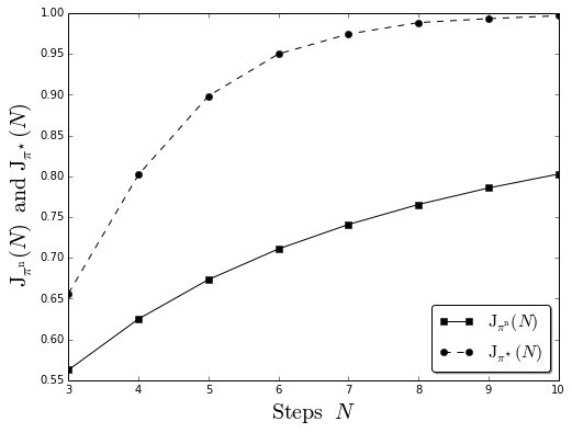
Figure 1: The probabilities of successfully reaching $|1\rangle$ from the initial state $|0\rangle$ using naive policy $\pi^{{\rm n}}$ and optimal feedback policy $\pi^{\star}$, respectively.

Moreover, as an illustration of the different actions between the naive and feedback strategies, we plot their policies for $N=5$ in Tables I and II, respectively.

$\pi^{\rm n}$	$k=0$	$k=1$	$k=2$	$k=3$	$k=4$
$|0\rangle$	$E_{1}$	$*$	$*$	$*$	$*$
$|1\rangle$	$*$	$*$	$*$	$*$	$*$
$|\phi_{1}\rangle$	$*$	$E_{2}$	$*$	$*$	$*$
$|\psi_{1}\rangle$	$*$	$E_{2}$	$*$	$*$	$*$
$|\phi_{2}\rangle$	$*$	$*$	$E_{3}$	$*$	$*$
$|\psi_{2}\rangle$	$*$	$*$	$E_{3}$	$*$	$*$
$|\phi_{3}\rangle$	$*$	$*$	$*$	$E_{4}$	$*$
$|\psi_{3}\rangle$	$*$	$*$	$*$	$E_{4}$	$*$
$|\phi_{4}\rangle$	$*$	$*$	$*$	$*$	$E_{5}$
$|\psi_{4}\rangle$	$*$	$*$	$*$	$*$	$E_{5}$

Table 1: The actions using naive strategy $\pi^{{\rm n}}$ to prepare the target state $|1\rangle$, starting from $|0\rangle$, for $N=5$. Here $E_{i}$ represents the measurement that the policy chooses, and $*$ means that it is not possible to be in that state at the corresponding step.

$\pi^{\star}$	$k=0$	$k=1$	$k=2$	$k=3$	$k=4$
$|0\rangle$	$E_{2}$	$E_{2}$	$E_{3}$	$E_{3}$	$E_{5}$
$|1\rangle$	$E_{5}$	$E_{5}$	$E_{5}$	$E_{5}$	$E_{5}$
$|\phi_{1}\rangle$	$E_{3}$	$E_{3}$	$E_{3}$	$E_{3}$	$E_{5}$
$|\psi_{1}\rangle$	$E_{5}$	$E_{5}$	$E_{5}$	$E_{5}$	$E_{5}$
$|\phi_{2}\rangle$	$E_{4}$	$E_{4}$	$E_{3}$	$E_{3}$	$E_{5}$
$|\psi_{2}\rangle$	$E_{1}$	$E_{1}$	$E_{1}$	$E_{1}$	$E_{5}$
$|\phi_{3}\rangle$	$E_{4}$	$E_{4}$	$E_{4}$	$E_{4}$	$E_{5}$
$|\psi_{3}\rangle$	$E_{1}$	$E_{1}$	$E_{2}$	$E_{2}$	$E_{5}$
$|\phi_{4}\rangle$	$E_{5}$	$E_{5}$	$E_{5}$	$E_{5}$	$E_{5}$
$|\psi_{4}\rangle$	$E_{2}$	$E_{2}$	$E_{2}$	$E_{2}$	$E_{5}$

Table 2: The actions using optimal feedback policy $\pi^{\star}$ to prepare the target state $|1\rangle$ for $N=5$.

2.3.2 Influence of Measurement Set

We now investigate how the size of the available measurement set $\mathcal{E}$ influences the successful arrival probability in $N$ steps under optimal feedback. In this case, the optimal arrival probability $\mathrm{J}_{\pi^{\star}}(N)$ is also a function of $T$, and we therefore rewrite $\mathrm{J}_{\pi^{\star}}(N)=\mathrm{J}_{\pi^{\star}}^{T}(N)$.

In Figure 2, we plot $\mathrm{J}_{\pi^{\star}}^{T}(N)$, for $T=10,100,1000$, respectively. The numerical results show that as $T$ increases, the $\mathrm{J}_{\pi^{\star}}^{T}(N)$ quickly tends to a limiting curve, suggesting the existence of some fundamental upper bound on the arrival probability in $N$ steps using sequential projections from an arbitrarily large measurement set.

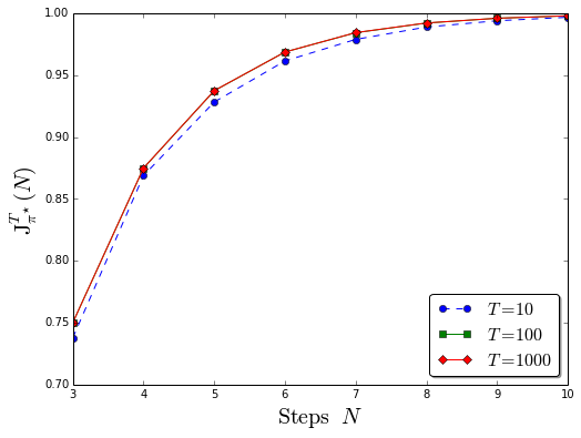
Figure 2: The probabilities of successfully reaching $|1\rangle$ from the initial state $|0\rangle$ using different sizes of measurement set by feedback strategy.

3 More Optimality Criteria

In this section, we discuss two other useful optimality criteria, to maximize the expected fidelity with the target state, or to minimize the expected time it takes to arrive at the target state.

3.1 Maximal Expected Fidelity

Given two density operators $\rho$ and $\sigma$, their fidelity is defined by [7]

$$F(\rho,\sigma)={\rm tr}\sqrt{\sqrt{\rho}\sigma\sqrt{\rho}}.$$

Fidelity measures the closeness of two quantum states. Now that our target state $|1\rangle\langle 1|$ is a pure state, we have

$${\rm tr}\sqrt{\sqrt{|1\rangle\langle 1|}\sigma\sqrt{|1\rangle\langle 1|}}=\sqrt{\langle 1|\sigma|1\rangle}.$$

Alternatively, we can consider the following objective functional

$$\tilde{\mathrm{J}}_{\pi}(N)=\mathbb{E}_{\pi}\Big{[}\langle 1|\rho_{{}_{N}}|1\rangle\Big{]},$$

and the goal is to find a policy that maximizes $\tilde{\mathrm{J}}_{\pi}(N)$.

For the two objective functionals ${\mathrm{J}}_{\pi}(N)$ and $\tilde{\mathrm{J}}_{\pi}(N)$, we denote their corresponding optimal policy as $\pi^{\star}(N)=\{\pi^{\star}_{k}(N)\}_{k=0}^{N-1}$ and $\pi^{\diamondsuit}(N)=\{\pi^{\diamondsuit}_{k}(N)\}_{k=0}^{N-1}$, respectively, where the time horizon $N$ is also indicated.

Let $\pi^{\diamondsuit}(N-1)\oplus E_{\ast}$ be the policy that follows $\pi^{\diamondsuit}(N-1)$ for $k=0,\dots,N-2$ and takes value $E_{\ast}$ for $k=N-1$. Let $\rho^{\rm u}_{k}$ be the unconditional density operator at step $k$ for $k=0,\dots,N-1$. The following equations hold:

$$\tilde{\mathrm{J}}_{\pi}(N-1) =\mathbb{E}_{\pi}\Big{[}\langle 1|\rho_{{}_{N-1}}|1\rangle\Big{]}$$ (5)

$$={\rm tr}\Big{(}\rho_{{}_{N-1}}^{\rm u}|1\rangle\langle 1|\Big{)}$$

$$=\mathbb{P}_{\pi^{\prime}}\Big{(}\rho_{{}_{N}}=|1\rangle\langle 1|\Big{)},$$

for any $\pi=\{\pi_{k}\}_{k=0}^{N-2}$, where $\pi^{\prime}=\pi\oplus E_{\ast}=\{\pi_{k}\}_{k=0}^{N-1}$ with $\pi_{N-1}=E_{\ast}$. As a result, the following relation holds between the optimal policies under the two objectives ${\mathrm{J}}_{\pi}(N)$ and $\tilde{\mathrm{J}}_{\pi}(N)$.

Proposition 2

It holds that $\max_{\pi}{\mathrm{J}}_{\pi}(N)=\max_{\pi}\tilde{\mathrm{J}}_{\pi}(N-1)$. In fact, $\pi^{\star}(N)=\pi^{\diamondsuit}(N-1)\oplus E_{\ast}$ with $E_{\ast}=\{|0\rangle\langle 0|,|1\rangle\langle 1|\}$.

The intuition behind Proposition 2 is that one would expect to get as closely as possible to the target state at step $N-1$, if one tends to successfully project onto the target state at step $N$. We also know from Proposition 2 that we can solve the maximal expected fidelity problem in $N$ steps by the solutions of maximizing the arrival probability in $N+1$ steps.

Similarly, we can also find the optimal policy $\pi^{\diamondsuit}$ for the objective $\tilde{\mathrm{J}}_{\pi}(N)$ using dynamical programming. Define the cost-to-go function $\tilde{\mathbf{V}}(k,x)$ for $\tilde{\mathrm{J}}_{\pi}(N)$ as

$$\tilde{\mathbf{V}}(k,x)=\max_{\pi}\mathbb{E}_{\pi}\Big{[}\langle 1|\rho_{{}_{N}}|1\rangle\ \Big{|}\ \rho_{k}=x\Big{]}$$ (6)

for $k=0,\dots,N$. Then $\tilde{\mathbf{V}}(k,x)$ satisfies the following recursive equation

$$\tilde{\mathbf{V}}(k,x)=\max_{u\in\mathcal{E}}\sum_{y\in\mathcal{Y}}\mathbb{P}\Big{(}y\Big{|}u,x\Big{)}\tilde{\mathbf{V}}\Big{(}k+1,\mathcal{M}_{u}^{y}(x)\Big{)},$$ (7)

for $k=0,\dots,N-1$, with terminal condition

$$\tilde{\mathbf{V}}(N,x)={\rm tr}\big{(}x|1\rangle\langle 1|\big{)}.$$ (8)

The optimal policy $\pi^{\diamondsuit}$ can be obtained by solving

$$\pi^{\diamondsuit}_{k}(\rho_{k})=\arg\max_{u\in\mathcal{E}}\sum_{y\in\mathcal{Y}}\mathbb{P}\Big{(}y\Big{|}u,\rho_{k}\Big{)}\tilde{\mathbf{V}}\Big{(}k+1,\mathcal{M}_{u}^{y}(\rho_{k})\Big{)}$$

for $k=0,\dots,N-1$. The maximal expected fidelity $\tilde{\mathrm{J}}_{\pi^{\diamondsuit}}(N)=\tilde{\mathbf{V}}(0,\rho_{0})$.

3.2 Minimal Arrival Time

In previous discussions the deadline $N$ plays an important role in the objective functionals as well as in their solutions. We now consider the case when the deadline is flexible, and we aim to minimize the average number of steps it takes to arrive at the target state. Now the control policy is denoted as $\pi=\{\pi_{k}\}_{k=0}^{\infty}$, where $\pi_{k}$ selects a measurement from the set $\mathcal{E}$. Associated with $\pi$, we define

$$\mathscr{A}_{\pi}:=\inf_{k}\Big{\{}\rho_{k}=|1\rangle\langle 1|\Big{\}}.$$ (9)

Note that $\mathscr{A}_{\pi}$ defines a stopping time (cf., [11]) associated with the random processes $\{\rho_{k}\}_{0}^{\infty}$, and we assume that $\pi$ is proper in the sense that

$$\mathbb{P}_{\pi}\Big{(}\mathscr{A}_{\pi}<\infty\Big{)}=1.$$

We continue to introduce

$$\mathrm{J}_{\pi}^{\flat}=\mathbb{E}_{\pi}\big{[}\mathscr{A}_{\pi}\big{]}$$ (10)

as the objective functional, which is the expected time it takes for the quantum state to reach the target $|1\rangle\langle 1|$ following policy $\pi$. Minimizing $\mathrm{J}_{\pi}^{\flat}$ is a stochastic shortest path problem [18].

We introduce $\mathscr{B}_{\pi}(x):=\inf_{k}\big{\{}\rho_{k}=|1\rangle\langle 1|\ \big{|}\ \rho_{0}=x\big{\}}$ and

$$\mathbf{V}^{\flat}(x)=\min_{\pi}\mathbb{E}_{\pi}\Big{[}\mathscr{B}_{\pi}(x)\Big{]}.$$ (11)

The Markovian property of $\{\rho_{k}\}_{k=0}^{\infty}$ leads to that the optimal policy $\pi^{\natural}$ is stationary in the sense that $\pi_{k}=\pi^{\natural}(x)$ for all $k$. The following conclusion holds applying directly the results of [18].

Proposition 3

The cost-to-go function $\mathbf{V}^{\flat}$ satisfies the following recursion

$$\mathbf{V}^{\flat}(x)=1+\min_{u\in\mathcal{E}}\sum_{y\in\mathcal{Y}}\mathbb{P}\Big{(}y\Big{|}u,x\Big{)}\mathbf{V}^{\flat}\Big{(}\mathcal{M}_{u}^{y}(x)\Big{)},$$ (12)

for all $x\neq|1\rangle\langle 1|$, with boundary condition $\mathbf{V}^{\flat}(|1\rangle\langle 1|)=0$. The optimal policy $\pi^{\natural}$ is given by

$$\pi^{\natural}(x)=\arg\min_{u\in\mathcal{E}}\sum_{y\in\mathcal{Y}}\mathbb{P}\Big{(}y\Big{|}u,x\Big{)}\mathbf{V}^{\flat}\Big{(}\mathcal{M}_{u}^{y}(x)\Big{)}.$$ (13)

The optimal $\mathrm{J}_{\pi^{\natural}}^{\flat}$ is given by $\mathrm{J}_{\pi^{\natural}}^{\flat}=\mathbf{V}^{\flat}(\rho_{0})$.

Technically it cannot be guaranteed that for any given measurement set $\mathcal{E}$, there always exists at least one policy $\pi$ under which $\mathrm{J}_{\pi}^{\flat}$ admits a finite number. However, some straightforward calculations indicate that for the set $\mathcal{E}$ of projective measurements given in Eq. (1), finite $\mathrm{J}_{\pi}^{\flat}$ can always be achieved for a class of policies.

$x$	$|0\rangle$	$|1\rangle$	$|\phi_{1}\rangle$	$|\psi_{1}\rangle$	$|\phi_{2}\rangle$	$|\psi_{2}\rangle$	$|\phi_{3}\rangle$	$|\psi_{3}\rangle$	$|\phi_{4}\rangle$	$|\psi_{4}\rangle$
$\pi^{\natural}(x)$	$E_{2}$	$E_{5}$	$E_{3}$	$E_{5}$	$E_{4}$	$E_{5}$	$E_{5}$	$E_{1}$	$E_{5}$	$E_{2}$

Table 3: The optimal policy $\pi^{\natural}$ minimizing the expected time it takes for the quantum state to reach the target state $|1\rangle\langle 1|$ for control set $\mathcal{E}_{\ast}$ with $T=5$.

3.3 Numerical Example: Minimal Arrival Time

Again, consider $T$ projective measurements from the set [17]

$$\mathcal{E}=\Big{\{}E_{i},\ \ i=1,2,\ldots,T\Big{\}}.$$

In Figure 3, we plot $\mathrm{J}_{\pi^{\natural}}^{\flat}(T)$ as a function of $T$, for $T=2,3,\ldots,30$. Numerical calculations show that the minimized average number of steps of driving $|0\rangle\langle 0|$ to $|1\rangle\langle 1|$ does not depend too much on the size of control set, it oscillates around $3.8$ for control sets of reasonable size. Also for measurement set $\mathcal{E}_{\ast}$ with $T=5$, we show the optimal policy $\pi^{\natural}$ in Table 3.

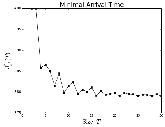
Figure 3: The minimized average number of steps it takes to arrive at the target state $|1\rangle\langle 1|$ from the initial state $|0\rangle\langle 0|$ employing control set $\mathcal{E}_{\ast}$ of size $T$.

4 Conclusions

We have proposed feedback designs for manipulating a quantum state to a target state by performing sequential measurements. Making use of Belavkin’s quantum feedback control theory, we showed that finding the measurement selection policy that maximizes the probability of successful state manipulation is an optimal control problem which can be solved by dynamical programming for any given set of measurements and a given time horizon. Numerical examples indicate that making use of feedback information significantly improves the success probability compared to classical scheme without taking feedback. It was shown that the probability of reaching the target state via feedback policy reaches $0.9968$ using merely $10$ steps, while classical results [16, 17] suggested that naive strategy via consecutive measurements in turn reaches success probability one when the number of steps tends to infinity. Maximizing the expected fidelity to the target state and minimizing the expected arrival time were also considered, and some connections and differences among these objectives were also discussed.

Acknowledgments

We gratefully acknowledge support by the Australian Research Council Centre of Excellence for Quantum Computation and Communication Technology (project number CE110001027), and AFOSR Grant FA2386-12-1-4075).

References

References

• [1] V. P. Belavkin, Towards control theory of quantum observable systems, Automatica and Remote Control, vol. 44, s188, 1983.
• [2] M. R. James, Risk-sensitive optimal control of quantum systems, Physical Review A, vol. 69, 032108, 2004.
• [3] L. Bouten, R. Van Handel, and M. R. James, A discrete invitation to quantum filtering and feedback control, SIAM Review, 51(2), 239-316, 2009.
• [4] S. J. Dolinar, An optimum receiver for the binary coherent state quantum channel, MIT Res. Lab. Electron. Quart. Progr. Rep., 111, pp. 115–120, 1973.
• [5] R. L. Cook, P. J. Martin, and J. M. Geremia, An optimum receiver for the binary coherent state quantum channel, Nature, vol. 446, pp.774–777, 2007.
• [6] C. W. Helstrom. Quantum Detection and Estimation Theory. Academic press, 1976.
• [7] M. A. Nielsen and I. L. Chuang. Quantum Computation and Quantum Information. Cambridge university press. 2010.
• [8] H. M. Wiseman, D. W. Berry, S. D. Bartlett, B. L. Higgins, and G. J. Pryde, Adaptive measurements in the optical quantum information laboratory, IEEE Journal of Selected Topics in Quantum Electronics, vol. 15, no. 6, pp. 1661–1672, 2009.
• [9] H. M. Wiseman and G. J. Milburn, Quantum theory of optical feedback via homodyne detection, Physical Review Letters, vol. 70, no. 5, 548, 1993.
• [10] M. L. Puterman. Markov Decision Processes: Discrete Stochastic Dynamic Programming. New York : Wiley, 1994.
• [11] R. Durrett. Probability: Theory and Examples, Duxbury advanced series, Third Edition, Thomson Brooks/Cole, 2005.
• [12] D. P. Bertsekas. Dynamic Programming and Optimal Control. Vol. II, 4th Edition. Athena Scientific, 2012.
• [13] S. Ashhab and F. Nori, Control-free control: manipulating a quantum system using only a limited set of measurements, Physical Review A, 82(6), 062103, 2010.
• [14] K. Jacobs, Feedback control using only quantum back-action, New Journal of Physics, 12(4), 043005, 2010.
• [15] H. M. Wiseman, Quantum control: Squinting at quantum systems, Nature, vol. 470, no. 7333, pp. 178–179, 2011.
• [16] L. Roa, M. L. de Guevara, A. Delgado, G. Olivares-Rentería, and A. Klimov, Quantum evolution by discrete measurements, Journal of Physics: Conference Series, vol. 84, 012017, 2007.
• [17] A. Pechen, N. Il’in, F. Shuang, and H. Rabitz, Quantum control by von neumann measurements, Physical Review A, vol. 74, no. 5, p. 052102, 2006.
• [18] D. P. Bertsekas and J. N. Tsitsiklis, An analysis of stochastic shortest path problems, Mathematics of Operations Research, 16(3), pp. 580–595, 1991.