Polymer Crowding and Shape Distributions in Polymer-Nanoparticle Mixtures

Abstract

Macromolecular crowding can influence polymer shapes, which is important for understanding the thermodynamic stability of polymer solutions and the structure and function of biopolymers (proteins, RNA, DNA) under confinement. We explore the influence of nanoparticle crowding on polymer shapes via Monte Carlo simulations and free-volume theory of a coarse-grained model of polymer-nanoparticle mixtures. Exploiting the geometry of random walks, we model polymer coils as effective penetrable ellipsoids, whose shapes fluctuate according to the probability distributions of the eigenvalues of the gyration tensor. Accounting for the entropic cost of a nanoparticle penetrating a larger polymer coil, we compute the crowding-induced shift in the shape distributions, radius of gyration, and asphericity of ideal polymers in a theta solvent. With increased nanoparticle crowding, we find that polymers become more compact (smaller, more spherical), in agreement with predictions of free-volume theory. Our approach can be easily extended to nonideal polymers in good solvents and used to model conformations of biopolymers in crowded environments.

I Introduction

Polymers are commonly confined within biological systems and other soft materials Minton (2001). Confinement can result from geometric boundaries, as in thin films and porous media, or from crowding by other species, as in nanocomposite materials and cellular environments. Within the nucleoplasm and cytoplasm of eukaryotic cells, for example, an assortment of macromolecules (proteins, RNA, DNA, etc.) share a tightly restricted space, occupying from 20% to 40% of the total volume van der Maarel (2008); Phillips et al. (2009). In this crowded milieu, smaller molecules exclude volume to larger, softer biopolymers, constraining conformations and influencing folding pathways. Macromolecular crowding, because of its profound influence on the structure, and hence function, of biopolymers, has been intensely studied over the past three decades Minton (1981, 2000, 2005); Ellis (2001); Richter et al. (2007, 2008); Elcock (2010); Hancock (2012); Denton (2013).

It is well established that crowding can significantly modify polymer conformations. The asymmetric shapes of folded and denatured states of biopolymers, in particular, are known to respond sensitively to the presence of crowding agents Goldenberg (2003); Dima and Thirumalai (2004); Cheung et al. (2005); Chen et al. (2012); Linhananta et al. (2012); Denesyuk and Thirumalai (2011, 2013). The shape distribution of a protein or RNA, for example, can vary with crowder concentration, which in turn, can affect the biopolymer’s function. Polymer shapes are also important in determining the nature of depletion-induced effective interactions between colloids and nanoparticles, thereby influencing thermodynamic stability of colloid-polymer mixtures against demixing. Direct measurements Lin et al. (2001) show, for example, that rodlike and spherical depletants induce significantly different interactions between colloids. Confinement and crowding effects are thus of practical concern for their impact on the properties of polymer-nanoparticle composite materials Nakatani et al. (2001); Kramer et al. (2005a, b, c); Balazs et al. (2006); Mackay et al. (2006); Nusser et al. (2010); Denton (2013) and for their role in diseases associated with protein aggregation Stradner et al. (2007).

Fundamental interest in polymer shapes dates to the dawn of polymer science. Already 80 years ago, Kuhn Kuhn (1934) recognized that macromolecules in solution are fluctuating objects, whose shapes are far from spherical, and that a linear polymer chain, when viewed in its principal-axis frame of reference, resembles a significantly elongated, flattened (bean-shaped) ellipsoid. The close analogy between polymers and random walks has inspired many mathematical and statistical mechanical studies to analyze sizes and shapes of random walks Fixman (1962); Flory and Fisk (1966); Flory (1969); Yamakawa (1970); Fujita and Norisuye (1970); Šolc (1971, 1973); Theodorou and Suter (1985); Rudnick and Gaspari (1986, 1987); Bishop and Saltiel (1988); Sciutto (1996); Murat and Kremer (1998); Eurich and Maass (2001). Such studies validate Kuhn’s insight and reveal broad distributions of radius of gyration and shape, as characterized by the eigenvalues of the gyration tensor.

In the case of colloidal particles larger than polymer radii of gyration (colloid limit), polymer depletion and induced effective attraction between colloids are relatively well understood phenomena Asakura and Oosawa (1954); Vrij (1976); Pusey (1991); Jones (2002); Fuchs and Schweizer (2002). The opposite case, in which smaller colloids (nanoparticles) can easily penetrate larger polymers (protein limit), has been studied more recently by theory Sear (1997, 2001, 2002), simulation Bolhuis et al. (2002, 2003); Moncho-Jordá et al. (2003); Cheung (2013), and experiment Hennequin et al. (2005); Zhang and van Duijneveldt (2006); Mutch et al. (2007). Previous studies, while analyzing depletion-induced interactions and demixing phase behavior, have not directly addressed the response of polymer shape to crowding. The purpose of this paper is to explore the influence of nanoparticle crowding on the shapes of polymers in polymer-nanoparticle mixtures.

In the next section, we define our model of a polymer-nanoparticle mixture. In Sec. III, we describe our simulation method and outline the free-volume theory, relegating details to an appendix. In Sec. IV, we present results from our simulations for the shape distributions of crowded polymers and compare with theoretical predictions. Finally, in Sec. V, we summarize and suggest possible extensions of our approach for future work.

II Models

II.1 Polymer-Nanoparticle Mixtures

We model a mixture of nanoparticles and nonadsorbing polymers using a generalization of the Asakura-Oosawa-Vrij (AOV) model of colloid-polymer mixtures Asakura and Oosawa (1954); Vrij (1976). The original AOV model represents the particles as hard (impenetrable) spheres, interacting via a hard-sphere pair potential,

$$v_{nn}(r) = \left\{\begin{array}[]{l@{\quad\quad}l}\infty~{},&r<2R_{n}~{},\\[4.30554pt] 0~{},&r\geq 2R_{n}~{},\end{array}\right.$$ (3)

and the polymers as effective spheres of fixed size (radius of gyration) that are mutually ideal (noninteracting), but impenetrable to the particles. While the neglect of polymer-polymer interactions is justified for polymers in a theta solvent de Gennes (1979), the effective-sphere approximation ignores aspherical conformations and shape fluctuations of polymer coils. Moreover, the assumption of hard polymer-particle interactions is physically reasonable only for particles much larger than the polymers. In order to study the influence of nanoparticle crowding on polymer shapes, we generalize the AOV model by allowing nanoparticles to penetrate polymers and by representing the polymers as ellipsoids that fluctuate in size and shape.

Figure 1: Model of polymer-nanoparticle mixtures. Polymers are penetrable ellipsoids that can fluctuate in size and shape. Nanoparticles are hard spheres of fixed size.

Following Schmidt and Fuchs Schmidt and Fuchs (2002), we attribute to each overlapping polymer-nanoparticle pair, an average free energy cost $\varepsilon$, which accounts for the loss in conformational entropy of the coil. For a hard sphere penetrating an ideal polymer coil, in a theta solvent at temperature $T$, polymer field theory predicts $\varepsilon=3k_{B}T/q$, where $q=R_{p}/R_{n}$ is the ratio of the polymer radius of gyration $R_{p}$ to the nanoparticle radius $R_{n}$ Eisenriegler et al. (1996); Hanke et al. (1999). An obvious refinement of this model would allow the overlap free energy to vary with the nanoparticle’s position relative to the polymer center. Such effective interaction energy profiles have been computed from Monte Carlo simulations of polymers on a lattice Pelissetto and Hansen (2006). Alternatively, the overlap free energy profile could be derived from an approximation for the monomer density in the ellipsoidal polymer model Eurich and Maass (2001) (see below). In the current study, however, for conceptual simplicity and computational efficiency, we neglect this level of spatial resolution. Furthermore, since the nanoparticles in our model are chemically inert and act only to limit the free volume available to the polymers, we assume that the theta temperature of the solution is independent of nanoparticle concentration.

II.2 Penetrable Polymer Model

The size and shape of a polymer coil can be characterized by the gyration tensor, defined by

$${\bf T}~{}=~{}\frac{1}{N}\sum_{i=1}^{N}{\bf r}_{i}~{}{\bf r}_{i}~{},$$ (4)

where ${\bf r}_{i}$ denotes the position of the $i^{\rm th}$ of $N$ segments, relative to the center of mass. Any particular conformation has a radius of gyration defined by

$$R_{p}=\left(\frac{1}{N}\sum_{i=1}^{N}r_{i}^{2}\right)^{1/2}=\sqrt{\Lambda_{1}+\Lambda_{2}+\Lambda_{3}}~{},$$ (5)

where $\Lambda_{1}$, $\Lambda_{2}$, $\Lambda_{3}$ are the eigenvalues of ${\bf T}$. For reference, the gyration tensor is related to the moment of inertia tensor ${\bf I}$, familiar from classical mechanics of rigid bodies, via ${\bf T}=R_{p}^{2}{\bf 1}-{\bf I}$, where ${\bf 1}$ is the unit tensor. The root-mean-square (rms) radius of gyration, which is experimentally measurable, is given by

$$R_{g}=\sqrt{\left\langle R_{p}^{2}\right\rangle}=\sqrt{\left\langle\Lambda_{1}+\Lambda_{2}+\Lambda_{3}\right\rangle}~{},$$ (6)

where the angular brackets represent an ensemble average over conformations.

Now, if the average in Eq. (6) is defined relative to a fixed (laboratory) frame of reference, then the average tensor is symmetric, has equal eigenvalues, and describes a sphere. If instead the average is performed in a frame of reference that rotates with the polymer’s principal axes, the coordinate axes being labelled to preserve the order of the eigenvalues by magnitude ($\Lambda_{1}>\Lambda_{2}>\Lambda_{3}$), then the average tensor is asymmetric and describes an anisotropic object Rudnick and Gaspari (1986, 1987). In other words, viewed from the laboratory frame, the average shape of a random walk is spherical, but viewed from the principal-axis frame, the average shape is aspherical Kuhn (1934). In fact, in the principal-axis frame, the average shape is a significantly elongated (prolate), flattened ellipsoid with principal radii along the three independent axes in the approximate ratio 3.4 : 1.6 : 1 Kuhn (1934); Šolc (1971, 1973). Each eigenvalue of the gyration tensor is proportional to the square of the respective principal radius of the general ellipsoid that best fits the shape of the polymer, an arbitrary point $(x,y,z)$ on the surface of the ellipsoid satisfying

$$\frac{x^{2}}{\Lambda_{1}}+\frac{y^{2}}{\Lambda_{2}}+\frac{z^{2}}{\Lambda_{3}}=3~{}.$$ (7)

This ellipsoid serves as a gross representation of the tertiary structure of a biopolymer.

The shape of an ideal, freely-jointed polymer coil of $N$ segments of length $l$, modeled as a soft Gaussian ellipsoid Murat and Kremer (1998), has a normalized probability distribution that is well approximated by the analytical ansatz of Eurich and Maass Eurich and Maass (2001):

$$P_{r}(\lambda_{1},\lambda_{2},\lambda_{3})=\prod_{i=1}^{3}P_{ir}(\lambda_{i})~{},$$ (8)

where $\lambda_{i}\equiv\Lambda_{i}/(Nl^{2})$ are scaled (dimensionless) eigenvalues and

$$P_{ir}(\lambda_{i})=\frac{(a_{i}d_{i})^{n_{i}-1}\lambda_{i}^{-n_{i}}}{2K_{i}}\exp\left(-\frac{\lambda_{i}}{a_{i}}-d_{i}^{2}\frac{a_{i}}{\lambda_{i}}\right)~{},$$ (9)

with fitting parameters $K_{1}=0.094551$, $K_{2}=0.0144146$, $K_{3}=0.0052767$, $a_{1}=0.08065$, $a_{2}=0.01813$, $a_{3}=0.006031$, $d_{1}=1.096$, $d_{2}=1.998$, $d_{3}=2.684$, $n_{1}=1/2$, $n_{2}=5/2$, and $n_{3}=4$. The assumption of independent eigenvalues underlying the factorization ansatz of Eq. (8) is not exact, since an extension of a random walk in one direction affects the probability of an extension in an orthogonal direction. Nevertheless, conformations that significantly violate the ansatz are rare for random walks sufficiently long to model real polymers. It should be noted that the ellipsoidal polymer model has also been extended to block copolymers Eurich et al. (2007).

In modeling mixtures of polymers and nanoparticles, it is convenient to consider the system to be in osmotic equilibrium with a reservoir of pure polymer, which fixes the polymer chemical potential. A key parameter that defines the system is the ratio, $q_{r}\equiv R_{g}^{r}/R_{n}$, of the rms radius of gyration of polymer in the reservoir $R_{g}^{r}$ to the nanoparticle radius. Expressed in terms of the scaled eigenvalues, the ratio of the rms radius of gyration in the system [Eq. (6)] to its counterpart in the reservoir [$R_{g}^{r}=l\sqrt{N/6}$] is given by

$$\frac{R_{g}}{R_{g}^{r}}=\sqrt{6\left\langle\lambda_{1}+\lambda_{2}+\lambda_{3}\right\rangle}~{}.$$ (10)

Similarly, the principal radii are related to the scaled eigenvalues according to

$$R_{i}=R_{g}^{r}\sqrt{18\lambda_{i}}~{},\quad i=1,2,3~{}.$$ (11)

The broad eigenvalue distributions described by Eq. (9) imply significant fluctuations in size ($R_{g}$) and shape ($\lambda_{i}$) of the polymer [see Fig. (3) below]. The deviation of a polymer’s average shape from a perfect sphere can be quantified by an asphericity parameter Rudnick and Gaspari (1986, 1987)

$$A=1-3\frac{\left\langle\lambda_{1}\lambda_{2}+\lambda_{1}\lambda_{3}+\lambda_{2}\lambda_{3}\right\rangle}{\left\langle(\lambda_{1}+\lambda_{2}+\lambda_{3})^{2}\right\rangle}~{}.$$ (12)

By this definition, a spherical object with all eigenvalues equal has $A=0$, while an elongated object, with one eigenvalue much larger than the other two, has $A\simeq 1$. In the next section, we describe computational methods for calculating the shape distribution, radius of gyration, and asphericity of polymers crowded by nanoparticles.

III Computational Methods

III.1 Monte Carlo Simulations

To explore the influence of nanoparticle crowding on polymer conformations, we have developed a Monte Carlo (MC) method for simulating mixtures of hard nanoparticles and ideal polymers, whose uncrowded shape distribution follows Eq. (9). In the canonical ensemble, the temperature, particle numbers ($N_{n}$ nanoparticles, $N_{p}$ polymers), and volume $V$ are fixed. Trial moves include displacements of nanoparticles and, for the polymers, displacements, rotations, and shape changes. In the standard Metropolis algorithm Binder (1995); Frenkel and Smit (2001); Binder and Heermann (2010), a trial move from an old to a new configuration, due to displacement of any particle or rotation of a polymer, is accepted with probability

$${\cal P}_{\rm config}({\rm old}\to{\rm new})=\min\left\{\exp(-\beta\Delta U),~{}1\right\}~{},$$ (13)

where $\beta=1/(k_{B}T)$ and $\Delta U$ is the associated change in potential energy.

Overlaps of hard-sphere nanoparticles are easily detected and are, of course, automatically rejected. Polymer-nanoparticle overlaps, on the other hand, are harder to identify, because of the nontrivial calculation required to determine the shortest distance between the surface of a sphere and that of a general ellipsoid Frenkel and Mulder (1985). To avoid the computational overhead of this calculation, we here restrict our investigations to cases in which the nanoparticles are much smaller than the rms radius of gyration of the polymers ($q_{r}\gg 1$). In this limit, we can accurately approximate the volume excluded by a polymer to a nanoparticle, whose true shape is an ellipsoid coated by a shell of uniform thickness $R_{n}$, by a larger ellipsoid, whose principal radii are extended by $R_{n}$. Thus, we approximate the overlap criterion by

$$\left(\frac{x}{\sqrt{\Lambda_{1}}+R_{n}}\right)^{2}+\left(\frac{y}{\sqrt{\Lambda_{2}}+R_{n}}\right)^{2}+\left(\frac{z}{\sqrt{\Lambda_{3}}+R_{n}}\right)^{2}<1~{},$$ (14)

where $(x,y,z)$ here represent the coordinates of the vector joining the centers of the sphere and ellipsoid.

In the event that a trial move results in a change in the number $\Delta N_{pn}$ of polymer-nanoparticle overlaps, then $\Delta U=\varepsilon\Delta N_{pn}$. Thus, any displacement or rotation that reduces, or leaves unchanged, the number of overlaps is automatically accepted, while a move that creates new overlaps is accepted only with a probability equal to the Boltzmann factor for $\Delta U$. For trial rotations, we define the orientation of a polymer by a unit vector ${\bf u}$, aligned with the long ($\lambda_{1}$) axis of the ellipsoid at polar angle $\theta$ and azimuthal angle $\phi$, and generate a new (trial) direction ${\bf u}^{\prime}$ via

$${\bf u}^{\prime}=\frac{{\bf u}+\tau{\bf v}}{|{\bf u}+\tau{\bf v}|}~{},$$ (15)

where ${\bf v}$ is a unit vector with random orientation and $\tau$ is a tolerance that determines the magnitude of the trial rotation Frenkel and Smit (2001). To confirm even sampling of orientations, we checked that histograms of $\cos\theta$ and $\phi$ for a free (i.e., uncrowded) polymer were flat.

A trial change in shape of an ellipsoidal polymer coil, from an old shape $\lambda_{\rm old}$ to a new shape $\lambda_{\rm new}=\lambda_{\rm old}+\Delta\lambda$, is accepted with probability

$${\cal P}_{\rm shape}(\lambda_{\rm old}\to\lambda_{\rm new})=\min\left\{\frac{P_{r}(\lambda_{\rm new})}{P_{r}(\lambda_{\rm old})}e^{-\beta\Delta U},~{}1\right\}~{},$$ (16)

where $\lambda\equiv(\lambda_{1},\lambda_{2},\lambda_{3})$ collectively denotes the eigenvalues and $P_{r}(\lambda)$ is the reservoir polymer shape distribution [Eqs. (8) and (9)]. Thus, a trial shape change is accepted with a probability equal to the Boltzmann factor for the change in potential energy multiplied by the ratio of the new to the old shape probabilities. Through trial changes in gyration tensor eigenvalues, a polymer explores the landscape of possible shapes in the presence of crowders and evolves toward a new equilibrium shape distribution.

One MC step of a simulation consists of a trial displacement of every nanoparticle, followed by a trial displacement, rotation, and shape change of every polymer. To maximize computational efficiency, we chose tolerances of $0.01~{}\sigma_{n}$ for trial displacements, $\tau=0.001$ for trial rotations, and for trial shape (eigenvalue) changes, $\Delta\lambda_{1}=0.01$, $\Delta\lambda_{2}=0.003$, and $\Delta\lambda_{3}=0.001$. To facilitate extensions and portability of our simulation methods, we coded our MC algorithm in the Java programming language within the Open Source Physics library Gould et al. (2006); Christian (2006), exploiting the numerical and visualization classes of the library. The simulations thus run on any platform, with a convenient graphical user interface, and so may have both scientific and pedagogical value.

III.2 Free-Volume Theory of Crowding

For the model polymer-nanoparticle mixtures described in Sec. II, Denton et al.  Denton et al. recently developed a free-volume theory, which generalizes the theory of Lekkerkerker et al.  Lekkerkerker et al. (1992) from incompressible, spherical polymers to compressible, aspherical polymers. To guide our choice of parameters, check for consistency, and test the theory, we compare our simulation results with theoretical predictions. As outlined in Appendix A, the theory predicts a crowded-polymer shape probability distribution of the form

$$P(\lambda;\phi_{n})=P_{r}(\lambda)\frac{\alpha(\lambda;\phi_{n})}{\alpha_{\rm eff}(\phi_{n})}~{},$$ (17)

where the free-volume fraction $\alpha(\lambda;\phi_{n})$ is the fraction of the total volume accessible to a polymer, whose ellipsoidal shape is characterized by the eigenvalues $\lambda=(\lambda_{1},\lambda_{2},\lambda_{3})$, amidst nanoparticles of volume fraction $\phi_{n}=n_{n}(4\pi/3)R_{n}^{3}$ (number density $n_{n}$), and

$$\alpha_{\rm eff}(\phi_{n})\equiv\int{\rm d}\lambda\,P_{r}(\lambda)\alpha(\lambda;\phi_{n})$$ (18)

is an effective polymer free-volume fraction, expressed as an average of $\alpha(\lambda;\phi_{n})$ over polymer shapes in the reservoir. In practice, we adopt the ansatz for $P_{r}(\lambda)$ described in Sec. II.2 and compute $\alpha(\lambda;\phi_{n})$ by implementing the generalized scaled-particle theory of Oversteegen and Roth Oversteegen and Roth (2005). From Eq. (17), the probability distribution for a single eigenvalue is obtained by integrating over the other two eigenvalues. For example,

$$P_{1}(\lambda_{1};\phi_{n})=\int_{0}^{\infty}d\lambda_{2}\,\int_{0}^{\infty}d\lambda_{3}\,P(\lambda;\phi_{n})~{}.$$ (19)

In calculating the rms radius of gyration [Eq. (10)] and asphericity [Eq. (12)], mean values of functions of eigenvalues $f(\lambda)$ are defined as averages with respect to $P(\lambda)$:

$$\left\langle f\right\rangle=\int d\lambda\,P(\lambda)f(\lambda)~{}.$$ (20)

In the next section, we present numerical results from MC simulations and free-volume theory that characterize the shapes of ideal polymers in crowded environments.

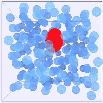
Figure 2: Snapshot of a simulation of $N_{n}=216$ nanoparticles (blue spheres) and one polymer (red ellipsoid) in a cubic box. The polymer rms radius of gyration in the reservoir equals five times the nanoparticle radius ($q_{r}=5$).

Figure 3: Probability distributions for the eigenvalues (a) $\lambda_{1}$, (b) $\lambda_{2}$, and (c) $\lambda_{3}$ of the gyration tensor of a polymer coil, modeled as an ideal, freely-jointed chain. Monte Carlo simulation data (symbols) are compared with predictions of free-volume theory (solid curves) for a single ellipsoidal polymer, with rms radius of gyration in the reservoir equal to five times the nanoparticle radius ($q_{r}=5$), amidst $N_{n}=216$ nanoparticles with volume fraction $\phi_{n}=0.1$ (triangles), 0.2 (squares), and 0.3 (circles). Also shown are the reservoir distributions (dashed curves), in the absence of nanoparticles ($\phi_{n}=0$).

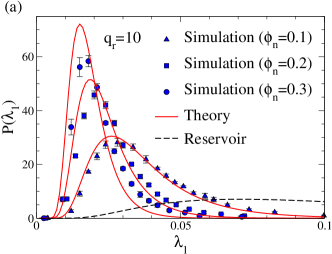
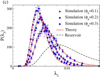
Figure 4: Same as Fig. 3, but for larger polymer ($q_{r}=10$). Notice the changes in scale.

Figure 5: Root-mean-square radius of gyration of a polymer vs. nanoparticle volume fraction [Eq. (10)]. Monte Carlo simulation data (symbols) are compared with predictions of free-volume theory for ellipsoidal polymer (solid curves) and spherical polymer (dashed curves). Results are shown for reservoir polymer-to-nanoparticle size ratio $q_{r}=5$ (circles), $q_{r}=10$ (squares). (Error bars are smaller than symbols.)

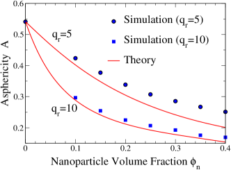
Figure 6: Asphericity of an ellipsoidal polymer vs. nanoparticle volume fraction [Eq. (12)]. Monte Carlo simulation data (symbols) are compared with predictions of free-volume theory (curves). Results are shown for reservoir polymer-to-nanoparticle size ratio $q_{r}=5$ (circles) and $q_{r}=10$ (squares). (Error bars are smaller than symbols.) As crowding increases, the polymer becomes more compact (less aspherical).

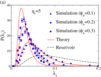
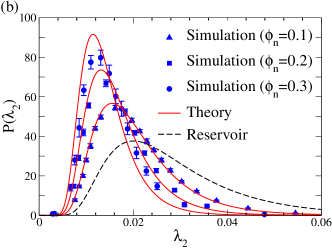
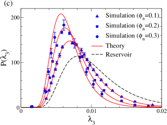
Figure 7: Same as Fig. 3, but for higher polymer concentration ($N_{p}=8$, $\phi_{p}\simeq 0.5$).

IV Results and Discussion

To investigate how the shapes of ideal polymers respond to crowding, we simulated compressible, penetrable polymers, immersed in a fluid of smaller, hard-sphere nanoparticles (protein limit), modeled as described in Sec. II, and using the MC method outlined in Sec. III.1. Confining the system to a cubic box of fixed size with periodic boundary conditions applied to opposite faces, we initialized the nanoparticles on the sites of a cubic lattice and the polymers at interstitial sites. For illustration, a snapshot of the simulation cell is shown in Fig. 2.

Each run consisted of an initial equilibration stage of $5\times 10^{4}$ MC steps, followed by a data collection stage of $10^{7}$ steps. We monitored the total overlap energy and shape distributions and confirmed that the averages of these diagnostics were stable after the equilibration stage. Our results represent averages over $10^{4}$ independent configurations (spaced by intervals of $10^{3}$ steps) from each of five independent runs (total of $5\times 10^{4}$ configurations), with statistical uncertainties computed from standard deviations of the five runs. Most of our simulations were performed for systems of $N_{n}=216$ nanoparticles. To rule out finite-size effects, however, we repeated several runs for larger systems (up to $N_{n}=1728$) and confirmed that the results are independent of system size to within statistical fluctuations.

Figure 3 shows the probability distributions for the eigenvalues of the gyration tensor, representing the shape of the best-fit ellipsoid, for one polymer amidst $N_{n}=216$ nanoparticles, with the reservoir rms radius of gyration equal to five times the nanoparticle radius ($q_{r}=5$). At this large size ratio, our approximation for the polymer-nanoparticle overlap criterion [Eq. (14)] is quite accurate. With increasing nanoparticle volume fraction, from $\phi_{n}=0$ (reservoir) to $\phi_{n}=0.3$, the shape distributions progressively shift toward smaller eigenvalues, reflecting compression of the polymer along all three principle axes. The greatest fractional shift occurs, however, in the two largest eigenvalues ($\lambda_{1}$ and $\lambda_{2}$), implying that the best-fit ellipsoids tend to become less elongated.

Figure 4 shows the probability distributions for a polymer twice as large ($q_{r}=10$). Doubling the size ratio, while still avoiding significant finite-size effects, required doubling the simulation box length, and thus increasing eight-fold the number of nanoparticles ($N_{n}=1728$). As a rough guide, the simulation box must be large enough that the long axis of the polymer cannot span a significant fraction of the box length. Otherwise, correlations between a polymer and its own images can cause spurious effects. To minimize computational time for the larger system, we reduced the run length to $10^{6}$ MC steps, without a significant change in results. Our runs of $10^{7}$ steps proved, therefore, to be conservatively long.

For the same nanoparticle concentration, the shape distributions of the larger polymer are considerably more shifted relative to the reservoir distributions. This trend is easily explained by considering the average free energy cost $\bar{E}_{pn}$ of polymer-nanoparticle overlaps. Neglecting correlations, the average number of overlaps scales as $\phi_{n}q^{3}$, while the penetration energy scales as $q^{-1}$. Thus, the average overlap energy scales as $\bar{E}_{pn}\sim\phi_{n}q^{2}$, i.e., the crowding effect increases with the square of the size ratio.

Also shown in Figs. 3 and 4 are the shape distributions predicted by the free-volume theory, described in Sec. III.2 and the Appendix. In this limit of dilute polymer concentration, theory and simulation are evidently in close agreement at lower nanoparticle concentrations. As the polymer becomes increasingly crowded, however, slight quantitative deviations emerge, particularly for the largest eigenvalue $\lambda_{1}$ of the gyration tensor at $q_{r}=5$. These small deviations result from the mean-field theory’s neglect of polymer-nanoparticle correlations and from approximations inherent in scaled-particle theory.

From the polymer shape (eigenvalue) distributions, we have computed the rms radius of gyration [Eq. (10)] and asphericity [Eq. (12)] of a single crowded polymer as functions of nanoparticle concentration. As shown in Figs. 5 and 6, an ideal polymer responds to crowding by contracting in size (decreasing $R_{g}$) and becoming more spherical in shape (decreasing $A$). Thus, with increasing nanoparticle volume fraction, the polymer progressively compactifies. Increasing the size ratio from $q_{r}=5$ to $q_{r}=10$ enhances the crowding effect, for reasons explained above, the polymer becoming even smaller and more spherical for a given nanoparticle concentration.

Figures 5 and 6 also show that the free-volume theory again accurately captures the trends in size and shape. Nevertheless, small gaps between theory and simulation are apparent, and these quantitative deviations grow with increasing nanoparticle concentration. The theory’s slight, but consistent, underprediction of both $R_{g}$ and $A$ is due mainly to the underprediction of $\lambda_{1}$. To emphasize the distinction between ellipsoidal and spherical polymer models, Fig. 5 also shows, for comparison, free-volume theory predictions for a spherical, compressible polymer model Denton and Schmidt (2002); Lu and Denton (2011). Clearly ellipsoidal polymers, being free to distort their shape, have significantly larger radii of gyration in crowded environments than polymers that are constrained to remain spherical.

To explore crowding at higher polymer concentrations, we increased the polymer volume fraction to $\phi_{p}\equiv n_{p}(4\pi/3)(R_{g}^{r})^{3}\simeq 0.5$, with $N_{p}=8$ polymers now sharing the simulation box with $N_{n}=216$ nanoparticles at size ratio $q_{r}=5$. These conditions actually place the system in a part of the phase diagram that is thermodynamically unstable toward polymer-nanoparticle demixing Moncho-Jordá et al. (2003); Zhang and van Duijneveldt (2006). Bulk phase separation is prevented only by the constraints of the NVT ensemble and the relatively small system size. As illustrated in Fig. 7, the simulated shape distributions do not substantially differ from those for a single polymer (Fig. 3). Interestingly, this behavior differs from that observed in simulations of the spherical, compressible, ideal polymer model Lu and Denton (2011) in the colloid limit ($q_{r}=1$), where polymer compression reversed with increasing crowding. This reversal, caused by polymer clustering and shielding – a correlation effect neglected by the mean-field free-volume theory – is not observed here in the protein limit.

In closing this section, we briefly discuss the relation of our approach to experiments and other modeling approaches. Recent studies that applied small-angle neutron scattering to polystyrene chains in the presence of various molecular crowding agents Kramer et al. (2005a, b, c), and to deuterated PEG amidst the polysaccharide crowder Ficoll 70 Le Coeur et al. (2009, 2010), reported substantial crowding-induced polymer compression. Although the polymers in these experiments were nonideal and relatively close in size to the crowders, our results for ideal polymers and larger size ratios are at least qualitatively consistent with these observations.

The role of crowding in native-denatured transitions of real polypeptides was recently modeled by Minton Minton (2005). Applying an effective two-state model of proteins Minton (2000), Minton calculated excluded-volume interactions between unfolded proteins and macromolecular cosolutes, modeled as hard spheres or rods. Taking as input the radius of gyration probability distributions of four real proteins, computed by Goldenberg Goldenberg (2003) via Monte Carlo simulations that include steric interactions between nonadjacent amino acid residues, Minton calculated chemical potentials and radii of gyration of unfolded proteins as a function of cosolute concentration. He concluded that long-range intramolecular steric interactions significantly increase the radii of gyration of unfolded polypeptides in crowded environments. Our approach can potentially complement Minton’s by incorporating knowledge of both the size and shape of the uncrowded polymer.

V Conclusions

In summary, we have investigated the influence of crowding on polymer shapes in a coarse-grained model of polymer-nanoparticle mixtures. The ideal polymer coils are modeled here as effective ellipsoids that fluctuate in shape according to the probability distributions of the eigenvalues of the gyration tensor of a random walk. The nanoparticles are modeled as hard spheres that can penetrate the polymers with a free energy penalty varying inversely with the polymer-to-nanoparticle size ratio $q_{r}$. For this model, we performed both Monte Carlo simulations, incorporating novel trial moves that change the polymer shape, and free-volume theory calculations. In the protein limit, for size ratios of $q_{r}=5$ and 10, we computed the shape distributions, radius of gyration, and asphericity of ideal polymers induced by crowding of hard-sphere nanoparticles. Relative to uncrowded polymers, we observed significant shifts in polymer shape, which grow with increasing nanoparticle concentration and size ratio. Our results demonstrate that ideal polymers become more compact when crowded by smaller, hard nanoparticles, in good agreement with predictions of free-volume theory. The methods and results presented here significantly extend the scope of previous studies of colloid-polymer mixtures in which the polymers were modeled as compressible spheres Denton and Schmidt (2002); Lu and Denton (2011).

For future work, we envision several intriguing directions in which our approach may be extended. While the present paper focuses on the influence of nanoparticles on polymers, one could, conversely, study the impact of polymers on effective interactions between nanoparticles. In particular, by simulating a pair of nanoparticles in a bath of shape-fluctuating polymers, the depletion-induced potential of mean force between nanoparticles could be computed and compared with simulations of more microscopic models Bolhuis et al. (2003), as well as with predictions of polymer field theory Eisenriegler et al. (2003) and density-functional theory Forsman and Woodward (2009); Wang et al. (2014), in the protein limit.

Our model can be refined by replacing the step-function polymer-nanoparticle overlap energy profile with a more realistic, continuous profile based on the monomer density profile Eurich and Maass (2001) or on molecular simulations Pelissetto and Hansen (2006). Furthermore, by replacing the shape distribution of an ideal (non-self-avoiding) random walk with that of a nonideal (self-avoiding) walk Lhuilier (1988); Sciutto (1996); Schäfer (1999), the model can be extended from ideal polymers in theta solvents to real polymers in good solvents. Such extensions can include biopolymers in aqueous solutions, such as unfolded proteins, whose persistence lengths can be sensitive to excluded-volume interactions Minton (2005), and whose uncrowded size distributions can be independently computed Goldenberg (2003). For a single biopolymer in a crowded environment, our computational methods can be directly applied, given as input the requisite shape distribution Denesyuk and Thirumalai (2011); Kudlay et al. (2012); Denesyuk and Thirumalai (2013). Simulating solutions of multiple self-avoiding polymers would require incorporating polymer-polymer interactions Frenkel and Mulder (1985); Allen et al. (1993). It is important to note, however, that our Monte Carlo approach, while efficiently sampling polymer conformations, does not accurately represent time scales for distinct molecular motions – diffusion, rotation, and shape fluctuations. Therefore, our methods, while finding equilibrium shapes of crowded polymers, cannot describe dynamical processes, such as folding and unfolding.

Beyond adding realism to the polymer model, our approach can also be extended to mixtures of polymers with nonspherical Kudlay et al. (2012) or charged Denton and Schmidt (2005); Fortini et al. (2005) crowders, or to other crowded environments, such as confinement within a vesicle Fošnarič et al. (2013), or two-dimensional confinement, e.g., of DNA adsorbed onto lipid membranes Fang and Yang (1997); Maier and Rädler (2000). Finally, for all of these systems, it would be interesting to explore the influence of polymer shape degrees of freedom on bulk thermodynamic properties, including the demixing transition between polymer-rich and polymer-poor phases, by implementing our Monte Carlo methods in either the Gibbs ensemble Lu and Denton (2011) or the grand canonical ensemble Vink and Horbach (2004a, b).

Appendix A Free-Volume Theory

Here, we outline in greater detail the theory sketched in Sec. III.2. In the semi-grand ensemble, a fixed number $N_{n}$ of nanoparticles are confined to a volume $V$, while the polymers can exchange with a reservoir of polymer that maintains constant polymer chemical potential $\mu_{p}$ in the system. At a given temperature, the thermodynamic state is characterized by the nanoparticle number density, $n_{n}=N_{n}/V$, and the polymer number density in the reservoir, $n_{p}^{r}\propto\exp(\beta\mu_{p})$ (ideal polymer). The polymer number density in the system, $n_{p}=N_{p}/V$, which depends on the nanoparticle density, is determined by chemical equilibrium between the system and reservoir.

The free-volume theory, a generalization of the theory first proposed by Lekkerkerker et al.  Lekkerkerker et al. (1992) for the AOV model of colloid-polymer mixtures, can be derived by separating the Helmholtz free energy density, $f=f_{\rm id}+f_{\rm ex}$, into an ideal-gas contribution $f_{\rm id}$ and an excess contribution $f_{\rm ex}$ due to interparticle interactions. The excess free energy density consists of a hard-sphere nanoparticle contribution $f_{\rm hs}(\phi_{n})$ and a polymer contribution $f_{p}$, which depends on polymer-nanoparticle interactions. In a mean-field approximation, the polymer excess free energy density is equated to that of ideal polymers confined to the free volume (not excluded by the nanoparticles).

For shape-fluctuating polymers, the free energy must be averaged over shape degrees of freedom and supplemented by a conformational free energy. Assuming that a polymer of a given shape (i.e., eigenvalues $\lambda$) has the same conformational entropy in the system as in the reservoir, namely $k_{B}\ln P_{r}(\lambda)$, the polymer excess free energy density is approximated by

$$\beta f_{p}(\phi_{n},\phi_{p})=-n_{p}\int{\rm d}\lambda\,P(\lambda;\phi_{n})\ln[P_{r}(\lambda)\alpha(\lambda;\phi_{n})]~{},$$ (21)

where $P(\lambda;\phi_{n})$ and $\alpha(\lambda;\phi_{n})$ are the probability distribution and free-volume fraction, respectively, of polymer coils of shape $\lambda$ amidst nanoparticles of volume fraction $\phi_{n}\equiv(4\pi/3)n_{n}R_{n}^{3}$. The ideal-gas free energy density is given exactly by

$$\beta f_{\rm id}(\phi_{n},\phi_{p}) = n_{p}\int{\rm d}\lambda\,P(\lambda;\phi_{n})\{\ln[\phi_{p}P(\lambda;\phi_{n})]-1\}$$ (22)

$$+ n_{n}\left(\ln\phi_{n}-1\right)~{},$$

where $\phi_{p}\equiv(4\pi/3)n_{p}(R_{g}^{r})^{3}$ is the effective polymer volume fraction in the system and $R_{g}^{r}$ is the rms radius of gyration in the reservoir.

Equating chemical potentials of ideal polymers of a given shape in the system and reservoir now implies

$$n_{p}(\phi_{n})P(\lambda;\phi_{n})=n_{p}^{r}P_{r}(\lambda)\alpha(\lambda;\phi_{n})~{}.$$ (23)

Integrating over $\lambda$ and using the normalization of $P(\lambda;\phi_{n})$ yields

$$n_{p}(\phi_{n})=n_{p}^{r}\alpha_{\rm eff}(\phi_{n})~{},$$ (24)

where $\alpha_{\rm eff}$ is an effective polymer free-volume fraction,

$$\alpha_{\rm eff}(\phi_{n})\equiv\int{\rm d}\lambda\,P_{r}(\lambda)\alpha(\lambda;\phi_{n})~{},$$ (25)

defined as an average of the free-volume fraction over polymer shapes in the reservoir. The corresponding shape distribution of crowded polymers is

$$P(\lambda;\phi_{n})=P_{r}(\lambda)\frac{\alpha(\lambda;\phi_{n})}{\alpha_{\rm eff}(\phi_{n})}~{}.$$ (26)

Note that in the dilute nanoparticle limit ($\phi_{n}\to 0$), the free-volume fraction $\alpha\to 1$ and the shape distribution reduces to that of the reservoir: $P(\lambda)\to P_{r}(\lambda)$. Collecting the various contributions, the total free energy density may be expressed as

$$\beta f(\phi_{n},\phi_{p}^{r}) = n_{n}\left(\ln\phi_{n}-1\right)+\beta f_{\rm hs}(\phi_{n})$$ (27)

$$+ n_{p}^{r}\alpha_{\rm eff}(\phi_{n})(\ln\phi_{p}^{r}-1)~{},$$

where now $\phi_{p}^{r}\equiv(4\pi/3)n_{p}^{r}(R_{g}^{r})^{3}$ is the effective polymer volume fraction in the reservoir.

For the polymer free-volume fraction, we adopt the accurate geometry-based approximation of Oversteegen and Roth Oversteegen and Roth (2005), which generalizes scaled-particle theory Lebowitz et al. (1964) from spheres to arbitrary shapes by using fundamental-measures density-functional theory Rosenfeld (1989); Rosenfeld et al. (1997); Schmidt et al. (2000) to separate thermodynamic properties of the crowders (nanoparticles) from geometric properties of the depletants (polymers). The result is

$$\alpha(\lambda;\phi_{n})=(1-\phi_{n})\exp[-\beta(pv_{p}+\gamma a_{p}+\kappa c_{p})]~{},$$ (28)

where $p$, $\gamma$, and $\kappa$ are the bulk pressure, surface tension at a planar hard wall, and bending rigidity of the nanoparticles, while $v_{p}$, $a_{p}$, and $c_{p}$ are the volume, surface area, and integrated mean curvature of a polymer. For a spherical polymer, $v_{p}=(4\pi/3)R_{p}^{3}$, $a_{p}=4\pi R_{p}^{2}$, and $c_{p}=R_{p}$. A general ellipsoid polymer, with principal radii $R_{1}$, $R_{2}$, $R_{3}$, has volume $v_{p}=(4\pi/3)R_{1}R_{2}R_{3}$, while $a_{p}$ and $c_{p}$ are numerically evaluated from the principal radii. The thermodynamic properties of hard-sphere nanoparticles are accurately approximated by the Carnahan-Starling expressions Oversteegen and Roth (2005); Hansen and McDonald (2006):

$$\beta f_{{\rm hs}} = n_{n}\frac{\phi_{n}(4-3\phi_{n})}{(1-\phi_{n})^{2}}$$

$$\beta p = \frac{3\phi_{n}}{4\pi R_{n}^{3}}\frac{1+\phi_{n}+\phi_{n}^{2}-\phi_{n}^{3}}{(1-\phi_{n})^{3}}$$

$$\beta\gamma = \frac{3}{4\pi R_{n}^{2}}\left[\frac{\phi_{n}(2-\phi_{n})}{(1-\phi_{n})^{2}}+\ln(1-\phi_{n})\right]$$

$$\beta\kappa = \frac{3\phi_{n}}{R_{n}(1-\phi_{n})}~{}.$$ (29)

References

- Minton (2001) A. P. Minton, J. Biol. Chem. 276, 10577 (2001).
- van der Maarel (2008) J. R. C. van der Maarel, Introduction to Biopolymer Physics (World Scientific, Singapore, 2008).
- Phillips et al. (2009) R. Phillips, J. Kondev, and J. Theriot, Physical Biology of the Cell (Garland Science, New York, 2009).
- Minton (1981) A. P. Minton, Biopolymers 20, 2093 (1981).
- Minton (2000) A. P. Minton, Biophys. J. 78, 101 (2000).
- Minton (2005) A. P. Minton, Biophys. J. 88, 971 (2005).
- Ellis (2001) R. J. Ellis, Current Opin. Struct. Biol. 11, 114 (2001).
- Richter et al. (2007) K. Richter, M. Nessling, and P. Lichter, J. Cell Sci. 120, 1673 (2007).
- Richter et al. (2008) K. Richter, M. Nessling, and P. Lichter, Biochim. Biophys. Acta 1783, 2100 (2008).
- Elcock (2010) A. H. Elcock, Current Opin. Struct. Biol. 20, 1 (2010).
- Hancock (2012) R. Hancock, in Genome Organization and Function in the Cell Nucleus, edited by K. Rippe (Wiley-VCH, Weinheim, 2012) pp. 169–184.
- Denton (2013) A. R. Denton, in New Models of the Cell Nucleus: Crowding and Entropic Forces and Phase Separation and Fractals, edited by R. Hancock and K. W. Jeon (Academic Press, UK, 2013) pp. 27–72.
- Goldenberg (2003) D. P. Goldenberg, J. Mol. Biol. 326, 1615 (2003).
- Dima and Thirumalai (2004) R. I. Dima and D. Thirumalai, J. Phys. Chem. B 108, 6564 (2004).
- Cheung et al. (2005) M. Cheung, D. Klimov, and D. Thirumalai, Proc. Natl. Acad. Sci 102, 4753 (2005).
- Chen et al. (2012) E. Chen, A. Christiansen, Q. Wang, M. S. Cheung, D. S. Kliger, and P. Wittung-Stafshede, Biochem. 51, 9836 (2012).
- Linhananta et al. (2012) A. Linhananta, G. Amadei, and T. Miao, J. Phys.: Conf. Ser. 341, 012009 (2012).
- Denesyuk and Thirumalai (2011) N. A. Denesyuk and D. Thirumalai, J. Am. Chem. Soc 133, 11858 (2011).
- Denesyuk and Thirumalai (2013) N. A. Denesyuk and D. Thirumalai, Biophys. Rev. 5, 225 (2013).
- Lin et al. (2001) K. Lin, J. C. Crocker, A. C. Zeri, and A. G. Yodh, Phys. Rev. Lett. 87, 088301 (2001).
- Nakatani et al. (2001) A. I. Nakatani, W. Chen, R. G. Schmidt, G. V. Gordon, and C. C. Han, Polymer 42, 3713 (2001).
- Kramer et al. (2005a) T. Kramer, R. Schweins, and K. Huber, J. Chem. Phys. 123, 014903 (2005a).
- Kramer et al. (2005b) T. Kramer, R. Schweins, and K. Huber, Macromol. 38, 151 (2005b).
- Kramer et al. (2005c) T. Kramer, R. Schweins, and K. Huber, Macromol. 38, 9783 (2005c).
- Balazs et al. (2006) A. C. Balazs, T. Emrick, and T. P. Russell, Science , 1107 (2006).
- Mackay et al. (2006) M. E. Mackay, A. Tuteja, P. M. Duxbury, C. J. Hawker, B. Van Horn, Z. Guan, G. Chen, and R. S. Krishnan, Science 311, 1740 (2006).
- Nusser et al. (2010) K. Nusser, S. Neueder, G. J. Schneider, M. Meyer, W. Pyckhout-Hintzen, L. Willner, A. Radulescu, and D. Richter, Macromol. 43, 9837 (2010).
- Stradner et al. (2007) A. Stradner, G. Foffi, N. Dorsaz, G. Thurston, and P. Schurtenberger, Phys. Rev. Lett. 99, 198103 (2007).
- Kuhn (1934) W. Kuhn, Kolloid-Zeitschrift 68, 2 (1934).
- Fixman (1962) M. Fixman, J. Chem. Phys. 36, 306 (1962).
- Flory and Fisk (1966) P. J. Flory and S. Fisk, J. Chem. Phys. 44, 2243 (1966).
- Flory (1969) P. J. Flory, Statistical Mechanics of Chain Molecules (Wiley, New York, 1969).
- Yamakawa (1970) H. Yamakawa, Modern Theory of Polymer Solutions (Harper & Row, New York, 1970).
- Fujita and Norisuye (1970) H. Fujita and T. Norisuye, J. Chem. Phys. 52, 1115 (1970).
- Šolc (1971) K. Šolc, J. Chem. Phys. 55, 335 (1971).
- Šolc (1973) K. Šolc, Macromol. 6, 378 (1973).
- Theodorou and Suter (1985) D. N. Theodorou and U. W. Suter, Macromol. 18, 1206 (1985).
- Rudnick and Gaspari (1986) J. Rudnick and G. Gaspari, J. Phys. A: Math. Gen. 19, L191 (1986).
- Rudnick and Gaspari (1987) J. Rudnick and G. Gaspari, Science 237, 384 (1987).
- Bishop and Saltiel (1988) M. Bishop and C. J. Saltiel, J. Chem. Phys. 88, 6594 (1988).
- Sciutto (1996) S. J. Sciutto, J. Phys. A: Math. Gen. 29, 5455 (1996).
- Murat and Kremer (1998) M. Murat and K. Kremer, J. Chem. Phys. 108, 4340 (1998).
- Eurich and Maass (2001) F. Eurich and P. Maass, J. Chem. Phys. 11, 7655 (2001).
- Asakura and Oosawa (1954) S. Asakura and F. Oosawa, J. Chem. Phys. 22, 1255 (1954).
- Vrij (1976) A. Vrij, Pure & Appl. Chem. 48 48, 471 (1976).
- Pusey (1991) P. N. Pusey, “Colloidal suspensions,” in Liquids, Freezing and Glass Transition, Les Houches session 51, Vol. 2, edited by J.-P. Hansen, D. Levesque, and J. Zinn-Justin (North-Holland, Amsterdam, 1991) pp. 763–931.
- Jones (2002) R. A. L. Jones, Soft Condensed Matter (Oxford, Oxford, 2002).
- Fuchs and Schweizer (2002) M. Fuchs and K. S. Schweizer, J. Phys.: Condens. Matter 14, R239 (2002).
- Sear (1997) R. P. Sear, Phys. Rev. E 56, 4463 (1997).
- Sear (2001) R. P. Sear, Phys. Rev. Lett. 86, 4696 (2001).
- Sear (2002) R. P. Sear, Phys. Rev. E 66, 51401 (2002).
- Bolhuis et al. (2002) P. G. Bolhuis, A. A. Louis, and J.-P. Hansen, Phys. Rev. Lett. 89, 128302 (2002).
- Bolhuis et al. (2003) P. G. Bolhuis, E. J. Meijer, and A. A. Louis, Phys. Rev. Lett. 90, 68304 (2003).
- Moncho-Jordá et al. (2003) A. Moncho-Jordá, A. A. Louis, P. G. Bolhuis, and R. Roth, J. Phys.: Condens. Matter 15, S3429 (2003).
- Cheung (2013) M. S. Cheung, Current Opin. Struct. Biol 23, 1 (2013).
- Hennequin et al. (2005) Y. Hennequin, M. Evens, Q. Angulo, C. M., and J. S. van Duijneveldt, J. Chem. Phys. 123, 054906 (2005).
- Zhang and van Duijneveldt (2006) Z. Zhang and J. S. van Duijneveldt, Langmuir 22, 63 (2006).
- Mutch et al. (2007) K. J. Mutch, J. S. van Duijneveldt, and J. Eastoe, Soft Matter 3, 155 (2007).
- de Gennes (1979) P. G. de Gennes, Scaling Concepts in Polymer Physics (Cornell, Ithaca, 1979).
- Schmidt and Fuchs (2002) M. Schmidt and M. Fuchs, J. Chem. Phys. 117, 6308 (2002).
- Eisenriegler et al. (1996) E. Eisenriegler, A. Hanke, and S. Dietrich, Phys. Rev. E 54, 1134 (1996).
- Hanke et al. (1999) A. Hanke, E. Eisenriegler, and S. Dietrich, Phys. Rev. E 59, 6853 (1999).
- Pelissetto and Hansen (2006) A. Pelissetto and J.-P. Hansen, Macromol. 39, 9571 (2006).
- Eurich et al. (2007) F. Eurich, A. Karatchentsev, J. Baschnagel, W. Dieterich, and P. Maass, J. Chem. Phys. 127, 134905 (2007).
- Binder (1995) K. Binder, Monte Carlo and Molecular Dynamics Simulations in Polymer Science (Oxford, New York, 1995).
- Frenkel and Smit (2001) D. Frenkel and B. Smit, Understanding Molecular Simulation, 2nd ed. (Academic, London, 2001).
- Binder and Heermann (2010) K. Binder and D. W. Heermann, Monte Carlo Simulation in Statistical Physics: An Introduction, 5th ed. (Springer, Berlin, 2010).
- Frenkel and Mulder (1985) D. Frenkel and B. M. Mulder, Mol. Phys. 55, 1171 (1985).
- Gould et al. (2006) H. Gould, J. Tobochnik, and W. Christian, Introduction to Computer Simulation Methods (Addison Wesley, 2006).
- Christian (2006) W. Christian, Open Source Physics: A User’s Guide with Examples (Addison Wesley, 2006).
- (71) A. R. Denton, E. Mbamala, and S. May, unpublished .
- Lekkerkerker et al. (1992) H. N. W. Lekkerkerker, W. C. K. Poon, P. N. Pusey, A. Stroobants, and P. B. Warren, Europhys. Lett. 20, 559 (1992).
- Oversteegen and Roth (2005) S. M. Oversteegen and R. Roth, J. Chem. Phys. 122, 214502 (2005).
- Denton and Schmidt (2002) A. R. Denton and M. Schmidt, J. Phys.: Condens. Matter 14, 12051 (2002).
- Lu and Denton (2011) B. Lu and A. R. Denton, J. Phys.: Condens. Matter 23, 285102 (2011).
- Le Coeur et al. (2009) C. Le Coeur, B. Demé, and S. Longeville, Phys. Rev. E 79, 031910 (2009).
- Le Coeur et al. (2010) C. Le Coeur, J. Teixeira, P. Busch, and S. Longeville, Phys. Rev. E 81, 061914 (2010).
- Eisenriegler et al. (2003) E. Eisenriegler, A. Bringer, and R. Maassen, J. Chem. Phys. 118, 8093 (2003).
- Forsman and Woodward (2009) J. Forsman and C. E. Woodward, J. Chem. Phys. 131, 044903 (2009).
- Wang et al. (2014) H. Wang, C. E. Woodward, and J. Forsman, J. Chem. Phys. 140, 194903 (2014).
- Lhuilier (1988) D. Lhuilier, J. Phys. 49, 705 (1988).
- Schäfer (1999) L. Schäfer, Excluded Volume Effects in Polymer Solutions as Explained by the Renormalization Group (Springer, Berlin, 1999).
- Kudlay et al. (2012) A. Kudlay, M. S. Cheung, and D. Thirumalai, J. Phys. Chem. B 116, 8513 (2012).
- Allen et al. (1993) M. P. Allen, G. T. Evans, D. Frenkel, and B. M. Mulder, “Hard convex body fluids,” in Advances in Chemical Physics, Vol. 86, edited by I. Prigogine and S. A. Rice (Wiley, New York, 1993) pp. 1–164.
- Denton and Schmidt (2005) A. R. Denton and M. Schmidt, J. Chem. Phys. 122, 244911 (2005).
- Fortini et al. (2005) A. Fortini, M. Dijkstra, and R. Tuinier, J. Phys.: Condens. Matter 17, 7783 (2005).
- Fošnarič et al. (2013) M. Fošnarič, A. Iglič, D. M. Kroll, and S. May, Soft Matter 9, 3976 (2013).
- Fang and Yang (1997) Y. Fang and J. Yang, J. Phys. Chem. B 101, 441 (1997).
- Maier and Rädler (2000) B. Maier and J. O. Rädler, Macromol. 33, 7185 (2000).
- Vink and Horbach (2004a) R. L. C. Vink and J. Horbach, J. Chem. Phys. 121, 3253 (2004a).
- Vink and Horbach (2004b) R. L. C. Vink and J. Horbach, J. Phys.: Condens. Matter 16, S3807 (2004b).
- Lebowitz et al. (1964) J. L. Lebowitz, E. Helfand, and E. Praestgaard, J. Chem. Phys. 43, 774 (1964).
- Rosenfeld (1989) Y. Rosenfeld, Phys. Rev. Lett. 63, 980 (1989).
- Rosenfeld et al. (1997) Y. Rosenfeld, M. Schmidt, H. Löwen, and P. Tarazona, Phys. Rev. E 55, 4245 (1997).
- Schmidt et al. (2000) M. Schmidt, H. Löwen, J. M. Brader, and R. Evans, Phys. Rev. Lett 85, 1934 (2000).
- Hansen and McDonald (2006) J.-P. Hansen and I. R. McDonald, Theory of Simple Liquids, 3rd ed. (Elsevier, London, 2006).