Slowing-down of non-equilibrium concentration fluctuations in confinement

Abstract

Fluctuations in a fluid are strongly affected by the presence of a macroscopic gradient making them long-ranged and enhancing their amplitude. While small-scale fluctuations exhibit diffusive lifetimes, larger-scale fluctuations live shorter because of gravity, as theoretically and experimentally well-known. We explore here fluctuations of even larger size, comparable to the extent of the system in the direction of the gradient, and find experimental evidence of a dramatic slowing-down in their dynamics. We recover diffusive behaviour for these strongly-confined fluctuations, but with a diffusion coefficient that depends on the solutal Rayleigh number. Results from dynamic shadowgraph experiments are complemented by theoretical calculations and numerical simulations based on fluctuating hydrodynamics, and excellent agreement is found. The study of the dynamics of non-equilibrium fluctuations allows to probe and measure the competition of physical processes such as diffusion, buoyancy and confinement.

It is well established that fluctuations are long-ranged in systems out-of-equilibrium K01 ; K02 ; book_dezarate_2006 , even far from critical points where the long-range behaviour is observed also in equilibrium conditions sengers_1986 . In a binary fluid mixture subject to a stabilizing (vertical) temperature or concentration gradient, the coupling between the spontaneous velocity fluctuations and the macroscopic gradient results in giant concentration fluctuations in the quiescent state book_dezarate_2006 ; vailati_1997 . Gravity quenches the intensity of fluctuations with length scales larger than a characteristic (horizontal) size $2\pi/q_{s}^{\star}$ related to the dimensionless solutal Rayleigh number $Ra_{s}$ of the system vailati_1997 ; vailati_1998 :

$$Ra_{s} =\frac{\beta_{s}g\nabla cL^{4}}{\nu D}; -Ra_{s}= (q_{s}^{\star}L)^{4},$$ (1)

where $\beta_{s}=\rho^{-1}(\partial\rho/\partial c)$ is the solutal expansion coefficient, $\rho$ the fluid density, $g$ the gravity acceleration, $c$ the concentration (mass fraction) of the denser component of the fluid, $\nabla c$ the modulus of the concentration gradient, $D$ the mass diffusion coefficient, $\nu$ the kinematic viscosity, and $q_{s}^{\star}$ a characteristic solutal wave vector. Vertical boundaries suppress fluctuations larger than the confinement length $L$ in the direction of the gradient book_dezarate_2006 ; dezarate_2006 . Gravity also accelerates the dynamics of the fluctuations for wavenumbers smaller than $q_{s}^{\star}$ via buoyancy effects, leading to non-diffusive decay of large-scale fluctuations croccolo_2007 .

The dynamics of concentration non-equilibrium fluctuations (c-NEFs) in the presence of a vertical concentration gradient in a binary liquid mixture can be characterized in terms of the Intermediate Scattering Function (ISF or, equivalently, normalized time correlation function) $f(q,t)$, with $f(q,0)=1$. At first approximation the ISF can be modeled by a single exponential with decay time $\tau(q)$ depending on the analysed wave vector $q$. Available theories accounting for the simultaneous presence of diffusion (d) and gravity (g) segre_1993a ; segre_1993b , but not for confinement, predict for a stable configuration $(Ra_{s}<0)$:

$$\frac{\tau(\tilde{q})}{\tau_{s}}\bigg{|}_{d+g}=\tilde{\tau}(\tilde{q})|_{d+g}=\frac{1}{\tilde{q}^{2}\Bigg{(}1-\dfrac{Ra_{s}}{\tilde{q}^{4}}\Bigg{)}},$$ (2)

where the wave vector is expressed in its dimensionless form $\tilde{q}=qL$ and $\tau_{s}=L^{2}/D$ is the typical solutal time it takes diffusion to traverse the thickness of the sample. Equation (2) implies different behaviours for the decay times of small-scale and large-scale fluctuations, $\tilde{\tau}(\tilde{q})|_{d}=1/\tilde{q}^{2}\quad\text{for}\quad\tilde{q}\gg\tilde{q}_{s}^{\star}$, and $\tilde{\tau}(\tilde{q})|_{g}=-\tilde{q}^{2}/Ra_{s}\quad\text{for}\quad\tilde{q}\ll\tilde{q}_{s}^{\star}$. Actually, small fluctuations are dominated by diffusion, the latter being faster at small scales, while for large fluctuations buoyancy becomes more efficient and dominates the temporal evolution of c-NEFs. As a consequence, the fluctuation decay time has a maximum (clearly visible in the dashed lines of Fig. 3) at $\tilde{q}_{s}^{\star}$, which identifies the most persistent fluctuation in the system if confinement is neglected.

The behaviour predicted by Eq. (2) has been experimentally verified in a number of experiments on c-NEFs related to a pure concentration gradient (isothermal mass diffusion) croccolo_2007 ; croccolo_2006 or to a concentration gradient induced by the Soret effect croccolo_2012 ; giraudet_2014 ; croccolo_2014 .

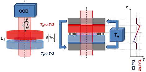
Figure 1: Scheme of the experimental cell: two sapphire windows are kept at different temperatures $T_{0}+\Delta T/2$ (the top, red one) and $T_{0}-\Delta T/2$ (the bottom, blue one) while the sample fluid (colored pattern) is contained by an O-ring (black circles) at a thickness $L$ precisely defined by three plastic spacers (gray rectangles).

Confinement is expected to cause deviations from Eq. (2) at very small wave numbers; to investigate this issue we perform experiments at wave vectors down to $q_{\text{min}}=8.9$ cm^-1. We apply a stabilizing temperature difference $\Delta T=20$ K (with an average temperature of $T_{0}=$298 K) to a horizontal layer of tetralin and n-dodecane at 50% weight fraction of different vertical thicknesses $L=$ 0.7, 1.3 and 5.0 mm and constant lateral extent $R=$ 13.0 mm. The sample thickness is varied by using different plastic spacers and sealing O-rings. Given the sample thermophysical properties properties the solutal Rayleigh numbers are: $Ra_{s}=-4\cdot 10^{4}$, $-2\cdot 10^{5}$ and $-1\cdot 10^{7}$, respectively. The thermal gradient cell is sketched in Fig. 1: two sapphire windows kept at fixed distance vertically contain the sample fluid and are thermally controlled by two Peltier elements with a central hole. The entire system allows a quasi-mono-chromatic parallel light beam pass through in the direction of the temperature gradient. More details of the thermal gradient cell can be found in previous literature croccolo_2012 ; croccolo_2013 .

The rapid imposition of a temperature difference by heating the fluid mixture from above results in a linear temperature profile across the sample in a thermal time $\tau_{T}=L^{2}/\kappa$, where $\kappa$ is the fluid thermal diffusivity. Due to the much smaller value of the mass diffusion coefficient, a nearly linear concentration profile is generated by means of the Soret effect soret_1879 ; book_degroot_1962 in a much larger solutal diffusion time $\tau_{s}=L^{2}/D$. Since the investigated mixture has a positive separation ratio, for negative $Ra_{s}$ both the temperature and the concentration profile result in a stabilizing density profile ryskin_2003 and the only variations are due to intrinsic fluctuations.

Shadowgraphy book_settles_2001 ; trainoff_2002 ; croccolo_2011 ; optical_setup allows recording images whose intensities $I(\mathbf{x},t)$ contain a mapping of the sample refractive index fluctuations, over space and time, averaged along the direction of the gradient, as illustrated in Fig. 2(a). These intensity patterns are generated at the sensor plane by the heterodyne superposition of the light scattered by the sample refractive index fluctuations and the much more intense transmitted beam (’local oscillator’). These images are 2D-space-Fourier transformed in silico, Fig. 2(c), to separate the contribution of light scattered at different wave vectors. This procedure provides results similar to conventional Light Scattering, but with a shadowgraph one can access smaller wave vectors, exactly were gravity and confinement effects are expected to strongly affect the c-NEFs.

Dynamic shadowgraphy is performed by the Differential Dynamic Algorithm croccolo_2007 ; croccolo_2012 ; croccolo_2006 ; cerbino_2008 , where one directly computes the so-called structure function:

$$C(q,\Delta t) =\langle\mid\Delta i_{m}(\mathbf{q},\Delta t)\mid^{2}\rangle_{t,\mid\mathbf{q}\mid=q}=$$

$$=\langle\mid i(\mathbf{q},t)-i(\mathbf{q},t+\Delta t)\mid^{2}\rangle_{t,\mid\mathbf{q}\mid=q},$$ (3)

with $i(\mathbf{q},t)=\mathcal{F}[I(\mathbf{x},t)/\langle I(\mathbf{x},t)\rangle_{\mathbf{x}}]$ the 2D-Fourier transform of a normalized image $I(\mathbf{x},t)$ and $\Delta t$ the time delay between the pair of analyzed images, as illustrated in Fig. 2(b-c). $C(q,\Delta t)$ is shown in Fig. 2(d-e). The structure function is related to the ISF via croccolo_2006 ; croccolo_2007 ; croccolo_2012 ; cerbino_2008 :

$$C(q,\Delta t)=2A\{T(q)S(q)\mid 1-f(q,\Delta t)\mid+B(q)\},$$ (4)

where $T(q)$ is the optical transfer function of the instrument (a complicated oscillating function for a shadowgraph, see trainoff_2002 ; croccolo_2011 ), $S(q)$ the static structure factor of c-NEFs, $A$ an intensity pre-factor, and $B(q)$ a background including all the phenomena with time-correlation functions decaying faster than the CCD frame rate, such as contributions due to shot noise and temperature fluctuations. The ISF $f(q,{t})$ can be evaluated via Eqs. (3)- (4). Results for three different wave vectors are shown in Fig. 2(f). Essentially for all the wave vectors accessible in the reported experiments the ISF can be fit by a single exponential function over the resolved part of the decay. For direct comparison with theory and simulations we extract effective decay times as the time needed to $f(q,{t})$ to decay to $1/e$.

Figure 3 reports experimental data for the three different $Ra_{s}$, not normalized in panel (a), and in dimensionless form in panel (b). For essentially all wave vectors smaller than $\tilde{q}_{s}^{\star}=\sqrt[4]{-Ra_{s}}$, the effective decay time departs from the theoretical description of Eq. (2) depicted as a dashed line. As the wave vector is decreased the decay time presents a minimum for a dimensionless wave vector $\tilde{q}_{b}\cong 5$ and for smaller wave vectors it recovers a diffusive decay $\tilde{\tau}\propto\tilde{q}^{-2}$ (except for $Ra_{s}=-1\cdot 10^{7}$, with no experimental points at low enough $\tilde{q}$).

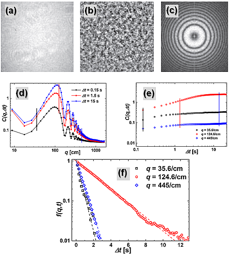
Figure 2: (a) Shadowgraph image $I(\mathbf{x},t)$; (b) difference of normalized images $\Delta i_{m}(\mathbf{x},\Delta t)$; (c) power spectrum of (b) $\mid\Delta i_{m}(\mathbf{q},\Delta t)\mid^{2}$; (d) structure function $C(q,\Delta t)$ for three different time delays, vertical lines stand for wave vectors used in (e); (e) structure function $C(q,\Delta t)$ for three different wave vectors, vertical lines stand for delay times used in (d); (f) ISFs for three different wave vectors $f(q,\Delta t)$: markers are for experimental data while lines depict theoretical results. All data are taken from the measurement at $Ra_{s}=-2\cdot 10^{5}$.

In order to interpret these experimental findings we use a Fluctuating Hydrodynamics (FHD) model dezarate_2006 that incorporates gravity and confinement. The dynamic structure factor $I(q,t)$ of the c-NEFs can be expressed as:

$$I(q,t)=S(q)f(q,t)=\sum\limits_{N=1}^{\infty}A_{N}(q)\exp\bigg{[}-\frac{t}{\tau_{N}(q)}\bigg{]},$$ (5)

see suppl for further details. The decay times in Eq. (5) are the inverse of the eigenvalues $\Gamma_{N}(q)=1/\tau_{N}(q)$ solving Eq. (43) in Ref. dezarate_2006 . The amplitudes $A_{N}$ are analytically related to $\Gamma_{N}$ and $q$. The power spectrum (static structure factor) of c-NEFs analyzed in dezarate_2006 is then $S(q)=\sum A_{N}(q)$. In general, the eigenvalues can only be computed numerically, however, in the limit $q\to 0$, a full analytical investigation is possible by means of power expansions in $q$, and a clear hierarchy of well-separated $\Gamma_{N}$ identified dezarate_2006 . In that limit, the first term in Eq. (5) dominates, and $f(q\to 0,t)$ becomes single-exponential in practice, with decay time due to confinement (c):

$$\tilde{\tau}(\tilde{q}\to 0)|_{c}=\frac{1}{\tilde{q}^{2}\Big{(}1-\dfrac{Ra_{s}}{Ra_{s,c}}\Big{)}}=\frac{1}{\tilde{q}^{2}\Big{(}1-\dfrac{Ra_{s}}{720}\Big{)}},$$ (6)

where $Ra_{s,c}=720$ is the critical solutal Rayleigh number at which the convective instability first appears ryskin_2003 . This asymptotic behaviour is shown in Fig. 3(b) by dotted lines. Hence, the theory predicts a crossover from Eq. (2) (not-including confinement) at large and intermediate $q$, to the confinement behaviour of Eq. (6) at small $q$, precisely the kind of behaviour experimentally shown in Fig. 3. We estimate the wave number $q_{b}$ corresponding to the minimum decay time by equating Eq. (2) and (6). This gives $\tilde{q}_{b}=\sqrt[4]{Ra_{s,c}}=\sqrt[4]{720}\cong 5.2$ independent of $Ra_{s}$, in further agreement with the observations in Fig. 3(b).

Previous work dezarate_2006 considered only small (in magnitude) negative solutal Rayleigh numbers. Here we investigate $Ra_{s}$ values for realistic liquid mixtures, and find different, much richer, $\Gamma_{N}(q)$ and $A_{N}(q)$ landscapes. In Fig. 4(a) the amplitudes $A_{N}(\tilde{q})$ of the first three eigenmodes are shown as a function of the dimensionless wave number $\tilde{q}$, for $Ra_{s}=-2\cdot 10^{5}$, while Fig. 4(b) shows the corresponding dimensionless decay times $\tilde{\tau}_{N}(\tilde{q})$ for the first two modes. Clearly in different wave number ranges different modes dominate. For very large ($\tilde{q}\gtrsim 50$) wave numbers, all decay times collapse and the ISF is approximately a single exponential dominated in amplitude by the first mode. For very small wave numbers ($\tilde{q}\lesssim 0.3$) the first mode dominates in amplitude and a single-exponential decay is again recovered. The second mode leads in amplitude in the central range $0.6\lesssim\tilde{q}\lesssim 30$, but having a smaller decay time means that both modes play a significant role and the ISF should show signatures of a double exponential decay. Indeed, data from theory and simulations show such signatures in the predicted wave vector range, however such signatures are not detectable in the experimental data given the limited wave vector range and the smaller signal to noise ratio. In Fig. 2(e) we report three examples of experimental ISFs for different wave vectors.

Also for the theory and regardless of the multiple exponential character, a single effective decay time $\tau_{\text{eff}}(q)$ is defined by $f(q,\tau_{\text{eff}})=1/e$. In Figs. 3 and 4(b) we show results for $\tau_{\text{eff}}(q)$, computed via Eq. (5) from the amplitudes and decay rates obtained theoretically. All the features seen in the experimental data points are well-reproduced by the theory. Noticeably the slowing-down observed for small wave numbers is clearly related to confinement, since this is the only ingredient added to the theory that gives Eq. (2).

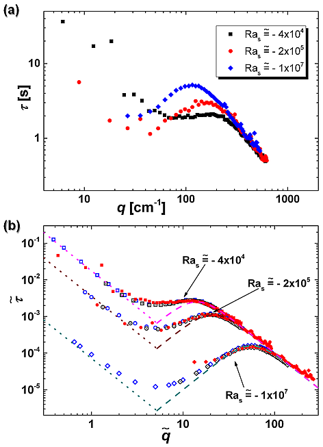
Figure 3: Effective decay times: (a) Log-log plot of the experimental decay times $\tau$ as a function of wave vector $q$ for different Rayleigh numbers. (b) Log-log plot of the dimensionless decay times $\tilde{\tau}$ as a function of dimensionless wave number $\tilde{q}$. Filled red markers are experimental data, open blue are for calculations based on the FHD model, and open-dotted black are from numerical simulations. Dashed lines depict the analytical solution provided by Eq. (2) for $\tilde{q}>\tilde{q_{b}}$, taking into account gravity and diffusion only; dotted lines are for the confinement limit of Eq. (6) for $\tilde{q}<\tilde{q_{b}}$.

The theory dezarate_2006 assumes that viscous dissipation dominates, and neglects the effect of fluid inertia; this is justified by the fact that in all liquids momentum diffusion is much faster than mass diffusion, i.e., the Schmidt number $\text{Sc}=\nu/D$ is very large. While neglecting inertial effects is a good approximation at most wavenumbers of interest, it is known that, depending on $Ra_{s}$, it fails at sufficiently small wavenumbers due to the appearance of inertial propagative modes takacs_2008 (closely related to gravity waves) driven by buoyancy. In order to confirm that the observed slowing down is due to confinement and not to inertia we have performed numerical simulations that account for inertial effects and confinement usabiaga_2012 ; delong_2014 , see suppl for details. Data points from a numerical simulation with fluid parameters matching the experimental ones are also shown in Fig. 3. An excellent agreement is visible for this dataset among experimental, theoretical and simulation results, confirming that inertia effects are not relevant in our experiments. We note, however, that for thicknesses $L\gtrsim 5$ mm the simulations do show oscillatory time correlation functions (propagative modes) at the smallest wavenumbers delong_2014 ; this range is not accessible in the experiments reported here.

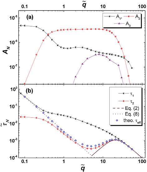
Figure 4: (a) Log-log plot of the amplitude of the first three eigenmodes $A_{N}$, for $N=1,2,3$, as a function of the dimensionless wave number $\tilde{q}$ for $Ra_{s}=-2\cdot 10^{5}$. (b) Log-log plot of the dimensionless decay times of the two first eigenvalues $\tilde{\tau}_{N}=\tau_{N}/\tau_{s}$, for $N=1,2$ as a function of the dimensionless wave number for the same $Ra_{s}$. Eqs. (2), (6) and the theoretical data points reported in Fig. 3 are also plotted for direct comparison.

We conclude that confinement has a moderate damping impact on the intensities of large-scale non-equilibrium concentration fluctuations, but, in the presence of gravity, it strongly affects their dynamics. Experiments, as well as theory and simulations, show that the slowing down is determined by the solutal Rayleigh number that, in this study, is controlled solely by the confinement distance $L$. Large-scale fluctuations are confined to evolve in an essentially quasi-two-dimensional manner by the boundaries, and we found them to behave diffusively but with a greatly enhanced diffusion coefficient.

This is in contrast to the case of diffusion in a microgravity environment where the coupling to velocity fluctuations greatly enhances the intensity of the c-NEFs but does not alter their Fickian diffusive dynamics vailati_2011 . In strongly confined systems, such as porous media, the buoyancy driven acceleration of the fluctuations is eliminated by confinement already at mesoscopic scales. In the absence of confinement, however, the gravitational acceleration is eventually suppressed by inertial effects leading to propagative modes; confinement is expected to also strongly affect the dynamics of these gravity waves, as we will explore in future work.

Although the main focus of this letter is on the dynamics and we leave for future publications a full discussion of the statics, we note that the minimum $\tilde{q}_{b}$ in $\tau_{\text{eff}}$ corresponds to a minimum in the intensity of fluctuations $S(q)$. This indicates that the results presented here may be thought of as a kind of de Gennes narrowing degennes_1959 . In analogy to diffusion in colloidal suspensions where a competition between interparticle interactions and hydrodynamic effects is present, here we have a competition between gravity and confinement.

Interestingly, we find that the dimensionless wave number identifying where confinement coexists with gravity is related to the critical solutal Rayleigh number $Ra_{s,c}=720$ where the convective instability first appears ryskin_2003 . This is a signature of the Onsager regression hypothesis stating that the dynamics of the fluctuations contains all of the signatures seen in the deterministic dynamics, which is known to be controlled by the Rayleigh number. Our work indicates that the study of the dynamics, rather than the intensity of non-equilibrium fluctuations, gives deep insights into the competition of physical processes such as diffusion, buoyancy, and confinement.

Correspondence and requests for materials should be addressed to F.C. (fabrizio.croccolo@univ-pau.fr)

References

- (1) T. R. Kirkpatrick, E. G. D. Cohen, and J. R. Dorfman, Phys. Rev. A 26, 995 (1982).
- (2) J. R. Dorfman, T. R. Kirkpatrick, and J. V. Sengers, Ann. Rev. Phys. Chem. 45, 213 (1994).
- (3) J. M. Ortiz de Zárate and J. V. Sengers, Hydrodynamic fluctuations in fluids and fluid mixtures (Elsevier, Amsterdam, 2006).
- (4) J. V. Sengers and J. M. H. L. Sengers, Annu. Rev. Phys. Chem. 37, 189 (1986).
- (5) A. Vailati and M. Giglio, Nature 390, 262 (1997).
- (6) A. Vailati and M. Giglio, Phys. Rev. E 58, 4361 (1998).
- (7) J. M. Ortiz de Zárate, J. A. Fornés and J. V. Sengers , Phys. Rev. E 74, 046305 (2006).
- (8) F. Croccolo, D. Brogioli, A. Vailati, M. Giglio and D. S. Cannell, Phys. Rev. E 76, 041112 (2007).
- (9) P. N. Segrè, R. Schmitz and J. V. Sengers , Physica A 195, 31 (1993).
- (10) P. N. Segrè, and J. V. Sengers , Physica A 198, 46 (1993).
- (11) F. Croccolo, D. Brogioli, A. Vailati, M. Giglio and D. S. Cannell, App. Opt. 45, 2166 (2006).
- (12) F. Croccolo, H. Bataller, and F. Scheffold, J. Chem. Phys. 137, 234202 (2012).
- (13) C. Giraudet, H. Bataller, and F. Croccolo, Eur. Phys. J. E, 37, 107 (2014).
- (14) F. Croccolo, H. Bataller, and F. Scheffold, Eur. Phys. J. E, 37, 105 (2014).
- (15) g cm-3, cm2s-1, cm2s-1, K-1, K-1, , from platten_2003 and references therein.
- (16) J. K. Platten, M. M. Bou-Ali, P. Costesèque, J. F. Dutrieux, W. Köhler, C. Leppla, S. Wiegand, and G. Wittko, Phil. Mag. 83, 1965 (2003).
- (17) F. Croccolo, F. Scheffold and A. Vailati, Phys. Rev. Lett. 111, 014502 (2013).
- (18) C. Soret, Arch. Sci. Phys. Nat. 3, 48 (1879).
- (19) S. R. de Groot and P. Mazur, Nonequilibrium thermodynamics (North-Holland, Amsterdam, 1962).
- (20) A. Ryskin, H. W. Müller, and H. Pleiner, Phys. Rev. E 67, 046302 (2003).
- (21) G. S. Settles, Schlieren and Shadowgraph Techniques (Springer, Berlin, 2001).
- (22) S. Trainoff, and D. S. Cannell, Phys. Fluids 14, 1340 (2002).
- (23) F. Croccolo, and D. Brogioli, App. Opt. 50, 3419–3427 (2011).
- (24) The probing beam is a plane parallel beam of quasi-monochromatic light as in previous setups croccolo_2012 ; croccolo_2013 . After the sample no collecting lens is used. A Charged Coupled Device sensor (IDS, UI-6280SE-M-GL) with a resolution of pixels of is placed at a distance of mm from the detector. Images are cropped to square resolution of pixels. In this arrangement the size of the image is dictated by the real size of the CCD sensor, which is 7.066 mm. This fixes the minimum wave vector to .
- (25) R. Cerbino, and V. Trappe, Phys. Rev. Lett. 100, 188102 (2008).
- (26) See Supplemental Material at [URL will be inserted by publisher] for further details on the theoretical calculations, the numerical simulations, and an empirical fit to the data.
- (27) C. J. Takacs, G. Nikolaenko and D. S. Cannell, Phys. Fluids 100, 234502 (2008).
- (28) F. Balboa Usabiaga, J. B. Bell, R. Delgado-Buscalioni, A. Donev, T. G. Fai, B. E. Griffith, and C. S. Peskin, SIAM J. Multiscale Model. Simul. 10, 1369 (2012).
- (29) S. Delong, Y. Sun, B.E. Griffith, E. Vanden-Eijnden and A. Donev, Phys. Rev. E, 90,, 063312 (2014).
- (30) A. Vailati, R. Cerbino, S. Mazzoni, C. J. Takacs, D. S. Cannell and M. Giglio, Nature Comm. 2, 290 (2011).
- (31) P. G. de Gennes, Physica A 25, 825 (1959).