Bijections for simple and double Hurwitz numbers

Abstract

We give a bijective proof of Hurwitz formula for the number of simple branched coverings of the sphere by itself. Our approach extends to double Hurwitz numbers and yields new properties for them. In particular we prove for double Hurwitz numbers a conjecture of Kazarian and Zvonkine, and we give an expression that in a sense interpolates between two celebrated polynomiality properties: polynomiality in chambers for double Hurwitz numbers, and a new analog for almost simple genus 0 Hurwitz numbers of the polynomiality up to normalization of simple Hurwitz numbers of genus $g$. Some probabilistic implications of our results for random branched coverings are briefly discussed in conclusion.

1 Introduction

Hurwitz branched covering counting problem consists in determining the number of inequivalent $d$-sheet branched coverings of the 2-sphere $\mathcal{S}_{0}$ by a connected genus $g$ closed surface $\mathcal{S}_{g}$, with prescribed ramification types over some fixed set of critical points, most of which are simple. In the last decade, the topic has attracted renewed interest following the work of Okounkov and Pandharipande [27] showing how Hurwitz numbers could be used to derive an alternative proof of Konsevitch theorem (Witten conjecture, see also [19]), and that of Ekedahl, Lando, Shapiro and Vainshtein [11], revealing a tight relation between Hurwitz numbers and intersection theory of the moduli spaces of curves now known as ELSV formula (see e.g. [10] and references therein).

Of particular interest are the double Hurwitz numbers $h_{g}(\mu,\nu)$, indexed by a non-negative integer $g$ and two partitions $\mu$ and $\nu$ of $d$: they count $d$-sheet branched coverings of $\mathcal{S}_{0}$ by $\mathcal{S}_{g}$ with $r+2$ fixed ramified points, all of which are simple, except for the last two which have ramification type $\mu$ and $\nu$ respectively (each covering $f$ is counted with a weight $1/{\mathrm{Aut}(f)}$ and $r=m+n-2+2g$, $m$ and $n$ being the respective number of parts of $\mu$ and $\nu$). A variety of approaches have been used to study these double Hurwitz numbers, or their specialization to the simple Hurwitz numbers $h_{g}(\mu)=h_{g}(\mu,1^{d})$: cut-and-join equations [13, 7], the ELSV formula [11, 15, 29], character theoretic or infinite wedge approaches leading to integrable hierachies [26, 14, 17, 25, 10], matrix integrals [4], the topological recursion [12] and indirect bijective enumeration [5].

In this article, we introduce new combinatorial structures, Hurwitz mobiles, and a non-trivial one-to-one correspondence between branched coverings and these objects. Hurwitz mobiles are tree-like structures that are in some cases much easier to enumerate than branched coverings or any of their known combinatorial avatars (ribbon graphs, constellations, factorizations into transpositions, or tropical diagrams…), and we use this fact to derive results of different types:

a.

A 5 page self-contained bijective proof of Hurwitz formula for genus 0 simple Hurwitz numbers (modulo standard results about trees).

b.

For any fixed partition $\nu$, an analog for genus 0 almost simple Hurwitz numbers $h_{0}(\mu,\nu 1^{d-|\nu|})$ of the polynomiality property of positive genus simple Hurwitz numbers $h_{g}(\mu,1^{d})$ (Corollary 7).

c.

A simple expression as a sum of explicit positive monoms indexed by trees for the polynomials giving double Hurwitz numbers in chambers (Corollary 4), and related results.

d.

A proof of a conjecture of Kazarian and Zvonkine about the dependency in $d$ of double Hurwitz numbers $h_{0}(\mu 1^{d-|\mu|},\nu 1^{d-|\nu|})$ when $\mu$ and $\nu$ are fixed, and new explicit formulas for these numbers with a remarkable positivity property (Theorem 3.2).

Our main correspondence directly extends to higher genus and we believe that a. could be adapted to give a common generalization of b. and the polynomiality properties of higher genus simple Hurwitz numbers, but we have not done this yet. Along with c. we can rederive the chamber structure of Hurwitz numbers (in particular the so-called resonances have a nice interpretation in our setting, as well as Shadrin, Shapiro, Vainstein’s recurrence relation for wall crossing formulas [29]) but we feel that this is not so interesting even from a combinatorial perspective because, as shown by Cavalieri et al [7], these results follow from the direct combinatorial interpretation of the cut and join equation which is more elementary than our approach. Regarding d., we prove that for any two fixed partitions $\mu$ and $\nu$, with $|\mu|\geq|\nu|$ (assumed for the moment without parts equal to one for simplicity), the double Hurwitz numbers $h_{0}(\mu 1^{d-|\mu|},\nu 1^{d-|\nu|})$ can be expanded after proper normalization as polynomials in $d$:

$$\frac{h_{0}(\mu 1^{d-|\mu|},\nu 1^{d-|\nu|})}{(m+n+2d-|\mu|-|\nu|-2)!}=\frac{d^{d+m+n-3}}{d!}\frac{(d)_{|\mu|}}{d^{|\mu|}}\frac{q_{\mu,\nu}(1/d)}{\mathrm{Aut}(\mu)\mathrm{Aut}(\nu)}$$ (1)

where $(d)_{k}=d(d-1)\cdots(d-k+1)$ and $q_{\mu,\nu}(z)$ is a polynomial of degree $|\nu|$, as conjectured by Kazarian and Zvonkine. Moreover, we give a combinatorial description of the coefficients of the polynomials $q_{\mu,\nu}(z)$ in Theorem 3.2, and we show their dependancy in the parts of $\mu$ and $\nu$. For instance, for any $\alpha\geq\beta\geq 2$, we prove

$$\frac{h_{0}(\alpha 1^{d-\alpha},\beta 1^{d-\beta})}{(2d-\alpha-\beta)!}=\frac{d^{d-1}}{d!}\frac{\alpha^{\alpha}}{\alpha!}\frac{\beta^{\beta}}{\beta!}\left(\frac{(d)_{\alpha+\beta}}{d^{\alpha+\beta}}+\frac{1}{d}\cdot\sum_{\ell=1}^{\beta}\frac{(d)_{\alpha+\beta-\ell}}{d^{\alpha+\beta-\ell}}\frac{(\alpha)_{\ell}}{\alpha^{\ell}}\frac{(\beta)_{\ell}}{\beta^{\ell}}(\alpha+\beta-\ell)\right).$$ (2)

The cases $\{\alpha,\beta\}\subset\{2,3\}$ of this formula were previously published in [31, 18] and an algorithm to compute the coefficients for fixed $\alpha$ and $\beta$ is given in [18] together with explicit formulas for larger values of $\alpha$ and $\beta$ but to the best of our knowledge the closed form above is new. In particular our formulas have the remarkable property that that they involve summation of positive contributions so that they are cancellation free (as opposed e.g to formulas in [31] or [25]).

Our polynomiality result for genus 0 almost-simple Hurwitz numbers is in fact a further generalization of the result above: for each partition $\nu$ we prove combinatorially that there exist polynomials $q_{\lambda,\kappa}^{\nu}$ in $m$ such that for all partitions $\mu=(\mu_{1},\ldots,\mu_{m})$ of an integer $d\geq|\nu|$,

$$\frac{h_{0}(\mu,\nu 1^{d-|\nu|})}{(m+n+d-|\nu|-2)!}=\frac{d^{d-2-|\nu|}}{\mathrm{Aut}(\mu)}\prod_{i=1}^{m}\frac{\mu_{i}^{\mu_{i}}}{\mu_{i}!}\sum_{\begin{subarray}{c}\lambda,\kappa\mid|\lambda|+|\kappa|<|\nu|\end{subarray}}q_{\lambda,\kappa}^{\nu}(m)\cdot\mathbf{m}_{\lambda;\kappa}(\mu_{1},\ldots,\mu_{m})$$ (3)

where $\mathbf{m}_{\lambda;\kappa}$ denote the monomial symmetric Laurent polynomial of shape $(\lambda;\kappa)$. In particular for $\nu=1$, the summation restricts to $\lambda=\kappa=\varepsilon$ the empty partition and $q^{1}_{\varepsilon,\varepsilon}=\mathbf{m}_{\varepsilon,\varepsilon}=1$ so that Formula (3) is Hurwitz formula. More generally, we derive the above structural result from an explicit expression of double Hurwitz numbers as a finite sum of positive contributions indexed by simple combinatorial structures. Again the existence of formulas in terms of symmetric functions in the parts had been observed for small values of $\nu$ by Kazarian [18]. Our main interpretation of Hurwitz numbers, Theorem 2.1, can be understood as a combinatorial interpolation between these various polynomiality results.

To obtain our main correspondence, we adapt to Hurwitz’ problem an approach that has been developed in the last 15 years in the combinatorial study of planar maps [28, 8, 3, 2, 1], and that has allowed in particular to show that properly rescaled large random planar maps admit a non trivial continuum limit, the Brownian map [21, 24]. In this context, two main strategies have emerged, based on the one hand on minimal orientations and so-called blossoming trees (see [1]), and on the other hand on geodesic labeling and so-called mobiles (see [8, 6, 3, 2]). In [9] we have shown that the first approach could be extended to derive a first bijective proof of Hurwitz’ explicit formula for genus 0 simple Hurwitz numbers. However this first approach does not extend to higher genus and becomes more intricate in the case of double Hurwitz numbers. The present paper builds on the second strategy and in particular on Bouttier, Di Francesco, and Guitter’s bijection between bipartite maps and mobiles [6]. Refining and adapting this approach yields a different bijective proof of Hurwitz formula, that extends nicely to double Hurwitz numbers. As discussed in the conclusion we hope that theses results could lead, as in the case of planar maps, to a better understanding of the combinatorial geometry of branched coverings, and in particular to a proof that a properly chosen model of rescaled random branched coverings converges to the Brownian map.

2 Statement of the main bijection

2.1 Hurwitz numbers and galaxies

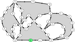
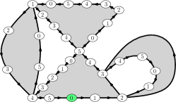
Figure 1: Two marked galaxies with respective type $(31^{5},2^{4})$ and $(321,2^{2}1^{2})$. The right one is a Hurwitz galaxy.

Our starting point is a standard representation of branched coverings of the sphere in terms of embedded graphs (aka ribbon graphs) which, following the combinatorial literature, we call maps.

A map of genus $g$ is a cellular embedding of a graph in $\mathcal{S}_{g}$, the compact oriented surface of genus $g$, that partitions it into 0-cells (vertices), 1-cells (edges) and 2-cells (faces), and considered up to orientation preserving homeomorphisms of $\mathcal{S}_{g}$. A map is bicolored if its faces are colored in black or white so that adjacent faces have different colors. The canonical orientation of a bicolored map is the orientation of edges such that each edge has a black face on its left. For any $r\geq 2$, a $r$-galaxy of genus $g$ is a map of genus $g$ which is bicolored and such that the length of any oriented cycle is a multiple of $r$. A galaxy is marked if it has a distinguished vertex. There is a unique way to color the vertices of a marked galaxy with colors $\{0,\ldots,r-1\}$ so that the marked vertex $x_{0}$ has color 0 and each edge points from a vertex of color $i$ to a vertex of color $(i+1\mod r)$: the color of any vertex $x$ is given by the reminder modulo $r$ of the length of any oriented path from $x_{0}$ to $x$. By construction the number of edges whose origin has color $i$ is the same for all $i$, and this common number is the size of the galaxy. Two examples of marked galaxies are given in Figure 1.

From now on in this section, let $r\geq 2$, $g\geq 0$ and $d\geq 1$ be fixed integers, and let a Hurwitz galaxy be a marked $(r+1)$-galaxy of size $d$ and genus $g$ whose vertices all have half-degree one apart from $r$ vertices with half-degree two, one for each color $c=1,\ldots,r$ (because of the bicoloration of faces, vertices of galaxies have even degrees and their half-degree represent their number of incidences with black faces). Since a marked $(r+1)$-galaxy of genus $g$ and size $d$ has $d$ edges originating from vertices of color $i$ for each $c=0,\ldots,r$, it is a Hurwitz galaxy if and only if it has exactly $d-1$ vertices of each color $c$, $c=1,\ldots,r$, and $d$ vertices of color $0$ (including the marked vertex). The type of a galaxy $G$ is the pair of partition $\mu=1^{m_{1}}\ldots d^{m_{d}}$, $\nu=1^{n_{1}}\ldots d^{n_{d}}$ of $d$ where $m_{i}$ is the number of white faces of degree $(r+1)i$ in $G$ and $n_{i}$ is the number of black faces of degree $(r+1)i$ in $G$. For any pair of partitions $\mu$ and $\nu$ with $|\mu|=|\nu|=d$ and $\ell(\mu)=m$, $\ell(\nu)=n$ and $r=m+\ell-2+2g$, let $\mathcal{H}_{g}(\mu,\nu)$ denote the set of Hurwitz galaxies of type $(\mu,\nu)$.

Proposition 1 (Folklore, see e.g. [20, Chapter 1] or [16])

Let $h^{\bullet}_{g}(\mu,\nu)$ denote the number of Hurwitz galaxies of type $(\mu,\nu)$ and genus $g$. Then:

• The standard Hurwitz numbers, $h_{g}(\mu,\nu)=\frac{1}{d}h^{\bullet}_{g}(\mu,\nu)$, count equivalence classes of branched coverings $f$ of the sphere by $\mathcal{S}_{g}$ with simple ramifications over $r$ fixed points $a_{1},\ldots,a_{r}$ and ramification of branching type $\mu$ and $\nu$ over two fixed points $w$ and $b$, with a weight $\frac{1}{\mathrm{Aut}(f)}$ (two branched coverings $f$ and $f^{\prime}$ are equivalent if there is an homeomorphism $h:\mathcal{S}_{g}\to\mathcal{S}_{g}$ that maps one onto the other, that is, $f^{\prime}=f\circ h$).

• The labelled Hurwitz numbers, $h^{\ell}_{g}(\mu,\nu)=(d-1)!h^{\bullet}_{g}(\mu,\nu)$, count transitive factorizations $(\tau_{1},\ldots,\tau_{r},\sigma,\rho)$ of the identity permutation of $\mathfrak{S}_{d}$, where $r=m+n-2+2g$, the permutations $\sigma$ and $\rho$ have cyclic type $\mu$ and $\nu$ respectively, and the $\tau_{i}$ are transpositions.

Some authors prefer to work with $h_{g}(\mu,\nu)$, others with $h_{g}^{\ell}(\mu,\nu)$. Finally, following [31], let the normalized Hurwitz numbers be defined as follows: let $\mathbf{x}=(x_{1},\ldots,x_{m})$ and $\mathbf{y}=(y_{1},\ldots,y_{n})$ be compositions of respective type $\mu$ and $\nu$ (that is, $\mathbf{x}$ is a permutation of the parts of $\mu$), and

$$\bar{h}_{g}(\mathbf{x},\mathbf{y})=\frac{\mathrm{Aut}(\mu)\mathrm{Aut}(\nu)}{(m+n-2+2g)!}h^{\bullet}_{g}(\mu,\nu),$$

where $\mathrm{Aut}(\mu)=m_{1}!\cdots m_{d}!$ if $m=1^{m_{1}}2^{m_{2}}\ldots d^{m_{d}}$. Then $(m+n-2+2g)!\bar{h}_{g}(\mathbf{x},\mathbf{y})$ is the number of branched coverings as above with the preimages of $w$ labeled by the integers $1,\ldots,m$ and the preimages of $b$ labeled by the integers $1,\ldots,n$, in such a way that the $i$th preimage of $w$ has order $x_{i}$ and the $i$th preimage of $b$ has order $y_{i}$. The reason for all these trivial variants is that explicit formulas are best stated with $h_{g}^{\bullet}(\mu,\nu)$ or $h_{g}(\mu,\nu)$, while the piecewise polynomiality properties hold for $\bar{h}_{g}(\mathbf{x},\mathbf{y})$.

Detailed definitions of branched coverings, maps on surfaces and related concepts (monodromy, factorizations of permutations) can be found in [20, Chapter 1]. As explained there, galaxies are obtained by taking the preimage of a well chosen curve on the sphere, and more generally, this process yields bijections between branched covers and various families of maps: these differents bijections are in a sense trivial, they just amount to different representations of the same underlying branched covering. Galaxies explicitely appear in [16] where they are refered to under the generic term ribbon graphs. We use the term galaxy because these maps generalize the constellations of [20].

2.2 Distances in galaxies

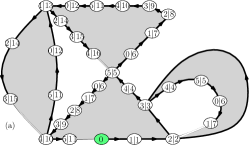
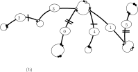
Figure 2: (a) Distances and non-geodesic edges: each vertex is labeled (color $|$ distance); non-geodesic edges are highlighted with lighter stroke. (b) An edge-labeled free Hurwitz mobile of type $(3\,2\,1,2^{2}1^{2})$, i.e. with one white 3-gon, and one white 2-gon, and one white 1-gon, and two black 2-gons, and two black 1-gons. (The weight of each edge is indicated by the number of transversal bars.)

Consider a Hurwitz galaxy endowed with its canonical orientation, and let $x_{0}$ denote the marked vertex. The underlying non-oriented map is connected by definition, and each oriented edge belongs to a cycle (e.g. turning around its incident black face), therefore any vertex can be reached by an oriented path from $x_{0}$. The distance labeling of a vertex $x$ is the number $\delta(x)$ of edges in a shortest oriented path from $x_{0}$ to $x$ (see Figure 2(a)). This distance labeling on a marked galaxy satisfies several immediate properties:

1. The color and distance label of a vertex $x$ are related by $c(x)=(\delta(x)\mod r+1)$.

2. For any (canonically oriented) edge $e=x\to y$, $\delta(y)\equiv\delta(x)+1\mod r+1$, and $\delta(y)\leq\delta(x)+1$.

We can thus define the weight of an edge $e=x\to y$ as the non-negative integer quantity $w(e)=(\delta(x)+1-\delta(y))/(r+1)$. An edge $e=x\to y$ with weight 0 is called geodesic. In other terms any edge $e=x\to y$ satisfies $\delta(y)=\delta(x)+1-(r+1)w(e)$, and it is geodesic iff $w(e)=0$. Since the sum of the variations of labels around each face must be zero, we have the following property:

1. The sum of the weight of the edges incident to any face with degree $(r+1)i$ is $i$.

2.3 Free Hurwitz mobiles

A Hurwitz mobile of type $(\mu,\nu)$ and excess $2g$ is a connected partially oriented graph made of

• $d$ white nodes forming $m_{i}$ disjoint oriented simple cycles of length $i$, for $i=1,\ldots,d$; each such cycle we refer to as a white polygon,

• $d$ black nodes forming $n_{i}$ disjoint oriented simple cycles of length $i$, for $i=1,\ldots,d$; each such cycle we refer to as a black polygon,

• $r+1=m+n-1+2g$ non-oriented edges with non-negative weights such that

  • each zero weight edge has both endpoints on white polygons

  • each positive weight edge is incident to a black and a white polygon

  • the sum of the weights of the edges incident to each $i$-gon is $i$.

A Hurwitz mobile is edge-labeled if its $m+n-1+2g$ weighted edges have distinct labels taken in the set $\{0,\ldots,m+n-2+2g\}$. Let us denote by $\mathcal{M}_{g}(\mu,\nu)$ the set of edge-labeled Hurwitz mobiles of type $(\mu,\nu)$ and excess $2g$. Hurwitz mobiles with excess 0 are called free Hurwitz mobiles. An example is given in Figure 2(b). Since a free Hurwitz mobile is a connected graph with $m+n-1$ weighted edges connecting $m+n$ polygons, these edges and polygons form a tree-like structure.

  

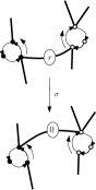
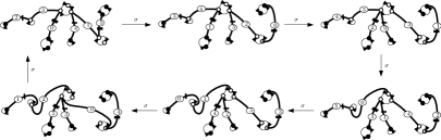
Figure 3: The shift operation. The shift equivalence class of the mobile of Figure 2.

Given an edge-labeled Hurwitz mobile $M$, its shift $\sigma(M)$ is the Hurwitz mobile obtained by translating the two endpoints of the edge with label $r$ along the polygon arc they are respectively incident to, and then incrementing all edge labels, modulo $r+1$ (so that the edge with label $r$ gets label $0$). Two edge-labeled Hurwitz mobiles are shift-equivalent if one can be obtained from the other by a sequence of shifts. As illustrated by Figure 3, $\sigma^{r+1}(M)=M$, and we shall later prove more precisely (Proposition 6) that each shift-equivalence class contains exactly $r+1$ distinct Hurwitz mobiles, so that the number of equivalence classes of edge-labeled Hurwitz mobiles of type $(\mu,\nu)$ and exces $2g$ is $\frac{1}{r+1}|\mathcal{M}_{g}(\mu,\nu)|$.

Finally, a Hurwitz mobile is face-labeled if its white polygons have distinct labels taken in $\{1,\ldots,m\}$ and its black polygons have distinct labels taken in $\{1,\ldots,n\}$. The type of a face-labeled Hurwitz mobile is the pair $(\mathbf{x},\mathbf{y})$ of compositions $\mathbf{x}=(x_{1},\ldots,x_{m})$, $\mathbf{y}=(y_{1},\ldots,y_{n})$ such that the $i$th white polygon is a $x_{i}$-gon and the $i$th black polygon is a $y_{i}$-gon. Let us denote $\bar{{\mathcal{M}}}_{g}(\mathbf{x},\mathbf{y})$ the set of face-labeled Hurwitz mobiles with type $(\mathbf{x},\mathbf{y})$ and excess $2g$. Then by an immediate double counting argument, edge-labeled and face-labeled Hurwitz mobile numbers are simply related:

$${\mathrm{Aut}(\mu)}\,{\mathrm{Aut}(\nu)}|{\mathcal{M}}_{g}(\mu,\nu)|=(m+n-1+2g)!|\bar{{\mathcal{M}}}_{g}(\mathbf{x},\mathbf{y})|.$$

2.4 The main bijection $\Phi$

Given a Hurwitz galaxy $G$ endowed with its distance labeling, we now construct a (partially oriented) graph $\Phi(G)$ made of oriented polygons connected by non-oriented edges according to the following local rules:

• (i) Polygons. Place in each face of degree $i(r+1)$ of $G$ an oriented $i$-gon (clockwise in white faces, ccw in black ones): the nodes and arcs of these polygons will be the nodes and arcs of $\Phi(G)$.

To make easier the description of the next step in the construction, let us moreover join with dashed lines the $i$ nodes in each face of degree $i(r+1)$ to the middles of the $i$ edges with color $r\to 0$ on its boundary: this divides each face $F$ of degree $(r+1)i$ of $G$ in $i+1$ sub-regions: the interior of the polygon, and $i$ sub-regions each containing on its boundary a subpath with color $0\to 1\to\ldots\to r$ of the boundary of $F$.

• (ii) Positive weight edges. For each non-geodesic edge $e=u\to v$ from a vertex $u$ with distance label $\delta(u)=i$ to a vertex $v$ with distance label $\delta(v)=i+1-\omega\cdot(r+1)$ ($\omega\geq 1$), let $F_{\circ}$ and $F_{\bullet}$ be the white and black faces incident to $e$, and let $x$ (resp. $y$) denote the origin of the unique arc of $\Phi(G)$ incident to the same sub-region of $F_{\circ}$ (resp. $F_{\bullet}$) as $v$. As illustrated in Figure 4(a), create in $\Phi(G)$ an edge with label $c(v)$ and weight $\omega$ between $x$ and $y$.

• (iii) Zero weight edges. For each vertex $v$ of $G$ with distance label $\delta(v)=j$ and color $c(v)$ that has two incoming geodesic edges, let $F_{\circ}$ and $F_{\circ}^{\prime}$ denote the two incident white faces, and let $y$ (resp. $y^{\prime}$) denote the origin of the unique arc of $\Phi(G)$ incident to the same sub-region of $F_{\circ}$ (resp. $F_{\circ}^{\prime}$) as $v$. As illustrated in Figure 4(b), create in $\Phi(G)$ an edge with label $c(v)$ and weight zero between $y$ and $y^{\prime}$. (For later purpose one should imagine that $v$ is split in two by the drawing of this new edge, as suggested by the figure.)

The application of the main bijection to the exemple of Figure 2(a) is given in Figure 4(c).

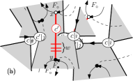
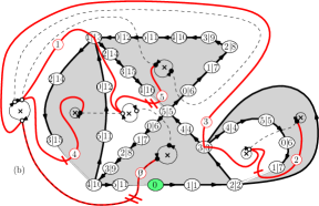
Figure 4: Construction rules: (a) for a non-geodesic edge (for conciseness $c=c(u)$, $c^{\prime}=c(v)$), and (b) for a vertex with 2 incoming geodesic edges ($c^{\prime}=c(v)$, $c\equiv c^{\prime}-1$). (c) The construction applied to the galaxy $G$ of Fig. 2(a). The resulting graph is the Hurwitz mobile of Fig. 2(b)

Theorem 2.1

The image $\Phi(G)$ of a Hurwitz galaxy $G$ with genus $g$ is an edge-labeled Hurwitz mobile with genus $g$, and the application $\Phi$ is injective. Moreover, in the case $g=0$, it is a 1-to-1 correspondence between Hurwitz galaxies of genus $0$ and shift-equivalence classes of edge-labeled free Hurwitz mobiles with the same type.

Corollary 1

Genus zero Hurwitz numbers count shift-equivalence classes of edge-labeled free Hurwitz mobiles,

$$h^{\bullet}_{0}(\mu,\nu)=\frac{1}{m+n-1}\;|{\mathcal{M}}_{0}(\mu,\nu)|,$$

and, consequently, normalized genus zero Hurwitz numbers count face-labeled free Hurwitz mobiles,

$$\bar{h}_{0}(\mathbf{x,y})=|\bar{{\mathcal{M}}}_{0}(\mathbf{x},\mathbf{y})|.$$

The application $\Phi$ is in fact a 1-to-1 correspondence between Hurwitz galaxies of genus $g$ and shift-equivalence classes of some particular Hurwitz mobiles of excess $2g$ called coherent Hurwitz mobiles of genus $g$. However we postpone the statement of the corresponding Theorem 4.1 to Section 4 where we prove that $\Phi$ is bijective, because the definition of these higher genus coherent Hurwitz mobiles has a non-trivial twist which makes enumerative consequences harder to derive.

We would like to insist on the fact that this result is not just a reformulation of Cavalieri et al combinatorial interpretation of the cut-and-join equation [7]. Free Hurwitz mobiles are significantly simpler to count than branched coverings or the associated tropicalized diagram, even in the planar case. To support this assertion, we observe that the representation of Cavalieri et al does not allow, as far as we know, to derive directly the original Hurwitz formula for $h_{0}(\mu,1^{d})$. Instead, as shown in Section 3.1, Theorem 2.1 easily results in a bijective proof of this formula.

3 Enumerative consequences

3.1 A bijective proof of Hurwitz’ formula

In the case $\nu=1^{d}$ of simple Hurwitz numbers, free Hurwitz mobiles are easy to count:

Proposition 2 (Hurwitz formula)

The number of Hurwitz mobiles in $\mathcal{M}_{0}(\mu,1^{d})$ is

$$|\mathcal{M}_{0}(\mu,1^{d})|={d+m-1\choose m-1}\cdot\frac{1}{m}{m\choose m_{1},\ldots,m_{d}}d^{m-2}\cdot d!\prod_{i\geq 1}\left(\frac{i^{i}}{i!}\right)^{m_{i}}$$

and as a consequence

$$h^{\bullet}_{0}(\mu,1^{d})=d^{m-2}\cdot(d+m-2)!\cdot\prod_{i\geq 1}\frac{1}{m_{i}!}\left(\frac{i^{i}}{i!}\right)^{m_{i}}.$$

Proof

By definition, when $\nu=1^{d}$, all black polygons are 1-gons, each incident to only one positive edge. As a consequence all positive edges have weight 1, and these positive edges are pending edges attached to white polygons. By definition again, each white $i$-gons is incident to $i$ such pending edges. Finally the white polygons and zero weight edges form a Cayley cactus, that is a tree-like structure consisting of $m$ polygons connected by $(m-1)$ labeled edges. Let us conversely consider the number of ways to construct Hurwitz mobiles by first building a Cayley cactus with edge labels forming a $(m-1)$-element subset $I$ of $\{0,\ldots,d+m-1\}$, and then adding zero weight edges and black 1-gons.

Let $I$ be one of the ${d+m-1\choose m-1}$ subsets of $m-1$ elements of $\{0,\ldots,d+m-1\}$. The number of Cayley cacti with $m_{i}$ white $i$-gons ($i=1,\ldots,d$) and $m-1$ labeled edges having distinct labels in $I$ is well known to be

$$\frac{1}{m}{m\choose m_{1},\ldots,m_{d}}d^{m-2}.$$

(This is a simple extension of Cayley formula, which corresponds to the case $\mu=1^{d}$. A proof follows from Lagrange inversion formula applied to the exponential generating function of these cacti or by a direct Prüfer encoding, see e.g. [30, Chap. 5]). The number of ways to distribute the remaining $d$ labels to the polygons of a Cayley cactus so that each $i$-gon gets a subset of $i$ labels is

$${d\choose\mu}=\frac{d!}{\prod_{i\geq 1}{(i!)^{m_{i}}}}$$

Each free Hurwitz mobile is then uniquely obtained from such a cactus by assigning each of the $i$ extra labels of each $i$-gon to an edge carrying a black 1-gon attached to one of the $i$ nodes of the $i$-gon: the total numbers of way to do this assignment is $\prod_{i\geq 1}(i^{i})^{m_{i}}$. The number of free Hurwitz mobiles of type $(\mu,1^{d})$ is thus

$${d+m-1\choose m-1}\cdot\frac{1}{m}{m\choose m_{1},\ldots,m_{d}}d^{m-2}\cdot d!\prod_{i\geq 1}\left(\frac{i^{i}}{i!}\right)^{m_{i}}$$

and Hurwitz formula follows. $\Box$

3.2 A shape formula for double Hurwitz numbers

From now on in this section, let $\mathbf{x}=(x_{1},\ldots,x_{m})$ and $\mathbf{y}=(y_{1},\ldots,y_{n})$ be two compositions of $d$ and let $r=m+n-2$. In order to obtain formulas for $\bar{h}_{0}(\mathbf{x},\mathbf{y})$ we classify face-labeled Hurwitz mobiles according to their weighted skeleton, that is, the bipartite graph with weighted edges obtained upon contracting each polygon into a vertex and removing zero weight edges, and even more coarsly according to their bare skeleton, the unweighted bipartited graph obtained from the weighted skeleton by forgetting the edge weights. Let us define $\mathcal{S}_{m,n}$ as the set of bare shapes, that is bipartite graphs on the vertex set $\{1,\ldots,m\}\cup\{1,\ldots,n\}$ without cycles or isolated vertices. The bare skeleton of a face-labeled Hurwitz mobile of $\bar{\mathcal{M}}_{0}(\mathbf{x},\mathbf{y})$ is clearly an element of $\mathcal{S}_{m,n}$, but to describe the elements of $\mathcal{S}_{m,n}$ that can be bare skeletons of Hurwitz mobiles in $\bar{\mathcal{M}}_{0}(\textbf{x},\textbf{y})$ we need some notations.

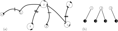
Figure 5: (a) A face-labeled Hurwitz mobile with $\mathbf{x}=(2,3,1)$ and $\mathbf{y}=(2,1,2,1)$. (b) Its bare skeleton. The edge weight vector is $\ell=(2,1,2,1)$ with edges enumerated from left to right. The degree and excess vectors are $d^{\circ}=(1,2,1)$, $\varepsilon^{\circ}=(1,1,0)$, $d^{\bullet}=(1,1,1,1)$ and $\varepsilon^{\bullet}=(1,0,1,0)$.

Given a bare shape $s$, let $|s|$ denote its number of edges, and $c(s)=m+n-|s|$ its number of connected components, and $d^{\circ}_{i}(s)$ (resp. $d^{\bullet}_{i}(s)$) the degree of the $i$th white (resp. black) vertex of $s$. In view of the vertex labels, bare shapes have no nontrivial automorphisms, thus we can assume that their edges are canonically labeled from 1 to $|s|$. Let us denote by $s^{\circ}_{j}$ and $s^{\bullet}_{j}$ the white and black rooted subtrees around the $j$th edge, and given a subgraph $s^{\prime}$ of a bare shape $s$, let $W(s^{\prime})$ and $B(s^{\prime})$ respectively denote the sets of indices of white and black vertices that belong to $s^{\prime}$. With these notations, for any $s\in\mathcal{S}_{m,n}$, let $C(s)$ be the region of $\mathbb{R}^{m+n}$ defined by the inequalities

$$\sum_{i\in W(s^{\circ}_{j})}x_{i}>\sum_{i\in B(s^{\circ}_{j})}y_{i}$$

for each edge $j$ of $s$, $j=1,\ldots,|s|$, and the equalities

$$\sum_{i\in W(s_{j})}x_{i}=\sum_{i\in B(s_{j})}y_{i}$$

for each connected component $s_{j}$ of $s$, $j=1,\ldots,c(s)$.

Theorem 3.1

The normalized Hurwitz number of type $(\mathbf{x},\mathbf{y})$ with $|\mathbf{x}|=|\mathbf{y}|=d$ is

$$\bar{h}_{0}(\mathbf{x},\mathbf{y})=\sum_{s\in\mathcal{S}_{m,n}}\left(d^{c(s)-2}\prod_{i=1}^{m}x_{i}^{d^{\circ}_{i}(s)-1}y_{i}^{d^{\bullet}_{i}(s)-1}\prod_{j=1}^{c(s)}\left(\sum_{i\in W(s_{j})}x_{i}\right)\cdot\chi_{(\mathbf{x},\mathbf{y})\in C(s)}\right)$$

where $\chi$ is the characteristic function: $\chi_{P}=1$ if $P$ is true, $0$ otherwise.

In particular for fixed $m$ and $n$, the number of regions $C(s)$ to be considered is finite and $\bar{h}_{0}(\mathbf{x},\mathbf{y})$ is a piecewise polynomial.

In order to prove the theorem, let us define a weighted shape as a pair $(s,\ell)$ where $s$ is a bare shape and $\ell=(\ell_{1},\ldots,\ell_{|s|})$ is a $|s|$-uple of positive integers, where $\ell_{j}$ is to be interpreted as the weight of the $j$th edge of $s$. Given a weighted shape $(s,\ell)$, let us denote by $x_{i}(s,\ell)$ (resp. $y_{i}(s,\ell)$) the sum of the weight of edges incident to the $i$th vertex of $s$, and by $\varepsilon^{\circ}_{i}(s,\ell)$ (resp. $\varepsilon^{\bullet}_{i}(s,\ell)$) the weight excess at $i$: $x_{i}(s,\ell)=d^{\circ}_{i}(s)+\varepsilon^{\circ}_{i}(s,\ell)$ (resp. $y_{i}(s,\ell)=d^{\bullet}_{i}(s)+\varepsilon^{\bullet}_{i}(s,\ell)$). The type of the weighted shape $(s,\ell)$ is the pair of compositions $(\mathbf{x}(s,\ell),\mathbf{y}(s,\ell))$ whose parts are the $x_{i}(s,\ell)$ and the $y_{i}(s,\ell)$.

Observe that in the above definition the $x_{i}=x_{i}(s,\ell)$ are actually linear combinations of the $\ell_{i}$: more precisely, if $E^{\circ}_{i}(s)$ denote the set of the edges incident to the $i$th white vertex in $s$, then $x_{i}=\sum_{j\in E^{\circ}_{i}(s)}\ell_{j}$, and similarly for the $i$th black vertex, $y_{i}=\sum_{j\in E^{\bullet}_{i}(s)}\ell_{j}$. Conversely, for any weighted shape $(s,\ell)$ of type $(\mathbf{x},\mathbf{y})$, the $\ell_{j}$ can be recovered from $s$ and $(\mathbf{x},\mathbf{y})$: let us denote by $s^{\circ}_{j}$ and $s^{\bullet}_{j}$ the white and black rooted subtrees around the $j$th edge: then $\ell_{j}=\ell_{s,j}(\mathbf{x},\mathbf{y})=\sum_{i\in W(s^{\circ}_{j})}x_{i}-\sum_{i\in B(s^{\circ}_{j})}y_{i}$. Similarly we also have the redundent equations $\ell_{j}=\ell_{s,j}(\mathbf{x},\mathbf{y})=\sum_{i\in B(s^{\bullet}_{j})}y_{i}-\sum_{i\in W(s^{\bullet}_{j})}x_{i}$.

This discussion implies that if a Hurwitz mobile $M$ of $\mathcal{M}_{0}(\mathbf{x},\mathbf{y})$ has bare skeleton $s$, then $(\textbf{x},\textbf{y})\in C(s)$: Indeed the weighted skeleton of $M$ has positive weights on every edge by construction. Moreover the sum of the weights of edges inside each component is by definition equals to the sum of the $x_{i}$s and to the sum of the $y_{i}$s in this component.

The theorem then follows from the converse analysis of the number of face-labeled free Hurwitz mobiles having a given weighted skeleton $(s,\ell)$.

Lemma 1

The number of free face-labeled Hurwitz mobiles with weighted skeleton $(s,\ell)$ and type $(\mathbf{x},\mathbf{y})$ with $|\mathbf{x}|=|\mathbf{y}|=d$, edges and $c(s)=m+n-|s|$ components is

$$\left\{\begin{array}[]{ll}R_{s}(\mathbf{x},\mathbf{y})=\displaystyle d^{c(s)-2}\left(\prod_{i=1}^{m}x_{i}^{d^{\circ}_{i}(s)-1}\right)\left(\prod_{i=1}^{n}y_{i}^{d^{\bullet}_{i}(s)-1}\right)\prod_{j=1}^{c(s)}\left(\sum_{i\in W(s_{j})}x_{i}\right)&\textrm{ if $(\mathbf{x},\mathbf{y})\in C(s)$,}\\ 0&\textrm{ otherwise}\end{array}\right.$$

where $s_{j}$ denote the $j$th component of $s$ and $W(s_{j})$ its set of white vertices.

Proof

Let $s$ be a bare shape with $q=c(s)$ connected components, and let $(\mathbf{x},\mathbf{y})\in C(s)$. We construct the corresponding free face-labeled Hurwitz mobiles in three steps:

1. To obtain a free Hurwitz mobile with skeleton $s$, the $i$th white vertex of $s$ must first be replaced by a $x_{i}$-gone, and each incident edge must be attached to one of $x_{i}$ nodes of this polygon. The same apply to black vertices. There are

   $$\left(\prod_{i=1}^{m}x_{i}^{d^{\circ}_{i}-1}\right)\left(\prod_{i=1}^{n}y_{i}^{d^{\bullet}_{i}-1}\right)$$

   non-equivalent ways to perform these operations.

2. Each forest of bipartite cacti obtained at the previous step has $q$ components $s_{1},\ldots,s_{q}$. Let $W(s_{1})\cup B(s_{1}),\ldots,W(s_{q})\cup B(s_{q})$ denote the white and black node sets of these components. By construction, the $j$th component has $d_{j}=\sum_{i\in W(s_{j})}x_{i}$ white nodes. In each component, mark one of these $d_{j}$ white nodes: there are

   $$\prod_{j=1}^{c(s)}d_{j}=\prod_{j=1}^{c(s)}\left(\sum_{i\in W(s_{j})}x_{i}\right)$$

   ways to do that.

3. In order to form a free Hurwitz mobile from such a forest we need to connect the $q$ connected components by $q-1$ edges of weight zero. Upon considering the $j$th connected component as a unique marked polygon with $d_{j}$ white nodes, the problem reduces to the standard cactus construction: The number of ways to form a cactus by adding $q-1$ edges to a set of $q$ marked polygons such that the $j$th polygon has $d_{j}$ nodes is $(\sum_{j=1}^{q}d_{j})^{q-2}$ (according to the extended Cayley formula for cacti [30, Chapter 5]). In our case $\sum_{j=1}^{q}d_{j}=d$ so that the number of ways to construct a Hurwitz cactus from a forest as above is just $d^{q-2}$. $\Box$

Consider for instance the case $m=n=2$: the possible shapes are given in Figure 6, together with their contribution and their associated region. Observe that Theorem 3.1 is slightly more powerful than the previous piecewise polynomiality theorems in the literature (see [7]): in particular it immediately implies Hurwitz formula, which as far as we understand, does not easily follow from the latter.

Corollary 2 (Hurwitz’s formula)

Let $s$ be a shape contributing to Hurwitz formula, i.e. such that $(\mathbf{x},1^{d})\in C(s)$. In view of the condition $y_{i}=1$ for all $i$, all black vertices in $s$ are leaves, and $s$ is a collection of stars, that is, $c(s)=m$, $d^{\bullet}_{i}(s)=1$ and $d^{\circ}_{i}(s)=x_{i}$. The number of such star forests is $d!\;\prod_{i=1}^{m}\frac{1}{x_{i}!}$ and each contributes to a factor $d^{m-2}\prod_{i=1}^{m}x_{i}^{x_{i}}$ so that

$$\bar{h}_{0}(\mathbf{x},1^{d})=d!\;d^{m-2}\;\prod_{i=1}^{m}\frac{x_{i}^{x_{i}}}{x_{i}!}.$$

Corollary 3

Let $s$ be a shape contributing to $\bar{h}_{0}(\mathbf{x},d)$. In view of the condition $y_{1}=d$, $s$ is the unique (star) tree with one black vertex, that is, $c(s)=1$, $d^{\bullet}_{1}(s)=d$, $d^{\circ}_{i}(s)=1$, so that:

$$\bar{h}_{0}(\mathbf{x},d)=d^{d-2}$$

More generally in all the cases were there is only one possible shape, a product formula holds:

$$\bar{h}_{0}(\mathbf{x},\mathbf{y})=d^{c(s)-2}\left(\prod_{i=1}^{m}x_{i}^{d^{\circ}_{i}(s)-1}\right)\left(\prod_{i=1}^{n}y_{i}^{d^{\bullet}_{i}(s)-1}\right)\prod_{j=1}^{c(s)}\left(\sum_{i\in W(s_{j})}x_{i}\right)$$

3.3 Polynomiality in chambers

Let $\mathbb{R}^{m+n}_{=}$ denote the set of pairs of vectors $(\mathbf{x},\mathbf{y})$ with $\sum_{i=1}^{m}x_{i}=\sum_{j=1}^{n}{y_{j}}$. Given two non empty subsets $I\subsetneq\{1,\ldots,m\}$ and $J\subsetneq\{1,\ldots,n\}$, the subspace of $\mathbb{R}^{m+n}_{=}$ with equation

$$\sum_{i\in I}x_{i}=\sum_{j\in J}y_{j}$$

is called a resonnance hyperplane. A $(m,n)$-chamber is a connected component of the complement in $\mathbb{R}^{m+n}_{=}$ of all the resonnance hyperplanes.

Figure 6: Shapes in $\mathcal{S}_{2,2}$ and their contribution and active region, and the resulting chamber diagram, with Hurwitz polynomials in chambers and on resonnances, written as expanded sum of positive monomials.

For any shape $s\in\mathcal{S}_{m,n}$, the polyhedra $C(s)$ has its boundary included in the union of the resonnance hyperplanes. Therefore any $(m,n)$-chamber is included either in $C(s)$ or in its complement. This allows us to define for a $(m,n)$-chamber $\kappa$, the set $S(\kappa)$ of shapes $s$ in $\mathcal{S}_{m,n}$ such that $\kappa$ is included in $C(s)$:

$$S(\kappa)=\{s\in\mathcal{S}_{m,n}\mid\kappa\subset C(s)\}$$

Observe that the region $C(s)$ associated to a non-connected shape $s$ is always included in a resonnance hyperplane, so that each $S(\kappa)$ only consists of connected shapes. This implies that the formula for Hurwitz number slightly simplifies inside chambers:

Corollary 4

Normalized Hurwitz numbers are polynomials inside chambers: for all $(\mathbf{x},\mathbf{y})\in\kappa$,

$$\bar{h}_{0}(\mathbf{x},\mathbf{y})=\sum_{s\in\mathcal{S}(\kappa)}\prod_{i=1}^{m}x_{i}^{d^{\circ}_{i}(s)-1}\prod_{i=1}^{n}y_{i}^{d^{\bullet}_{i}(s)-1}$$

In particular this sum is a sum of positive monomials.

3.4 Regular points and the Kazarian-Zvonkine conjecture

Given a composition ${\mathbf{x}}=(x_{1},\ldots,x_{m})$ of size $|\mathbf{x}|\leq d$, let ${\mathbf{x}}^{d}=(x_{1},\ldots,x_{m},1^{d-|\mathbf{x}|})$ be its completion with $d-|\mathbf{x}|$ parts equal to one, which is a composition of size $d$. The following theorem makes explicit the dependency of $\bar{h}_{0}(\mathbf{x}^{d},\mathbf{y}^{d})$ in $d$ when $\mathbf{x}$ and $\mathbf{y}$ are fixed. Let $\mathcal{B}_{m,n}$ be the set of bipartite forests on $m$ white and $n$ black vertices (so that $\mathcal{S}_{m,n}\subset\mathcal{B}_{m,n}$ but elements of $\mathcal{B}_{m,n}$ can have isolated vertices).

Theorem 3.2

Let $\mathbf{x}=(x_{1},\ldots,x_{m})$, $\mathbf{y}=(y_{1},\ldots,y_{n})$ be two fixed compositions with $|\mathbf{x}|\geq|\mathbf{y}|$. For all $d\geq|\mathbf{x}|$, we have

$$\frac{\bar{h}_{0}({\mathbf{x}}^{d},{\mathbf{y}}^{d})}{(d-|\mathbf{x}|)!(d-|\mathbf{y}|)!} = \prod_{i=1}^{m}\frac{x_{i}^{x_{i}}}{x_{i}!}\prod_{i=1}^{n}\frac{y_{i}^{y_{i}}}{y_{i}!}\cdot\frac{d^{d+m+n-2}}{d!}\cdot\sum_{k=0}^{m+n-1}\frac{1}{d^{k}}\sum_{e=0}^{|\mathbf{y}|-k}\frac{(d)_{|\mathbf{x}|+|\mathbf{y}|-k-e}}{d^{|\mathbf{x}|+|\mathbf{y}|-k-e}}Q_{k,e}({\mathbf{x}},{\mathbf{y}})$$

where the coefficients $Q_{k,e}({\mathbf{x}},{\mathbf{y}})$ are multivariate Laurent polynomials in the $x_{1},\ldots,x_{m},y_{1},\ldots,y_{n}$:

$$Q_{k,e}(X,Y) = \sum_{\begin{subarray}{c}s\in\mathcal{B}_{m,n}\\ |s|=k\end{subarray}}\sum_{\begin{subarray}{c}\varepsilon_{1}+\ldots+\varepsilon_{k}=e\\ \varepsilon_{1}\geq 0,\ldots,\varepsilon_{k}\geq 0\end{subarray}}P_{s,\varepsilon}(X,Y)$$

with

$$P_{s,\varepsilon}(X,Y)\;=\;\prod_{i=1}^{m}\frac{(X_{i})_{d^{\circ}_{i}(s)+\epsilon^{\circ}_{i}(s,\varepsilon)}}{X_{i}^{1+\epsilon^{\circ}_{i}(s,\varepsilon)}}\prod_{i=1}^{n}\frac{(Y_{i})_{d^{\bullet}_{i}(s)+\epsilon^{\bullet}_{i}(s,\varepsilon)}}{Y_{i}^{1+\epsilon^{\bullet}_{i}(s,\varepsilon)}}\prod_{j=1}^{c(s)}\left(\sum_{i\in W(s_{j})}X_{i}+\sum_{i\in B(s_{j})}Y_{i}\;-|s_{j}|-\varepsilon(s_{j})\right)$$

Moreover the $P_{s,\varepsilon}(X,Y)$ are multiplicative on the components: if $s=s^{\prime}\cup s^{\prime\prime}$ then

$$P_{s,\varepsilon}(X,Y)=P_{s^{\prime},\varepsilon^{\prime}}(X^{\prime},Y^{\prime})\cdot P_{s^{\prime\prime},\varepsilon^{\prime\prime}}(X^{\prime\prime},Y^{\prime\prime})$$

where the partition of $s$ naturally induces the partitions of variables and excesses. In particular only the $P_{s,\varepsilon}(X,Y)$ for connected shapes $s$ need to be computed.

In particular this theorem refines and immediately implies Formula (1). The expressions

$$P_{\circ,.}(x;\emptyset) = P_{\bullet,.}(\emptyset;y)\,=\,1\qquad\textrm{and}\qquad P_{\circ-\bullet,\varepsilon}(x;y)=\frac{(x)_{1+\epsilon}}{x^{1+\epsilon}}\frac{(y)_{1+\epsilon}}{y^{1+\epsilon}}\left(x+y-1-\varepsilon\right),$$

allow to make the theorem completely explicit in the case $m=n=1$ and yields a formula for $\bar{h}_{0}(\alpha 1^{d-\alpha},\beta 1^{d-\beta})$ for $\alpha\geq\beta\geq 1$, which immediately boils down to Formula (2).

Proof (of Theorem 3.2)

In order to prove Theorem 3.2, we need to ignore some leaves in the skeleton of a Hurwitz mobile: Given a weighted shape $(s,\ell)$ of type $(\mathbf{x}^{\prime},\mathbf{y}^{\prime})$ with $\ell(\mathbf{x}^{\prime})=m^{\prime}$ and $\ell(\mathbf{y}^{\prime})=n^{\prime}$, and $m\leq m^{\prime}$ and $n\leq n^{\prime}$ such that $x^{\prime}_{i}=y^{\prime}_{j}=1$ for all $m<i\leq m^{\prime}$ and $n<j\leq n^{\prime}$, let $(s,\ell)|_{[m],[n]}$ denote the degenerated weighted shape obtained from $(s,\ell)$ by deleting all white vertices with indices larger than $m$ and all black vertices with indices larger than $n$ and the incident edges (all these vertices are leaves by hypothesis). More precisely a degenerated weighted shape is a pair $(s,\ell)$ where $s$ is a bipartite forest and $\ell$ is a vector of edge weights $(\ell_{1},\ldots,\ell_{|s|})$.

Lemma 2

Let $({\mathbf{x}}^{d},{\mathbf{y}}^{d})$ as above, with $d\geq\max(|\mathbf{x}|,|\mathbf{y}|)$ an integer. Then for any degenerated weighted shape $(s,\ell)$ of weight $|\ell|$, the number of weighted shapes $(s^{\prime},\ell^{\prime})$ of type $({\mathbf{x}}^{d},{\mathbf{y}}^{d})$ such that $(s^{\prime},\ell^{\prime})|_{[m],[n]}=(s,\ell)$ is

$$\left((d-|\mathbf{y}|)!\prod_{i=1}^{m}\frac{(x_{i})_{x_{i}(s,\ell)}}{x_{i}!}\right)\cdot\left((d-|\mathbf{x}|)!\prod_{i=1}^{n}\frac{(y_{i})_{y_{i}(s,\ell)}}{y_{i}!}\right)\cdot\frac{1}{(d+|\ell|-|\mathbf{x}|-|\mathbf{y}|)!}$$

where $(x)_{k}=x(x-1)\ldots(x-k+1)$ denotes the descending factorial. In particular this number is zero if $|\ell|>\min(|\mathbf{x}|,|\mathbf{y}|)$, or if $d-|\ell|>(d-|\mathbf{x}|)+(d-|\mathbf{y}|)$.

Proof

Weighted shapes as in the lemma are obtained by inserting vertices of degree and weight one in all possible ways on the white and black vertices and by matching together the remaining black and white vertices of degree one (if any): the $i$th white vertex of $s$ has weight $x_{i}(s,\ell)$ in $(s,\ell)$ and must have weight $x_{i}$ in $(s^{\prime},\ell^{\prime})$ so that it must get $x_{i}-x_{i}(s,\ell)$ among the $d-|\mathbf{y}|$ black vertices of degree one to be added. Similarly the $i$th black vertex of $s$ must get $y_{i}-y_{i}(s,\ell)$ among the $d-|\mathbf{y}|$ white vertices of degree one to be added. The number of remaining black (or white) vertices of degree 1 to be matched in $s^{\prime}$ is therefore

$$d-|\mathbf{y}|-\sum_{i=1}^{m}x_{i}+\sum_{i=1}^{m}x_{i}(s,\ell)=d-|\mathbf{x}|-\sum_{i=1}^{n}y_{i}+\sum_{i=1}^{n}y_{i}(s,\ell)=d+|\ell|-|\mathbf{x}|-|\mathbf{y}|$$

Observe that $d+|\ell|-|\mathbf{x}|-|\mathbf{y}|=(d-|\mathbf{x}|)+(d-|\mathbf{y}|)-(d-|\ell|)$: the number of matching edges that have been deleted is the number of edges that are counted twice when counting the number of deleted vertices. $\Box$

The contribution of a weighted shape $(s^{\prime},\ell^{\prime})$ such that $(s^{\prime},\ell^{\prime})_{[m],[n]}=(s,\ell)$ to $\bar{h}_{0}(\mathbf{x}^{d},\mathbf{y}^{d})$ is then

$$R_{s^{\prime},\ell^{\prime}}({\mathbf{x}}^{d},{\mathbf{y}}^{d}) = d^{c(s^{\prime})-2}\prod_{i=1}^{m}x_{i}^{d^{\circ}_{i}(s^{\prime})-1}\prod_{i=1}^{n}y_{i}^{d^{\bullet}_{i}(s^{\prime})-1}\prod_{j=1}^{c(s^{\prime})}\left(\sum_{i\in W(s^{\prime}_{j})}x_{i}+\sum_{i\in B(s^{\prime}_{j})}y_{i}-\sum_{e\in E(s^{\prime}_{j})}\ell(e)\right)$$

$$= d^{c(s^{\prime})-2}\prod_{i=1}^{m}x_{i}^{x_{i}-\varepsilon^{\circ}_{i}(s^{\prime},\ell^{\prime})-1}\prod_{i=1}^{n}y_{i}^{y_{i}-\varepsilon^{\bullet}_{i}(s^{\prime},\ell^{\prime})-1}\prod_{j=1}^{c(s^{\prime})}\left(\sum_{i\in W(s^{\prime}_{j})}x_{i}+\sum_{i\in B(s^{\prime}_{j})}y_{i}-\sum_{e\in E(s^{\prime}_{j})}\ell(e)\right)$$

$$= d^{c(s)-2+(d+|\ell|-|\mathbf{x}|-|\mathbf{y}|)}\prod_{i=1}^{m}x_{i}^{x_{i}-\varepsilon^{\circ}_{i}(s,\ell)-1}\prod_{i=1}^{n}y_{i}^{y_{i}-\varepsilon^{\bullet}_{i}(s,\ell)-1}\prod_{j=1}^{c(s)}\left(\sum_{i\in W(s_{j})}x_{i}+\sum_{i\in B(s_{j})}y_{i}-\sum_{e\in E(s_{j})}\ell(e)\right).$$

In particular this quantity depends on $d$ only through the first factor $d^{c(s)-2+d+|\ell|-|\mathbf{x}|-|\mathbf{y}|}$. Summing over all degenerated weighted shapes and taking into account the multiplicities given by the lemma yield Theorem 3.2. $\Box$

3.5 Polynomiality and interpolating between Theorems 3.1 and 3.2

Now we consider the case $d=|\mu|\geq|\nu|$ more precisely: for $\nu$ the empty composition and $\mu$ arbitrarily varying we recover Hurwitz formula, and in general for $\nu$ fixed and $\mu$ arbitrarily varying, we obtain for the corresponding genus zero almost simple Hurwitz numbers $\bar{h}_{0}(\mathbf{x},\mathbf{y}^{d})$ a polynomiality property akin to that of the higher genus simple Hurwitz numbers [10].

Corollary 5

Let $\mathbf{y}$ be a fixed composition. Then for any composition $\mathbf{x}$ with $d=|\mathbf{x}|\geq|\mathbf{y}|$,

$$\frac{\bar{h}_{0}(\mathbf{x},{\mathbf{y}}^{d})}{(d-|\mathbf{y}|)!} = \left(\prod_{i=1}^{m}\frac{x_{i}^{x_{i}}}{x_{i}!}\right)\sum_{\begin{subarray}{c}(s,\varepsilon)\in\mathcal{S}(\mathbf{y})\end{subarray}}{d^{m+n-2-|s|}}\prod_{i=1}^{n}y_{i}^{d^{\bullet}_{i}(s)-1}\sum_{1\leq i_{1}<\ldots<i_{m(s)}\leq m}\tilde{P}_{s,\varepsilon}(x_{i_{1}},\ldots,x_{i_{m(s)}})$$

where $\mathcal{S}(\mathbf{y})$ is the set of weighted strict bipartite graphs $s$ with $n$ black vertices labeled $1,\ldots,n$, such that the sum of the weight of edges incident to the $i$th black vertex is $y_{i}$, and for $s\in\mathcal{S}(\mathbf{y})$, $|s|$ and $m(s)$ denote respectively the number of edges and of white vertices of $s$, and, where the $\tilde{P}_{s,\varepsilon}(X)$ are multivariate Laurent polynomials:

$$\tilde{P}_{s,\varepsilon}(X_{1},\ldots,X_{p})\;=\;\prod_{i=1}^{p}\frac{(X_{i})_{d^{\circ}_{i}(s)+\epsilon^{\circ}_{i}(s,\varepsilon)}}{X_{i}^{1+\epsilon^{\circ}_{i}(s,\varepsilon)}}\prod_{j=1}^{c(s)}\left(\sum_{i\in W(s_{j})}X_{i}\right)$$

Again, the polynomial $\tilde{P}_{s,\varepsilon}(X)$ are multiplicative on the components of $s$.

In order to make more explicit the nature of our polynomiality result, let us introduce some notations: Let $\textbf{m}_{\lambda,\lambda^{\prime}}$ denote the monomial symmetric Laurent polynomial

$$\mathbf{m}_{\lambda,\lambda^{\prime}}(x_{1},\ldots,x_{m})=\sum\frac{x_{i_{1}}^{\lambda_{1}}\cdots x_{i_{\ell}}^{\lambda_{\ell}}}{x_{j_{1}}^{\lambda^{\prime}_{1}}\cdots x_{j_{\ell^{\prime}}}^{\lambda^{\prime}_{\ell^{\prime}}}}$$

where the sum is over all distinct monomials with shape $(\lambda,\lambda^{\prime})$. By convention, $\mathbf{m}_{\varepsilon,\varepsilon}(x_{1},\ldots,x_{m})=1$, so that the first few monomial symmetric Laurent polynomials are:

$$\displaystyle\mathbf{m}_{\varepsilon;\varepsilon}(x_{1},\ldots,x_{m})=1,\qquad\qquad\qquad\mathbf{m}_{1;\varepsilon}(x_{1},\ldots,x_{m})=x_{1}+\ldots+x_{m},$$ (4)

$$\displaystyle\mathbf{m}_{\varepsilon;1}(x_{1},\ldots,x_{m})=\frac{1}{x_{1}}+\ldots+\frac{1}{x_{m}},\qquad\mathbf{m}_{2;\varepsilon}(x_{1},\ldots,x_{m})=\sum_{1\leq i\leq m}{x_{i}^{2}},$$ (5)

$$\displaystyle\mathbf{m}_{1^{2};\varepsilon}(x_{1},\ldots,x_{m})=\sum_{1\leq i<j\leq m}{x_{i}x_{j}},\qquad\mathbf{m}_{1;1}(x_{1},\ldots,x_{m})=\sum_{1\leq i\neq j\leq m}\frac{x_{i}}{x_{j}},$$ (6)

$$\displaystyle\mathbf{m}_{\varepsilon;1^{2}}(x_{1},\ldots,x_{m})=\sum_{1\leq i<j\leq m}\frac{1}{x_{i}x_{j}},\qquad\mathbf{m}_{\varepsilon;2}(x_{1},\ldots,x_{m})=\sum_{1\leq i\leq m}\frac{1}{x_{i}^{2}}$$ (7)

The monomial symmetric Laurent polynomials satisfy the following consistency relation:

Lemma 3

Let $\lambda$ and $\lambda^{\prime}$ be two partitions with respectively $\ell$ and $\ell^{\prime}$ parts. Then

$$\sum_{1\leq i_{1}<\ldots<i_{k}\leq m}\mathbf{m}_{\lambda;\lambda^{\prime}}(x_{i_{1}},\ldots,x_{i_{k}}) = {m-\ell-\ell^{\prime}\choose k-\ell-\ell^{\prime}}\mathbf{m}_{\lambda;\lambda^{\prime}}(x_{1},\ldots,x_{m}).$$

Corollary 6

Let $f(x_{1},\ldots,x_{k})$ be a symmetric Laurent polynomial in the variables $x_{1},\ldots,x_{k}$, whose decomposition in the monomial basis reads

$$f(x_{1},\ldots,x_{k})=\sum_{(\lambda;\lambda^{\prime})\in\Lambda}c_{\lambda;\lambda^{\prime}}\mathbf{m}_{\lambda;\lambda^{\prime}}(x_{1},\ldots,x_{k})$$

where $\Lambda$ is a finite set of pairs of partitions and the $c_{\lambda;\lambda^{\prime}}$ are constants. Then

$$\sum_{1\leq i_{1}<\ldots<i_{k}\leq m}f(x_{i_{1}},\ldots,x_{i_{k}})=\sum_{(\lambda;\lambda^{\prime})\in\Lambda}\binom{m-\ell-\ell^{\prime}}{k-\ell-\ell^{\prime}}c_{\lambda;\lambda^{\prime}}\mathbf{m}_{\lambda;\lambda^{\prime}}(x_{1},\ldots,x_{m})$$

and in particular the coefficients in this expansion are polynomials of degree at most $k$ in $m$.

With these notations, we can reformulate Corollary 5 in the following form, which is a restatement of Formula (3) with standard Hurwitz numbers replaced with normalized ones.

Corollary 7

Let $\mathbf{y}$ be a composition, and $\Lambda(y)$ denote the set of pairs of partitions $(\lambda;\lambda^{\prime})$ such that $|\lambda|+|\lambda^{\prime}|<|\mathbf{y}|$. Then there exist polynomials $q^{\mathbf{y}}_{\lambda;\lambda^{\prime}}(m)$ in $m$ such that for all $m\geq 1$ and $\mathbf{x}=(x_{1},\ldots,x_{m})$ with $|\mathbf{x}|=d\geq|\mathbf{y}|$,

$$\frac{\bar{h}_{0}(\mathbf{x},\mathbf{y}^{d})}{(d-|\mathbf{y}|)!}=\prod_{i=1}^{m}\frac{x_{i}^{x_{i}}}{x_{i}!}\cdot d^{m-1-|\mathbf{y}|}\cdot\sum_{(\lambda;\lambda^{\prime})\in\Lambda(\mathbf{y})}q^{\mathbf{y}}_{\lambda;\lambda^{\prime}}(m)\mathbf{m}_{\lambda;\lambda^{\prime}}(x_{1},\ldots,x_{m})$$

Proof

The result follows from Corollary 5 upon observing that shapes that are symmetric in the $x_{i}$ can be grouped together to form terms of the form of Corollary 6. $\Box$

For instance, the polynomial associated to the $k$-star graph $s^{(k)}$ consisting of one black vertex of degree $k$ is

$$\tilde{P}_{(s^{(k)},\varepsilon)}(x_{1},\ldots,x_{k}) = \prod_{i=1}^{k}\frac{(x_{i})_{1+\varepsilon_{i}}}{x_{i}^{1+\varepsilon_{i}}}\left(x_{1}+\ldots+x_{k}\right)$$

and Corollary 5 gives the following generalization of Formula (2):

$$\frac{\bar{h}_{0}(\mathbf{x},\beta 1^{d-\beta})}{(d-\beta)!} = \prod_{i=1}^{m}\frac{x_{i}^{x_{i}}}{x_{i}!}\cdot{d^{m-1}}\cdot\sum_{k=1}^{\beta}\frac{\beta^{k-1}}{d^{k}}\sum_{1\leq i_{1}<\ldots<i_{k}\leq m}\left(x_{i_{1}}+\ldots+x_{i_{k}}\right)\sum_{\begin{subarray}{c}\ell_{1}+\ldots+\ell_{k}=\beta\\ \ell_{i}\geq 1\end{subarray}}\prod_{j=1}^{k}\frac{(x_{i_{j}})_{\ell_{j}}}{x_{i_{j}}^{\ell_{j}}}$$

In particular the case $\nu=2$ gives again Hurwitz formula,

$$\frac{\bar{h}_{0}(\mathrm{x},21^{d-2})}{(d-2)!} = \prod_{i=1}^{m}\frac{x_{i}^{x_{i}}}{x_{i}!}\cdot{d^{m-2}}\cdot\left(m+{d-2}\right)$$

while $\nu=3$ gives

$$\frac{\bar{h}_{0}(\mathbf{x},31^{d-3})}{(d-3)!} = \prod_{i=1}^{m}\frac{x_{i}^{x_{i}}}{x_{i}!}\cdot{d^{m-3}}\cdot\left(\mathbf{m}_{2;\varepsilon}+2\mathbf{m}_{1^{2};\varepsilon}-3(m+2)\mathbf{m}_{1;\varepsilon}-\mathbf{m}_{1;1}+\frac{3}{2}m^{2}+\frac{1}{2}m\right).$$

4 The proof that the mapping $\Phi$ is bijective

Rather than proving Theorem 2.1 directly, we give an alternative construction that proceeds in two steps, each of which is bijective:

• The first step consists in cutting the surface $\mathcal{S}_{g}$ underlying $G$ along a tree $\Theta(G)$ to get a cactus $C=\Gamma(G)$: more precisely we show (Prop. 5, Prop. 6 and Cor. 8) that there exist sets of cacti $\mathcal{C}^{0c}_{g}(\mu,\nu)\subset\mathcal{C}^{c}(\mu,\nu)_{g}\subset\mathcal{C}_{g}(\mu,\nu)$, a shift $\sigma^{\prime}$ on $\mathcal{C}^{c}_{g}(\mu,\nu)$ and a mapping $\Gamma:\mathcal{H}_{g}(\mu,\nu)\to\mathcal{C}_{g}(\mu,\nu)$ such that

  $$\mathcal{H}_{g}(\mu,\nu)\mathop{\longrightarrow}^{\equiv}_{\Gamma}\mathcal{C}^{0c}_{g}(\mu,\nu)\equiv\mathcal{C}^{c}_{g}(\mu,\nu)_{/\sigma^{\prime}}.$$

• The second step consists in simplifying the cactus $C$ into a Hurwitz mobile $\Pi(C)$: more precisely we show (Prop. 7) that there exist a set of mobiles $\mathcal{M}^{1}_{g}(\mu,\nu)\subset\mathcal{M}_{g}(\mu,\nu)$ and a mapping $\Pi:\mathcal{C}_{g}(\mu,\nu)\to\mathcal{M}_{g}(\mu,\nu)$ such that

  $$\mathcal{C}_{g}(\mu,\nu)\mathop{\longrightarrow}^{\equiv}_{\Pi}\mathcal{M}^{1}_{g}(\mu,\nu)\textrm{ and }\sigma\circ\Pi=\Pi\circ\sigma^{\prime}.$$

• Finally we identify $\Pi(C)$ as $\Phi(G)$: more precisely we show (Thm. 4.1) that upon setting $\mathcal{M}^{1c}_{g}(\mu,\nu)=\Pi(\mathcal{C}^{c}_{g}(\mu,\nu))$, the composition $\Pi\circ\Gamma$ gives $\Phi$ and

  $$\mathcal{H}_{g}(\mu,\nu)\mathop{\longrightarrow}^{\equiv}_{\Phi=\Pi\circ\Gamma}\mathcal{M}^{1c}_{g}(\mu,\nu)_{/\sigma}$$

• In the planar case, $\mathcal{C}^{0}_{g}(\mu,\nu)=\mathcal{C}_{g}(\mu,\nu)$ and $\mathcal{M}^{1c}_{g}(\mu,\nu)=\mathcal{M}_{g}(\mu,\nu)$, so that Thm. 4.1 implies Thm. 2.1.

4.1 Trees and cacti

As already observed, each non-marked vertex of a galaxy $G$ has at least one incoming geodesic edge. By definition of Hurwitz galaxy, all vertices have in-degree 1 or 2, hence at most two incoming geodesic edges.

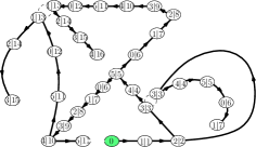
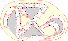
Figure 7: (a) The tree $\Theta(G)$ of geodesic edges of the galaxy of Fig. 2(a) after vertex splitting. (b) The colored cactus $\Gamma(G)$ obtained after cutting $\Theta(G)$ off $\mathcal{S}_{g}$: white faces are represented in yellow/lighter grey and the red curve is the boundary. Colors are indicated inside vertices, while the distance labels (or canonical corner labels) are written just outside.

The splitting of a vertex $v$ with two incoming geodesic edges consists in replacing $v$ by two new vertices, each carrying one incoming geodesic edge and the outgoing edge following it in clockwise direction around $v$. Let $\Theta(G)$ be the graph obtained by splitting vertices with two incoming geodesic edges and removing non-geodesic edges. Observe that the marked vertex $x_{0}$ has in-degree 1, so that it is not split and $x_{0}$ is a vertex of $\Theta(G)$.

Proposition 3

The graph $\Theta(G)$ is a tree and for each vertex $v$ of $\Theta(G)$, $\delta(v)$ is given by the distance to the marked vertex $x_{0}$ in $\Theta(G)$.

Proof

By construction each vertex $v$ except the marked one has indegree one in $\Theta(G)$. Moreover, if $v$ has label $\delta(v)=i$ ($i\geq 1$) the edge arriving in $v$ in $\Theta(G)$ is a geodesic edge from $G$: in particular it originates from a vertex $v^{\prime}$ with label $\delta(v^{\prime})=i-1$. This implies by induction on $\delta(v)$ that all vertices of $\Theta(G)$ are accessible from the marked vertex in this graph. Hence $\Theta(G)$ is a tree and $\delta$ is the distance in $\Theta(G)$. $\Box$

In particular the distance labels can be recovered from the (unlabeled) marked tree $\Theta(G)$.

Now assume that the galaxy $G$ is drawn on $\mathcal{S}_{g}$. Since $\Theta(G)$ is a tree, $\mathcal{S}_{g}\setminus\Theta(G)$ has one open boundary and its closure is a surface $\mathcal{S}^{\partial}_{g}$ of genus $g$ with one boundary (homeomorphic to a circle). Let $\Gamma(G)$ be the map induced by $G$ on $\mathcal{S}^{\partial}_{g}$: By construction $\Gamma(G)$ directly inherits from the faces and non-geodesic edges of $G$, while each geodesic edge of $G$ produces two boundary edges in $\Gamma(G)$ (a white and a black one, depending on the color of the incident face). The local analysis of the possible configurations around each non marked vertex of $G$ yields the three cases presented in Figure 8 and shows that each such vertex results in $\Gamma(G)$ into two or three vertices, among which exactly one has some incoming white boundary edges (the vertex represented by a square in each case of Figure 8). The marked vertex $x_{0}$ results in two vertices without incoming edges. Let us call active the vertices of $\Gamma(G)$ that have at least one incoming white boundary edge. In particular each non marked vertex of $G$ corresponds to one active vertex of $\Gamma(G)$.

        

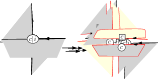
Figure 8: The three generic configurations in the construction of the induced map $\Gamma(G)$ on $\mathcal{S}^{\partial}_{g}=\overline{\mathcal{S}_{g}\setminus\Theta(G)}$: in-degree one; in-degree 2 with one geodesic incoming edge; in-degree 2 with two geodesic incoming edges. (In each case, the outgoing edges are represented as geodesic but could also be non-geodesic.)

Let $\mathcal{C}_{g}(\mu,\nu)$ denote the set of maps of genus $g$ with one boundary such that:

• (Face color condition) There are $m_{i}$ white faces of degree $(r+1)i$ and $n_{i}$ black faces of degree $(r+1)i$ for all $i$. There are three types of edges: internal edges that are incident to a black and a white face; white boundary edges that are oriented and have s white face on their right hand side; and black boundary edges that have a black face on their left-hand side.

• (Vertex color condition) All vertices are incident to the boundary, and have a color in $\{0,\ldots,r\}$ so that each (oriented) boundary edge $u\to v$ joins a vertex $u$ with color $c(u)$ to a vertex $v$ with color $c(v)=(c(u)\mod r+1)$.

• (Hurwitz condition) There are $d-1$ active vertices of each color (recall that a vertex is active if it has at least one incoming white boundary edge).

The following lemma is then a rephrasing of the previous discussion.

Lemma 4

The map $\Gamma(G)$ belongs to $\mathcal{C}_{g}(\mu,\nu)$.

Given a map $C$ with one boundary and an orientation of the edges of the boundary, a canonical corner labeling is a mapping $\delta$ from the set of boundary corners of $C$ into non-negative integers such that (a) the minimum label is $0$, (b) for each boundary edge $e=u\to v$, $\delta(c^{\prime})=\delta(c)+1$, where $c$ (resp. $c^{\prime}$) is the boundary corner incident to $e$ at $u$ (resp. at $v$). In particular for any galaxy $G$, the corner labeling of $\Gamma(G)$ inherited from the distance labeling on $G$ is canonical by construction. This construction is illustrated by Figure 7(b) (in the picture corner labels common to nearby corners are shared to limit cluttering).

Lemma 5

Each map $C\in\mathcal{C}_{g}(\mu,\nu)$ has a unique canonical corner labeling.

Proof

Choose an arbitrary corner $c$ on the boundary of $C$ and give it label 0. In view of Condition (b) above, the label of the next corner in clockwise direction around the boundary is either $1$ or $-1$ depending if the traversed edge is a white or a black boundary edge. All corner labels can be determined in this way and Condition (b) is satisfied on the edge closing the boundary cycle because there are equal numbers of black and white boundary edges (so that the $\pm 1$ walk giving labels automatically returns to zero when the boundary has been entirely traversed). As a result all corners get integer labels. Upon simultaneously shifting them so that the minimum is 0, the lemma is proved. $\Box$

The canonical corner labeling $\delta$ of a map $C\in\mathcal{C}_{g}(\mu,\nu)$ is coherent if for each vertex $u$ of $C$, all boundary corners of $u$ have the same label. In this case the corner labeling yields a vertex labeling called the coherent canonical labeling of $C$. The canonical labeling of Figure 7(b) is (by construction) coherent, as can be checked around the two active vertices of indegree 2, with labels 3 and 13 respectively. Let $\mathcal{C}^{c}_{g}(\mu,\nu)$ denote the set of maps of $\mathcal{C}_{g}(\mu,\nu)$ whose canonical corner labeling is coherent. In general not all maps of $\mathcal{C}_{g}(\mu,\nu)$ have a coherent canonical corner labeling, but this is the case in the genus zero case:

Proposition 4

Canonical corner labelings of maps in $\mathcal{C}_{0}(\mu,\nu)$ are coherent: $\mathcal{C}_{0}(\mu,\nu)=\mathcal{C}^{c}_{0}(\mu,\nu)$.

Proof

The only vertices of maps in $\mathcal{C}_{g}(\mu,\nu)$ that are incident to more than one boundary corner are the vertices gluing two white polygons. In particular each such map decomposes as a collection of components with simple boundaries glued by these vertices.

Now the maps in $\mathcal{C}_{0}(\mu,\nu)$ are planar and have only one boundary: their polygons thus form a tree-like structure (a kind of cactus). In particular each such map contains at least one component that is connected to the rest by only one vertex (a leaf polygon), and its canonical corner labeling is coherent if and only if the map in which this component is removed is. Upon pruning the map iteratively, the canonical corner labeling is seen to be coherent everywhere. $\Box$

Finally a map of $\mathcal{C}^{c}_{g}(\mu,\nu)$ is proper if the (common) color of its vertices with canonical label 0 is 0, and we denote by $\mathcal{C}^{0c}_{g}(\mu,\nu)$ the corresponding subset of $\mathcal{C}^{c}_{g}(\mu,\nu)$.

Proposition 5

The mapping $\Gamma$ is a bijection between the sets $\mathcal{H}_{g}(\mu,\nu)$ and ${\mathcal{C}}^{0c}_{g}(\mu,\nu)$.

This proposition is a direct consequence of the following two lemmas.

Lemma 6

The decomposition $G\to(\Theta(G),\Gamma(G))$ is injective.

Proof

The boundary of $\Gamma(G)$ forms a cycle with twice as many edges as there are edges in $\Theta(G)$: upon matching the marked vertex of $\Theta(G)$ with the marked vertex of $\Gamma(G)$ there is a unique way to glue $\Theta(G)$ on the boundary of $\Gamma(G)$ and recover $G$. $\Box$

Lemma 7

The canonical corner labels around the boundary of $\Gamma(G)$ encodes the tree $\Theta(G)$.

Proof

The counterclockwise sequence of labels around the boundary of $\Gamma(G)$ starting from the marked vertex $x_{0}$ is exactly the standard contour code of the plane tree $\Theta(G)$ [30, Chap. 5] (aka Dyck code, or discrete excursion encoding the tree). $\Box$

Proof (of Proposition 5)

The two lemmas above show that the mapping ${\Gamma}$ is injective. Given an element $C_{0}$ of $\mathcal{C}^{0c}_{g}(\mu,\nu)$, its sequence of canonical corner labels encodes a tree on which $C_{0}$ can be glued to form a map $G$ of genus $g$. This map is a galaxy of type $(\mu,\nu)$ in view of the face color and vertex color conditions on maps of $\mathcal{C}_{g}(\mu,\nu)$. The fact that $C_{0}$ is coherent allows to reconstruct a vertex labeling which coincide with the distance labeling on $G$. Finally the Hurwitz condition on maps of $\mathcal{C}_{g}(\mu,\nu)$ ensures that $G$ is a Hurwitz galaxy. $\Box$

The shift of a map $C\in{\mathcal{C}}^{c}_{g}(\mu,\nu)$ consists in adding one modulo $r+1$ to all colors. Recall that a map $C\in{\mathcal{C}}^{c}_{g}(\mu,\nu)$ is proper (that is, it belongs to $\mathcal{C}^{0c}_{g}(\mu,\nu)$) if the color of vertices with minimal label is 0.

Proposition 6

Each shift-equivalence class of maps of ${\mathcal{C}}^{c}_{g}(\mu,\nu)$ contains $r+1$ distinct maps, exactly one of which has a proper canonical corner labeling, that is, belongs to $\mathcal{C}^{0c}_{g}(\mu,\nu)$.

Proof

Shifting changes by one the (common) color of all the vertices that carry the minimum corner label: there are therefore at least $r+1$ distinct maps in a shift equivalence class. Moreover after $r+1$ shifts one returns to the original coloring so that there are exactly $r+1$ maps in each shift equivalence class, and exactly one of these maps has minimum label vertices of color 0. $\Box$

Corollary 8

The mapping $\Gamma$ is a bijection between the set $\mathcal{H}_{g}(\mu,\nu)$ of Hurwitz galaxies of genus $g$ and type $(\mu,\nu)$ and the set of shift equivalence classes of maps of ${\mathcal{C}}^{c}_{g}(\mu,\nu)$.

4.2 Simplifying cacti to get Hurwitz mobiles

The graph $\Phi(G)$ constructed from a galaxy $G$ can be seen as the retractation of $\Gamma(G)$: More precisely, given a Hurwitz galaxy $G$, observe that the rules of Figure 4(a) and 4(b) can be equivalently applied to $\Gamma(G)$ instead of $G$ to construct $\Phi(G)$. Indeed the non-geodesic edges of $G$ to which the rule of Figure 4(a) applies exactly correspond to the internal edges of $\Gamma(G)$, while the vertices that are split by the rule of Figure 4(b) correspond to the vertices incident to two white faces in $\Gamma(G)$. The fact that $\Gamma(G)\in{\mathcal{C}}^{c}_{g}(\mu,\nu)$ directly implies that $\Phi(G)$, as a graph, is an edge-labeled Hurwitz mobiles of type $(\mu,\nu)$ and excess $2g$ (in particular the Hurwitz condition on maps of $\mathcal{C}_{g}(\mu,\nu)$ implies that the edge labels in the retract are all distinct). We can thus define the retractation map $\Pi$ from ${\mathcal{C}_{g}(\mu,\nu)}$ to $\mathcal{M}_{g}(\mu,\nu)$ by the rules of Figure 4(a) and (b).

For the retractation of $\Gamma(G)$ to be reversible, one should however be able to recover the map structure: the cyclic order of edges around the nodes of polygons is fixed. As opposed to this, we have defined Hurwitz mobiles as graphs (that is, without specifying an embedding). However observe that the order of edges around nodes of the polygons of the retractation is determined by the fact that on each node of a white (resp. black) polygon, the edge labels are increasing in clockwise (resp. counterclockwise) order. Let us define the canonical embedding of a Hurwitz mobile as the unique embedding in a closed compact surface induced by these local conditions. We say that a Hurwitz mobile with excess $2g$ has genus $g$ if this canonical embedding is an embedding in $\mathcal{S}_{g}$. Of course a Hurwitz mobile with excess $0$ has always genus $0$, but for $g\geq 1$ Hurwitz mobiles with excess $2g$ may have a genus smaller than $g$, (in which case their canonical embedding has several faces). Let $\tilde{{H}}_{g}(\mu,\nu)$ be the subset of ${H}_{g}(\mu,\nu)$ consisting of Hurwitz mobiles that have genus $g$.

Proposition 7

The retract $\Pi$ is a bijection between ${\mathcal{C}}_{g}(\mu,\nu)$ and the set of $\mathcal{M}^{1}_{g}(\mu,\nu)$ of Hurwitz mobiles with excess $2g$ and genus $g$ and type $(\mu,\nu)$. Moreover the shifts on $\mathcal{C}_{g}(\mu,\nu)$ and on $\mathcal{M}^{1}_{g}(\mu,\nu)$ are equivalent operations: for any $C\in\mathcal{C}_{g}(\mu,\nu)$, $\Pi(\sigma(C))=\sigma(\Pi(C))$.

Proof

As already discussed $R$ is a mapping from ${\mathcal{C}}_{g}(\mu,\nu)$ to ${\mathcal{M}}^{1}_{g}(\mu,\nu)$. Conversely given a Hurwitz mobile $M$, one associates to each $i$-gon of $M$ a face of degree $(r+1)i$ divided into $r+1$ subregions (the interior of the polygon and $i$ subregions with boundary edges $\to 0\to 1\to\ldots\to r\to$ associated to the $i$ nodes of the $i$-gon). Then there is a unique way to embed locally each white (resp. black) polygon and its incident edges in the associated white (resp. black) face so that

• White (resp. black) polygons are drawn clockwise (resp. counterclockwise).

• The labels of edges incident to a given node on a white (resp. black) polygon increase in clockwise (resp. counterclockwise) direction between the two arcs incident to this node.

• Each zero weight half-edge with color $c^{\prime}$ reaches a boundary vertex with color $c^{\prime}$ incident to the same subregion as its origin.

• Each non-zero weight half-edge with color $c^{\prime}$ reaches the middle of an edge with colors $c\to c^{\prime}$, with $c^{\prime}=c+1\mod r+1$.

The resulting faces can then be coherently glued together according to the edges of $M$, and the result is a element of ${\mathcal{C}}^{1}_{g}(\mu,\nu)$ since all local conditions are satified. Finally the shift operation on $\mathcal{M}_{g}(\mu,\nu)$ is a direct translation through the retract of the shift on $\mathcal{C}_{g}(\mu,\nu)$. $\Box$

To combine this proposition with Proposition 5 we need a last definition: an edge-labeled Hurwitz mobile of genus $g$ is coherent if the canonical corner labeling of the associated map of $\mathcal{C}_{g}(\mu,\nu)$ is. Let $\mathcal{M}^{1c}_{g}(\mu,\nu)$ denote the set of coherent edge-labeled Hurwitz mobiles of excess $2g$ and genus $g$ and type $(\mu,\nu)$. According to the previous remarks, we have finally proved the following theorem.

Theorem 4.1

The mapping $M$ is a bijection between Hurwitz galaxies and shift-equivalence classes of coherent edge-labeled Hurwitz mobiles with the same genus and type. As a consequence, Hurwitz numbers of genus $g$ count shift-equivalence classes of coherent Hurwitz mobiles of genus $g$:

$$h^{\bullet}_{g}(\mu,\nu)=\frac{1}{m+n-1+2g}\;|{\mathcal{M}}^{1c}_{g}(\mu,\nu)|$$

Proposition 4 shows that $\mathcal{M}^{1c}_{0}(\mu,\nu)=\mathcal{M}_{0}(\mu,\nu)$, so that Theorem 4.1 implies in particular Theorem 2.1.

5 Concluding remarks

1) The mapping $\Gamma$ that we use in the first step of our proof can be viewed as a reformulation of a special case of the Bouttier-Di Francesco-Guitter construction [6] in terms of vertex splitting [3, 2]. Our main contribution here is to identify the image of $\Gamma$ and show that it can be mapped (through $\Pi$) onto a set of well characterized Hurwitz mobiles.

2) The construction in fact holds more generally for non-Hurwitz galaxies where instead of $r$ simple branched points (with $d-1$ preimages), one requires $s$ branched points with respectively $d-r_{i}$ preimages with $\sum_{i=1}^{s}r_{i}=r$. The resulting mobiles are slightly more complex but again in the planar case explicit formulas can be found for the corresponding double $s$-eulerian numbers in the terminology of Goulden and Jackson [14].

3) The specialization of the bijection to the case $\mu=\nu=1^{n}$ is already non trivial: let us call simple coverings of size $n$ the corresponding branched coverings of the sphere by itself with $2n-2$ critical values that are all simple, and simple galaxies the corresponding galaxies. Theorem 2.1 gives a bijection between simple galaxies of size $n$ and a variant of Cayley trees, namely edge-labeled Cayley trees with exactly one leaf incident to each inner vertex (from Cayley’s formula one immediately deduce that these trees are counted by the formula $n^{n-3}(2n-2)!/(n-1)!$). In view of the construction of the bijection, the oriented pseudo-distance in the galaxy representing a covering can be read on a canonical embedding in $\mathbb{Z}$ of the associated tree induced by its the canonical corner labeling. The variation between successive corner labels associated to two successive edges of the tree along a branch are easily seen to be symetric random non zero integer variables taken uniformly in the interval $[-n+1,n-1]$. One can thus expect, in analogy with the many results of convergence of embedded trees to the Brownian snakes [23, 22] that upon scaling the embedding support by a factor $n^{-5/4}$, the resulting random embedded trees converge to the Brownian snake. As a consequence, we expect that refinements of the technics of [23, 22] allow to prove that:

the length $L_{n}$ of the shortest oriented path between two random vertices of uniform random simple galaxy of size $n$ satisfies $L_{n}\cdot n^{-5/4}\to cte\cdot\mathcal{L}$ where $\mathcal{L}$ is the distance between two random points in the Brownian map (see e.g. [8]).

We then conjecture that, as the size tends to infinity, the $n^{-5/4}$ rescaled oriented pseudo-distances between the various pairs of points of a same random simple galaxy become asymptotically symmetric, and coincide a.s. with the $n^{-1/4}$ rescaled non-oriented distances on the same galaxy up to a constant (non random) stretch factor. We currently have no idea on how to prove such a result, but it would imply that $n^{-1/4}$ rescaled uniform random simple galaxies of size $n$ converge to the Brownian map in the same sense as uniform random quadrangulations do [21, 24]. This would be in agreement with the general (somewhat vague) assertion that uniform random branched coverings of the sphere fall in the same universality class as uniform random planar quadrangulations, and that they both are natural discrete models of pure two-dimensional quantum geometries (see e.g. [31]).

4) The graph metric defined by uniform random simple galaxies of size $n$ is a particular set of random discrete metric space associated to uniform random simple coverings of size $n$. As mentioned at the end of Section 2.1, there are other possible choices of curves on the image sphere whose preimage yield different families of maps in bijection with simple coverings: an example is given by the increasing quadrangulations that arise as preimages of a bundle of parallel edges separating the critical values [9]. We believe that the uniform distribution on any such resulting family of maps induces, upon considering the graph metric on it, a family of random discrete metric spaces that also converges upon scaling to the Brownian map. A very appealing approach to such a universality result would be to find a way to relate these discrete metrics to the complex structures of the underlying simple coverings.

Acknowledgements. M. Kazarian and D. Zvonkine are warmly thanked for sharing their conjectures on double Hurwitz numbers and for interesting discussions. The authors acknowledge support of ERC under grant StG 208471.

References

- [1] M. Albenque and D. Poulalhon. A generic method for bijections between blossoming trees and planar maps. Electr. J. Combinatorics, 2014.
- [2] O. Bernardi and C. Chapuy. A bijection for covered maps, or a shortcut between harer-zagier’s and jackson’s formulas. Journal of Combinatorial Theory - Series A, 118(6):1718, 1748 2011.
- [3] O. Bernardi and E. Fusy. Unified bijections for maps with prescribed degrees and girth. Journal of Combinatorial Theory - Series A, 119(6):1351–1387, 2012.
- [4] G. Borot, B. Eynard, M. Mulase, and B. Safnuk. A matrix model for simple Hurwitz numbers, and topological recursion. Journal of Geometry and Physics, 61(2):522–540, 2011.
- [5] M. Bousquet-Mélou and G. Schaeffer. Enumeration of planar constellations. Advances in Applied Mathematics, 24(4):337–368, 2000.
- [6] J. Bouttier, P. Di Francesco, and E. Guitter. Planar maps as labeled mobiles. Electron. J. Combin., 11(1):# 69, 2004.
- [7] R. Cavalieri, P. Johnson, and H. Markwig. Tropical hurwitz numbers. JACO, 2010.
- [8] P. Chassaing and G. Schaeffer. Random planar lattices and integrated superbrownian excursion. Probability Theory and Related Fields, 128(2):161–212, 2004.
- [9] E. Duchi, D. Poulalhon, and G. Schaeffer. Uniform random sampling of simple branched coverings of the sphere by itself, chapter 21, pages 294–304. 2014.
- [10] P. Dunin-Barkowski, M. Kazarian, N. Orantin, S. Shadrin, and L. Spitz. Polynomiality of hurwitz numbers, bouchard-mariño conjecture, and a new proof of the elsv formula. arXiv:1307.4729, 2013.
- [11] T. Ekedahl, S. Lando, M. Shapiro, and A. Vainshtein. Hurwitz numbers and intersections on moduli spaces of curves. Inventiones mathematicae, 146(2):297–327, 2001.
- [12] B. Eynard. Counting Surfaces: Combinatorics, Matrix Models, Algebraic Geometry. Birkhäuser, 2014.
- [13] I. Goulden and D. Jackson. Transitive factorisations into transpositions and holomorphic mappings on the sphere. Proceedings of the American Mathematical Society, 125(1):51–60, 1997.
- [14] I.P. Goulden and Jackson D.M. The KP hierarchy, branched covers, and triangulations. Advances in Mathematics, 219:932–951, 2008.
- [15] I.P. Goulden, D.M. Jackson, and R. Vakil. Towards the geometry of double hurwitz numbers. Adv. Math., 198(1):43–92, 2005.
- [16] P. Johnson. Hurwitz numbers, ribbon graphs, and tropicalization. In Tropical geometry and integral systems, number 580 in Comtemp. Math., pages 55–72. Amer. Math. Soc., Providence, RI, 2012. arXiv:1303.1543.
- [17] P. Johnson. Double hurwitz numbers via the infinite wedge. Transactions of the AMS, 2014. to appear, arXiv:1008.3266.
- [18] M. Kazarian. Private communication. 2014.
- [19] M. Kazarian and S. Lando. An algebro-geometric proof of witten’s conjecture. J. Amer. Math. Soc., 20(4):1079–1089, 2007.
- [20] S.K. Lando and A. K. Zvonkin. Graphs on Surfaces and their applications. Encyclopaedia of Mathematical Sciences. Springer-Verlag, 2004.
- [21] J.-F. Le Gall. Uniqueness and universality of the brownian map. arXiv preprint arXiv:1105.4842, to appear in Ann. Proba., 2011.
- [22] J.-F. Marckert and G. Miermont. Invariance principles for random bipartite planar maps. The Annals of Probability, 35(5):1642–1705, 2007.
- [23] G. Miermont. Invariance principles for spatial multitype galton-watson trees. Ann. Inst. Henri Poincaré (B), 44:1128–1161, 2008.
- [24] G. Miermont. The brownian map is the scaling limit of uniform random plane quadrangulations. arXiv preprint arXiv:1104.1606, to appear in Acta Math., 2011.
- [25] S. M. Natanzon and A. V. Zabrodin. Toda hierarchy, hurwitz numbers and conformal dynamics. arXiv:1302.7288.
- [26] A. Okounkov. Toda equations for Hurwitz numbers. Math. Res. Lett., 7(4):447–453, 2000.
- [27] A. Okounkov and R. Pandharipande. Gromov-Witten theory, Hurwitz numbers, and matrix models, i. arXiv preprint math/0101147, 2001.
- [28] G. Schaeffer. Conjugaison d’arbres et cartes combinatoires. PhD thesis, Université Bordeaux 1, 1998.
- [29] S. Shadrin, M. Shapiro, and A. Vainshtein. Chamber behavior of double hurwitz numbers in genus 0. Adv. Math., 217(1):79–96, 2008.
- [30] R. P. Stanley. Enumerative combinatorics. Vol. 2, volume 62 of Cambridge Studies in Advanced Mathematics. Cambridge University Press, 1999.
- [31] D. Zvonkine. Enumeration of ramified coverings of the sphere and 2-dimensional gravity. arXiv preprint math/0506248, 2005.