Relational Mechanics as a gauge theory

Abstract

Absolute space is eliminated from the body of mechanics by gauging translations and rotations in the Lagrangian of a classical system. The procedure implies the addition of compensating terms to the kinetic energy, in such a way that the resulting equations of motion are valid in any frame. The compensating terms provide inertial forces depending on the total momentum ${\bf P}$, intrinsic angular momentum ${\bf J}$ and intrinsic inertia tensor ${\bf I}$. Therefore, the privileged frames where Newton’s equations are valid (Newtonian frames) are completely determined by the matter distribution of the universe (Machianization). At the Hamiltonian level, the gauge invariance leads to first class constraints that remove those degrees of freedom that make no sense once the absolute space has been eliminated. This reformulation of classical mechanics is entirely relational, since it is a dynamics for the distances between particles. It is also Machian, since the rotation of the rest of the universe produces centrifugal effects. It then provides a new perspective to consider the foundational ideas of general relativity, like Mach’s principle and the weak equivalence principle. With regard to the concept of time, the absence of an absolute time is known to be a characteristic of parametrized systems. Furthermore, the scale invariance of those parametrized systems whose potentials are inversely proportional to the squared distances can be also gauged by introducing another compensating term associated with the intrinsic virial $G$ (shape-dynamics).

I Introduction

Newton’s mechanics describes particle motions relative to external absolute space and time. The evolution of an isolated system of $N$ particles is determined by a set of independent initial positions and velocities, whose sole ambiguity lies in the choice of the inertial frame we use to express the initial configuration. Thus the system has $3N$ degrees of freedom. The quality of inertial is conferred by the state of motion of the frame relative to the absolute space. This approach was criticized by Leibniz and Mach, who claimed for a dynamics of relations among particles without any reference to external non-material entities Alexander ; Mach . Mach’s ideas guided Einstein in its way towards general relativity: “… it is contrary to the mode of thinking in science to conceive of a thing (the space-time continuum) which acts itself, but which cannot be acted upon. This is the reason why E. Mach was led to make the attempt to eliminate space as an active cause in the system of mechanics” Einstein . During the last century, different strategies have been tried to formulate a relational mechanics in agreement with Mach’s thought. Most of them were based on a reformulation of the kinetic energy as a sum of “interaction” terms decreasing with the distance Reissner ; Schrodinger ; Barbour75 ; Barbour77 ; Barbour95 . However these approaches predicted non-observed anisotropies of the inertia Barbour77 , and could not explain the undisputable success of Newton’s theory. The idea that the Lagrangian should exhibit gauge invariance under the Galilean group was introduced in References Barbour77, and Barbour82, . This requirement guarantees the abolition of the absolute space, since any frame becomes valid to apply the dynamical equations; but it does not completely prescribe the Lagrangian. In Ref. Barbour82, a given Lagrangian is gauged by replacing its measure (kinetic energy) with a measure defined in the space of orbits (each orbit represents a set of configurations that are equivalent under gauge transformations). The measure between two orbits, or intrinsic differential, results from minimizing the original measure between configurations belonging to the involved orbits (“best matching” Barbour03 ). The so obtained gauge invariant dynamics is left with those solutions to the original Lagrangian having vanishing momentum and angular momentum. This strategy has been improved in Ref. Gryb, , where it is extended to arbitrary symmetry groups and finite transformations, on the basis of comparing with Yang-Mills gauge theories. In this article we will follow the approach of gauging a well established Lagrangian: the one for standard Newton’s mechanics. Instead of defining a measure between orbits, we will introduce counterterms in the kinetic energy to compensate the changes of Newton’s kinetic energy under gauge transformations. In this way, we will get an explicitly gauge invariant Lagrangian leading to equations of motion that are valid in any frame.

Newton’s laws are invariant under rigid (time-independent) time translations, and space translations and rotations of particle’s positions $\mathbf{r}_{i}$:

time translation: $$t~{}\longrightarrow~{}t~{}+~{}\epsilon~{},$$ (1)

space translation: $$\mathbf{r}_{i}~{}\longrightarrow~{}\mathbf{r}_{i}~{}+~{}\mathbf{\xi}~{},$$ (2)

rotation: $$\mathbf{r}_{i}~{}\longrightarrow~{}\mathbf{A\cdot r}_{i}~{},$$ (3)

where $\mathbf{A}$ is an orthogonal matrix. If the rotation is infinitesimal, it becomes

$$\mathbf{r}_{i}~{}\longrightarrow~{}\mathbf{r}_{i}~{}+\mathbf{\alpha}~{}\times~{}\mathbf{r}_{i}~{},$$ (4)

where $\mathbf{\alpha}$ is a vector directed along the axis of rotation, whose infinitesimal modulus is the angle of rotation. Besides, Newton’s laws are invariant under Galileo transformations,

$$\text{Galileo transformation: \ \ \ \ \ \ \ \ \ }\mathbf{r}_{i}~{}\longrightarrow~{}\mathbf{r}_{i}~{}+~{}\mathbf{V}t~{},$$ (5)

which constitute a particular case of local (time-dependent) space translations: those having $\mathbf{\xi}(t)=\mathbf{V}t$ .

Transformations (1-3) and (5) constitute the Galilean group of Newton’s mechanics. In Newton’s mechanics, absolute space and time are represented by the privileged family of inertial frames and clocks, which relate each other through the transformations of the Galilean group. The abolition of absolute space then calls for the elimination of privileged frames: the dynamics of relations must be governed by laws to be applied in any frame. This goal can be attained by building the Mechanics as a gauge theory of the Galilean group. To turn the Galilean group into a gauge group means to succeed in becoming local those already existing rigid symmetries. If so, not only rigid rotations will be allowed but any time-dependent rotation too; not only Galileo transformations will leave invariant the equations of motion but any time-dependent space translation too. The absolute time would be eliminated as well, since gauging the time translation implies that the parameter $t$ can be changed in an arbitrary way: $t~{}\longrightarrow~{}t~{}+~{}\epsilon(t)$; thus, the time parameter would become physically irrelevant. In sum, the dynamics of relations calls for Lagrangians that are invariant under arbitrary time-dependent rotations and translations together with arbitrary redefinitions of the time parameter. In such case, no privileged frames and clocks will remain in the formulation of mechanics, what is the mark of Relational Mechanics. Since Galileo transformations will be subsumed in the subgroup of local translations, it results that the gauge group of Relational Mechanics is composed of transformations (1-3). This gauge group has been called Leibniz group in Ref. Barbour77, (see also Ref. Ehlers, ).

A typical feature of gauge theories is the existence of constraints among the canonical variables. This means that not all the variables represent genuine degrees of freedom. In particular, by gauging translations and rotations the system of $N$ particles is left with $3N-6$ degrees of freedom. The dynamics of relations has less degrees of freedom than Newton’s dynamics because evolutions consisting in rigid translations and rotations means nothing in Relational Mechanics. The redundant variables can be frozen by fixing the gauge. In Relational Mechanics this procedure is equivalent to choose a frame. As we will show, Relational Mechanics contains frames where Newton’s equations are valid. But such frames are determined by the matter distribution of the universe, as required by Mach.

In Section II we obtain a Lagrangian that is invariant under local translations and rotations. We study the constraints and gauge fixing conditions associated with this Lagrangian. In Section III we obtain the relational equations of motion, and show the existence of frames where Newton’s equations are valid. We apply these equations to the case of Newton’s bucket to show that the centrifugal effect would disappear if the rest of the universe were absent. We compare this result with the nature of the centrifugal effect in general relativity. We also discuss the status of the weak equivalence principle. In Section IV we explain how the absolute time is eliminated by parametrizing the system. In Section V we show that the scale invariance can also be gauged by including a counterterm associated with the intrinsic virial function (the scale invariance requires potentials that are inversely proportional to the squared distances). In Section VI we display the conclusions.

II Gauging translations and rotations

As a first step in the way to its relational formulation, Mechanics should be reduced to a dynamics of relative positions

$$\mathbf{r}_{ij}~{}\doteq~{}\mathbf{r}_{i}-\mathbf{r}_{j}~{}.$$ (6)

This goal can be reached by gauging the translations; this means the process of becoming local (dependent on time) the rigid symmetry (2). In fact, velocities are not invariant under local translations but change as

$$\mathbf{v}_{k}~{}\longrightarrow~{}\mathbf{v}_{k}+{\dot{\mathbf{\xi}}}(t)~{}.$$ (7)

Therefore, a Lagrangian invariant under local translations is expected to depend just on relative velocities $\mathbf{v}_{ij}={\dot{\mathbf{r}}}_{ij}$.

The process of gauging a rigid symmetry in gauge theories involves the introduction of gauge fields to compensate the (bad) behavior of derivatives under local transformations. In a more technical language, one introduces a connection to make the derivatives behave in a covariant way; i.e., thanks to the compensating terms the derivatives behave in the same way both under local and rigid transformations. In gauge theory, the dynamics is constrained by relations emerging from the local symmetry the fields obey. The constrains imply that not all the fields are genuine degrees of freedom, since their initial values cannot be chosen in a completely free way. A remarkable feature of gauge fields is that they mediate interactions by carrying energy-momentum at a finite propagation velocity. Instead, classical mechanics describes interactions through potentials $V(r_{ij})$ depending just on the distances between particles; it is the realm of instantaneous interactions at a distance. As a consequence, the degrees of freedom associated with the external space and time can be eliminated without introducing new fields, but just resorting to the same dynamical variables we started from. This can be made by providing the Lagrangian with compensating terms depending on positions and velocities. Notice that $V(r_{ij})$ is already a gauge invariant quantity. Therefore, mechanics will become relational if the kinetic energy in the Lagrangian becomes a gauge invariant quantity. Newton’s kinetic energy is not invariant under local translations $\mathbf{\xi}(t)$; if $\mathbf{\xi}$ is infinitesimal, it changes as

$$\sum\limits_{k}\frac{m_{k}}{2}~{}\delta(\mathbf{v}_{k}\cdot\mathbf{v}_{k})~{}=\sum\limits_{k}m_{k}~{}\mathbf{v}_{k}\cdot\delta\mathbf{v}_{k}~{}=~{}{\dot{\mathbf{\xi}}}\cdot\sum\limits_{k}m_{k}~{}\mathbf{v}_{k}=~{}{\dot{\mathbf{\xi}}}\cdot\mathbf{P}~{}.$$ (8)

Remarkably, the square total momentum $\mathbf{P}$ changes essentially in the same way:

$$\delta(\mathbf{P}\cdot\mathbf{P})~{}=~{}2~{}\mathbf{P}\cdot\delta\mathbf{P}=~{}2~{}\mathbf{P}\cdot~{}\sum\limits_{k}m_{k}~{}{\dot{\mathbf{\xi}}}~{}=~{}2M{\dot{\mathbf{\xi}}}\cdot\mathbf{P}~{}.$$ (9)

So, we can gauge the translations by compensating the kinetic energy with the counterterm $\mathbf{P}\cdot\mathbf{P}/(2M)$. The gauged kinetic energy turns out to be the kinetic energy in a frame where the center of mass is at rest; it gets the form of an intrinsic kinetic energy:

$$\sum\limits_{i<j}\frac{m_{i}m_{j}}{2M}~{}\mathbf{v}_{ij}\cdot\mathbf{v}_{ij}~{}=\sum\limits_{k}\frac{m_{k}}{2}~{}\mathbf{v}_{k}\cdot\mathbf{v}_{k}~{}-~{}\frac{\mathbf{P}\cdot\mathbf{P}}{2M}~{}=\sum\limits_{k}\frac{m_{k}}{2}~{}\left(\mathbf{v}_{k}-\frac{\mathbf{P}}{M}\right)\cdot\left(\mathbf{v}_{k}-\frac{\mathbf{P}}{M}\right)~{}.$$ (10)

So, the Lagrangian

$$L~{}=~{}\sum\limits_{i<j}\,\frac{m_{i}~{}m_{j}}{2M}~{}\mathbf{v}_{ij}\cdot\mathbf{v}_{ij}~{}-~{}V(r_{ij})~{}$$ (11)

is invariant under local translations. Remarkably, in the kinetic energy (10) the derivative of the position $\mathbf{v}_{k}=d\mathbf{r}_{k}/dt$ is accompanied by a compensating term $\mathbf{P}/M$, in such a way that the complete expression is invariant not only under rigid translations but under local translations too. In fact,

$$\mathbf{v}_{k}-\frac{\mathbf{P}}{M}\longrightarrow\mathbf{v}_{k}+{\dot{\mathbf{\xi}}}-\frac{\mathbf{1}}{M}\sum\limits_{i}m_{i}~{}(\mathbf{v}_{i}+{\dot{\mathbf{\xi}})}=\mathbf{v}_{k}-\frac{\mathbf{P}}{M}~{}.$$ (12)

It could be said that the compensating term $\mathbf{P}/M$ “covariantizes” the time derivative under local translations.

We will follow the same strategy for gauging the rotations. Lagrangian (11) is invariant under rigid rotations. Instead, local infinitesimal rotations produce the change

$$\delta(\mathbf{v}_{ij}\cdot\mathbf{v}_{ij})~{}=~{}2~{}\mathbf{v}_{ij}\cdot\delta\mathbf{v}_{ij}=~{}2~{}\mathbf{v}_{ij}\cdot\frac{d}{dt}(\mathbf{\alpha}~{}\times~{}\mathbf{r}_{ij})=~{}2~{}\mathbf{v}_{ij}\cdot(\dot{\mathbf{\alpha}}\times~{}\mathbf{r}_{ij})~{}=~{}2~{}\dot{\mathbf{\alpha}}\cdot(\mathbf{r}_{ij}~{}\times~{}\mathbf{v}_{ij})~{},$$ (13)

which makes the kinetic energy vary in

$$\sum\limits_{i<j}\,\frac{m_{i}~{}m_{j}}{2M}~{}\delta(\mathbf{v}_{ij}\cdot\mathbf{v}_{ij})~{}=~{}\dot{\mathbf{\alpha}}\cdot~{}\mathbf{J}~{},$$ (14)

where $\mathbf{J}$  is the intrinsic angular momentum or spin, which is invariant under local translations:

$$\mathbf{J}~{}\ \doteq~{}\ \sum\limits_{i<j}\,\frac{m_{i}~{}m_{j}}{M}~{}\mathbf{r}_{ij}\times\mathbf{v}_{ij}~{}=~{}\sum\limits_{k}\,m_{k}~{}\mathbf{r}_{k}\times\mathbf{v}_{k}-\mathbf{R}\times\mathbf{P}~{}=~{}\sum\limits_{k}\,m_{k}~{}(\mathbf{r}_{k}-\mathbf{R})\times\left(\mathbf{v}_{k}-\frac{\mathbf{P}}{M}\right)~{}$$ (15)

($\mathbf{R}$ is the center-of-mass position). To compensate the behavior (14) we will provide the kinetic energy with a counterterm quadratic in $\mathbf{J}$. This term has to be invariant under rigid translations and rotations, so we write it as $(1/2)\,\mathbf{J}\cdot\mathbf{I}^{-1}\cdot\mathbf{J}$, where $\mathbf{I}^{-1}$ is some symmetric tensor depending only on relative positions (then, $\dot{\mathbf{\alpha}}$ does not appear in the local rotation of $\mathbf{I}^{-1}$). Under local rotations the counterterm varies in

$$\frac{1}{2}~{}\delta(\mathbf{J}\cdot\mathbf{I}^{-1}\cdot\mathbf{J)~{}}\ =\ ~{}\delta\mathbf{J}\cdot\mathbf{I}^{-1}\cdot\mathbf{J}~{},$$ (16)

where we only use those terms in $\delta\mathbf{J}$ that are proportional to $\dot{\mathbf{\alpha}}$, since rigid rotations do not change the counterterm:

$$\delta\mathbf{J}\ =\ \sum\limits_{i<j}\frac{m_{i}~{}m_{j}}{M}~{}\mathbf{r}_{ij}~{}\times(\dot{\mathbf{\alpha}}\times~{}\mathbf{r}_{ij})+...$$ (17)

Therefore

$$\delta\mathbf{J}\ =\ \sum\limits_{i<j}\frac{m_{i}~{}m_{j}}{M}~{}[r_{ij}^{2}~{}\dot{\mathbf{\alpha}}-\mathbf{r}_{ij}~{}(\dot{\mathbf{\alpha}}\cdot\mathbf{r}_{ij})]~{}\ +\ ...~{}\ =\ ~{}\dot{\mathbf{\alpha}}\cdot\mathbf{I}\ +\ ...$$ (18)

where $\mathbf{I}$ is the intrinsic inertia tensor,

$$\mathbf{I}~{} \doteq ~{}\sum\limits_{i<j}\frac{m_{i}~{}m_{j}}{M}~{}[r_{ij}^{2}~{}\mathbf{1}-\mathbf{r}_{ij}\otimes\mathbf{r}_{ij}]\ =~{}\sum\limits_{k}m_{k}\,(r_{k}^{2}~{}\mathbf{1}-\mathbf{r}_{k}\otimes\mathbf{r}_{k})-M\,(R^{2}~{}\mathbf{1}-\mathbf{R}\otimes\mathbf{R})\$$

$$= ~{}\sum\limits_{k}m_{k}\,\left[|\mathbf{r}_{k}-\mathbf{R}|^{2}~{}\mathbf{1}-(\mathbf{r}_{k}-\mathbf{R})\otimes(\mathbf{r}_{k}-\mathbf{R})\right]~{},$$ (19)

which is just the inertia tensor relative to the center of mass. Replacing the result (18) in Eq. (16) we reproduce the behavior (14) of the intrinsic kinetic energy under local rotations. Therefore, not only translations but also rotations are gauged if the Lagrangian is taken to be

$$L~{}=~{}\sum\limits_{i<j}\frac{m_{i}~{}m_{j}}{2M}~{}\mathbf{v}_{ij}\cdot\mathbf{v}_{ij}~{}-~{}\frac{1}{2}~{}\mathbf{J}\cdot\mathbf{I}^{-1}\cdot\mathbf{J}~{}-~{}V(r_{ij})~{}.$$ (20)

Lagrangian (20) was introduced by Lynden-Bell in References Lynden92, ; Lynden95, ; Katz95, ; the counterterms were there obtained by looking for the minimum value the kinetic energy can reach under finite local translations and rotations. Such a minimum is reached for the values $\dot{\mathbf{\xi}}=\mathbf{P}/M$ and $\dot{\mathbf{\alpha}}=\mathbf{I}^{-1}\cdot\mathbf{J}$. In fact, it is remarkable that Lagrangian (20) can be rewritten as

$$L~{}=~{}\sum\limits_{k}\frac{m_{k}}{2}~{}\left|\mathbf{v}_{k}-\frac{\mathbf{P}}{M}-(\mathbf{I}^{-1}\cdot\mathbf{J})\times(\mathbf{r}_{k}-\mathbf{R})\right|^{2}-~{}V(r_{ij})~{}$$ (21)

(Hints: use $\sum\limits_{k}m_{k}~{}\mathbf{r}_{k}\times\mathbf{v}_{k}-\mathbf{R}\times\mathbf{P}=\mathbf{J}$; prove $\sum\limits_{i<j}m_{i}m_{j}~{}\mathbf{r}_{ij}\otimes\mathbf{r}_{ij}~{}/M=\sum\limits_{k}m_{k}~{}(\mathbf{r}_{k}-\mathbf{R})\otimes(\mathbf{r}_{k}-\mathbf{R})$). Although Lagrangian (20) describes the dynamics in terms of relative positions and velocities, it is still a function of individual positions and velocities because the relative positions cannot be considered as independent variables.

II.1 Constraints

Gauge invariance implies constraints among the momenta. The conjugate momenta coming from the Lagrangian (20) are

$$\mathbf{p}_{k}\ =\ m_{k}\ \left[\mathbf{v}_{k}-\frac{\mathbf{P}}{M}-(\mathbf{I}^{-1}\cdot\mathbf{J})\times(\mathbf{r}_{k}-\mathbf{R})\right]$$ (22)

(Hint: in Eq. (20) use the result $\partial J_{\mu}/\partial v_{k}^{\nu}=\epsilon_{\mu\lambda\nu}~{}m_{k}\ (\mathbf{r}_{k}-\mathbf{R})^{\lambda}$). Then, the momenta look like conventional momenta for particles whose velocities have been diminished by the motion of a rigid body that accompanies the center of mass and rotates with a time dependent angular velocity $\mathbf{I}^{-1}\cdot\mathbf{J}$, which is the mean angular velocity of the system. Moreover, $\mathbf{p}_{k}$ behaves as a vector not only under rigid rotations but under local rotations too; such a property is guaranteed by the compensating terms in Eq. (22) (to prove it, use Eq. (18)).

The momenta accomplish the constraint equations

$$\mathcal{P}\,\doteq\,\sum\limits_{k}~{}\mathbf{p}_{k}\,=\,0~{},\hskip 50.58878pt\mathcal{J}\,\doteq\,\sum\limits_{k}~{}\mathbf{r}_{k}\times\mathbf{p}_{k}\,=\,0~{}.$$ (23)

The first one is trivial because $\sum m_{k}(\mathbf{v}_{k}-\mathbf{P}/M)=0$ and $\sum m_{k}(\mathbf{r}_{k}-\mathbf{R})=0$. To prove the second one, we will use that $m_{k}(\mathbf{r}_{k}-\mathbf{R})=\sum\limits_{j}m_{k}m_{j}~{}\mathbf{r}_{kj}/M$; then

$$\mathcal{J\ } = \mathcal{\ }\sum\limits_{k}~{}\mathbf{r}_{k}\times\mathbf{p}_{k}\mathcal{\ }=\mathcal{\ }\sum\limits_{k}m_{k}~{}\mathbf{r}_{k}\times\left[\mathbf{v}_{k}-\frac{\mathbf{P}}{M}-(\mathbf{I}^{-1}\cdot\mathbf{J})\times(\mathbf{r}_{k}-\mathbf{R})\right]$$ (24)

$$= \mathcal{\ }\sum\limits_{k}m_{k}~{}\mathbf{r}_{k}\times\mathbf{v}_{k}\ -\ \mathbf{R}\times\mathbf{P}\ -\ \sum\limits_{k,\ j}\frac{m_{k}\,m_{j}}{M}~{}\mathbf{r}_{k}\times\left[(\mathbf{I}^{-1}\cdot\mathbf{J})\times\mathbf{r}_{kj}\right]\mathcal{\ }=\mathcal{\ }\mathbf{J}\ -\ \sum\limits_{i<j}\frac{m_{i}\,m_{j}}{M}~{}\mathbf{r}_{ij}\times\left[(\mathbf{I}^{-1}\cdot\mathbf{J})\times\mathbf{r}_{ij}\right]$$

$$= \ \mathbf{J}\ -\ \sum\limits_{i<j}\frac{m_{i}~{}m_{j}}{M}~{}\left[(\mathbf{I}^{-1}\cdot\mathbf{J})~{}\mathbf{r}_{ij}\cdot\mathbf{r}_{ij}-\mathbf{r}_{ij}~{}~{}[\mathbf{r}_{ij}\cdot(\mathbf{I}^{-1}\cdot\mathbf{J})]\right]\ =\ \mathbf{J}\ -\ \mathbf{I}\cdot(\mathbf{I}^{-1}\cdot\mathbf{J})\ =\ 0$$

II.2 Gauge fixing conditions

Noether’s theorem guarantees that vectors $\mathcal{P}$ and $\mathcal{J}$ are conserved, because of the (rigid) symmetry under translations and rotations. This means that the constraints are compatible with the evolution. On the other hand, the constrained quantities $\mathcal{P}$ and $\mathcal{J}$ are the generators of translations and rotations, i.e. those symmetries we are just gauging. In fact, the effects of translations and infinitesimal rotations on the canonical variables are

$$\text{space translation:}\ \ \ \ \ \ \ \ \ \ \ \ \ \ \ \ \ \ \ \delta x_{i}^{\mu} = \xi^{\nu}\mathbf{\,\{}x_{i}^{\mu},\mathcal{P}_{\nu}\}~{},\hskip 21.68121pt\delta p_{i}^{\mu}\ =\ ~{}\xi^{\nu}\mathbf{\,\{}p_{i}^{\mu},\mathcal{P}_{\nu}\},$$ (25)

$$\text{infinitesimal rotation: \thinspace\ \ \ \ \ \ \ \ \ \ \ \ }\delta x_{i}^{\mu} = \alpha^{\nu}\mathbf{\,\{}x_{i}^{\mu},\mathcal{J}_{\nu}\},\hskip 21.68121pt\delta p_{i}^{\mu}\ =\ \alpha^{\nu}\mathbf{\,\{}p_{i}^{\mu},\mathcal{J}_{\nu}\},$$ (26)

where Greek indices stand for Cartesian components (sums over repeated Greek indices are assumed). $\mathcal{P}_{\mu\,},\mathcal{J}_{\nu}$ satisfy the algebra

$$\{\mathcal{P}_{\mu\,},\mathcal{P}_{\nu}\}=0\,,\hskip 28.90755pt\{\mathcal{P}_{\mu\,},\mathcal{J}_{\nu}\}=\epsilon_{\mu\nu\lambda}\ \mathcal{P}^{\lambda}\,,\hskip 28.90755pt\{\mathcal{J}_{\mu\,},\mathcal{J}_{\nu}\}=\epsilon_{\mu\nu\lambda}\ \mathcal{J}^{\lambda}\,.$$ (27)

In the language of Dirac’s formalism for constrained Hamiltonian systems Dirac , Eq. (27) says that the constraints $\mathcal{P_{\mu}},~{}\mathcal{J_{\nu}}$ are first class: they commute on the constraint surface, besides of being compatible with the evolution. In Dirac’s formalism, first class constraints are the generators of gauge transformations. Each gauge freedom implies a spurious degree of freedom (a degree of freedom that is not determined by the dynamics). The spurious degrees of freedom can be frozen by fixing the gauge. In our case, the six first class constraints $\mathcal{P_{\mu}},~{}\mathcal{J_{\nu}}$ imply that a system of $N$ particles has $3N-6$ genuine degrees of freedom. In the simpler cases, one fixes the gauge by freezing quantities that are canonical conjugated to the constraints. To show it, let us consider the Lagrangian $L(\dot{q},\dot{Q})=\dot{q}^{2}/2+\dot{Q}$, that leads to the constraint $P=1$. This constraint is compatible with the evolution, since Lagrange equations say that $dP/dt=0$. However this equation does not explain how the variable $Q$ evolves, because $P$ is not a function of $\dot{Q}$. Since Lagrange equations do not determine the dynamics of $Q$, then $Q$ can be frozen through a gauge condition. At the Hamiltonian level, it is not possible to write  $H=\dot{Q}P+\dot{q}p-L$ as a function of the canonical variables $q,\,Q,\,p,\,P$, because the formalism is unable to provide the function $\dot{Q}(q,Q,p,P)$. So, the first term of $H$ is the constraint times an undetermined function. Thus, this trivial example gives an idea of why the Hamiltonian of a system harboring first class constraints $\mathcal{G}_{b}=0$ must contain terms proportional to $\mathcal{G}_{b}$ with undetermined coefficients $\lambda^{a}(t)$:

$$H^{\prime}=H+\sum_{a}\ \lambda^{a}(t)\,\mathcal{G}_{a}~{}.$$ (28)

The ambiguity associated with the functions $\lambda^{a}(t)$ does not affect the evolution of gauge invariant quantities (observables), since they commute with the $\mathcal{G}_{a}$’s on the constraint surface (they are not affected by gauge transformations). On the other side, the terms $\lambda^{a}(t)\,\mathcal{G}_{a}$ imply the existence of quantities whose evolution is not determined by the system: those quantities that do not commute with the $\mathcal{G}_{a}$’s on the constraint surface. Such gauge freedom can be frozen by fixing the gauge. In general, a set of gauge fixing conditions $C_{a}=0$ will be admissible for a set of first class constraints $\mathcal{G}_{b}=0$ if they satisfy the requirement $\det\{C_{a},\mathcal{G}_{b}\}\neq 0$ Henneaux .

In Relational Mechanics fixing the gauge means choosing the frame. We can choose a frame by fixing the origin of coordinates at the center of mass (but any other way of fixing the motion of the center of mass is feasible), and fixing the orientation through some convenient criterion. For instance, we could fix the three Cartesian products of inertia $I_{\mu\nu}$, $\mu\neq\nu$, to be zero (or any other way of fixing the products of inertia as functions of time). In such case, the set of gauge conditions is $C_{a}=X_{\mu\,},\ I_{\mu\nu}$, where $X_{\mu}$ are the Cartesian components of $\mathbf{R}$. The matrix $\{C_{a},\mathcal{G}_{b}\}$ has the elements

$$\{X_{\lambda},\,\mathcal{P}_{\mu}\}\ =\ \delta_{\lambda\mu}\,,\hskip 72.26999pt\{X_{\lambda},\,\mathcal{J}_{\mu}\}\ =\ \epsilon_{\lambda\mu\nu}\,\,X^{\nu}\,,\hskip 72.26999pt\{I_{\lambda\mu},\,\mathcal{P}_{\nu}\}\ =\ 0~{},$$ (29)

together with the brackets $\{I_{\lambda\mu},\,\mathcal{J}_{\nu}\}$ arranged in the following table:

Iy​zIy​y−Iz​z−Ix​yIz​xIz​xIx​yIz​z−Ix​x−Iy​zIx​y−Iz​xIy​zIx​x−Iy​y+[terms vanishing for ​𝐑=0].fragments fragmentsI𝑦𝑧fragmentsI𝑦𝑦I𝑧𝑧fragmentsI𝑥𝑦fragmentsI𝑧𝑥fragmentsI𝑧𝑥fragmentsI𝑥𝑦fragmentsI𝑧𝑧I𝑥𝑥fragmentsI𝑦𝑧fragmentsI𝑥𝑦fragmentsI𝑧𝑥fragmentsI𝑦𝑧fragmentsI𝑥𝑥I𝑦𝑦delimited-[]terms vanishing for 𝐑0\begin{tabular}[]{c|ccc}&$\ \ \mathcal{J}_{x}\ \ $&$\ \ \mathcal{J}_{y}\ \ $&$\ \ \mathcal{J}_{z}\ \ $\\ \hline\cr$I_{yz}$&$I_{yy}-I_{zz}$&$-I_{xy}$&$I_{zx}$\\ $I_{zx}$&$I_{xy}$&$I_{zz}-I_{xx}$&$-I_{yz}$\\ $I_{xy}$&$-I_{zx}$&$I_{yz}$&$I_{xx}-I_{yy}$\end{tabular}\ \ \ +[\text{terms vanishing for }\mathbf{R}=0].

JxJyJzJxJyJz (30)

There is a problem in the case of degenerate principal axes of inertia, since it would result $\det\{C_{a},\mathcal{G}_{b}\}=0$. Let us consider this issue for a two-particles system. If the $x-$axis is chosen along the direction joining the particles, then it is $I_{xx}=0$ and $I_{yy}=I_{zz}$. The symmetry around the $x-$axis is inherent in this system; the rotation around the $x-$axis cannot be considered as a possible motion of the system. Then, we should not attempt to gauge the rotation around the $x-$axis; $\mathcal{J}_{x}$ should not be considered as a generator of a gauge transformation. Therefore, $\mathcal{J}_{x}$ and $I_{yz}$ must be eliminated in the former algebra, what leads to a non-null value for $\det\{C_{a},\mathcal{G}_{b}\}$. Thus we have $5$ first class constraints; so a two-particles system has only $1$ degree of freedom.

III Equations of motion

The equations of motion deriving from the Lagrangian (20) (see Eq. (22) as well) are

$$m_{k}~{}\frac{d}{dt}\left[\mathbf{v}_{k}-\frac{\mathbf{P}}{M}-(\mathbf{I}^{-1}\cdot\mathbf{J})\times(\mathbf{r}_{k}-\mathbf{R})\right]~{}=~{}-\mathbf{\nabla}_{k}V-\mathbf{\nabla}_{k}\left(\frac{1}{2}\ \mathbf{J}\cdot\mathbf{I}^{-1}\cdot\mathbf{J}\right)~{}.$$ (31)

These equations describe motions of particles relative to a rigid body that accompanies the center of mass and rotates with the mean angular velocity of the entire isolated system (the universe). Each particle $m_{k}$ is acted by two types of forces. On the one hand the forces coming from the interaction potentials $V_{ij}(r_{ij})$; near masses dominate these gauge invariant forces. On the other hand, the distant masses act mainly through a gauge dependent force associated with the total angular momentum of the universe. The equations of motion are necessarily covariant under local translations and rotations of the frame, since they come from an invariant Lagrangian. In fact, the invariance under local translations is evident. Besides, due to the beneficial effect of the compensating terms, no terms proportional to $\dot{\mathbf{\alpha}}$ are left inside the square brackets after a local rotation ($\delta\mathbf{p}_{k}=\mathbf{\alpha}(t)\times\mathbf{p}_{k}$). However, a factor $\dot{\mathbf{\alpha}}$ will still appear because of the time derivative of $\mathbf{p}_{k}$. This unwanted contribution will be compensated by the behavior of the gauge dependent force at the right hand side. As in Newton’s mechanics, the equations (31) have to be endowed with a set of initial conditions to determine a specific evolution. However, the equations (31) do not distinguish between configurations connected by a gauge transformation. In the eyes of equations (31) two set of initial data differing in a gauge transformation,

$$\delta\mathbf{r}_{k}=\mathbf{\xi}+\mathbf{\alpha}\times\mathbf{r}_{k}~{},\hskip 21.68121pt\delta\mathbf{v}_{k}=\mathbf{\dot{\xi}}+\mathbf{\alpha}\times\mathbf{v}_{k}+\mathbf{\dot{\alpha}}\times\mathbf{r}_{k}~{},$$ (32)

are equivalent. The number of degrees of freedom decreases to $3N-6$ because the initial conditions of the arbitrary vector functions $\mathbf{\xi}(t)$, $\mathbf{\alpha}(t)$ must be subtracted.

Remarkably, Eq. (31) says that Newton’s laws are valid in frames where $\mathbf{P}$ is constant and the mean angular velocity $\mathbf{I}^{-1}\cdot\mathbf{J}$ vanishes. We call these privileged frames Newtonian. Newtonian frames relate each other through rigid rotations and uniform translations. Newton’s mechanics was criticized by Mach because it contained real effects coming from the state of motion relative to the absolute space. These effects canceled out in the inertial frames; but non-inertial frames included effects such as centrifugal and Coriolis forces whose magnitude depended on the acceleration and rotation of the frame relative to the absolute space. Such effects are recognizable in Eq. (31) as well; however, they are not determined by the relation between the frame and the absolute space but by the distribution of matter in the chosen frame. In fact, the gauge dependent force can be developed as

$$-\mathbf{\nabla}_{k}\left(\frac{1}{2}\ \mathbf{J}\cdot\mathbf{I}^{-1}\cdot\mathbf{J}\right)~{}=~{}m_{k}\ (\mathbf{I}^{-1}\cdot\mathbf{J})\times\left(\mathbf{v}_{k}-\frac{\mathbf{P}}{M}\right)\ +\ \mathbf{f}_{k}\ ,$$ (33)

where

$$f_{k\mu}~{}=~{}-\frac{1}{2}\ J^{\lambda}\,J^{\nu}\ \frac{\partial I_{\lambda\nu}^{-1}}{\partial x_{k}^{\mu}}~{}.$$ (34)

We will use that $I^{\alpha\gamma}\,I_{\gamma\beta}^{-1}=\delta_{\beta}^{\alpha}$, so it is $I^{\alpha\gamma}\,\partial I_{\gamma\beta}^{-1}=-I_{\gamma\beta}^{-1}\,\partial I^{\alpha\gamma}$. Therefore, it results

$$f_{k\mu}~{}=~{}-\frac{1}{2}\ I^{\lambda\gamma}\,I_{\gamma\beta}^{-1}\ J^{\beta}\,J^{\nu}\ \frac{\partial I_{\lambda\nu}^{-1}}{\partial x_{k}^{\mu}}~{}=~{}\frac{1}{2}\ I_{\lambda\nu}^{-1}\,J^{\nu}\ I_{\gamma\beta}^{-1}\ J^{\beta}\ \frac{\partial I^{\lambda\gamma}}{\partial x_{k}^{\mu}}~{}.$$ (35)

Since

$$\frac{\partial I^{\lambda\gamma}}{\partial x_{k}^{\mu}}~{}=~{}m_{k}\ \left[2\,(x_{k\mu}-X_{\mu})\ \delta^{\lambda\gamma}-(x_{k}^{\gamma}-X^{\gamma})\ \delta_{\mu}^{\lambda}-(x_{k}^{\lambda}-X^{\lambda})\ \delta_{\mu}^{\gamma}\right]~{},$$ (36)

it can be concluded that $\mathbf{f}_{k}$ is a centrifugal force

$$\ \mathbf{f}_{k}~{}=~{}-m_{k}\ (\mathbf{I}^{-1}\cdot\mathbf{J})\times\left[(\mathbf{I}^{-1}\cdot\mathbf{J})\times(\mathbf{r}_{k}-\mathbf{R})\right]~{}.$$ (37)

The other inertial forces are also present. All of them are determined by the distribution of mass of the isolated system. In fact, by solving Eq. (31) for the motion relative to the center of mass, one gets

$$m_{k}~{}\frac{d}{dt}\left[\mathbf{v}_{k}-\frac{\mathbf{P}}{M}\right]~{}=~{}-\mathbf{\nabla}_{k}V\ +\ 2\,m_{k}\ (\mathbf{I}^{-1}\cdot\mathbf{J})\times\left(\mathbf{v}_{k}-\frac{\mathbf{P}}{M}\right)\ +\ \mathbf{f}_{k}~{}+\ m_{k}~{}\left[\frac{d}{dt}(\mathbf{I}^{-1}\cdot\mathbf{J})\right]\times(\mathbf{r}_{k}-\mathbf{R})~{}.$$ (38)

As said, the privileged Newtonian frames of Eq. (31) are selected by the physical system itself. This property realizes what is called Machianization in Ref. Friedman, . Newton’s laws are recovered in the frame where the universe has null mean angular velocity and its center of mass moves uniformly Lynden92 ; Lynden95 . They are only the result of a particular way of fixing the gauge in the relational equations of motion. This is the manner in which Relational Mechanics agree with Mach’s desideratum.

The existence of Newtonian frames does not mean that Relational Mechanics is eventually equal to Newton’s theory. This is because the initial conditions in Newtonian frames are constrained to satisfy the gauge choice $\mathbf{J}=0$; so we are left with a family of solutions smaller than the respective one in Newton’s theory. For instance, when studying the motion of two isolated particles one can fix the $x-$axis of a center-of-mass frame by choosing the direction joining the particles. In this frame the system has a vanishing angular momentum $\mathbf{J}$ (the frame is Newtonian); thus, the equations (31) just describe a two-body system with a radial motion governed by

$$\mu\ \ddot{r}~{}=~{}-\frac{dV}{dr}~{},$$ (39)

where $\mu$ is the reduced mass and $r$ is the distance between the particles. So, while Newton’s theory allows a Keplerian two-particle system to develop orbital motions where $r$ oscillates between periastron and apastron, this possibility is ruled out in Eq. (39). The relational evolution of $r$ does not involve a centrifugal potential because the orbital motion is meaningless in a universe containing just two particles. We will come back on this issue in the following subsection.

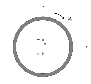
Figure 1: A binary system surrounded by a shell representing the rest of the universe.

III.1 Newton’s bucket and Mach’s principle

In Newton’s mechanics the rotation relative to the absolute space has physical consequences. Absolute rotation comes with a centrifugal effect which could be verified by means of a turning bucket filled with water. For Mach, instead, the parabolic shape of the water surface is just the manifestation of the rotation relative to the rest of the universe: “No one is competent to say how the experiment would turn out if the sides of the vessel increased in thickness and mass till they were ultimately several leagues thick” Mach ; i.e., nobody knows what would happen if the mass of the bucket were comparable to the rest of the universe or if the rest of the universe did not exist.

To study the issue in the light of equations (31), let us consider a binary star composed of two equal stars at a distance $2a$, orbiting its center of mass with circular motions of radius $a$. The rest of the universe will be represented by a spherical rigid shell centered at the center of mass of the system. The dynamics can be alternatively analyzed in the center-of-mass frame where the binary star is at rest but the shell rotates with angular velocity $\omega_{\circledcirc}$ (see Figure 1). In such a frame the centrifugal force that equilibrates the binary star comes from the rotation of the rest of the universe. Since the chosen frame is made up of the principal axes of inertia of the shell and the entire system, it results

$$\mathbf{J}=I_{\circledcirc}~{}\omega_{\circledcirc}~{}\mathbf{e}_{z}~{},\hskip 28.90755pt\mathbf{J}\cdot\mathbf{I}^{-1}=(\mathbf{I}^{-1})_{zz}~{}I_{\circledcirc}~{}\omega_{\circledcirc}~{}\mathbf{e}_{z}~{},$$ (40)

where $I_{\circledcirc}$ stands for the (isotropic) shell moment of inertia. The chosen frame is clearly non-Newtonian, since $\mathbf{J}\neq 0$. In Eq. (38) let be $k=1$ the label for one of the stars. Since $\mathbf{v}_{1}=0=\mathbf{P}/M$ and $\mathbf{I}^{-1}\cdot\mathbf{J}$ does not change in time, it results

$$~{}\mathbf{f}_{1}~{}-\mathbf{\nabla}_{1}V~{}=~{}0~{},~{}$$ (41)

where $-\mathbf{\nabla}_{1}V$ is the interaction force between the stars (the spherical shell does not produces gravity in the inner region). Equation (41) then says that the centrifugal force due to the rotating shell equilibrates the gravitational attraction. Since the inertia tensor $\mathbf{I}$ is diagonal in a frame of principal axes of inertia, then it is $(\mathbf{I}^{-1})_{zz}=1/I_{zz}$, where $I_{zz}=I_{\circledcirc}+2\,m\,a^{2}$. Thus the centrifugal force (37) is

$$|\,\mathbf{f}\,|~{}=~{}\frac{m~{}\omega_{\circledcirc}^{2}~{}a}{\left(1+\frac{2\,m\,a^{2}}{I_{\circledcirc}}\right)^{2}}~{}.$$ (42)

Since $I_{\circledcirc}>>m~{}a^{2}$, Eq. (41) approaches the form of the usual equation for orbital motion in Newton’s mechanics. However, if the rest of the universe were absent ($I_{\circledcirc}=0$) then the centrifugal force would vanish and the proposed orbital motion would make no sense, in agreement with Mach’s ideas.

The geometry inside a rotating shell has been studied in general relativity Brill ; Pfister . At the second order in the shell angular velocity, the inner geometry is flat for a conveniently prolate shell Pfister . This means that any rotating chart inside the shell will realize the usual inertial forces. However, this general relativity result lacks the significance of Eq. (42). In Eq. (42) the centrifugal force is caused by the rotation of the shell relative to the stars; its magnitude is proportional to the squared relative angular velocity. If the rotation or the shell evaporated then the centrifugal force would vanish and the binary star would collapse. In general relativity, instead, the evaporation of the shell has no consequences inside the shell: the geometry will continue to be flat, and the binary star will continue orbiting. Actually the general relativity solution possesses an inmaterial (“ethereal”) second “shell” at the infinity, where the boundary conditions for the metric are chosen.

III.2 Weak equivalence principle

The weak equivalence principle (WEP), one of the pillars of general relativity, lies in the core of Newtonian mechanics. The Newtonian motions of particles in an external gravitational potential do not depend on their masses, what means that the inertial-gravitational field can be locally canceled by changing to a freely falling frame. This is the basis for the geometrization of freely falling motions. Noticeably, we can hardly reproduce WEP in the context of Relational Mechanics. In fact, the inertial forces in Eq. (38) are not proportional to $m_{k}$, since $m_{k}$ is present in $\mathbf{P}/M$ and $\mathbf{I}^{-1}\cdot\mathbf{J}$. Then, given a self-gravitating system, we get that $m_{k}$ does take part in the equation for $\mathbf{r}_{k}(t)$ (even so, its contribution can be negligible for big systems, as seen in Eq. (41) where $m$ remains encapsuled in the ratio $2\,m\,a^{2}/I_{\circledcirc}$). Instead, in Newtonian mechanics the inertial forces are proportional to $m_{k}$ because the global properties of the isolated system, like $\mathbf{I}^{-1}\cdot\mathbf{J}$, have been substituted for absolute properties of the frame (absolute rotation, etc.). Actually, WEP is a statement concerning individual motions of particles. But the very idea of individual evolution means nothing in Relational Mechanics, since ${\bf r}_{k}(t)$ can be completely altered by a gauge transformation. In Relational Mechanics the observables (gauge invariant magnitudes) are the distances between particles. Instead, general relativity uses individual evolutions (world-lines) and space-time geometry as the basic concepts.

IV Elimination of the absolute time

So far, translations and rotations have been gauged. We have obtained the Lagrangian (20) which does not involve the idea of an absolute space: it can be used in any frame. However it still depends on the absolute time. To remove the absolute time we should gauge the time translation $t\longrightarrow t+\epsilon$. Since $t$ is a parameter identifying each configuration of the system in a temporal succession, a time translation is a relabeling (reparametrization) of the consecutive configurations. The invariance of the Lagrangian under rigid time translations is related to the conservation of the energy. Therefore, we expect that the requirement of gauge (local) invariance under reparametrizations will lead to a Hamiltonian first class constraint

$$\mathcal{H~{}}=~{}0~{},$$ (43)

i.e. some relation among the momenta that causes the vanishing of the Hamiltonian $H$.

Gauging the time translations does not involve counterterms for compensating the bad behavior of derivatives in the kinetic energy, since such behaviors do not come from the objects under differentiation but from the operator $d/dt$ itself. In fact, under local time translations $t\longrightarrow t+\epsilon(t)$ the derivative changes as

$$\frac{d}{dt}~{}\longrightarrow~{}\frac{1}{1+\dot{\epsilon}(t)}\ \frac{d}{dt}~{}\doteq~{}\frac{1}{N(t)}\ \frac{d}{dt}~{};$$ (44)

therefore velocities change as $\dot{q}\longrightarrow[1+\dot{\epsilon}(t)]^{-1}\,\dot{q}=N(t)^{-1}\,\dot{q}$. Since the invariance of the action is the invariance of $L\ dt$, then the behavior of the Lagrangian under reparametrizations should be

$$~{}L(q_{i},\,N^{-1}\ \dot{q}_{i})~{}=~{}N^{-1}\ L(q_{i},\,\dot{q}_{i})~{}.$$ (45)

This behavior characterizes the so called parametrized systems Lanczos ; Sundermeyer . The invariance of the action means that the action is unable to distinguish the trajectories $\mathbf{r}_{i}(t)$ from the reparametrized ones $\mathbf{r}_{i}(t+\epsilon(t))$; therefore, the parameter $t$ is physically irrelevant. Let us differentiate the equation (45) with respect to $N^{-1}$:

$$\sum\limits_{i}\ \dot{q}_{i}\ \frac{\partial L(q_{i},\,N^{-1}\ \dot{q}_{i})}{\partial(N^{-1}\ \dot{q}_{i})}~{}=~{}L(q_{i},\,\dot{q}_{i})~{}.$$ (46)

Since this result is valid whatever the function $N(t)$ is, one can substitute it with $N=1$ to conclude that parametrized systems come with a constraint $\mathcal{H}$ that cancels out the Hamiltonian, as expected. On the constraint surface, the Hamiltonian constraint $\mathcal{H}$ commutes with $\mathcal{P}_{\mu\,}$, $\mathcal{J}_{\nu}\,$ because $\mathcal{P}_{\mu\,}$, $\mathcal{J}_{\nu}$ are conserved quantities. Thus, the entire set of constraints remains first class. In a parametrized system, the evolution along the irrelevant time $t$ can be regarded as a gauge transformation, since the evolution is carried on by the first class Hamiltonian (see Eq. (28))

$$H^{\prime}=N(t)\ \mathcal{H}+\lambda^{\mu}(t)\ \mathcal{P}_{\mu}+\chi^{\nu}(t)\ \mathcal{J}_{\nu}~{}.$$ (47)

As explained in Section II.2, the freedom associated with $\mathcal{H}$ can be fixed by adding an admissible gauge condition $C$. So we choose $C=\tau(q,p)-t$, where $\tau(q,p)$ is invariant under translations and rotations, and satisfies $\{\tau,\mathcal{H}\}>0$. Thus it results $\dot{\tau}=\{\tau,H^{\prime}\}>0$, which means that $\tau(q,p)$ is a dynamical quantity that monotonically increases along the evolution; it is a physical clock defined by the system itself, also called internal time Kuchar ; Beluardi . The gauge condition $C=0$ means that the irrelevant parameter $t$ can be replaced by the internal time $\tau$.

IV.1 Hiding the time

A well known example of parametrized system is the relativistic free particle,

$$L\mathcal{~{}}=~{}-m\ \sqrt{\dot{Q}^{2}-\dot{q}^{2}}~{},$$ (48)

which displays a constraint between the conjugate momenta:

$$P=\frac{\partial L}{\partial\dot{Q}}=\frac{-m~{}\dot{Q}}{\sqrt{\dot{Q}^{2}-\dot{q}^{2}}}~{},\hskip 21.68121ptp=\frac{\partial L}{\partial\dot{q}}=\frac{m~{}\dot{q}}{\sqrt{\dot{Q}^{2}-\dot{q}^{2}}}~{}\hskip 21.68121pt\Longrightarrow\hskip 21.68121ptP=\pm\sqrt{p^{2}+m^{2}}.$$ (49)

The constraint surface splits into two sheets; we will keep the negative sign for $P$ ($\dot{Q}>0$). Then, the Hamiltonian constraint is

$$\mathcal{H~{}}=\mathcal{~{}}P+\sqrt{p^{2}+m^{2}}~{}=~{}0~{}.$$ (50)

This constraint causes the vanishing of the Hamiltonian $H$:

$$H\mathcal{~{}}=\mathcal{~{}}P~{}\dot{Q}+p~{}\dot{q}-L\mathcal{~{}}=~{}\frac{\sqrt{\dot{Q}^{2}-\dot{q}^{2}}}{m}\ (-P^{2}+p^{2}+m^{2})~{}=~{}0~{}.\mathcal{~{}}$$ (51)

We can fix the gauge by choosing the physical (internal) time $\tau=Q$ , that satisfies $\{\tau,\mathcal{H}\}=1$. However this is not the sole choice for the physical time. For instance, $\tau=Q\pm q$ yields $\{\tau,\mathcal{H}\}>0$; so, it is a good internal time. Any function $\tau=f(Q)$ such that $f^{\prime}(Q)>0$ is a good choice too. The gauge $Q-t=0$ fixes the irrelevant time parameter to be equal to $Q$. So $\dot{Q}=1$ and the Lagrangian becomes $L=-m\,\int\sqrt{1-{\dot{q}}^{2}}$. But, as said, there are many other forms for replacing the parameter $t$ with an internal time.

The free relativistic particle also shows how to parametrize a system: we achieve the property (45) by replacing the velocities $\mathbf{v}_{k}$ with $\mathbf{v}_{k}/\dot{Q}$ and multiplying the Lagrangian by a factor $\dot{Q}$. Finally, we take $Q$ to be a new canonical variable. For instance

$$L(\dot{q})\mathcal{~{}}=\mathcal{~{}}-m\sqrt{1-\dot{q}^{2}}~{}\longrightarrow~{}L(\dot{q},\dot{Q})\mathcal{~{}}=\mathcal{~{}}-m\ \dot{Q}\ \sqrt{1-\frac{\dot{q}^{2}}{\dot{Q}^{2}}}~{}=~{}-m\ \sqrt{\dot{Q}^{2}-\dot{q}^{2}}~{}.$$ (52)

So, a possible strategy for eliminating the absolute time consists in adding the system with a new canonical variable $Q$ causing the parameter $t$ becomes physically irrelevant. The new variable does not imply a new degree of freedom, since it comes together with a new constraint (the Hamiltonian constraint); so the original number of degrees of freedom of the non-parametrized system is kept. Once the variable $Q$ was introduced through this procedure, it can be mixed with the rest of canonical variables by means of canonical transformations. It could be said that the procedure hides the absolute time among the canonical variables. However, once the time was hidden, there are many internal times –all of them on an equal footing– that can be retrieved by fixing the gauge. Thus, the privileged absolute time was lost forever.

Let us parametrize a classical particle:

$$L(\mathbf{r},\mathbf{v},\dot{Q})~{}=\frac{1}{\dot{Q}}~{}\frac{m\ \mathbf{v}^{2}}{2\,}~{}-~{}\dot{Q}\ V~{}.$$ (53)

The canonical momenta are

$$\mathbf{p}\ =\ \frac{m\,\mathbf{v}}{\dot{Q}}~{},\hskip 21.68121ptP\ =\ -\frac{m\ \mathbf{v}^{2}}{2\ \dot{Q}^{2}}-V=-\frac{\mathbf{p}^{2}}{2\,m}-V~{}.$$ (54)

Then the Hamiltonian constraint is

$$\mathcal{H~{}}=\mathcal{~{}}P+\frac{\,\mathbf{p}^{2}}{2\,m}+V~{}=~{}0~{},$$ (55)

and the Hamiltonian $H=P~{}\dot{Q}+\mathbf{p}\cdot\mathbf{v}-L$ vanishes. The Hamiltonian evolution is governed by $H^{\prime}=N(t)\,\mathcal{H}$. Then it is

$$\mathbf{\dot{r}}\ =\ N(t)\,\{\mathbf{r},\mathcal{H}\}\ =\ N(t)\,\frac{\mathbf{p}}{m}~{},\hskip 21.68121pt\hskip 21.68121pt\mathbf{\dot{p}}\ =\ N(t)\,\{\mathbf{p},\mathcal{H}\}\ =\ -N(t)\,\mathbf{\nabla}V~{},$$ (56)

whose solution is expressed in terms of an arbitrary time parameter $\int N(t)\,dt$ that can be freely fixed. Besides it is

$$\dot{Q}\ =\ N(t)\,\{Q,\mathcal{H}\}\ =\ N(t)~{},\hskip 21.68121pt\hskip 21.68121pt\dot{P}\ =\ N(t)\,\{P,\mathcal{H}\}\ =\ 0~{}.$$ (57)

Equation (54) shows that the conserved quantity $P$ is (minus) the energy of the classical particle. Equation (57) shows that $Q$ is a pure gauge variable: its dynamics remains ambiguous since $N(t)$ is arbitrary. Like in the previous example, one could fix the gauge by choosing $\dot{Q}=1$, or any other admissible gauge condition.

The procedure described in this subsection can be used to parametrize the Lagrangian (20). In such case, the so built parametrized Lagrangian will have $3N+1$ canonical variables, since $Q$ is added to the $N$ vectors $\mathbf{r}_{k}$, together with $7$ first class constraints. The number of degrees of freedom will then result $3N-6$. In this sense, any system displaying an absolute time, like the one described by Lagrangian(20), could be regarded as a gauge-fixed parametrized system.

IV.2 Jacobi action

A different approach to the problem of eliminating the absolute time consists in regarding the clock as a piece of the original mechanical system. In such case, we will not add a canonical variable $Q$ to the system of $N$ particles. Instead, we will try to relate the evolution of the rest of the system to that piece of the system playing the role of clock. If convenient, a parameter $t$ will be still introduced; but the action cannot be sensitive to it. The action should contain only positions and velocities of the particles and, at the same time, behave as a parametrized system. These features are fulfilled by the Jacobi-like action Lanczos whose Lagrangian is Barbour75 ; Barbour77 ; Barbour82

$$L~{}=~{}2\,\sqrt{\Lambda-V}\,\sqrt{T}~{},$$ (58)

where $\Lambda$ is a constant and $T$ is the compensated kinetic energy of Lagrangian (20). In fact, $T$ is made up of terms quadratic in the velocities; then, $\sqrt{T}\ dt$ is invariant under reparametrizations. In this case the canonical momenta are

$$\mathbf{p}_{k}\ =\ \frac{\sqrt{\Lambda-V}}{\sqrt{T}}\ \frac{\partial T}{\partial\mathbf{v}_{k}}~{},$$ (59)

where $\partial T/\partial\mathbf{v}_{k}$ are the momenta obtained in Eq. (22); they satisfy (see Eq. (21))

$$\sum_{k}\frac{1}{2\,m_{k}}\ \frac{\partial T}{\partial\mathbf{v}_{k}}\cdot\frac{\partial T}{\partial\mathbf{v}_{k}}\ =\ T~{}.$$ (60)

Therefore we obtain the Hamiltonian constraint

$$\mathcal{H}\ =\ \sum_{k}\,\frac{\mathbf{p}_{k}\cdot\mathbf{p}_{k}}{2\ m_{k}}+V-\Lambda\ =\ 0~{}.$$ (61)

Thus $\Lambda$ looks as the total energy of the universe. However, differing from Jacobi’s idea, its value cannot be chosen within the initial conditions because $\Lambda$ enters the action as a universal constant. Furthermore, the initial conditions are constrained to fulfill the Eq. (61) for a given value of $\Lambda$. Instead, the constraint (55) allowed the total energy to take any value because the initial value of $P$ was not constrained. This is the only difference between both approaches. So this approach displays one degree of freedom less than the former: since the number of variables has not been increased, the number of degrees of freedom reduces to $3N-7$. Otherwise the dynamics is still governed by the equations (56), because the form of $\mathcal{H}$ as a function of $\mathbf{r}_{k}$, $\mathbf{p}_{k}$ is the same in both cases. It can be verified that Lagrange equations recover their usual form too, since the constraint implies that the factor $\sqrt{\Lambda-V}/\sqrt{T}$ is equal to $1$. Concerning the choice of an internal time $\tau(\mathbf{r}_{k},\mathbf{p}_{k})$, see Footnote 8.

V Scale invariance

In recent years much attention has been focused on shape-dynamics Barbour03 ; Mercati ; Anderson , which is a kind of relational mechanics with a local scale invariance. The scale transformation is

$$\mathbf{r}_{i}~{}\longrightarrow(1+\lambda)~{}\mathbf{r}_{i}~{}.$$ (62)

This transformation is generated by

$$\mathcal{G}\doteq\sum\limits_{k}~{}\mathbf{p}_{k}\cdot\mathbf{r}_{k}~{},$$ (63)

since $\delta\mathbf{r}_{i}=\lambda\{\mathbf{r}_{i~{}},\mathcal{G}\}$. In Ref. Barbour03, $\mathcal{G}$ is called the dilatational momentum. Scale transformation should not be confused with a change of units. A change of units not only scales positions and velocities but also changes the fundamental constants entering the Lagrangian, in such a way that the Lagrangian is affected only by a global harmless factor. Instead, a (rigid) scaling only affects positions and velocities; so one cannot expect an inoffensive effect. In general, Lagrangians are not invariant under rigid scalings. However, let us consider the parametrized Lagrangian (58) in the case $\Lambda=0$. This Lagrangian would be invariant under rigid scalings if the interaction potentials were inversely proportional to the squared distances. In fact, under rigid scalings the compensated kinetic energy transforms as

$$T~{}\longrightarrow(1+\lambda)^{2}~{}T$$ (64)

($\mathbf{v}_{k}\rightarrow(1+\lambda)\,\mathbf{v}_{k\ }$; $\mathbf{J}\cdot\mathbf{I}^{-1}\cdot\mathbf{J}$ is homogeneous of degree $2$ in the velocities but homogeneous of degree $0$ in the positions). So the behavior of $T$ under rigid scalings is compensated by the potential only if $V_{ij}=\kappa/r_{ij}^{2}$. We will now consider the gauging of the scale invariance. Since $\mathcal{G}$ is going to be the generator of a gauge transformation, we expect the constraint

$$\mathcal{G}=0.$$ (65)

Concerning $\mathcal{P}_{\mu\,}$ and $\mathcal{J}_{\nu}$, $\mathcal{G}$ is a first class constraint; in fact, $\mathcal{G}$ is invariant under rotations and $\{\mathcal{G},\mathcal{P}_{\mu\,}\}=\mathcal{P}_{\mu\,}$. Besides $\{\mathcal{G},\mathcal{H}\}$ vanishes on the constraint surface in the considered case. In fact

$$\{\mathcal{G},\mathcal{H}\}~{}=~{}\{\sum\limits_{k}\,\mathbf{p}_{k}\cdot\mathbf{r}_{k}~{},\sum\limits_{i}\,\frac{\mathbf{p}_{i}\cdot\mathbf{p}_{i}}{2~{}m_{i}}+V\}~{}=~{}\sum\limits_{k}\,\left(\frac{\mathbf{p}_{k}\cdot\mathbf{p}_{k}}{m_{k}}-\mathbf{r}_{k}\cdot\mathbf{\nabla}_{k}V\right)~{}=~{}2\ (\mathcal{H}-V)-\sum\limits_{k}\,\mathbf{r}_{k}\cdot\mathbf{\nabla}_{k}V~{},$$ (66)

where

$$\sum\limits_{k}\,\mathbf{r}_{k}\cdot\mathbf{\nabla}_{k}V~{} = ~{}\sum\limits_{k}\sum\limits_{i<j}\,\mathbf{r}_{k}\cdot\mathbf{\nabla}_{k}V_{ij}(r_{ij})~{}=~{}\frac{1}{2}\sum\limits_{k}\sum\limits_{i\neq j}\,\frac{\partial V_{ij}}{\partial r_{ij}}~{}\mathbf{r}_{k}\cdot\mathbf{\nabla}_{k}r_{ij}$$ (67)

$$= ~{}\frac{1}{2}\left(\sum\limits_{k\neq j}\,\frac{\partial V_{kj}}{\partial r_{kj}}~{}\frac{\mathbf{r}_{k}\cdot\mathbf{r}_{kj}}{r_{kj}}~{}\mathbf{-}\sum\limits_{k\neq i}\,\frac{\partial V_{ik}}{\partial r_{ik}}~{}\frac{\mathbf{r}_{k}\cdot\mathbf{r}_{ik}}{r_{ik}}\right)~{}=~{}\frac{1}{2}\sum\limits_{k\neq j}\,\frac{\partial V_{kj}}{\partial r_{kj}}~{}\frac{\mathbf{r}_{kj}\cdot\mathbf{r}_{kj}}{r_{kj}}~{}=~{}\sum\limits_{k<j}\,\frac{\partial V_{kj}}{\partial r_{kj}}~{}r_{kj}~{}.$$

Since $V_{kj}\propto r_{kj}^{-2}$ one obtains

$$\sum\limits_{k}\,\mathbf{r}_{k}\cdot\mathbf{\nabla}_{k}V~{}=~{}-2~{}V.$$ (68)

Thus one gets the vanishing of $\{\mathcal{G},\mathcal{H}\}$ on the constraint surface:

$$\{\mathcal{G},\mathcal{H}\}~{}=~{}2\ \mathcal{H}\,~{}.$$ (69)

Let us study the compensating term we should add to the Lagrangian (20) for gauging the scale invariance. Since velocities change as

$$\mathbf{v}_{k}~{}\longrightarrow(1+\lambda)~{}\mathbf{v}_{k}\,+\,\dot{\lambda}~{}\mathbf{r}_{k}~{},$$ (70)

the infinitesimal change of the intrinsic kinetic energy is

$$\sum\limits_{i<j}\,\frac{m_{i}~{}m_{j}}{M}~{}\mathbf{v}_{ij}\cdot\delta\mathbf{v}_{ij}~{}=~{}\lambda\,\sum\limits_{i<j}\,\frac{m_{i}~{}m_{j}}{M}~{}\mathbf{v}_{ij}\cdot\mathbf{v}_{ij}\,+\,\dot{\lambda}\sum\limits_{i<j}\,\frac{m_{i}~{}m_{j}}{M}~{}\mathbf{v}_{ij}\cdot\mathbf{r}_{ij}~{}.$$ (71)

This behavior can be compensated by the term $I^{-1}G^{2}/2$ , where $G$ is the intrinsic virial (the virial in a center-of-mass frame):

$$G~{}\doteq~{}\sum\limits_{i<j}\,\frac{m_{i}~{}m_{j}}{M}~{}\mathbf{v}_{ij}\cdot\mathbf{r}_{ij}~{}=~{}\sum\limits_{k}\,m_{k}~{}\mathbf{v}_{k}\cdot\mathbf{r}_{k}\,-\,\mathbf{P}\cdot\mathbf{R}~{}=~{}\sum\limits_{k}\,m_{k}~{}\mathbf{v}_{k}\cdot(\mathbf{r}_{k}-\mathbf{R)~{}},$$ (72)

and $I$ is the intrinsic scalar moment of inertia:

$$I~{}\doteq~{}\sum\limits_{i<j}\,\frac{m_{i}~{}m_{j}}{M}~{}r_{ij}^{2}~{}~{}=~{}\sum\limits_{k}\,m_{k}~{}r_{k}^{2}\,-\,MR^{2}~{}~{}=~{}\sum\limits_{k}\,m_{k}~{}|\mathbf{r}_{k}-\mathbf{R}|^{2}~{}.$$ (73)

Both $G$ and $I$ are invariant under local rotations and translations; so, they do not interfere the local invariance of the kinetic energy. In $I^{-1}G^{2}$ only the behaviors of the velocities are relevant under scaling, because the scaling factors coming from the $\mathbf{r}_{ij}$’s compensate each other. Therefore

$$\delta\left(I^{-1}G^{2}/2\right)~{}=~{}I^{-1}G~{}\delta G~{}=~{}I^{-1}G~{}\sum\limits_{i<j}\,\frac{m_{i}~{}m_{j}}{M}~{}(\lambda~{}\mathbf{v}_{ij}+\dot{\lambda}~{}\mathbf{r}_{ij}~{})\cdot\mathbf{r}_{ij}~{}=~{}\lambda~{}I^{-1}G^{2}\,+\,\dot{\lambda}~{}G$$ (74)

Besides the term $-(1/2)~{}\mathbf{J}\cdot\mathbf{I}^{-1}\cdot\mathbf{J}$ in (20) changes because the velocities change (the scaling factors coming from $\mathbf{r}_{ij}$’s compensate each other). So, we just consider the change

$$\delta\mathbf{J~{}}=~{}\sum\limits_{i<j}\,\frac{m_{i}~{}m_{j}}{M}~{}\mathbf{r}_{ij}\times(\lambda~{}\mathbf{v}_{ij}+\dot{\lambda}~{}\mathbf{r}_{ij}~{})~{}=~{}\lambda~{}\mathbf{J~{},}$$ (75)

which coincides with a rigid change; so it does not need a compensating term. Thus the kinetic energy

$$T~{}~{}=~{}\sum\limits_{i<j}\,\frac{m_{i}~{}m_{j}}{2M}~{}\mathbf{v}_{ij}\cdot\mathbf{v}_{ij}~{}-\,\frac{1}{2}~{}\mathbf{J}\cdot\mathbf{I}^{-1}\cdot\mathbf{J}\,-\,\frac{1}{2}~{}I^{-1}~{}G^{2}~{}$$ (76)

behaves under local scalings just as under rigid scalings. The conjugated momenta

$$\mathbf{p}_{k}\ =\ m_{k}\left[\mathbf{v}_{k}-\frac{\mathbf{P}}{M}-(\mathbf{I}^{-1}\cdot\mathbf{J})\times(\mathbf{r}_{k}-\mathbf{R})-I^{-1}~{}G~{}(\mathbf{r}_{k}-\mathbf{R})\right]~{}$$ (77)

satisfy, as expected, the constraint (65). Moreover, the new compensating term $I^{-1}~{}G~{}(\mathbf{r}_{k}-\mathbf{R})$ does not modify the constraints (23). The momenta (77) contain the particle velocities relative to a frame based at the center of mass that rotates with the mean angular velocity of the system, diminished by a sort of mean radial velocity of the system. Therefore, the global expansion has been deducted from the particle velocities. As a consequence, the momenta have the same behavior under rigid and local scalings, namely $\delta\mathbf{p}_{k}=~{}\lambda\mathbf{\ \{p}_{k\,},\mathcal{G}\}$. Kinetic energy (76) can be rewritten as

$$T~{}~{}=~{}\sum\limits_{k}\,\frac{m_{k}}{2}~{}\left|\mathbf{v}_{k}-\frac{\mathbf{P}}{M}-(\mathbf{I}^{-1}\cdot\mathbf{J})\times(\mathbf{r}_{k}-\mathbf{R})-I^{-1}~{}G~{}(\mathbf{r}_{k}-\mathbf{R})\right|^{2}~{}.$$ (78)

The system has $3N$ canonical coordinates and $8$ first class constraints $\mathcal{P_{\mu\,}}$,$~{}\mathcal{J_{\nu\,}}$, $\mathcal{G}$, $\mathcal{H}$. So, $3N-8$ genuine degrees of freedom are left in shape-dynamics. For instance, $3$ particles would have $2$ degrees of freedom in shape-dynamics, that relate to the two angles one needs to define a triangle regardless of its size and orientation; but one of these degrees of freedom is related to the internal time.

VI Conclusions

Newton’s mechanics relies on external symmetries linked to the concepts of absolute space and time. These symmetries manifest themselves through the idea of inertial frames together with the Galilean group as a tool for relating coordinates belonging to different inertial frames. Instead, Relational Mechanics describes the system by means of equations that can be used in any frame. This means that Relational Mechanics is not involved with absolute magnitudes but only with the relative motions of the particles of the system. This goal is reached by gauging the Galilean group; i.e., by adding compensating terms that makes the kinetic energy behave in the same way under rigid and local translations and rotations. The compensating terms do not contain external fields but are built with the own variables of the system, in such a way that the gauge invariant Lagrangian results to be written just in terms of intrinsic quantities (notice that intrinsic quantities (10), (15) and (19) look like the respective usual quantities in a center-of-mass frame). As in any gauge theory, the generators of gauge transformations –3 translations and 3 rotations in this case– become first class constraints. So, the system loses 6 degrees of freedom since global time-dependent translations and rotations have been excluded from the category of motions: they do not constitute changes of the relations between particles. In the Lagrange formulation of Relational Mechanics, two sets of initial conditions that differ in a gauge transformation (a change to an arbitrarily moving frame) are equivalent; in particular, any configuration corresponding to a rigid motion is equivalent to the state of rest. In the Hamiltonian formulation, the losing of 6 degrees of freedom is evidenced in the fact that the set of initial data for the canonical variables is constrained by 6 constraint functions.

Differing from the absolute space, absolute time is not eliminated by means of counterterms that covariantize the time derivative. The gauging of time translations affects the operator $d/dt$ itself. So, we have to resort to forms of Lagrangian that reproduce the usual dynamics but leave the parameter $t$ as an irrelevant quantity that can be arbitrarily changed; these are the parametrized Lagrangians. In particular, the Jacobi action describes a parametrized system which acquires scale invariance if the potentials are inversely proportional to the squared distances. This rigid invariance can be gauged by introducing a new counterterm in the kinetic energy. The result is the Lagrangian for the so called shape-dynamics.

Relational equations of motion (31) exhibit two types of interaction. On the one hand, the potential $V$ provides gauge invariant forces between pairs of particles. On the other hand, each particle interacts with the entire universe through gauge dependent inertial forces. The unquestionable success of Newton’s laws can be fully understood in the framework of Relational Mechanics: Newton’s laws are valid in any frame where the center of mass of the universe moves at a constant velocity, and the total intrinsic angular momentum of the universe $\mathbf{J}$ vanishes (however, Newtonian solutions must be filtered by the gauge condition $\mathbf{J}=0$). This result realizes Mach’s principle, in the sense that these privileged Newtonian frames are selected by the distribution of matter in the universe. The origin of the inertial forces lies in the entire universe, as seen in the example of Newton’s bucket.

In his famous article of 1916, Einstein began §2 by saying “In classical mechanics, and no less in the special theory of relativity, there is an inherent epistemological defect which was, perhaps for the first time, clearly pointed out by Ernst Mach” Einstein16 . He then paraphrased Newton’s thought experiment of the rotating bucket by proposing two equally constituted fluid bodies in relative rotation around the axis joining their centers, at a relative distance enough large to ignore the gravitational interaction. Einstein said that if one of the bodies resulted to be spherical and the other one an ellipsoid of revolution, then it should exist a physical reason other than the rotation with respect to the absolute space for such a difference. Relational Mechanics can tackle the issue because no difference is expected if the bodies are the sole constituents of the universe. Instead, the rotation relative to the rest of the universe will produce the equatorial deformation.

- (1) H.G. Alexander (ed.), The Leibniz-Clarke Correspondence Together with Extracts from Newton’s Principia and Opticks (Manchester University Press: Manchester, 1956).
- (2) E. Mach, Die Mechanik in ihrer Entwicklung. Historisch-kritisch dargestellt (F.A. Brockhaus: Leipzig, 1883) (The Science of Mechanics: A Critical and Historical Account of Its Development (The Open Court Publishing Co.: Chicago, 1893)).
- (3) A. Einstein, The Meaning of Relativity (Princeton University Press: Princeton, 1922).
- (4) H. Reissner, Phys. Z. 15 (1914), 371-375 (English translation in Ref. Barbour95, ).
- (5) E. Schrödinger, Annalen der Physik 382 (1925), 325-336 (English translation in Ref. Barbour95, ).
- (6) J.B. Barbour, Nuovo Cimento B 26 (1975), 16-22.
- (7) J.B. Barbour and B. Bertotti, Nuovo Cimento B 38 (1977), 1-27.
- (8) J.B. Barbour and H. Pfister (eds.), Einstein Studies, vol. 6: Mach’s Principle: From Newton’s Bucket to Quantum Gravity (Birkhäuser: Boston, 1995).
- (9) J.B. Barbour and B. Bertotti, Proc. R. Soc. Lond. A 382 (1982), 295-306.
- (10) J. Barbour, Class. Quantum Grav. 20 (2003), 1543-1570.
- (11) S. Gryb, Phys. Rev. D 80 (2009), 024018.
- (12) J. Ehlers, in The Physicist’s Conception of Nature, ed. by J. Mehra (Reidel: Dordrecht, 1973).
- (13) D. Lynden-Bell, in B. Warner (ed.), Variable Stars and Galaxies (in honour of M.W. Feast), ASP Conference Series 30 (1992).
- (14) D. Lynden-Bell, in J.B. Barbour and H. Pfister (eds.), Einstein Studies, vol. 6: Mach’s Principle: From Newton’s Bucket to Quantum Gravity (Birkhäuser: Boston, 1995).
- (15) D. Lynden-Bell and J. Katz, Phys. Rev. D 52 (1995), 7322-7324.
- (16) P.A.M. Dirac, Lectures on Quantum Mechanics, Belfer Graduate School of Science (Yeshiva University: New York, 1964).
- (17) M. Henneaux and C. Teitelboim, Quantization of gauge systems (Princeton University Press: Princeton, 1992).
- (18) M. Friedman, Foundations of Space-Time Theories: Relativistic Physics and Philosophy of Science (Princeton University Press: Princeton, 1983).
- (19) D. Brill and J.M. Cohen, Phys. Rev. 143 (1966), 1011-1015.
- (20) H. Pfister and K.H. Braun, Class. Quantum Grav. 2 (1985), 909-918.
- (21) C. Lanczos, The Variational Principles of Mechanics (Dover Publications: New York, 1986).
- (22) K. Sundermeyer, Constrained Dynamics, Lectures Notes in Physics 169 (Springer-Verlag: Berlin, 1982).
- (23) K.V. Kuchař, in Proceedings of the 4th. Canadian Conference on General Relativity & Relativistic Astrophysics, eds. G. Kunstatter, D. Vincent and J. Williams (World Scientific: Singapore, 1992).
- (24) S.C. Beluardi and R. Ferraro, Phys.Rev. D 52 (1995), 1963-1969.
- (25) F. Mercati, A Shape Dynamics Tutorial, arXiv:1409.0105 (2014).
- (26) E. Anderson, The problem of time and quantum cosmology in the relational particle mechanics arena, arXiv:1111.1472v3 (2011).
- (27) A. Einstein, Annalen der Physik 354 (1916), 769-822 (English translation in H.A. Lorentz, A. Einstein, H. Minkowski and H. Weyl, The Principle of Relativity: A Collection of Original Memoirs on the Special and General Theory of Relativity (Dover Publications: New York, 1952) ).
- (28) J. Barbour, T. Koslowski and F. Mercati, Class. Quantum Grav. 31 (2014), 155001.