Partial long-range order in antiferromagnetic Potts models

Abstract

The Potts model plays an essential role in classical statistical mechanics, illustrating many fundamental phenomena. One example is the existence of partially long-range-ordered states, in which some degrees of freedom remain disordered. This situation may arise from frustration of the interactions, but also from an irregular but unfrustrated lattice structure. We study partial long-range order in a range of antiferromagnetic $q$-state Potts models on different two-dimensional lattices and for all relevant values of $q$. We exploit the power of tensor-based numerical methods to evaluate the partition function of these models and hence to extract the key thermodynamic properties – entropy, specific heat, magnetization, and susceptibility – giving deep insight into the phase transitions and ordered states of each system. Our calculations reveal a range of phenomena related to partial ordering, including different types of entropy-driven phase transition, the role of lattice irregularity, very large values of the critical $q_{c}$, and double phase transitions.

I Introduction

The Potts model Wu1982_RMP54-235 is a cornerstone of classical statistical physics. First appearing in Potts’ Ph.D. thesis Potts_PHD_thesis as a generalization of the Ising model, it is a simple but highly nontrivial model. Indeed, the family of $q$-state antiferromagnetic (AF) Potts models displays a rich and complex range of behavior, providing many examples of different phase transitions, critical phenomena, ordered states, and universality classes. Although the $q=2$ Potts model is equivalent to the Ising model, and thus has exact solutions for all planar lattices with nearest-neighbor interactions domb_green , including the square square_exact , triangular trian_honey_exact , and honeycomb trian_honey_exact geometries, exact results for $q>2$ are rare. Many other problems in statistical mechanics are closely related to the Potts model, including vertex models Baxter_vertex , bond and vertex coloring problems Baxter_coloring , and loop models Jacobsen_loop .

The behavior of the AF Potts model is dictated by the interplay between $q$, the number of states per site, and the lattice geometry. When $q$ is small compared to the average coordination number ${\bar{z}}$ of the lattice, at low temperatures the limited number of degrees of freedom will in general be fixed, and ordered, by geometrical and interaction requirements. However, when $q$ is similar to or greater than ${\bar{z}}$, the entropy is such that the system may not order at any temperature Salas1997_JSP86-551 . In addition to the conventional zero-temperature limits of complete order or disorder, AF Potts models show two further possibilities. One is that the ground state is genuinely critical, the result of an arrested “zero-temperature phase transition” to an ordered state; this type of physics is known in the $q=3$ AF Potts model on the square Salas1998_JSP92-729 and kagome kagome_qc lattices and in the $q=4$ AF Potts model on the triangular lattice triangular_qc . The other is that some, but not all, of the degrees of freedom of the system may form a state of partial long-range order x ; Kotecky2008_PRL101-030601 ; partial or complete ordering processes occur at different types of “finite-temperature phase transition.”

At a conventional phase transition, the order parameter becomes finite everywhere in the system to minimize the free energy, and the result is a state of complete order at zero temperature. In the example of the ferromagnetic Ising model, all spins are oriented either upwards or downwards in the ground state. However, in systems with sufficiently many degrees of freedom (sufficiently large entropy, as in a Potts model with sufficiently high $q$), the crossover to a ground state optimizing the resulting entropic contribution may occur in a step-wise fashion. The minimization of energy may be achieved in many different ways, and may involve only some of the lattice sites. The remaining degeneracy, and the type of order, is then determined by the maximization of entropy. The result is an “entropy-driven” transition, usually occurring at a finite temperature, and to a state of partial order. On cooling to zero temperature, if the system retains a nonzero “residual” entropy then a ground state with order on only a subset of the lattice sites can be achieved. The best-known example of the physics of extensive ground-state degeneracy is found in ice Pauling .

The majority of prior work on partial order has concerned frustrated systems, where the energy cannot be minimized locally, meaning for all bonds simultaneously Lipowski . The AF Ising model on the triangular lattice trian_honey_exact is an archetypal frustrated system, because no spin configuration can minimize all three bonds on a triangle simultaneously. Frustrated systems share the same property of highly degenerate ground states, arising from their frustrated interactions, and the formation of partially ordered states offers one avenue for partial frustration relief and partial entropy reduction.

When partial order arises in unfrustrated systems x , its origin lies only in configurational entropy effects. In 2008, Kotecky and coauthors Kotecky2008_PRL101-030601 found partial long-range order in the $q=3$ AF Potts model on the diced lattice, performing both analytical and numerical studies of the accompanying finite-temperature phase transition. In 2011, we Chen2011_Phys.Rev.Lett.107-165701 traced their result to the extensive zero-temperature entropy (residual entropy per site) of this lattice, which arises because it is “irregular” in the sense of having differently coordinated sites (we defer a discussion of lattice types to Sec. II). From this insight we demonstrated the existence of finite-temperature phase transitions and partial order in the $q=4$ Potts models on the Union-Jack and centered diced lattices. Partial order is the result of a partial symmetry-breaking, and we found that, depending on the Potts model in question, the singularity associated with this breaking of symmetry may be either almost as strong as a full symmetry-breaking, or may be remarkably weak and difficult to detect.

Partial order in the ground state is known exactly in a number of models. In the spin-$S$ AF Ising model on the triangular lattice, for sufficiently large $S$ the ground state is partially ordered on two of the hexagonal sublattices but disordered on the third Nagai1993_PRB47-202 . Also in two dimensions, the ground states of the AF Ising model on the Union-Jack lattice Vaks1966_JETPLetters22-820 , kagome lattice Azaria1987_PRL59-1629–1632 , dilute centered square lattice Debauche1992_PRB46-8214–8218 , anisotropic triangular lattice Diep1991_Phys.Rev.B43-8759–8762 , and Villain lattice (anisotropic square lattice) Villan are all partially ordered. Partial order also exists for some frustrated systems, such as the $q=3$ Potts model on the Villain lattice Foster2001_JPA34-5183 ; Foster2004_PRB70-014411 . Three-dimensional classical models with partial order are mostly frustrated, including the Ising model on the accumulated triangular Blankschtein1984_PRB29-5250–5252 and body-centered cubic (BCC) Azaria1989_EPL9-755 lattices, the classical Heisenberg model on the BCC lattice Santamaria1997_JAP81-5276-5278 , models on the simple cubic lattice Blankschtein1984_PRB30-1362–1365 ; Diep1985_JPC18-1067 , the $q=4$ AF Potts model on the diamond lattice Igarashi2010_JPCS200-022019 and the XY model on the checkerboard lattice Boubcheur1998_PRB58-400–408 . Experimentally, partial order has been observed in the frustrated AF material Gd₂Ti₂O₇ Stewart2004_JPCM16-L321 . Partial order is also predicted for the periodic Anderson model on the triangular lattice Hayami2011_JPSJ80-073704 ; Hayami2011_ArXive-prints-1107.4401 and the Heisenberg model on the BCC lattice Quartu1997_PRB55-2975–2980 ; Santamaria1998_JAP84-1953-1957 .

Although the Potts model is one of the simplest in statistical physics, its analytical study has been restricted by the limited number of exactly known results beyond $q=2$. Methods including height mapping Kotecky2008_PRL101-030601 have some general utility, while mappings to related coloring problems Baxter_coloring are useful in specific cases. Previous numerical studies of Potts models have made use of Monte Carlo WSK_1 ; WSK_2 and transfer-matrix Trans_Mat_1 ; Trans_Mat_2 techniques. Monte Carlo simulations are accurate, and can study large but finite lattice sizes, while transfer-matrix methods are infinite in one spatial dimension but finite in the other(s), and can be used to study fractional values of $q$.

In this paper we introduce (Sec. III) a set of tensor-based numerical methods, which are quite generally applicable in classical statistical mechanics. The partition function is written as the trace over a network of tensors representing the states of the system on an infinite lattice, and in its evaluation the truncation is performed systematically in the tensor dimension. Because it evaluates the partition function, this calculational approach gives access in principle to all thermodynamic quantities, and is not very resource-intensive in comparison with other numerical techniques.

We apply the tensor-network approach to perform a detailed analysis of partial order in AF Potts models qiaoni_thesis . We consider a number of irregular lattices in two dimensions, and calculate thermodynamic quantities including the entropy, specific heat, magnetization, and magnetic susceptibility. We use these qualitatively to investigate the partial order or partial breaking of symmetry, which is shown by all the models, and quantitatively to characterize the phase transitions and partially ordered states. We find lower bounds for the critical values of $q$ on each lattice and illustrate the phenomenon of double phase transitions in particular models. Our results show the power of tensor-based numerical methods for gaining fresh insight into long-standing problems in classical statistical mechanics.

The structure of this paper is as follows. In Sec. II we review the Potts model, the classes of lattice we consider in two dimensions, and some known results concerning $q$, regular geometries, and phase transitions. Section III describes in detail the tensor-based numerical techniques we employ to compute the partition function and thermodynamics of each model. In Sec. IV we focus on the entropy-driven phase transition, using the entropy and specific heat to compare and contrast its form on a number of Laves lattices. We calculate in Sec. V the magnetization of the models studied in Sec. IV, in order to characterize the partial order through its order parameter and susceptibility. In Sec. VI we expand our discussion to models showing two successive phase transitions with an intermediate state of partial order occurring for entropic reasons. For completeness, in Sec. VII we examine Potts models on two lattices, which have a high ground-state degeneracy and do display partial order, but where the entropy is sub-extensive, i.e. the residual entropy per site is $0$. Section VIII contains a brief summary and conclusion.

II Models

II.1 Potts Model

In a $q$-state Potts model, the local variable at site $i$ may take one of $q$ different states, which we label as $\sigma_{i}=0,1,\dots\;q-1$. The Hamiltonian

$${\cal H}=J\sum_{<i,j>}\delta_{\sigma_{i}\sigma_{j}}-H\sum\limits_{i\in\cal{L}}\delta_{\sigma_{i},0}$$ (1)

consists of two terms, one for interactions between nearest-neighbor local variables for every bond of the lattice, and one for an external field $H$ coupled to one of the $q$ states and for one sublattice $\cal{L}$. In the ferromagnetic Potts model, $J<0$, a negative energy contribution is obtained if the neighboring sites are in the same state, while in the AF case, $J>0$, neighboring sites tend to occupy different states.

In the case $J<0$, long-range order is favored and the ground state always has ferromagnetic order. It has been proven in two dimensions that the finite-temperature phase transition to a disordered state is continuous if $q\leq 4$ and is first-order if $q>4$ Baxter_q_4_order . Although there is no exact solution in three dimensions, numerical results 3D_ferr_Potts ; rwxcnx indicate that a first-order phase transition occurs for $q\geq 3$.

The AF case is far richer and more complex. If the different local states are denoted by different colors, at zero temperature the neighboring sites should not have the same color. Thus the AF Potts model at $T=0$ is equivalent to a vertex coloring problem. By using the Dobrushin Uniqueness Theorem Dobrushin1968_Theor.Prob.Appl.13-197-224 ; Dobrushin1970_Theor.Prob.Appl.15-458-486 , Salas and Sokal Salas1997_JSP86-551 proved that for sufficiently large $q$ the correlation function exhibits exponential decay at all temperatures, including $T=0$. The model is therefore disordered even in the ground state, and no phase transition occurs. For small $q$, by contrast, an ordered (or, from above, partially ordered) ground state is likely. Based on this insight, it is thought that for every lattice there exists a value $q_{c}$ for which the system is disordered at all temperatures if $q>q_{c}$. For $q=q_{c}$ the system is critical at zero temperature, a situation we discuss below. Any behavior is possible if $q<q_{c}$, and typically one expects a phase transition of first or second order to a type of long-range-ordered state Salas1998_JSP92-729 .

Table 1: Values $q_{c}$ at which the $q$-state AF Potts model is critical at zero temperature for different two-dimensional lattices. For regular lattices, ${\bar{z}}$ denotes the coordination number, while it represents the average coordination for irregular lattices. For the square, kagome, and triangular lattices, the value of $q_{c}$ is exact, while for the honeycomb lattice it is derived by conjecture. All other values are deduced from our calculations. The dilute centered diced lattices are introduced in Sec. VII.

Lattice	${\bar{z}}$	$q_{c}$
Decorated Honeycomb decorated_AF_F	2.4	$<3$
Decorated Square decorated_AF_F	2.667	$<3$
Honeycomb hexagonal_qc	3	2.618
Square square_qc	4	3
Kagome kagome_qc	4	3
Diced	4	$>3$
Triangular triangular_qc	6	4
Union-Jack	6	$>4$
Centered Diced	6	$>5$
Generalized Decorated Square gdsl	5.333	$\geq 4$
Dilute Centered Diced IA	5	$>4$
Dilute Centered Diced IIA	5	$>4$

In Table I we use $q_{c}$ to organize a number of lattices in two dimensions (Sec. IIB), including all of those to be discussed in the remainder of this paper. The results for the $q_{c}=3$ on the square Salas1998_JSP92-729 and kagome lattices kagome_qc , and $q_{c}$ = 4 for the triangular lattice triangular_qc are obtained from exact solutions at zero temperature, in which they are proved to be critical at these values of $q$. On the honeycomb lattice, the fractional value of the critical $q$ is determined by conjecture hexagonal_qc . The results for the decorated square and honeycomb lattices are obtained by mapping the AF model to a ferromagnetic model whose critical value of $q$ is known decorated_AF_F . Results for all other lattices are based on our calculations. Table I shows a very close relationship between the lattice coordination number and $q_{c}$, with larger values of ${\bar{z}}$ requiring larger $q_{c}$. Beyond this coordination number, however, it is clear that site equivalence also plays a key role. Although the diced lattice has the same average coordination number as the square and kagome lattices, it shows a finite-temperature transition to a partially ordered ground state Kotecky2008_PRL101-030601 , and therefore $q_{c}>3$. The crucial difference is that, while all sites in the regular square and kagome lattices are equivalent, the diced lattice is irregular, being composed of two inequivalent sublattices of three-fold and six-fold coordinated sites.

II.2 Archimedean and Laves Lattices

Lattices in which all sites are equivalent are known as Archimedean. This category includes the honeycomb, square, kagome, and triangular lattices. There are 11 planar Archimedean lattices, all of which are shown in Fig. 1. On an Archimedean lattice, the coordination number is the same for every site. The planar lattice is equivalent to a tiling of polygons, each site belonging to different polygons, but with the number and type of polygons to which each site belongs being the same. If the coordination number of the Archimedean lattice is $z$, the lattice is said to be “$n$-colorable” for any $n\geq z$; although this creates an AF intersite color condition, there is no known relation between $n$ and $q_{c}$.

The Archimedean lattices have systematic names. For any given vertex, the attached polygons are listed (for example in clockwise order) by their number of edges. While this process generates multiple names for several lattices, depending on the starting polygon, the convention is to choose the lexicographically shortest name by using exponents to abbreviate two or more consecutive entries. Thus the square lattice is also known as $(4,4,4,4)$, or $(4^{4})$, and this notation is used in Fig. 1.

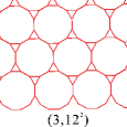
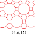
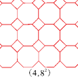
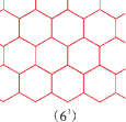
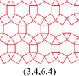
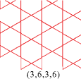
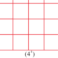
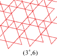
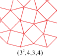
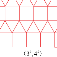
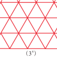
Figure 1: The 11 planar Archimedean lattices. The index gives the lattice name in the terminology explained in the text.

The dual transformation of a planar lattice is defined by adding one site at the center of each polygon and connecting these new sites to those of all neighboring polygons. This is a vertex-to-face, face-to-vertex, edge-to-edge transformation, and is reversible. The square lattice is manifestly self-dual and the honeycomb and triangular lattices are mutually dual. However, the dual lattices of the remaining eight Archimedean lattices are not Archimedean; clearly, the centering sites of the different polygons in these eight lattices have different connectivity. These are known as the Laves lattices, and they are shown in Fig. 2. The Laves lattices with integer average coordination number ${\bar{z}}$ play an important role in our considerations, and here we will study in detail the diced lattice ($D(3,6,3,6)$, ${\bar{z}}=4$), the Union-Jack lattice ($D(4,8^{2})$, ${\bar{z}}$ = 6), and the centered diced lattice ($D(4,6,12)$, ${\bar{z}}=8$). According to the four-color theorem four_coloring1 ; four_coloring2 , a planar lattice may only be bipartite (such as the diced lattice), tripartite (such as the Union-Jack lattice), or quadripartite. The lattices we investigate in this paper are either bipartite or tripartite.

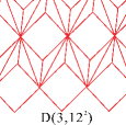
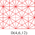
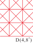
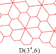
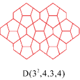
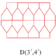
Figure 2: The set of Laves lattices, irregular planar lattices obtained as the non-Archimedean duals of the Archimedean lattices. The label gives the terminology for the dual Archimedean lattice.

A bipartite lattice contains only two sublattices of unconnected sites, and can be generated in one of two ways. One type is a lattice formed only by polygons with an even number of edges [square, honeycomb, $(4,8^{2})$, $(4,6,12)$, also the diced lattice ($D(3,6,3,6)$)]. On these lattices, each site A is connected only to sites of type B, and vice versa, and each polygon is composed alternately of A and B sites. The second type is the decorated lattice, formed by adding a site to each edge of a starting lattice. The original lattice sites and the decorating sites belong to different sublattices, and by taking a partial trace over the Potts variables on the decorating sites, the $q$-state AF Potts model on a decorated lattice can always be mapped onto a ferromagnetic Potts model with the same $q$ on the original lattice decorated_AF_F . The $q=2$ AF Potts (Ising) model on the bipartite lattice is always ordered at low temperature and disordered at high temperatures, with a finite-temperature phase transition. The $q=3$ AF Potts model on a bipartite lattice is more complicated, and its ground state can be disordered, critical, or ordered. Typical examples of these cases are respectively the honeycomb, square, and diced lattices. There is in general no finite-temperature phase transition for the $q=4$ AF Potts model on bipartite lattices.

Most of the planar lattices in Figs. 1 and 2 are tripartite. A tripartite lattice must contain some polygons with odd edge numbers (such as triangles or pentagons). The sublattices of a tripartite lattice may be determined uniquely if the lattice is formed purely by triangles [triangular, Union-Jack ($D(4,8^{2})$), centered-diced ($D(4,6,12)$)]. The $q=3$ Potts models on these lattices have complete AF long-range order in the ground state, with one of the three states on each sublattice. This order can be melted by thermal fluctuations, leading to a finite-temperature phase transition; if the lattice contains two inequivalent sublattices with unequal coordination numbers, two finite-temperature phase transitions are possible (Sec. VI). The sublattices for most tripartite lattices [kagome (3,6,3,6), square-kagome (4,$8^{2}$), (3,4,3,6), the dilute centered-diced lattices introduced in Sec. VII] are not unique, and $q=2$ and 3 AF Potts models may again have ordered, critical, or disordered ground states on these lattices. For the $q=2$ AF Potts model, any order in the ground state will be partial, because the model is frustrated on a tripartite lattice.

III Tensor-Based Numerical Methods

The development of numerical methods for condensed matter and lattice systems based on tensor-network representations Verstraete2008_AP57-143-224 is motivated by developments in quantum information theory, and a great deal of progress has taken place in the last five years. Tensor-based numerical methods have already been used to study spin Murg2005_PRL95-057206 ; jiang_2008_PRL ; Xie2009_PRL103-160601 ; Zhao2010_PRB81-174411 ; huihai_2012_prb ; Zhiyuan_PRX_2014 , bosonic Jordan2009_PRB79-174515 , and fermionic models Barthel2009_PRA80-042333 ; Kraus2010_PRA81-052338 , and to deal with quantum critical systems Vidal2007_PRL99-220405 and topological quantum phase transitions Gu2008_PRB78-205116 . They have been combined with Monte Carlo techniques Sandvik2007_PRL99-220602 to take advantage of the best features of both methods and they have been extended to deal with classical systems such as classical XY models Jifeng .

When dealing with models in classical statistical mechanics, the quantity expressed as the contraction of a tensor network is the partition function. In one dimension, this quantity is a product of matrices, which is easy to evaluate. In higher dimensions, the appropriate representation is by a network of tensors whose rank matches the coordination number of the lattice; in this situation, the dimension of the tensors obtained after each contraction step increases if the same amount of information is to be stored, and so a truncation is required to keep the contraction under control. A large number of methods has been developed to perform this truncation, including the tensor renormalization group (TRG) Levin2007_PRL99-120601 , second renormalization group Xie2009_PRL103-160601 ; Zhao2010_PRB81-174411 , infinite time-evolving block decimation (iTEBD) Vidal2007_PRL98-070201 ; Orus2008_PRB78-155117 , corner transfer matrix Orus2009_PRB80-094403 ; Or'us2012_PRB85205117 , plaquette renormalization group Wang2011_PRE83-056703 , and a renormalization-group method based on higher-order singular value decomposition (HOSVD) Xie2012_PRB86-045139 . Here we summarize three of these methods for pedagogical purposes, and during our analysis of AF $q$-state Potts models we considered a number of approaches in the process of optimizing our calculations, but at the end all of the numerical results presented in Secs. IV-VII were obtained using iTEBD.

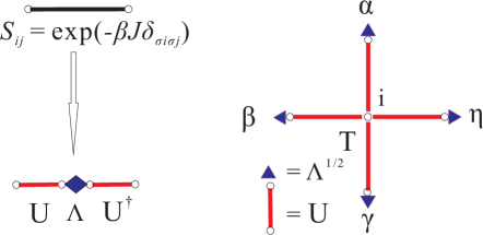
(a)             (b)

Figure 3: (Color online) Schematic representation of the expression of the partition function of the $q$-state Potts model as a tensor network. (a) Eigenvalue decomposition of the Boltzmann factor $S_{ij}$ for a bond. (b) Construction of the local tensor $T$ by contraction of four $U$ matrices and renormalization by the square root of the eigenvalues $\Lambda$.

III.1 Partition Function and Thermodynamics

It is always possible to find a tensor-network representation for the partition function of a classical model Zhao2010_PRB81-174411 ; Jifeng . In the example of the $q$-state Potts model on a square lattice, one may define the Boltzmann factor associated with each bond $\langle ij\rangle$ as

$$S_{ij}=\exp(-\beta J\delta_{\sigma_{i}\sigma_{j}}),$$ (2)

where $\sigma_{i}$ denotes the Potts variable on site $i$. As represented schematically in Fig. 3, an eigenvalue decomposition for $S$ yields

$$S_{ij}=\sum\limits_{\alpha}U_{i\alpha}\Lambda_{\alpha}U_{j\alpha},$$ (3)

where $U_{i\alpha}$ is a unitary matrix and $\alpha=0,1,\dots,q-1$ because $S_{ij}$ is a $q\times q$ matrix for the $q$-state Potts model. Now the partition function can be expressed as

$$Z=\sum\limits_{\{\sigma\}}\prod\limits_{\langle ij\rangle}S_{ij}\;\;=\;\;\sum\limits_{\{\alpha\}}T_{\alpha\beta\gamma\eta}T_{\alpha\epsilon\zeta\theta}\dots,$$ (4)

where

$$T_{\alpha\beta\gamma\eta}=\sum\limits_{i}U_{i\alpha}U_{i\beta}U_{i\gamma}U_{i\eta}(\Lambda_{\alpha}\Lambda_{\beta}\Lambda_{\gamma}\Lambda_{\eta})^{1/2},$$ (5)

i.e. as a network of tensors $T$ constructed from the bond eigenvalues and eigenvectors. The rank of $T$ is determined from the number of bonds per site of the tensor lattice, which is often the coordination number $z$ of Sec. II. From above, the bond dimension of each index is $q$. There are many ways to contract this tensor network and in this section we review the TRG/SRG and iTEBD methods, which represent respectively the two primary classes of technique, namely variational, renormalization-group approaches that converge to infinite size and power or projection approaches that are already (by translational invariance) in this limit.

III.2 TRG/SRG

The tensor renormalization group (TRG) Levin2007_PRL99-120601 is a real-space coarse-graining method proposed by Levin and Nave in 2007. After each coarse-graining step, both the topology of the lattice and the rank and dimension of the tensor remain the same, but the size of the lattice is only half (in general) of its original size. The method proceeds by first decomposing the tensor and then recombining new tensors, but the details depend on the lattice topology and are best illustrated by example.

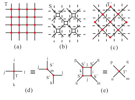
Figure 4: (Color online) Two TRG steps on the square lattice. (a) The original tensor network on the square lattice representing the partition function as in Eq. (4). (b) After a SVD of the local tensor following alternating “stretching” directions on the two different sublattices, the square-lattice tensor network is transformed to one on the Archimedean ($4$, $8^{2}$) lattice (Fig. 1). (c) Groups of four rank-3 tensors are then contracted to form one new rank-4 tensor on a lattice with half the number of sites of the original square lattice. (d) SVD of a local tensor, defined by Eq. (6). (e) Contraction of four rank-3 tensors into a rank-4 tensor, as defined by Eq. (7).

On the square lattice (Fig. 4), each iteration requires two steps. First the rank-4 site tensor is decomposed into two rank-3 auxiliary tensors, with a choice of indices following alternating “stretching” directions on the two different sublattices. Specifically, by combining two indices the rank-4 tensor becomes a matrix (rank-2 tensor) whose SVD yields a set of singular values, which are absorbed into the two unitary bond matrices. By expanding the combined index one obtains two rank-3 tensors,

$$T_{ijkl} = \sum_{m}U_{ij,m}\lambda_{m}V_{kl,m},$$

$$S^{1}_{ijm} = U_{ij,m}\sqrt{\lambda_{m}},$$ (6)

$$S^{2}_{klm} = V_{kl,m}\sqrt{\lambda_{m}},$$

where $U$ and $V$ are unitary matrices, and $\lambda$ is a diagonal singular-value matrix. The partition function is represented as a tensor network defined on the Archimedean $(4,8^{2})$ lattice (Fig. 1). If the dimension of the bond index for the tensor $T$ is $d$, the dimension of index $m$ is $d^{2}$ [Eq. (6)]. This bond dimension grows during the renormalization process and when $d=D$, the maximum bond dimension we can retain due to the limits set by our computational resources, a truncation is required to prevent divergence on repeated iteration. Here the natural approach is to cut the dimension of $m$ according to the relative sizes of the singular values and to keep the $D$ largest ones. The second step of the iteration is to contract the four rank-3 tensors on the $(4,8^{2})$ squares into a new rank-4 tensor,

$$T^{\prime}_{mnpq}=\sum_{ijkl}S^{1}_{ijm}S^{4}_{jkn}S^{2}_{klp}S^{3}_{liq},$$ (7)

as a result of which both the topology of the tensor network and the dimension of the local tensor are unchanged. Thus each iteration step forms a new square lattice whose tensor-network representation contains only half as many sites. If the iteration is repeated $n$ times, the size of the tensor network shrinks to $2^{-n}$ of the original, giving easy access to the thermodynamic limit by renormalization methods.

However, in the TRG approach the tensor is truncated according to its singular values, which is in essence a local approximation. In fact the same pair of sites is connected by (many) other paths in the lattice and a more consistent approach is to consider the effect of this “environment” in order to perform the truncation globally, which is the concept of the second renormalization group (SRG) method Xie2009_PRL103-160601 .

The partition function can be expressed as

$$Z=\rm{Tr}[T_{i}T_{i}^{e}]$$ (8)

where $T_{i}^{e}$ is the environment contribution, meaning that from all lattice sites other than $i$. It is not possible to deduce this environment tensor rigorously (as otherwise one would have a rigorous expression of the partition function, which is not available for most models), but its effect can be included optimally by truncating the local tensor $T_{i}$ in order to minimize the truncation error of $Z$. Specifically, a SVD of the environment tensor yields

$$T^{e}_{ij,kl}=\sum_{n}U^{e}_{ij,n}\Lambda^{e}_{n}V^{e}_{kl,n}$$ (9)

and thus the partition function becomes

$$Z = \rm{Tr}[TU^{e}\Lambda^{e}V^{e}]=\rm{Tr}[V^{e}TU^{e}\Lambda^{e}]$$ (10)

$$= \rm{Tr}[(\Lambda^{e})^{1/2}V^{e}TU^{e}(\Lambda^{e})^{1/2}].$$

If one defines

$$\tilde{T}_{n_{1}n_{2}}=(\Lambda^{e})^{1/2}_{n_{1}}V^{e}_{kl,n_{1}}T_{ij,kl}U^{e}_{ij,n_{2}}(\Lambda^{e})^{1/2}_{n_{2}},$$ (11)

then the partition function is

$$Z=\rm{Tr}\tilde{T}$$ (12)

and the minimization of its error is the same as minimizing that of $\tilde{T}$. By a further SVD,

$$\tilde{T}=\tilde{U}\tilde{\Lambda}\tilde{V}$$ (13)

and the truncation may be performed according to $\tilde{\Lambda}$. By substituting the truncated $\tilde{T}$ back into Eq. (11) one obtains

$$T=V^{e}(\Lambda^{e})^{-1/2}\tilde{T}(\Lambda^{e})^{-1/2}U^{e}$$ (14)

and thus the two new rank-3 tensors appearing at the first TRG iteration step are given in a fully consistent approach by

$$S^{1} = V^{e}(\Lambda^{e})^{-1/2}\tilde{U}(\tilde{\Lambda})^{1/2},$$ (15)

$$S^{2} = (\tilde{\Lambda})^{1/2}\tilde{V}(\Lambda^{e})^{-1/2}U^{e}.$$ (16)

Once the environment tensor has been obtained, one may then deduce and truncate the local tensor $T_{i}$, then follow the steps of TRG to update the tensors in the renormalized lattice and thus complete a full cycle of SRG iteration. Repeating this procedure leads finally to the partition function in the thermodynamic limit, from which full thermodynamic information may be obtained (Secs. IV and V). The SRG method was found to improve the precision of the free energy for the two dimensional Ising model by $2$ to $5$ orders of magnitude over the TRG result Xie2009_PRL103-160601 . Further details of the SRG technique may be found in Refs. Xie2009_PRL103-160601 and Zhao2010_PRB81-174411 .

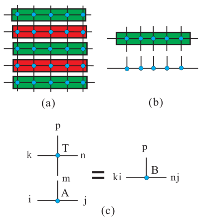
Figure 5: (Color online) Schematic representation of iTEBD. (a) Tensor network on the square lattice expressed as an infinite product of transfer matrices in the vertical direction, with each block a transfer matrix. (b) Definition of the transfer matrix and corresponding matrix-product state. (c) Local action of a transfer matrix on a matrix-product state as shown in Eq. (17)

III.3 iTEBD

A tensor network may be regarded as an infinite product of operators, or transfer matrices. Thus to contract the tensor network, one need only know the dominant eigenvector of the transfer matrix, and thus the power method can be used in the same way as in matrix algebra. This concept is the same as using a projection method to obtain the ground state of a quantum system. Let the local tensor (generalized transfer matrix) $T_{pkmn}$ be applied to the random but translationally invariant matrix-product state (MPS) $A^{m}_{ij}$, as represented in Fig. 5(a), then one obtains a new MPS [Fig. 5(c)]

$$\sum\limits_{m}T_{pkmn}A_{ij}^{m}=B_{(ki),(nj)}^{p}=B_{i^{\prime}j^{\prime}}^{m^{{}^{\prime}}}.$$ (17)

The dimension of the local matrix, $B$, for the new MPS is $qD$, where as in the TRG/SRG case (Sec. IIIB), $D$ is the maximum bond dimension that can be retained for the MPS and a truncation is required to keep the process under control. A unitary transformation of the new MPS places it in the canonical form canonical_form , which for an MPS with open boundary conditions is the form satisfying the conditions

1. $\sum\limits_{{}^{m_{i}}}A^{m_{i}}A^{m_{i}\dagger}=I\;\;\forall\;\;1\leq i\leq L$;

2. $\sum\limits_{{}^{m_{i}}}A^{m_{i}\dagger}\Lambda^{i-1}A^{m_{i}}=\Lambda^{i}\;\;\forall\;\;1\leq i\leq L$;

3. $\Lambda^{0}=\Lambda^{L}=1$, with all other $\Lambda^{i}$ being $D_{i}\times D_{i}$ diagonal matrices, which are positive, full-rank, and have $Tr{\Lambda^{i}}=1$.

Here $A^{m_{i}}$ is the local matrix on site $i$. The dimensions of the first and last matrices are respectively $1\times D_{1}$ and $D_{L}\times 1$. If the index $m$ of the local matrix $A^{m}_{ij}$ is taken as the index of the local basis for a quantum system, then the MPS represents the quantum state of a one-dimensional system,

$$|\varphi\rangle=\sum\limits_{\{m\}}\rm{Tr}(\prod\limits_{i}A^{m_{i}})|m_{1},m_{2},\dots m_{L}\rangle.$$ (18)

It can be proved that if the one-dimensional chain is cut between sites $i$ and $i+1$, the eigenvalue of the corresponding reduced density matrix is $\Lambda^{i+1}$.

The values of $\Lambda$ in the canonical form specify the truncation of the local matrix, which means retaining only the index corresponding to the $D$ largest $\Lambda$ matrices. This process is repeated, meaning repeated application of the operator $T_{pkmn}$, until the MPS has converged. The converged MPS is the approximate dominant eigenvector of the transfer matrix. The tensor network may thus be written as the contraction of an infinite product of these matrices and in this case the thermodynamic quantities can be obtained directly by diagonalizing the local matrix Vidal2007_PRL98-070201 ; Orus2008_PRB78-155117 .

For all of the models we study in this work (Secs. IV-VII), the final tensor network for the partition function is defined on the square lattice. Although every tensor network is uniform, meaning the local tensor is the same on each site, we use a two-sublattice MPS in all our calculations on this lattice in order to capture any possible spontaneous breaking of symmetry.

IV Entropy-Driven Phase Transitions

IV.1 Diced Lattice with $q=3$

The AF $q=3$ Potts model on the diced lattice provides an excellent example of an entropy-driven phase transition to a state of partial order, by which is meant order on a subset of the lattice sites. Thus we begin the presentation of both the physical ideas and our numerical results by considering this case. The diced lattice [Fig. 6(a)] is dual to the kagome lattice, and is composed of a triangular lattice of sites of one sublattice (A) decorated by centering sites (centered in each triangle) of the other sublattice (B). On this bipartite lattice, sites A are sixfold-coordinated by sites B ($z_{A}=6$) but sites B are only threefold-coordinated by sites A ($z_{B}=3$), whence the average coordination number is ${\bar{z}}=4$ and there are twice as many B sites as A sites ($N_{A}=N_{B}/2=N/3$).

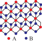
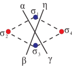
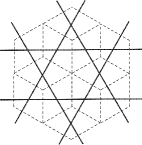
(a)        (b)        (c)

Figure 6: (Color online) (a) Diced lattice. A sites (red) have $z_{A}=6$, while B sites (blue) have $z_{B}=3$. (b) Definition of tensors for each unit cell of the diced lattice. (c) By introducing one tensor in each rhombus of the original diced lattice, as represented in panel (b), the partition function on the diced lattice (dashed lines) may be expressed as the contraction of a network of tensors defined on the sites of the kagome lattice (solid lines).

With AF interactions, neighboring sites favor different Potts states $\sigma_{i}$ (1). A three-state model on a bipartite lattice has redundant degrees of freedom with which to ensure that every bond is satisfied and the ground state will be highly degenerate. The two most obvious possibilities for partially ordered configurations minimizing the bond energy are as follows. One is that the A sites [red in Fig. 6(a)] order, choosing for example $\sigma_{i}(i\in A)=0$, leaving the B-sites (blue) to choose $\sigma_{i}(i\in B)=1$ or $\sigma_{i}(i\in B)=2$ at random. The other is that the B-sites order with the same $\sigma_{i}$ and the A sites are random. In both cases, ordering occurs only on a subset of the lattice sites, but every bond in the system can achieve its lowest energy, which is $0$. We comment that the combined set of all these ordered configurations does not exhaust the total possible ground-state configurations. However, these two types of partially ordered state contribute to a very large residual entropy in the ground state. At this point, simple physical intuition suggests that, on lowering the temperature, the A sublattice will order, not because these are the highly coordinated sites but because the number of states with the B sublattice disordered is much greater and therefore the entropy is maximized.

Of course this is the correct answer, and both the qualitative and quantitative details are well known in the literature. It was proven by Kotecky et al. Kotecky2008_PRL101-030601 that there is a finite-temperature phase transition in this model, and by calculating the sublattice magnetization using the Wang-Swendsen-Kotecky cluster algorithm these authors confirmed the existence of long-range partial order on the A sublattice at low temperatures.

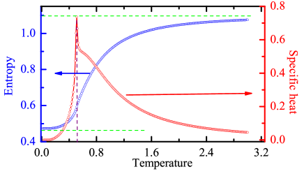
Figure 7: (Color online) Entropy and specific heat for the $q=3$ antiferromagnetic Potts model on the diced lattice. The results are obtained by iTEBD with $D=40$. The entropy is shown in blue, with the green dashed line denoting its low- and high-temperature limits. The specific heat, shown in red, has a divergence at the phase transition. The purple dashed line denotes the critical point obtained by Monte Carlo simulations Kotecky2008_PRL101-030601 .

This well-understood model for partial order provides an excellent example to benchmark our methods. Figure 6(b) illustrates the definition of the local tensor for this model. We first define the variable dual to $\sigma_{i}$ in each rhombus as

$$\alpha = \sigma_{2}-\sigma_{1}\pmod{q},$$

$$\beta = \sigma_{3}-\sigma_{2}\pmod{q},$$

$$\gamma = \sigma_{3}-\sigma_{4}\pmod{q},$$

$$\eta = \sigma_{4}-\sigma_{1}\pmod{q},$$ (19)

noting that these four dual variables are not independent, but are related by the constraint

$$\alpha+\beta-\gamma-\eta=0\pmod{q}.$$ (20)

The local tensor on the dual lattice is

$$T_{\alpha\beta\gamma\eta}=\exp[-\frac{\beta}{2}(\delta_{\alpha,0}+\delta_{\beta,0}+\delta_{\gamma,0}+\delta_{\eta,0})]$$ (21)

and defines a tensor network on the kagome lattice. This can be reconnected to a square-lattice tensor network by SVD Zhao2010_PRB81-174411 and the iTEBD method is used to contract the network.

The quantities required for a basic characterization of the thermodynamic response of a system are the free energy

$$F=-k_{\rm B}T\ln Z,$$ (22)

the entropy

$$S(T)=-\frac{\partial F}{\partial T}$$ (23)

and the specific heat

$$C(T)=-T\frac{\partial^{2}F}{\partial T^{2}}.$$ (24)

We have calculated these quantities, either from $Z$ by RG methods (TRG/SRG, Sec. IIIA) or directly by projection methods (iTEBD, Sec. IIIB); Fig. 7 shows our results for the entropy and the specific heat, which were published previously in Ref. Chen2011_Phys.Rev.Lett.107-165701 . The strong divergence of the specific-heat curve indicates the occurrence of a second-order phase transition. By analyzing the thermodynamic quantites alone, we obtained a transition temperature $T_{c}/J=0.508(1)$; however, a detailed consideration of the structure of the local tensor can be used to obtain a very much more accurate estimate of $T_{c}$ rwxcnx . The Monte Carlo result is $T_{c}/J=0.507510(8)$ Kotecky2008_PRL101-030601 , a value lying within the error bar of the thermodynamic tensor-network result and therefore validating the method.

The entropy provides some straightforward insight into the nature of the low-temperature phase. If the minority (A-sublattice) sites are ordered but the majority (B-sublattice) sites are disordered with a choice of the two remaining Potts states, the total number of states in the ground manifold is $2^{N_{B}}$, where $N_{B}=2N/3$ for a system of $N$ sites. The entropy per site would therefore be $S_{\rm d}^{A}(0)=(2/3)\ln 2=0.462098$. In contrast, if the B-sublattice is ordered, the entropy per site is only $S_{\rm d}^{B}(0)=(1/3)\ln 2=S_{\rm d}^{A}(0)/2$. We indeed conclude that a state of A-sublattice order will be selected. The zero-temperature limit of the entropy we calculate is $S_{{\rm d},q=3}(0)=0.473839$, which is slightly larger than the ideal value $S_{\rm d}^{A}(0)$, indicating an additional minor contribution from further spin configurations in the ground manifold where the A sites continue to fluctuate. The “ideal” low- and high-temperature limits, $S_{\rm d}^{A}(0)=(2/3)\ln 2$ and $S_{\rm d}(\infty)=\ln 3$ are shown by the green dashed lines in Fig. 7.

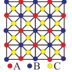
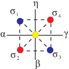
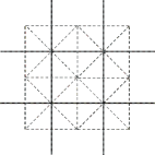
(a)        (b)        (c)

Figure 8: (Color online) (a) Union-Jack lattice. Sites in sublattices A (red circles) and B (blue) have coordination numbers $z_{A}=z_{B}=8$, while those in sublattice C (yellow) have $z_{C}=4$. (b) Definition of tensors for each unit cell of the Union-Jack lattice; the center site (yellow) is denoted $\sigma_{5}$ in the text. (c) By introducing one tensor in each unit cell of the original Union-Jack lattice, as represented in panel (b), the partition function of the Union-Jack lattice (dashed lines) is expressed after summation over the center sites [(b) and Eq. (26)] as the contraction of tensors defined on the sites of the square lattice (solid lines).

IV.2 Union-Jack Lattice with $q=4$

A considerably more challenging case of partial ordering is found in the Union-Jack lattice. This is a square lattice with additional center sites in each square, shown in Fig. 8(a). Sites in the two sublattices of the square lattice are each eightfold-coordinated, $z_{A}=z_{B}=8$, while those on the centers have $z_{C}=4$; because there are twice as many C sites as A or B sites, $N_{A}=N_{B}=N_{C}/2=N/4$, the system has an integral average coordination, ${\bar{z}}=6$. One may therefore expect some comparison with the triangular lattice, where $z=6$ and $q_{c}=4$, making (Sec. II) the 4-state Potts model on the triangular lattice critical at $T=0$.

To consider the possibility of partially ordered states minimizing the bond energy, we begin with one square unit cell. After assigning a Potts state ${\sigma_{i}}$ to the center site, there are three other states for the four corner sites, and thus at least one of the diagonal pairs must be in the same state. This motivates the possibility of long-range order on just one of the A or B sublattices, which could also be anticipated from the previous subsection.

To determine the local tensor in a tensor-network formulation, we first define the variable dual to $\sigma_{i}$ in the same way for the diced lattice in Eq. (19). The most straightforward way to proceed is to trace out the Potts variable $\sigma_{5}$ in the middle of the square by introducing a temporary variable

$$\theta=\sigma_{1}-\sigma_{5}\pmod{q},$$ (25)

in terms of which the local tensor is

$$T_{\alpha\beta\gamma\eta} = e^{-\frac{\beta}{2}(\delta_{\alpha,0}+\delta_{\beta,0}+\delta_{\gamma,0}+\delta_{\eta,0})}$$ (26)

$$\times\sum_{\theta}e^{-\beta(\delta_{\theta,0}+\delta_{\theta+\alpha,0}+\delta_{\theta+\alpha+\beta,0}+\delta_{\theta+\eta,0})}.$$

The resulting square-lattice tensor network is then handled optimally by the iTEBD method.

The presence of partial order is indicated by a phase transition. The entropy and especially the specific-heat curves illustrated in Fig. 9(a) show no apparent discontinuities, and could on cursory inspection be taken as a sign that the model is at best critical, with $q_{c}=4$. However, a sufficiently detailed investigation of the specific heat, shown in Fig. 9(b), reveals that it is in fact discontinous, and this was one of the key results of Ref. Chen2011_Phys.Rev.Lett.107-165701 . Very sophisticated calculations were required, by two different tensor-based approaches (Sec. III) and using a systematic increase in the tensor dimension, which in Fig. 9(b) we also denote by $D$, to extract of the behavior of this feature. We were able to conclude that the discontinuity does remain finite on extrapolating $D\rightarrow\infty$, and that the partial ordering transition occurs at a temperature $T_{c}/J=0.339(1)$. The immediate question is why this transition should be so weak while that in the diced lattice is so strong. The immediate answer is that this should be evidence of a strong competition between candidate partially ordered states, for example those with only A-sublattice order and those with only B-sublattice order, and that this competition almost prevents the system from ordering at all.

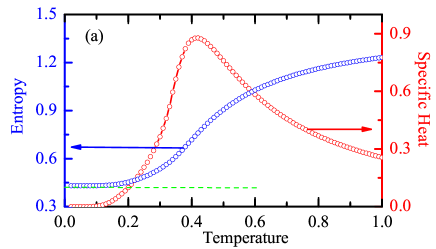
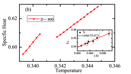
Figure 9: (Color online) (a) Entropy (blue) and specific heat (red) of the AF $q=4$ Potts model on the Union-Jack lattice. The dashed green line is the entropy derived from the $q=3$ Potts model on the decorated square lattice, which is relevant (see text) if either the A or the B sublattice is ordered. (b) Detail of the specific heat, showing a subtle discontinuity at the transition to partial order. Inset: scaling of the specific-heat discontinuity as a function of tensor dimension $D$.

To examine the partially ordered ground state in more detail, we begin by considering the entropy. For simultaneous order on both A and B sublattices, for example $\sigma_{i}=0$ on A and $\sigma_{i}=1$ on B, sites on sublattice C may choose $\sigma_{i}=2$ or $3$ at random to satisfy every bond. Because there are $2^{N/2}$ such states, one would expect to find $S_{AB}(0)=(1/2)\ln 2=0.346573$. Our numerical result for the zero-temperature entropy is very much larger, $S_{\rm UJ}(0)=0.43097359$, indicating that configurations with both A- and B-sublattice order do not play a significant role in the ground state. If only A sublattice sites are ordered in one state, then the B and C sites form a decorated square lattice with three remaining degrees of freedom. These sites are clearly highly energetically correlated, but if this hypothesis for the ground state is relevant then their behavior should be given by that of the AF $q=3$ Potts model on the decorated square lattice. If the zero-temperature entropy of this model is expressed as $S_{{\rm DS},q=3}(0)=\ln\zeta$, the requirement for the ground state to be dominated by configurations with partial order only on a single sublattice is that $\zeta^{3N/4}>2^{N/2}$, or $\ln\zeta>(2/3)\ln 2=0.462098$. Our tensor-network calculation Chen2011_Phys.Rev.Lett.107-165701 gives the result $S_{{\rm DS},q=3}(0)=0.56106936$ and thus the condition is clearly satisfied, meaning that partial order appears only on one of the sublattices (A or B). Continuing with the approximation of a decorated square lattice, one would expect to find that $S_{\rm UJ}(0)=3S_{{\rm DS},q=3}(0)/4=0.420802$. The deviation between this value and the exact numerical result above quantifies the contributions to the ground manifold of configurations where neither sublattice A nor B is ordered.

The qualitative knowledge that a highly degenerate ordered state exists for the $q=4$ Potts model on the Union-Jack lattice has immediate connections to a number of other problems in statistical physics. Because the fundamental unit of the Union-Jack lattice is a triangle, there is a mapping between the 4-state Potts model on this lattice and the 3-bond coloring problem on its dual lattice triangular_qc , which is the 4-8 lattice [marked as (4,$8^{2}$) in Fig. 1]. If the four states $\sigma_{i}=0,1,2,3$ are represented by the vertices of a tetrahedron, then three different colors are required to mark the inequivalent pairs of edges. At zero temperature, every triangle of the Union-Jack lattice must take one of the configurations of the faces of this tetrahedron, with no two bonds of the same color touching. After the dual transformation, the bonds sharing the same vertex on the 4-8 lattice are always of different colors, and the manifold of solutions to the 3-bond coloring problem is established. The total number of configurations for the ground state on the 4-8 lattice, $W_{4-8}^{N_{4-8}}$, has been calculated exactly by mapping the bond coloring problem further to a solved model on the square lattice Fjaerestad2010_J.Stat.Mech.2010-P01004 . The result is $W_{4-8}=1.24048$, and because $N_{4-8}=2N_{\rm UJ}$, one may deduce that $S_{\rm UJ}(0)=2\ln W_{4-8}=0.430997$, which coincides to two parts in $10^{-5}$ with the result we obtain numerically.

Further, the bond-coloring problem on the 4-8 lattice is equivalent to the fully-packed loop (FPL) model on the same lattice. FPL models consider all configurations of non-crossing closed loops that may be drawn along the edges of the lattice, with every vertex visited by one loop. A loop covering on the 4-8 lattice may be derived from a 3-bond (red, blue, green) coloring by drawing loops on those edges which are red or blue, but not on green edges. Thus every vertex will be visited by a loop, no loops may touch, and because each vertex has two red or blue edges then all loops are closed. The correspondence on the 4-8 lattice between fully-packed-loop and 3-bond-coloring models is well established Fjaerestad2010_J.Stat.Mech.2010-P01004 . The partition function of a FPL model is

$$Z=\sum_{G}n^{N_{L}},$$ (27)

where the fugacity $n$ is the weight of every loop, $N_{L}$ is the number of loops, and the sum is over all configurations $G$ of loops. Because the edges of each loop may be ’red-blue-red-blue’ or ’blue-red-blue-red,’ the fugacity is $n=2$. The $n=2$ FPL model is known Jacobsen_loop to be critical on both the square and the honeycomb lattices, but not on the 4-8 lattice, which is completely consistent with the existence of partial order on the 4-8 lattice.

Finally, if a vertex is placed at the midpoint of every edge of the 4-8 lattice, and all vertices on neighboring bonds are connected, one obtains the square-kagome lattice triangular_qc , a non-Laves lattice composed of triangles, squares, and octagons. This is a bond-to-site transformation, and so the 3-bond coloring model on the 4-8 lattice is equivalent to the 3-vertex coloring model on the square-kagome lattice. Thus at zero temperature the AF $q=3$ Potts model on the square-kagome lattice is equivalent to the AF $q=4$ Potts model on the Union-Jack lattice.

IV.3 Centered Diced Lattice with $q=4$ and 5

If an extra site is added to the center of each rhombus in the diced lattice and is connected to all its neighbors, one obtains the centered-diced lattice, also known as the bisected-hexagonal or $D(4,6,12)$ lattice [Fig. 10(a)]. Like the Union-Jack lattice, the centered diced lattice is tripartite, is composed entirely of triangles and has ${\bar{z}}=6$, with sublattice site coordinations $z_{A}=12$, $z_{B}=6$, and $z_{C}=4$ and site numbers $N_{A}=N_{B}/2=N_{C}/3=N/6$.

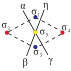
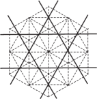
(a)        (b)        (c)

Figure 10: (Color online) (a) Centered diced lattice: $z_{A}=12$ (red), $z_{B}=6$ (blue), and $z_{C}=4$ (yellow). (b) Definition of tensors for each unit cell of the centered diced lattice. (c) By introducing one tensor in each unit cell of the original centered diced lattice, as represented in panel (b), the partition function on the centered diced lattice (dashed lines) may be expressed as the contraction of tensors defined on each site of the kagome lattice (solid lines).

From the intuition developed for irregular lattices in the preceding subsections, one expects that a $q=4$ Potts model on this lattice will show an ordering transition to a state of partial order on the highly-coordinated A sublattice. The lack of competition between different ordering configurations suggests that the transition should be rather robust, more similar to that in the diced lattice than to the Union-Jack case. Indeed we presented these considerations as predictions in Ref. Chen2011_Phys.Rev.Lett.107-165701 and we provide the complete quantitative details here.

By working with a centered four-site unit cell, the local tensor for the centered diced lattice is same on the Union-Jack lattice (26), with the difference appearing only in the topology of the tensor network. By an SVD transformation of the same type as that made in our treatment of the diced lattice Zhao2010_PRB81-174411 , we obtain a square-lattice tensor network and compute the thermodynamic quantities by the iTEBD method.

The entropy and specific heat of the $q=4$ case are shown in Fig. 11(a). Indeed the specific heat demonstrates the presence of a very robust transition at $T_{c}/J=0.56(1)$. Here and henceforth we quote transition temperatures with an accuracy of $0.01J$, because our primary focus is the qualitative presence and nature of the transition, but we stress that our tensor-based methods allow the value of $T_{c}$ to be computed to very high accuracy if required rwxcnx . As above, the nature of the partially ordered state on the centered diced lattice may also be inferred from the low-temperature limit of the entropy. If indeed only the A sublattice is ordered, the sites of sublattices B and C form a $q=3$ decorated honeycomb lattice and the zero-temperature entropies would be given by $S_{{\rm cd},q=4}(0)=5S_{{\rm dh},q=3}(0)/6$. Our calculations give $S_{{\rm cd},q=4}(0)=0.510380$ and $5S_{{\rm cd},q=3}(0)/6=0.510128$, demonstrating that partial order only on the A sublattice is in fact realized very accurately for the $q=4$ model.

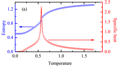
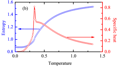
Figure 11: (Color online) Entropy and specific-heat of the isotropic AF Potts model on the centered diced lattice. The results are obtained by iTEBD with $D=40$. (a) $q=4$. (b) $q=5$.

As in the case of the Union-Jack lattice, the $q=4$ Potts model on the centered diced lattice is also related to a number of other statistical problems. At zero temperature, it may be mapped to the 3-bond coloring problem on the Archimedean 4-6-12 lattice (Fig. 1), and to an $n=2$ FPL model on this lattice. By similar manipulations it may also be mapped to an $n=3$ close-packed-loop (CPL) model on the kagome lattice, to a six-vertex model on the kagome lattice, and to a ferromagnetic $q=9$ Potts model at a temperature $e^{\beta J}=4$ on both the honeycomb and triangular lattices Deng2011_Phys.Rev.Lett.107-150601 . All of these problems are known to be non-critical, in agreement with our conclusion that the system has quite robust, if partial, long-range order.

We conclude this section by extending our considerations to the $q=5$ Potts model on the centered diced lattice, whose entropy and specific heat are illustrated in Fig. 11(b). A finite-temperature phase transition occurs at $T_{c}/J=0.33(1)$, and its signal remains robust even though its critical temperature is significantly lower than the $q=4$ case. As above, the nature of the partial order may be verified by comparing the zero-temperature entropy of the model with that of the decorated honeycomb lattice formed by the sites of sublattices B and C, which have $q=4$ remaining Potts states, in the event of full A-site order. We obtain $S_{{\rm cd},q=5}(0)=0.873635$ and $5S_{{\rm dh},q=4}(0)/6=0.867564$, indicating a minor but discernible entropic contribution from additional configurations minimizing the bond energy without A-site order.

To our knowledge, the centered diced lattice is the only planar lattice yet known to have long-range order when $q=5$, and therefore it possesses the largest $q_{c}$ known in two dimensions. Our initial study of irregular lattices Chen2011_Phys.Rev.Lett.107-165701 was followed up by a further analysis of the centered diced geometry Deng2011_Phys.Rev.Lett.107-150601 , which predicted that $q_{c}=5.397(5)$.

V Order parameter

The most accurate way to characterize the partially ordered state is to determine the order parameter, which is the sublattice magnetization $M$. Vanishing of the order parameter at the phase transition also offers an alternative to the specific heat for determining the presence of a transition and the exact value of $T_{c}$. The fact that $M=-\partial\ln Z(H)/\partial H$ is only a first derivative of the free energy, while the specific heat is a second derivative, makes it possible to determine the location of the transition from $M$ using significantly larger values of the tensor bond dimension $D$.

To calculate the sublattice magnetization most efficiently, we add a very small field $H$ to one sublattice (which we are able to choose from the results of Sec. IV), as shown in Eq. (1). We compute the quantity

$$M=\frac{1}{N_{\cal L}}\langle\sum\limits_{i\in{\cal L}}\delta_{\sigma_{i},0}\rangle-\frac{1}{q},$$ (28)

which is the probability of finding the $N_{\cal L}$ sites of sublattice ${\cal L}$ in the state $\sigma_{i}=0$ selected by the field term. The average value $1/q$ is subtracted to ensure that the order parameter is zero when the system is in its high-temperature disordered phase.

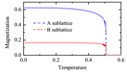
Figure 12: (Color online) Magnetization of the A sublattice for the AF $q=3$ Potts model on the diced lattice. The results are obtained by iTEBD with $D=40$. Shown also is the probability of sites on the B sublattice being in one Potts state $\sigma_{i}$ different from that of the A sites.

V.1 Diced Lattice with $q=3$

Figure 12 shows the magnetization of the AF $q=3$ Potts model on the diced lattice. We show results not only for the probability of finding $\sigma_{i}=0$ on the A sublattice but also for the probability of finding $\sigma_{i}=1$ or 2 on the B sublattice. Both curves exhibit the typical behavior of a second-order phase transition, with the order parameter (determined from the A sublattice) going continuously to zero at $T_{c}$. The low-temperature limiting value for the magnetization of the A sublattice is $M_{\rm d}(0)=0.62426$, somewhat lower than the perfect-order result $M_{\rm d}^{0}(0)=2/3=1-1/3$, from which we deduce that the ground state of the diced lattice retains fluctuations suppressing the partially ordered state by approximately 6%.

The B-sublattice quantity is neither a magnetization nor an order parameter, but its value is $0.166202$, which is very close to the value $1/6=1/2-1/3$ obtained in the event of a completely random distribution of the B sites between states $\sigma_{i}=1$ and 2. Indeed, if 6% of the A-sublattice sites are not ordered with $\sigma_{i}=0$, the density of B-sublattice sites with no $\sigma_{i}=0$ neighbor is of order $0.06^{3}$; because these contain only limited information, we do not present calculations for the non-ordered sublattices in the other systems discussed in this section.

Thus the entropy and the sublattice magnetization both demonstrate that the low-temperature phase is a state of partial order in which A-sublattice sites order in one Potts state while B-sublattice sites are disordered, choosing the remaining two Potts states at random and contributing to the very high ground-state entropy. The sublattice magnetization provides clearer insight into the deduction made from the entropy in Sec. IV that there exist ground-state configurations where the A sublattice is not fully ordered, and these configurations cause the departures from the ideal values observed in our exact numerical results.

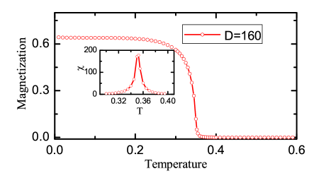
Figure 13: (Color online) Magnetization of the A sublattice for the AF $q=4$ Potts model on the Union-Jack lattice. Inset: corresponding susceptibility $\chi=\partial M/\partial H$.

V.2 Union-Jack Lattice with $q=4$

We computed the magnetization and susceptibility of the $q=4$ Potts model on the Union-Jack lattice in Ref. Chen2011_Phys.Rev.Lett.107-165701, , and show the results in Fig. 13 to retain the completeness of this paper. Despite the fact that the phase transition is very difficult to identify in the specific heat (Fig. 9), it is clearly visible in the magnetization as a rapid but continuous drop of the sublattice magnetization. While the tensor-network calculation of $M(T)$ can indeed be performed with significantly higher values of $D$ than for $C(T)$, it is largely the nature of $M$ as a true order parameter that makes it a superior indicator of the phase transition. A further robust indicator of the transition is the susceptibility, defined as $\chi=\partial M/\partial H$, which diverges on approaching the transition. However, we comment that the temperature grid used in the preparation of Fig. 13 does not allow a determination of the critical temperature $T_{c}/J=0.339(1)$ more accurate than the result of the detailed analysis performed in Sec. IV. The low-temperature limiting value we compute for the order parameter is $M_{\rm UJ}(0)=0.6428$, which is some 14% less than the ideal value $3/4=1-1/4$. The sublattice magnetization provides a clear indication of the discrepancy between the exact result and the state of perfect A-sublattice order. While we are unaware of an analytical relationship between the magnetization discrepancy and the entropy discrepancies calculated in Sec. IVB, our calculations allow a quantitative determination of this connection for all lattices, and similar results will appear again in Sec. VII.

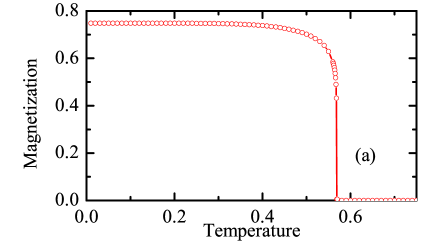
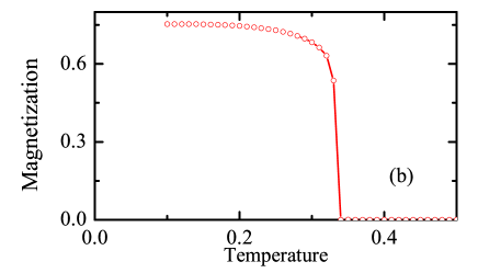
Figure 14: (Color online) Magnetization of the A sublattice for the AF Potts model on the centered diced lattice. The results are obtained by iTEBD with $D=30$. (a) $q=4$. (b) $q=5$.

V.3 Centered Diced Lattice with $q=4$ and 5

We conclude this section by computing the magnetization of the A sublattice for the centered diced lattice, which is presented in Fig. 14(a) for $q=4$ and in Fig. 14(b) for $q=5$. Both curves show clear, second-order phase transitions occurring respectively at critical temperatures $T_{c}/J=0.56(1)$ and 0.33(1). The low-temperature limit of the magnetization for the $q=4$ case is $M_{{\rm cd},q=4}(0)=0.74845$, which is very close to the ideal value $0.75=1-1/4$, as expected for a system with the very robust one-sublattice partial order suggested by our entropy calculations for the decorated honeycomb lattice (Sec. IVC). For the $q=5$ model, we find that $M_{{\rm cd},q=5}(0)=0.7540$ in comparison with an ideal value of $0.80=1-1/5$, illustrating clearly a 5.5% departure from perfect order arising as a consequence of the very high degeneracy of ground-state configurations in this high-$q$ case.

VI Intermediate Partial Order and Multiple Phase Transitions

In the preceding sections we have considered only models with the same interaction $J$ between Potts variables on every pair of sites [Eq. (1)], i.e. despite the inequivalent sites, the bonds have equivalent strengths. In this section, we relax this constraint to illustrate the phenomenon of multiple phase transitions within a single Potts model. These can occur on a number of different lattices and for specific $q$ values whose common feature is that states of partial order appear at intermediate temperatures, between complete order at low temperature and complete disorder at high temperature.

VI.1 Union-Jack Lattice with $q=2$

The AF $q=2$ Potts model is equivalent to the Ising model, which has been solved exactly on the Union-Jack lattice Vaks1966_JETPLetters22-820 . We consider the system with inequivalent interactions, taking those between A and B sites to have a strength $J_{AB}$ and those of C sites to both A and B sites to have a strength $J_{C}$. If the sign of $J_{C}$ is exchanged, and at the same time change the definition of the Potts variable $\sigma_{i}$ on the C sublattice is changed to $-\sigma_{i}$, the model is unchanged. Thus the phase diagram is symmetrical about $J_{C}=0$ and for simplicity we consider only ferromagnetic values of $J_{C}$ ($J_{C}<0$). When $J_{AB}$ is ferromagnetic, the model has very simple behavior, and in the following discussion we consider only the case where $J_{AB}$ is AF ($J_{AB}>0$).

If one considers a single square unit cell, in the limit of large $J_{AB}$, sublattices A and B will adopt an AF ordered configuration and sublattice C will be chosen randomly, as represented in Fig. 15(a), giving a ground-state energy per unit cell of $-2J_{AB}$. In the opposite limit of large $|J_{C}|$, the minimum energy is obtained when all the sites in the lattice are ferromagnetically ordered, as shown in Fig. 15(b), giving a ground-state energy per cell of $-4|J_{C}|+2J_{AB}$. By equating the two limits, one might expect a transition to occur when $J_{AB}=|J_{C}|$.

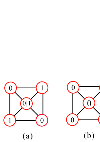
Figure 15: Ground-state configurations for the $q=2$ Potts model on a single unit cell of the Union-Jack lattice. (a) $J_{AB}\gg|J_{C}|$. (b) $|J_{C}|\gg J_{AB}$.

The local tensor for this model is defined as in Eq. (26). If we choose a parameter ratio far from either limit of the previous paragraph, $J_{AB}=1.0$, $J_{C}=-1.05$, our results for the entropy, specific heat, and sublattice magnetizations show complex behavior (Fig. 16). From the specific heat it appears that two phase transitions occur, with critical temperatures of $T_{c1}=0.145(5)$ and $T_{c2}=0.635(5)$. However, the exact result Vaks1966_JETPLetters22-820 contains not two but three finite-temperature phase transitions for this parameter ratio. On cooling from the high-temperature disordered phase, there is a transition to an AB-sublattice AF phase with the C sublattice disordered, then another, very narrow, phase of complete disorder, and at low temperatures a ferromagnetic phase. The three critical temperatures are respectively $0.6348196$, $0.1446858$, and $0.1438721$.

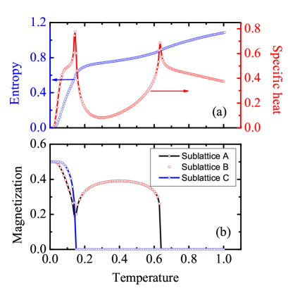
Figure 16: (Color online) Thermodynamic properties of the $q=2$ Potts model on the Union-Jack lattice, calculated with coupling constants $J_{AB}=1.0$ and $J_{C}=-1.05$. The results are obtained by iTEBD with $D=30$. (a) Entropy and specific heat. (b) Magnetizations of the A, B, and C sublattices.

To interpret these results we note from above that, if $|J_{C}|>J_{AB}$ the ground state should be ferromagnetic on all the three sublattices [Fig. 15(b)]. However, this is a state with zero entropy, whereas the AF configuration of the A and B sublattices [Fig. 15(a)] has a higher energy (only marginally higher for $J_{C}/J_{AB}=-1.05$) but a massive degeneracy of $2^{N/2}$ in an $N$-site lattice. Thus a moderate temperature may stabilize this type of partially ordered configuration, with complete C-sublattice disorder, before order is lost on all three sublattices at higher temperatures. The most striking aspect of the phase diagram is that all transitions are continuous (second-order), but the AB-sublattice AF configuration is so different from the low-temperature ferromagnetic configuration that the order parameter must vanish completely between the two phases. The width of this regime of “fully frustrated disorder” is, however, so narrow that it can only be resolved in our numerical calculations by specific targeting rwxcnx . We note in addition that the energy balance allowing this entropy-driven reordering to occur is also rather delicate, arising only for coupling values $1<|J_{C}/J_{AB}|<1.09(1)$.

To verify the nature of the ordered and partially ordered phases, we also calculate the sublattice magnetization and the results are presented in Fig. 16(b). We remind the reader that the magnetization is computed [Eq. (28)] with an explicit assumption for the Potts state $\sigma_{i}$ of each sublattice. With the assumption of low-temperature ferromagnetism and an intermediate AF state, the numerical results confirm the above analysis. We observe in the low-temperature state that the frustrated AB-sublattice order is suppressed by thermal fluctuations more rapidly than is the satisfied C-sublattice order.

The existence of multiple phase transitions in this model has been discussed Fradkin_PRA14 in a general framework of competing effective interactions between spin pairs arising due to paths with different numbers of bonds. We stress that, although this is the only model we consider in this paper with an explicit frustration, this frustration is resolved in favor of one (fully ordered) configuration in the ground state, which is nevertheless supplanted at finite temperatures by an entropically driven, partially ordered state of a very different local nature, without altering the frustration parameter.

VI.2 Union-Jack Lattice with $q=3$

We turn to the $q=3$ Union-Jack lattice and focus on the fully AF regime ($J_{AB}>0$, $J_{C}>0$ ). Because this lattice is tripartite and there is a unique way of dividing all the sites into three disconnected sublattices, the ground state of the $q=3$ AF model is expected to be a traditional three-sublattice AF ordering of the type shown in Fig. 17(a), but the fact that this is a state of zero entropy suggests the possibility of more complex physics at finite temperatures.

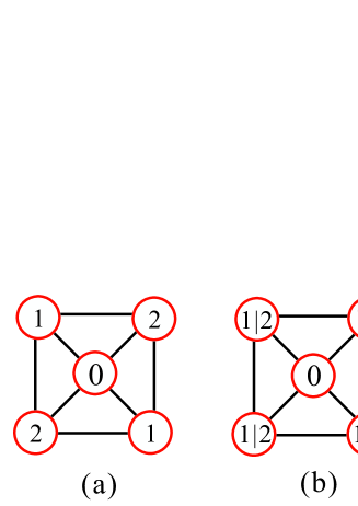
Figure 17: Configurations of the AF $q=3$ Potts model on a single unit cell of the Union-Jack lattice. (a) Three-sublattice AF-ordered ground-state configuration. (b) Configuration for the intermediate phase of partial order arising for $J_{C}/J_{AB}>2.2$.

To investigate this situation, we compute the entropy, specific heat, and sublattice magnetizations for a range of values of the parameter ratio $J_{C}/J_{AB}$. The definition of the local tensor is the same as in the $q=2$ case [Eq. (26)]. Figure 18 shows our results for $J_{AB}=1$ and $J_{C}=5$, where again two finite-temperature phase transitions are clearly visible in the specific heat [Fig. 18(a)], with critical temperatures $T_{c1}=1.10(1)$ and $T_{c2}=1.89(1)$. In the absence of an exact solution for this model, we deduce the nature of the phases at low and intermediate temperatures by calculating the sublattice magnetizations for the same parameters, as shown in Fig. 18(b).

At low temperatures, the system adopts the three-sublattice AF configuration as expected. However, when the temperature exceeds $T_{c1}$, only the C-sublattice order is preserved but the A- and B-sublattice order is destroyed by thermal fluctuations. Sites in these two sublattices do not become completely random but remain “polarized” by their strong AF interaction with the C sites; thus if the C sublattice has $\sigma_{i}=0$, the A and B sites have a random choice between $\sigma_{i}=1$ and 2, a result reflected in their finite magnetization of approximately $1/6=1/2-1/3$ in the regime $T_{c1}<T<T_{c2}$ [Fig. 17(b)]. At temperatures $T>T_{c2}$, entropic demands destroy the C-sublattice order as well, driving the system into the fully disordered phase.

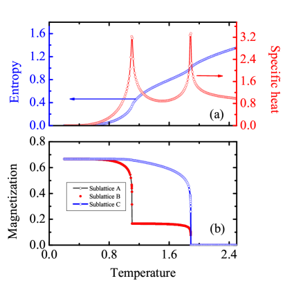
Figure 18: (Color online) Thermodynamic properties of the $q=3$ Potts model on the Union-Jack lattice, calculated with coupling constants $J_{AB}=1.0$ and $J_{C}=5.0$. The results are obtained by iTEBD with $D=30$. (a) Entropy and specific heat. (b) Magnetizations of the A, B, and C sublattices.

For a complete understanding of these phenomena, in Fig. 19 we show the phase diagram of the full parameter space. In the regime of large $J_{C}$, there are always two phase transitions, of which the lower one ($T_{c1}$) approaches the value $1.13$ as $J_{C}\rightarrow\infty$. $T_{c}/J=1.13$ is the transition temperature of the Ising model on the square lattice square_exact , and this is the model for the behavior of the AB-sublattice system when dominant $J_{C}$ bonds enforce for example $\sigma_{i}=0$ on all C sites, leaving a $q=2$ Potts degree of freedom on the A and B sites. This is fully consistent with the discussion above for the nature of the first transition, it means that $T_{c1}$ depends only on the coupling between A and B sites ($J_{AB}$), and it means that the lower transition is in the universality class of the Ising model.

The upper transition is the loss of C-sublattice order and therefore $T_{c2}$ scales linearly with $J_{C}$ when this becomes large. A linear fit using the data from $J_{C}=3$ to $J_{C}=10$ gives the form $T_{c2}=0.41(2)J_{C}+0.292(3)$. This transition has the universality of the ferromagnetic Ising model. As $J_{C}/J_{AB}$ becomes smaller, the behavior becomes more complex and the two transitions merge to a single one at $J_{C}\simeq 2.2$. One may anticipate that for very small values of $J_{C}$, a further type of intermediate phase could appear in which the A and B sites retain AF order but the C sites become random for entropic reasons. However, in our calculations we find only that $T_{c}\rightarrow 0$ as $J_{C}\rightarrow 0$, consistent with the fact that, when $J_{C}=0$, one obtains the $q=3$ Potts model on the square lattice, which is known to be critical at zero temperature Salas1998_JSP92-729 .

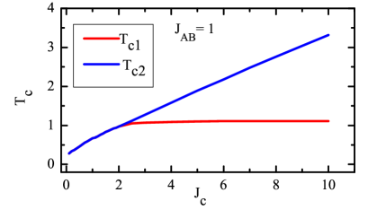
Figure 19: (Color online) Phase diagram of the $q=3$ Potts model on the Union-Jack lattice. The transition from full to partial order is shown in red (light grey) and from partial order to disorder in blue (dark grey). The two transitions merge for $J_{C}<2.2$. $J_{AB}$ is fixed to $1$.

VI.3 Centered Diced Lattice with $q=3$

We complete our analysis of intermediate-temperature partial order by considering the centered diced lattice with $q=3$. In common with the Union-Jack lattice, this geometry is tripartite with only one way of dividing all the sites into three disconnected sublattices and again one expects that the ground state should display three-sublattice AF order for $q=3$. Restricting our considerations to the isotropic AF model, meaning $J_{AB}=J_{AC}=J_{BC}=1$, we calculate the entropy, specific heat, and sublattice magnetization using the iTEBD method. From the specific-heat curve in Fig. 20(a), we again find two finite-temperature phase transitions with $T_{c1}=0.48(1)$ and $T_{c2}=0.79(1)$.

To determine the nature of the intermediate phase in this case, we compute the sublattice magnetizations shown in Fig. 20. At low temperatures, the results for all three sublattices converge to their ideal value of $2/3=1-1/3$, but in the intervening phase between $T_{c1}$ and $T_{c2}$, the sites on the B- and C-sublattices are randomized not among all three Potts states but among only two, giving the value $1/6=1/2-1/3$. On the isotropic centered diced lattice, the energy-minimization problem of removing the order in two of the three sublattices is a subtle one. As noted in Sec. IVC and shown in Fig. 10, the coordination numbers of sites in the three sublattices are $z_{A}=12$, $z_{B}=6$, and $z_{C}=4$ but the site numbers are $N_{A}=N/6$, $N_{B}=N/3$, and $N_{C}=N/2$, from which it is easy to deduce that the bond numbers are $N_{AB}=N_{AC}=N_{BC}=N$. Thus for any other coupling ratios (one may imagine a wealth of different cases depending on the values of $J_{AB}$, $J_{AC}$, and $J_{BC}$), the bond energy would decide on which sublattice the partial order is retained. However, in the isotropic case the selection is entropic only, and thus, as in Sec. IVC, the partial order remains on the A sublattice, maximizing the entropic contribution from partial disorder (two of the three Potts states) on 5/6 of the lattice sites.

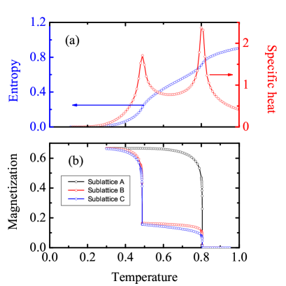
Figure 20: (Color online) Thermodynamic properties of the $q=3$ Potts model on the isotropic centered diced lattice. (a) Entropy and specific heat obtained by iTEBD with $D=40$. (b) Magnetizations of the A, B, and C sublattices obtained by iTEBD with $D=30$.

We summarize this section by stating that we have explored a number of models in which partial order emerges as a phase intermediate between a low-temperature phase of complete order and a high-temperature phase of complete disorder. In principle one may also expect that this is not a requirement, in that a sufficiently complex model may contain more than one type of partially ordered phase, including a partially ordered ground state, and in this case it would be possible to investigate further types of sequential phase transition to states of different intermediate partial order. However, these phases do not emerge from within the confines of the geometries (Archimedean and Laves lattices only) and coupling constants (mostly isotropic) we consider. The emergence of intermediate partial order is neither a consequence of frustration (Sec. VIA only) nor of anisotropic couplings (see Sec. VIC), the difference between the $q=3$ Union-Jack and centered diced lattices being a result of their connectivity. Quite generally, a Potts model possesses a number of symmetries, which depend on both the geometry of the lattice and on the Potts degeneracy $q$, and these may be broken partially and sequentially at the different transitions from full to partial to no order.

VII Partial Order with Sub-Extensive Residual Entropy

We conclude our investigation of the different types of partial order in AF Potts models by considering the form of the configurational entropy. In all of the models studied in the preceding sections, the partially ordered ground and intermediate states always possess an extensive degeneracy and thus a non-zero entropy per site. In this section, we discuss the issue of partial order in the ground states of systems whose entropy is sub-extensive, such that the residual (zero-temperature) entropy per site is $0$.

VII.1 Generalized Decorated Square Lattice

We introduced the concept of partial order arising from sub-extensive residual entropy in a study gdsl of the AF Potts model on the generalized decorated square lattice, particularly the $q=3$ case, and summarize the results in this subsection. The Union-Jack lattice is obtained from the square lattice by adding one site at the center of each square; if centering sites are placed only on alternate squares, or equivalently the Union-Jack lattice is alternately diluted, one obtains the generalized decorated square lattice shown in Fig. 21(a), with two different couplings $J_{1}$ and $J_{2}$. Like the Union-Jack lattice, this lattice is tripartite (three-colorable in graph theory), but because the lattice is formed of both triangular and square polygons, the division into three sublattices is not unique.

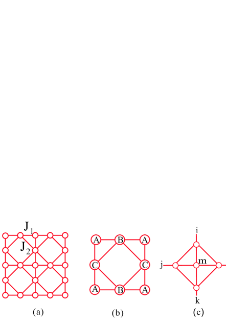
Figure 21: (Color online) (a) Generalized decorated square lattice. (b) For the sublattice partition illustrated, sites in sublattices B and C have coordination numbers $z_{B}=z_{C}=6$ and those in sublattice A have $z_{A}=4$. (c) Definition of tensors in each unit cell of the lattice.

The local tensor for the generalized decorated square lattice is given by

$$T_{ijkl}= \sum\limits_{m}\!\exp[-\beta J_{1}(\delta_{\sigma_{i},\sigma_{m}}\!\!+\!\delta_{\sigma_{j},\sigma_{m}}\!\!+\!\delta_{\sigma_{k},\sigma_{m}}\!\!+\!\delta_{\sigma_{l},\sigma_{m}})]$$ (29)

$$\;\times\;\exp[-\beta J_{2}(\delta_{\sigma_{i},\sigma_{j}}\!\!+\!\delta_{\sigma_{j},\sigma_{k}}\!\!+\!\delta_{\sigma_{k},\sigma_{l}}\!\!+\!\delta_{\sigma_{l},\sigma_{i}})]$$

and represented in Fig. 21(c). The Potts variables $\sigma_{i}$ on each site serve as the indices of the tensors, and the tensors for each unit cell may be combined to form a square-lattice tensor network. Because the partition of the lattice into three sublattices is not unique, the ground state of the AF $q=3$ Potts model is not expected to be as straightforward as the (zero-entropy) three-sublattice order of the same model on the triangular, Union-Jack, or centered diced lattices. Indeed, the specific heat shown in Fig. 22 for the case $J_{1}=J_{2}=1$ appears to lack any evidence of a phase transition. However, on careful inspection it reveals not a divergence but a small discontinuity qualitatively similar to that of the $q=4$ Union-Jack lattice (Sec. IVB), which marks a phase transition to partial order at $T_{c}=0.5373(1)$ (detected more clearly but less accurately through the magnetization and the susceptibility shown in Ref. gdsl ).

To understand the origin of this behavior, we considered gdsl the configurations minimizing the bond energy that make up the ground manifold. Sites in a single sublattice are expected to order ferromagnetically because they are separated by pairs of AF bonds. If the B sublattice in Fig. 21(b) is ordered with $\sigma_{i}=0$, the state on the intervening lines of A and C sites may be either $121212\dots 12$ or $212121\dots 21$, each with probability 50%. An analogous state exists for order only on the C sublattice, but the two are mutually exclusive; both ordered states break the $\pi/2$ rotation symmetry of the lattice (also broken on the Union-Jack lattice for $q=4$, where a similar competition between ordered states causes the weak transition in $C(T)$). It is the linear structures of alternating order that hold the key to the properties of the system. If one calculates the degeneracy of the ground manifold for a system of size $L\times L$, it is ${\cal S}=6(2^{L}-1)$, a quantity exponential only in the linear size of the system and not in its volume. Thus the residual entropy per site is

$$S_{0}=\lim_{L\rightarrow\infty}\frac{\log(6\times 2^{L}-6)}{L^{2}}=0,$$ (30)

vanishing due to the one-dimensional nature of the ground-state degrees of freedom. However, the selection of a partially ordered ground state within this model, proceeding in the same way as the extensively degenerate examples studied in Sec. IV, indicates that a large but sub-extensive degeneracy of Potts configurations is sufficient to drive this phenomenon.

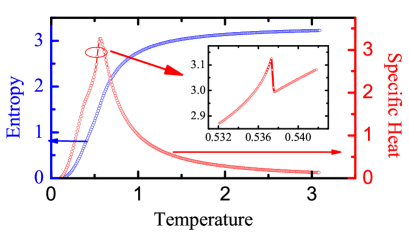
Figure 22: (Color online) Specific heat for the $q=3$ AF Potts model on the generalized decorated square lattice with $J_{1}=J_{2}=1$. The results are obtained by iTEBD with $D=30$. The inset shows the very narrow discontinuity appearing at $T_{c}=0.5373(1)$.

VII.2 Dilute Centered Diced Lattices

We continue by demonstrating that partial order with sub-extensive entropy can occur more generally than in a single lattice. In the same way that partial dilution of the centering sites of the Union-Jack lattice leads to the generalized decorated square lattice, dilution of the centering sites of the centered diced lattice leads to a further class of irregular lattices. The centering sites of the centered diced lattice form a kagome lattice (yellow sites in Fig. 10), which is a tripartite geometry offering many ways to divide all the sites into three disconnected sublattices; the two most common are known as the $k=0$ and $\sqrt{3}\times\sqrt{3}$ structures rc .

We consider only commensurate dilutions yielding small unit cells, which leaves two choices of dilution, namely 1/3 and 2/3. If $2/3$ of the centering sites are removed, such that only one sublattice of the kagome lattice has a Potts variable and the other two sublattices are empty, we obtain the lattices shown in Fig. 23 as IA and IB. If 1/3 of the centering sites are removed, leaving a regular 2/3 filling, we obtain the lattices IIA and IIB. We note that lattices IB and IIB contain the additional complexity of inequivalent A sites (specifically, in lattice IB these have coordinations 6 and 9, while in IIB they have 9 and 12) and we do not consider these geometries further; this is equivalent to considering only the $k=0$ structures (IA and IIA). If the sublattices A and B of the diced lattice are labeled as in Sec. IVC, and the remaining centering sites form a partial sublattice C, then lattice IA has site numbers $N_{A}=N/4$, $N_{B}=N/2$, and $N_{C}=N/4$, with respective coordination numbers $z_{A}=8$ and $z_{B}=z_{C}=4$, while lattice IIA has $N_{A}=N/5$ and $N_{B}=N_{C}=2N/5$ with $z_{A}=10$, $z_{B}=5$, and $z_{C}=4$.

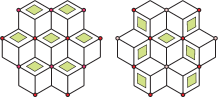
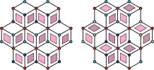
IA       IB       IIA       IIB

Figure 23: (Color online) Dilute centered diced lattices. The quadrilaterals containing centering sites are marked in color. In lattices IA and IB, $1/3$ of the quadrilaterals have center sites, while lattices IIA and IIB have center sites on $2/3$ of the quadrilaterals. Lattices IA and IIA correspond to $k=0$ arrangements on the kagome lattice formed by all of the centering sites in the centered diced lattice, whereas lattices IB and IIB are $\sqrt{3}\times\sqrt{3}$ arrangements.

VII.2.1 IIA Lattice

We begin by considering the IIA lattice with $q=3$. For every centered rhombus, every bond can be satisfied if both pairs of diagonal sites have the same $\sigma_{i}$. Thus all A sites are mutually ferromagnetic, by convention with $\sigma_{A}=0$, and all B sites between two horizontal lines of A sites (Fig. 23, IIA) should also have the same $\sigma_{B}\neq 0$, but the values of $\sigma_{B}$ on the different (horizontal, zig-zag) lines of B sites are independent, i.e. $\sigma_{B}=1$ or 2 at random. The value of $\sigma_{C}$ is fixed for all C sites once $\sigma_{A}$ and the lines of $\sigma_{B}$ values are known. Thus the ground-state degeneracy is $2^{L}$, where $L=\sqrt{N_{A}}$ is the number of lines of A sites. As a consequence, the residual entropy per site in the thermodynamic limit is $0$ for the same reason, linear structure formation, as in the $q=3$ model on the generalized decorated square lattice (Sec. VIIA).

Figure 24 shows the entropy, specific heat, and magnetization of sublattice A for the IIA dilute centered diced lattice. The zero-temperature entropy per site is $0$, in accord with the analysis above. The peak in the specific heat indicates that a finite-temperature phase transition occurs at $T_{c}=0.74(1)$. The magnetization of the A sublattice is $2/3=1-1/3$, corresponding to perfect order, while the analogous quantities for the B and C sublattices (not shown) exhibit perfect disorder. Thus the IIA lattice provides another example of partial order in the ground state selected by a sub-extensive residual entropy.

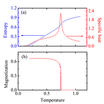
Figure 24: (Color online) Thermodynamic properties of the $q=3$ Potts model on the IIA lattice of Fig. 23. The results are obtained by iTEBD with $D=40$. (a) Entropy and specific heat. (b) Magnetization of the A sublattice.

By contrast, despite the linear structure of the lattice, the $q=4$ model in the same geometry shows very different behavior. In Ref. gdsl we demonstrated that the AF $q=4$ Potts model on the generalized decorated square lattice is critical at zero temperature, its susceptibility approaching a divergence as $T\rightarrow 0$. However, on the IIA lattice with $q=4$ we find a “conventional” finite-temperature phase transition at $T_{c}=0.48(1)$, appearing as a clear peak in the specific heat in Fig. 25(a) and with a large residual entropy per site, $S_{{\rm IIA},q=4}(0)=0.5556$. Straightforward counting arguments for perfect partial order only on the A, B, or C sublattices reveal respective ground-state degeneracies $g_{A}=2^{4N/5}(3/2)^{L}$, $g_{B}=\exp(3NS_{{\rm ds},q=3}(0)/5)]$, where $S_{{\rm ds},q=3}(0)=0.561070$ is the residual entropy for the $q=3$ decorated square lattice (Sec. IVB), and $g_{C}=1.606^{3N/5}$, where the numerical properties are given by the $q=3$ diced lattice of the A and B sites. Clearly a partial order on the A sublattice remains the most favorable, and indeed our computed entropy is very close to the value $S_{A}=(4/5)\ln 2=0.5545$ obtained in this case. The zero-temperature A-sublattice magnetization is $M_{{\rm IIA},q=4}^{A}=0.7438$ [Fig. 25(b)], a result within 0.8% of the the ideal value $0.75=1-1/4$. The discrepancies of both entropy and magnetization from their ideal values indicate the presence of non-negligible contributions from different ground-state configurations, but no changes to the qualitative physics of Sec. IV.

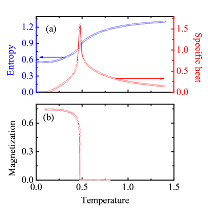
Figure 25: (Color online) Thermodynamic properties of the $q=4$ Potts model on the IIA lattice of Fig. 23. The results are obtained by iTEBD with $D=40$. (a) Entropy and specific heat. (b) Magnetization of the A sublattice.

VII.2.2 IA Lattice

For completeness, we conclude by considering the IA dilute centered diced lattice of Fig. 23. Because this geometry also consists of linear structures in two dimensions, it is not unreasonable to expect a further example of partial order with sub-extensive residual entropy. As noted above, every centered rhombus in an AF Potts model with $q=3$ has the same $\sigma_{i}$ for diagonal pairs of sites, and thus all A sites in the same horizontal line have the same state, but the A sites on adjacent lines may take the same or different states $\sigma_{i}$ with complete energetic degeneracy. For fully ferromagnetic A sites, for example with $\sigma_{i}=0$, pairs of B sites in every centered rhombus retain two independent choices, $\sigma_{i}=1$ or 2, and the degeneracy is $2^{N/4}$ ($N/4$ is the number of centered rhombi). However, if there exists a row of A sites with $\sigma_{i}=1$, then the B sites in this row and both its neighboring rows become fixed to $\sigma_{i}=2$ and the degeneracy falls to $2^{N/4-3L}$, where $L=\sqrt{N/4}$ is the number of centered rhombi in a row. Thus configurations in which all A sites have the same value are dominant in the ground state but one expects a finite residual entropy of $S_{{\rm IA},q=3}^{A}(0)=(1/4)\ln 2=0.173286795139986$.

In Fig. 26, we present the entropy, specific heat, and the A-sublattice magnetization of the AF $q=3$ Potts model on the IA lattice. Our numerical result for the zero-temperature entropy, $S_{{\rm IA},q=3}(0)=0.17328679513999$ confirms completely the analytical reasoning. Both the specific heat and the sublattice magnetization confirm a conventional entropy-driven phase transition at $T_{c}=0.66(1)$ and the magnetization of the A sublattice in the low-temperature limit is the expected $2/3=1-1/3$. We conclude that linear structures may be a necessary but not a sufficient condition for partial order from sub-extensive residual entropies in two dimensions, but that the fundamental criterion for partial order, namely the relationship between ${\bar{z}}$ and $q$, remains the dominant determining factor.

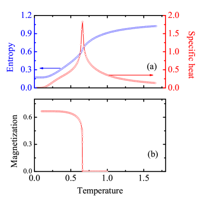
Figure 26: (Color online) Thermodynamic properties of the $q=3$ Potts model on the IA lattice of Fig. 23. The results are obtained by iTEBD with $D=40$. (a) Entropy and specific heat. (b) Magnetization of the A sublattice.

We end with the $q=4$ model on the IA lattice. In this case the degeneracy is large and the connectivity smaller than the IIA lattice, so one may even suspect a zero-temperature critical phase with no true order gdsl . Focusing directly on a candidate partially ordered state with all A sites ferromagnetic ($\sigma_{A}=0$), the Potts variables on the B and C sites in each centered rhombus are independent. If the C sites have $\sigma=1$, the two B sites can be $(2,2)$, $(2,3)$, $(3,2)$, or $(3,3)$, and so the centered rhombus has $3\times 4=12$ configurations, giving a total degeneracy $g_{A}=12^{N/4}$. The analogous degeneracies for full B- and C-sublattice order are $g_{B}=2^{N/2}(3/2)^{L}$ and $g_{C}=1.606^{3N/4}$, confirming that if a partially ordered state exists then it will be on the A sublattice.

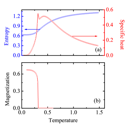
Figure 27: (Color online) Thermodynamic properties of the $q=4$ Potts model on the IA lattice of Fig. 23. The results are obtained by iTEBD with $D=40$. (a) Entropy and specific heat. (b) Magnetization of the A sublattice.

The entropy, specific heat, and A sublattice magnetization of the $q=4$ AF Potts model on the IA lattice are shown in Fig. 27. A finite-temperature phase transition does in fact occur, at $T_{c}=0.32(1)$. However, the associated discontinuity is not the dominant feature in the specific heat, a situation more reminiscent of the $q=4$ model on the Union-Jack lattice (Sec. IVB) and the $q=3$ model on the generalized decorated square lattice (Sec. VIIA), and the transition temperature is one of the lowest finite values we have encountered. The evidence for a general lack of robustness to thermal fluctuations in this model is reinforced by our results for the residual entropy, $S_{{\rm IA},q=4}(0)=0.63402$, which lies above the perfect-order value $(1/4)\ln 12=0.6212$ by an amount we have seen (Sec. IV) to be significant. Similarly, although our results confirm that the partial order is on the A sublattice, the zero-temperature magnetization $M_{{\rm IA},q=4}(0)=0.6725$ lies well below the ideal value of 0.75.

VIII Summary

We have performed a detailed analysis of the antiferromagnetic Potts model in two dimensions, covering a range of lattice geometries and numbers $q$ of degrees of freedom per site. The primary focus of our investigation is the phenomenon of partial long-range order, which arises in the presence of high state degeneracies. Quite generally, this partial order sets in at a “finite-temperature phase transition,” which is the defining property of the Potts model in question, but whose properties can differ widely as a consequence of the interplay between lattice geometry and $q$ value.

An essential ingredient of the partial ordering scenario is the nature of the lattice. In the absence of frustration, ordering transitions occur when the site coordination number $z$ constrains the number of degrees of freedom $q$. For sufficiently large $q$, the AF Potts model on any lattice is insufficiently constrained and is disordered at all temperatures. In restricting our considerations to Archimedean and Laves lattices, one of the key qualitative properties of a lattice is whether it is regular (all sites equivalent) or irregular, meaning that it has different types of site with different local coordination numbers. While both types of system may possess a large number of Potts configurations minimizing the total energy, the irregular lattices have nontrivial entropies, which in a number of cases drive only a partial ordering transition on some of the inequivalent sublattices.

The majority of our results are obtained for three particular Laves lattices, the diced, Union-Jack, and centered diced lattices, which have integer average coordination number ${\bar{z}}$ but behavior rather different from regular lattices with $z={\bar{z}}$. Specifically, for the value $q=q_{c}$ where the regular lattice is critical, they all show finite-temperature transitions to states of partial order. Thus the irregular lattice geometry leads quite generally to high values of $q_{c}$ (indeed, $q_{c}>5$ for ${\bar{z}}=6$ on the centered diced lattice). The entropic selection mechanism is such that the partial order is always on the site of highest local coordination, which creates a high number of satisfied bonds while imposing a $q-1$ Potts degeneracy on all of the connected sites.

The finite-temperature transitions from partially ordered states to disordered states may in different cases be very obvious or extremely subtle. We have analyzed both types and shown that this is a function of the number of competing partially ordered states; when there is no unique sublattice with the largest connectivity, then the system must resolve this competition and the result can be a very weak transition. Indeed, the existence of inequivalent sites in a lattice cannot on its own guarantee a partially ordered ground state, because sufficiently large $q$ will always cause disorder, and so the existence of order must be tested in every case. However, the effectiveness of thermal fluctuations in suppressing the partial order parameter is determined not only by the number of degenerate states in the manifold but also by the nature of the competition between partially ordered states.

Another factor in this competition can be the nature of the entropic driving forces. In most of the models we have studied, the entropy of the ground manifold of minimum-energy states is extensive, scaling with the volume of the system. However, we have also discovered some situations where the balance of connectivity (${\bar{z}}$), $q$, and the interactions ($J$) is such that the ground state has one-dimensional correlations and the degeneracy scales only with the linear dimension of the system. Despite the resulting sub-extensive entropy, the ground manifold remains highly degenerate, and this is sufficient to preserve the physics of partial order.

We comment here that we have largely avoided considering systems with frustrated interactions. Frustration is regarded as a very general driving force for (complete) suppression of order parameters and in certain systems for the existence of only partially ordered ground states. The family of AF Potts models can largely be categorized into three regimes, one with $q>{\bar{z}}$, which exhibits disorder at all temperatures, one with (crudely) $q\sim{\bar{z}}$, which exhibits phenomena including zero-temperature criticality and entropy-driven partial order, and one with $q\ll{\bar{z}}$ where the ground state usually has complete order. Frustration is the key factor affecting the nature and extent of order in the last of these categories. This paper concerns almost exclusively the intermediate category, where entropic effects dominate and frustration is absent – quite simply, a triangle is not a frustrated unit when $q\geq 3$.

In addition to partially ordered ground states, we have also investigated the formation of partially ordered states at intermediate temperatures. In the models we consider, these occur in systems with conventional, fully ordered ground states, which are also states of low (or zero) degeneracy. As the temperature is increased, the huge entropic preference for partially ordered states of high degeneracy can drive an additional phase transition. The typical regime for this type of behavior is where $q$ is slightly smaller than in the systems with partially ordered ground states. The consequence is a system with multiple phase transitions, from order to partial order at low temperatures and then from partial order to complete disorder, which we are able to characterize completely by computing the magnetizations on every sublattice. Potts models possess both the symmetry of their lattice and the $q$-fold permutation symmetry of the Potts variable, and models showing separate phase transitions give a very clear example of sequential breaking or restoration of partial symmetries, which can be used to classify the transition type (universality class)Wu1982_RMP54-235 .

One of the key features of our calculations is that they yield quantitative thermodynamic information about Potts models, and in particular about the partially ordered states at low temperatures. Highly accurate values for the entropies and magnetizations can be compared with expectations for different, competing, partially ordered model states, to deduce their contributions to the true ground state. In this study, we have exposed a number of models where the thermodynamic properties do not match with naive expectations based on perfect order on the highest-coordinated sublattice. For reasons of space, we have not dwelled on the development of scenarios for improving the analytical description of Potts states, although our data allow direct comparisons with models for the leading “defect” configurations within a state of perfect partial order. When these defects are present at finite densities due to their entropic contributions, their effects will be observable in the entropy and sublattice magnetization we compute. Our results also permit detailed comparisons with different models in classical statistical mechanics, further developing cross-links within the field.

Finally, we have demonstrated the power of tensor-based numerical methods for problems in classical statistical mechanics. The ability to express the partition function as a tensor product, to renormalize systematically, and to truncate in the tensor dimension, gives unprecedented access to accurate thermodynamic information. The method is completely general in that calculations can be performed for all lattice geometries and all values of $q$, with no restrictions to special cases. We have exploited this power to find and characterize previously unknown phase transitions, to quantify thermodynamic properties both at the transition and at low temperatures, and thus to gain extra insight into the physics of partial ordering processes. We close by noting that the development of tensor-based numerical techniques remains in its relative infancy, and that significant improvements in size (tensor dimension) and accuracy may still be expected. This would make possible a new level of quantitative discussion for topics such as scaling exponents and universality at phase transitions, which are currently still at the frontiers of our capabilities.

- (1) F. Y. Wu, Rev. Mod. Phys. 54, 235 (1982).
- (2) R. B. Potts, Ph.D. thesis, University of Oxford (1951).
- (3) Phase Transitions and Critical Phenomena Vol 1, edited by C. Domb and M. S. Green (Academic Press, London and New York, 1972).
- (4) L. Onsager, Phys. Rev. 65, 117 (1944).
- (5) G. H. Wannier, Phys. Rev. 79, 357 (1950).
- (6) R. J. Baxter, S. B. Kelland, and F. Y. Wu, J. Phys. A: Math. Gen. 9, 397 (1976).
- (7) R. J. Baxter, J. Math. Phys. 11, 784 (1970).
- (8) J. L. Jacobsen, J. Phys. A: Math. Theor. 32, 5445 (1999).
- (9) J. Salas and A. D. Sokal, J. Stat. Phys. 86, 551 (1997).
- (10) J. Salas and A. D. Sokal, J. Stat. Phys. 92, 729 (1998).
- (11) D. A. Huse and A. D. Rutenberg, Phys. Rev. B 45, 7536 (1992).
- (12) C. Moore and M. E. J. Newman, J. Stat. Phys. 99, 629 (2000).
- (13) N. G. Parsonage and L. A. K. Staveley, Disorder in Crystals (Oxford University Press, New York, 1978).
- (14) R. Kotecky, J. Salas, and A. D. Sokal, Phys. Rev. Lett. 101, 030601 (2008).
- (15) L. Pauling, J. Am. Chem. Soc. 57, 2680 (1935).
- (16) A. Lipowski, T. Horiguchi, and Y. Honda, Physica A 237, 297 (1997).
- (17) Q. N. Chen, M. P. Qin, J. Chen, Z. C. Wei, H. H. Zhao, B. Normand, and T. Xiang, Phys. Rev. Lett. 107, 165701 (2011).
- (18) O. Nagai, S. Miyashita, and T. Horiguchi, Phys. Rev. B 47, 202 (1993).
- (19) V. G. Vaks, A. I. Larkin, and Y. N. Ovchinnikov, JETP Letters. 22, 820 (1966).
- (20) P. Azaria, H. T. Diep, and H. Giacomini, Phys. Rev. Lett. 59, 1629 (1987).
- (21) M. Debauche and H. T. Diep, Phys. Rev. B 46, 8214 (1992).
- (22) H. T. Diep, M. Debauche, and H. Giacomini, Phys. Rev. B 43, 8759 (1991).
- (23) G. Andre, R. Bidaux, J.-P. Carton, and L. de Seze, J. Phys. (France) 40, 479 (1979).
- (24) D. P. Foster, C. Gerard, and I. Puha, J. Phys. A: Math. Gen. 34, 5183 (2001).
- (25) D. P. Foster and C. Gerard, Phys. Rev. B 70, 014411 (2004).
- (26) D. Blankschtein, M. Ma, A. N. Berker, G. S. Grest, and C. M. Soukoulis, Phys. Rev. B 29, 5250 (1984).
- (27) P. Azaria, H. T. Diep, and H. Giacomini, Europhys. Lett. 9, 755 (1989).
- (28) C. Santamaria and H. T. Diep, J. Appl. Phys. 81, 5276 (1997).
- (29) D. Blankschtein, M. Ma, and A. N. Berker, Phys. Rev. B 30, 1362 (1984).
- (30) H. T. Diep, P. Lallemand, and O. Nagai, J. Phys. C: Solid State Phys. 18, 1067 (1985).
- (31) R. Igarashi and M. Ogata, J. Phys: Conf. Ser. 200, 022019 (2010).
- (32) E. H. Boubcheur, R. Quartu, H. T. Diep, and O. Nagai, Phys. Rev. B 58, 400 (1998).
- (33) J. R. Stewart, G. Ehlers, A. S. Wills, S. T. Bramwell, and J. S. Gardner, J. Phys.: Condens. Matter 16, L321 (2004).
- (34) S. Hayami, M. Udagawa, and Y. Motome, J. Phys. Soc. Jpn. 80, 073704 (2011).
- (35) S. Hayami, M. Udagawa, and Y. Motome, J. Phys: Conf. Ser. 400, 032018 (2012).
- (36) R. Quartu and H. T. Diep, Phys. Rev. B 55, 2975 (1997).
- (37) C. Santamaria, R. Quartu, and H. T. Diep, J. Appl. Phys. 84, 1953 (1998).
- (38) J. S. Wang, R. H. Swendsen, and R. Kotecky, Phys. Rev. Lett. 63, 109 (1989).
- (39) J. S. Wang, R. H. Swendsen, and R. Kotecky, Phys. Rev. B 42, 2465 (1990).
- (40) J. Salas and A. D. Sokal, J. Stat. Phys. 144, 1028 (2011).
- (41) J. L. Jacobsen and C. R. Scullard, J. Phys. A: Math. Theor. 46, 075001 (2013).
- (42) Q. N. Chen, Ph.D. thesis, Institute of Theoretical Physics, Chinese Academy of Sciences, China (2012).
- (43) R. J. Baxter, J. Phys. C: Solid State Phys. 6, L445 (1973).
- (44) A. Bazavov, B. A. Berg, and S. Dubey, Nucl. Phys. B 802, 421 (2008).
- (45) S. Wang, Z. Y. Xie, J. Chen, B. Normand, and T. Xiang, Chin. Phys. Lett. 31, 070503 (2014).
- (46) P. L. Dobruschin, Theory Probab. Appl. 13, 197 (1968).
- (47) P. L. Dobruschin, Theory Probab. Appl. 15, 458 (1970).
- (48) M. P. M. den Nijs, M. P. Nightingale, and M. Schick, Phys. Rev. B 26, 2490 (1982).
- (49) J. Salas, J. Phys. A: Math. Gen. 31, 5969 (1998).
- (50) Y. Matsuda, Y. Kasai, and I. Syozi, Prog. Theor. Phys. 65, 1091 (1981).
- (51) M. P. Qin, J. Chen, Q. N. Chen, Z. Y. Xie, X. Kong, H. H. Zhao, B. Normand, and T. Xiang, Chin. Phys. Lett. 30, 076402 (2013).
- (52) K. Appel and W. Haken, Illinois J. Math. 21, 429 (1977).
- (53) K. Appel, W. Haken, and J. Koch, Illinois J. Math. 21, 491 (1977).
- (54) F. Verstraete, V. Murg, and J. I. Cirac, Adv. Phys. 57, 143 (2008).
- (55) V. Murg, F. Verstraete, and J. I. Cirac, Phys. Rev. Lett. 95, 057206 (2005).
- (56) H. C. Jiang, Z. Y. Weng, and T. Xiang, Phys. Rev. Lett. 101, 090603 (2008).
- (57) Z. Y. Xie, H. C. Jiang, Q. N. Chen, Z. Y. Weng, and T. Xiang, Phys. Rev. Lett. 103, 160601 (2009).
- (58) H. H. Zhao, Z. Y. Xie, Q. N. Chen, Z. C. Wei, J. W. Cai, and T. Xiang, Phys. Rev. B 81, 174411 (2010).
- (59) H. H. Zhao, Cenke Xu, Q. N. Chen, Z. C. Wei, M. P. Qin, G. M. Zhang, and T. Xiang, Phys. Rev. B 85, 134416 (2012).
- (60) Z. Y. Xie, J. Chen, J. F. Yu, X. Kong, B. Normand, and T. Xiang, Phys. Rev. X 4, 011025 (2014).
- (61) J. Jordan, R. Orus, and G. Vidal, Phys. Rev. B 79, 174515 (2009).
- (62) T. Barthel, C. Pineda, and J. Eisert, Phys. Rev. A 80, 042333 (2009).
- (63) C. V. Kraus, N. Schuch, F. Verstraete, and J. I. Cirac, Phys. Rev. A 81, 052338 (2010).
- (64) G. Vidal, Phys. Rev. Lett. 99, 220405 (2007).
- (65) Z. C. Gu, M. Levin, and X.-G. Wen, Phys. Rev. B 78, 205116 (2008).
- (66) A. W. Sandvik and G. Vidal, Phys. Rev. Lett. 99, 220602 (2007).
- (67) J. F. Yu, Z. Y. Xie, Y. Meurice, Yuzhi Liu, A. Denbleyker, Haiyuan Zou, M. P. Qin, J. Chen, and T. Xiang, Phys. Rev. E 89, 013308 (2014).
- (68) M. Levin and C. P. Nave, Phys. Rev. Lett. 99, 120601 (2007).
- (69) G. Vidal, Phys. Rev. Lett. 98, 070201 (2007).
- (70) R. Orus and G. Vidal, Phys. Rev. B 78, 155117 (2008).
- (71) R. Orus and G. Vidal, Phys. Rev. B 80, 094403 (2009).
- (72) R. Orus, Phys. Rev. B 85, 205117 (2012).
- (73) L. Wang, Y. J. Kao, and A. W. Sandvik, Phys. Rev. E 83, 056703 (2011).
- (74) Z. Y. Xie, J. Chen, M. P. Qin, J. W. Zhu, L. P. Yang, and T. Xiang, Phys. Rev. B 86, 045139 (2012).
- (75) D. Perez-Garcia, F. Verstraete, M. M. Wolf, and J. I. Cirac, Quantum Inf. Comput. 7, 401 (2007).
- (76) J. O. Fjaerestad, J. Stat. Mech. P01004 (2010).
- (77) Y. J. Deng, Y. Huang, J. L. Jacobsen, J. Salas, and A. D. Sokal, Phys. Rev. Lett. 107, 150601 (2011).
- (78) E. H. Fradkin and T. P. Eggarter, Phys. Rev. A 14, 495 (1976).
- (79) A. Chubukov, Phys. Rev. Lett. 69, 832 (1992).