Lecture notes on
“Quantum chromodynamics and statistical physics”

Abstract

The concepts and methods used for the study of disordered systems have proven useful in the analysis of the evolution equations of quantum chromodynamics in the high-energy regime: Indeed, parton branching in the semi-classical approximation relevant at high energies is a peculiar branching-diffusion process, and parton branching supplemented by saturation effects (such as gluon recombination) is a reaction-diffusion process. In these lectures, we first introduce the basic concepts in the context of simple toy models, we study the properties of the latter, and show how the results obtained for the simple models may be taken over to quantum chromodynamics.

1 Branching random walks and the Fisher-Kolmogorov-Petrovsky-Piscounov equation

In this section, we shall introduce branching random walks, which are a class of stochastic processes appearing in many different branches of science, and in particular in particle physics. We show how a nonlinear diffusion equation called the FKPP equation characterizes some properties of the realizations of branching random walks. We start by recalling some elementary facts on ordinary Brownian motion, before adding in the branching process.

1.1 Brownian motion

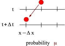
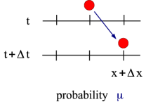
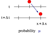
Consider a one-dimensional lattice indexed by the variable $x$, with lattice spacing $\Delta x$. We start with a single particle at site 0. We take the following rule for the evolution of the system from time $t$ to time $t+\Delta t$, which consists in two elementary processes: The particle has the probability $\mu$ to jump on the lattice site to the left, and the probability $\mu$ to jump to the right. Hence by probability conservation, the particle has the probability $1-2\mu$ to stay at its current position (from which we see that $\mu$ has to be chosen less than $\frac{1}{2}$).

Figure 1: Definition of the elementary processes and illustration of one step of the Brownian motion on the lattice. The particle sits at position $x$ at time $t$. According to the evolution rules, it may jump left with probability $\mu$, right also with probability $\mu$, and it may stay at $x$ with probability $1-2\mu$. In the particular realization shown in the figure, the particle jumps right, in such a way that its position be $x+\Delta x$ at time $t+\Delta t$.

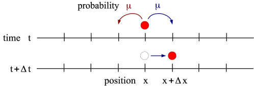
With this rule, it is straightforward to establish an equation for the probability $P(x,t)$ that the particle be on site $x$ at time $t$: We simply relate $P$ at time $t+\Delta t$ to $P$ at time $t$ with the help of the probabilities of the elementary processes. The different terms which contribute to $P(x,t+\Delta t)$ stem from the following cases:

1. The particle is at site $x-\Delta x$ at time $t$ and makes a right jump. This generates the term $P(x-\Delta x,t)\times\mu$;

2. the particle is at $x+\Delta x$ at $t$ and makes a left jump. The corresponding term reads $P(x+\Delta x,t)\times\mu$;

3. the particle is already at $x$ at time $t$ and does not move. The term which describes this case is $P(x,t)\times(1-2\mu)$.

Summing all contributions, one arrives at

$$P(x,t+\Delta t)=P(x-\Delta x,t)\mu+P(x+\Delta x,t)\mu+P(x,t)(1-2\mu)$$ (1)

from which, after a trivial rearrangement, we get the finite difference evolution equation

$$P(x,t+\Delta t)-P(x,t)=\mu\left[P(x-\Delta x,t)+P(x+\Delta x,t)-2P(x,t)\right].$$ (2)

It is often easier to deal analytically with differential equations rather than difference equations. If we let the lattice spacing $\Delta x$ and the time step $\Delta t$ go to zero, the above finite-difference equation becomes a partial differential equation. We must be careful however to keep the ratio

$$D\equiv\mu\frac{(\Delta x)^{2}}{\Delta t}$$ (3)

finite and fixed when taking this limit in such a way that no relevant terms in Eq. (2) vanish. We get

$$\frac{\partial P}{\partial t}=D\frac{\partial^{2}P}{\partial x^{2}}.$$ (4)

This equation is the so-called Fokker-Planck equation for our process, and we recognize that it is the simple diffusion equation. To set up a well-posed problem, we need to specify the initial condition and the boundary conditions. The initial condition is a single particle at site $x=0$ at time $t=0$, hence in the continuous limit

$$P(x,t=0)=\delta(x).$$ (5)

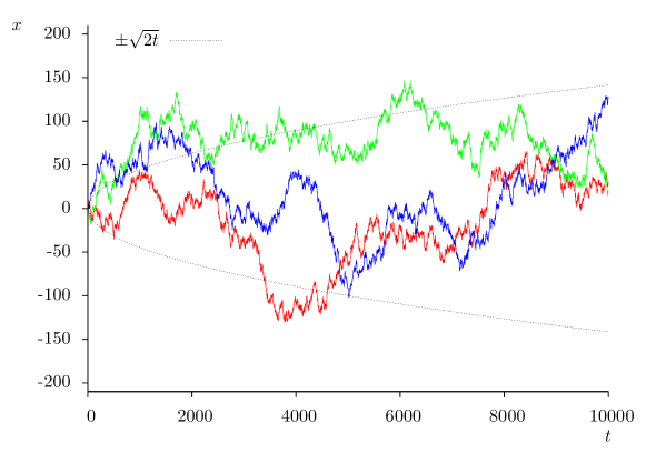
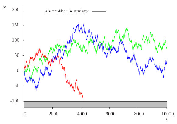
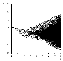
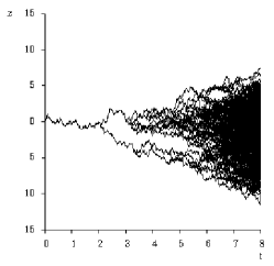
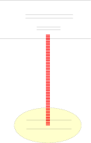
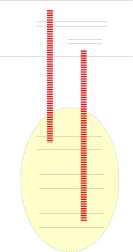
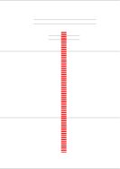
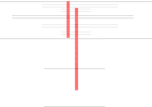
As for the boundary conditions, we shall first opt for free ones, and second impose a fixed absorptive boundary. In the following, we shall set $D=1$ for simplicity. (From dimensional analysis, one may always re-establish a general diffusion constant). Realizations of this model are shown in Fig. 2.

Figure 2: Three realizations of the continuous Brownian up to $t=10000$. The parabola (dotted lines) represents the standard deviation $\pm\sqrt{\langle x^{2}\rangle-\langle x\rangle^{2}}$.

First, we choose free boundary conditions. A general solution to Eq. (4) is easily obtained as a superposition of exponentials,

$$P(x,t)=\int_{\gamma_{0}-i\infty}^{\gamma_{0}+i\infty}\frac{d\gamma}{2i\pi}e^{-\gamma x}\tilde{P}(\gamma,t).$$ (6)

From Eq. (4), $\tilde{P}$ obeys the ordinary first-order differential equation

$$\frac{d\tilde{P}(\gamma,t)}{dt}=\gamma^{2}\tilde{P}(\gamma,t),$$ (7)

with the initial condition $\tilde{P}(\gamma,t=0)=1$. The solution is trivial:

$$\tilde{P}(\gamma,t)=e^{\gamma^{2}t}.$$ (8)

One then inserts this expression in Eq. (6) in order to compute $P(x,t)$:

$$P(x,t)=\int_{\gamma_{0}-i\infty}^{\gamma_{0}+i\infty}\frac{d\gamma}{2i\pi}e^{-\gamma x+\gamma^{2}t}=e^{-\frac{x^{2}}{4t}}\int_{\gamma_{0}-i\infty}^{\gamma_{0}+i\infty}\frac{d\gamma}{2i\pi}e^{t\left(\gamma-\frac{x}{2t}\right)^{2}}.$$ (9)

Performing the change of variable $\gamma=\frac{x}{2t}+i\frac{\nu}{\sqrt{t}}$ and sliding the integration contour in such a way that $\gamma_{0}=\frac{x}{2t}$, we are left with a standard Gaussian integral

$$P(x,t)=\frac{e^{-\frac{x^{2}}{4t}}}{\sqrt{t}}\int_{-\infty}^{+\infty}\frac{d\nu}{2\pi}e^{-\nu^{2}}.$$ (10)

Finally,

$$P(x,t)=\frac{1}{\sqrt{4\pi t}}e^{-\frac{x^{2}}{4t}}.$$ (11)

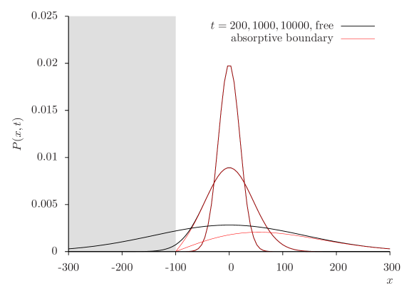
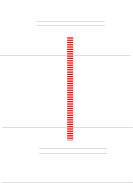
This function (of $x$) is represented in Fig. 4 (at different times $t$).

In order to characterize such a probability distribution, it is useful to introduce the generating function of its moments:

$$G(\lambda,t)=\left\langle e^{\lambda x}\right\rangle\equiv\int_{-\infty}^{+\infty}dx\,P(x,t)\,e^{\lambda x},$$ (12)

whose expansion in powers of $\lambda$ has the moments of $x$ as coefficients:

$$G(\lambda,t)=\sum_{n=0}^{\infty}\frac{\lambda^{n}}{n!}\left\langle x^{n}\right\rangle.$$ (13)

We note that $G(\lambda,t)=\tilde{P}(\lambda,t)=e^{\lambda^{2}t}$. Expanding the latter function in powers of $\lambda$ and identifying the result to Eq. (13), one gets the following expression for the moments:

$$\left\langle x^{2n}\right\rangle=(2n-1)!!(2t)^{n},\ \left\langle x^{2n+1}\right\rangle=0.$$ (14)

Another useful tool to characterize a probability distribution is the set of its cumulants. We shall denote by $\langle x^{n}\rangle_{c}$ the cumulant of order $n$. The generating function for the cumulants is just the logarithm of $G$, namely

$$W(\lambda,t)=\ln G(\lambda,t)=\sum_{n=1}^{+\infty}\frac{\lambda^{n}}{n!}\left\langle x^{n}\right\rangle_{c}.$$ (15)

In the case of Brownian motion, $W(\lambda,t)=\lambda^{2}t$, and thus all cumulants except the second order one (the variance) are zero:

$$\langle x^{2}\rangle_{c}=2t,\ \langle x^{n}\rangle_{c}=0\ \ \text{for $n\neq 2$}.$$ (16)

The value of the variance means that the random walk explores a region of typical size $\sqrt{2t}$ around the origin. (Of course, this is just the width of the Gaussian in Eq. (11) in our simple case).

Exercise 1.

Prove the following relations between the cumulants and the moments:

$$\langle x\rangle_{c}=\langle x\rangle,\ \langle x^{2}\rangle_{c}=\langle x^{2}\rangle-\langle x\rangle^{2},\ \langle x^{3}\rangle_{c}=\langle x^{3}\rangle-3\langle x^{2}\rangle\langle x\rangle+2\langle x\rangle^{3}.$$ (17)

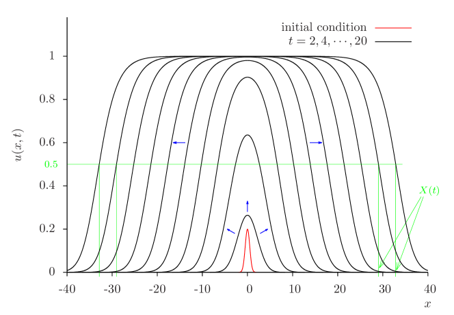
So far, we have solved the diffusion problem in the case of free boundary conditions (The particle could diffuse on the whole lattice, without any restriction). Let us now put an absorptive boundary at position $X<0$. If the particle hits the position $x=X$, it is lost, and the random walk stops. The solution to this problem will be used later to address the branching random walk.

Figure 3: Three realizations of the continuous Brownian with an absorptive boundary at $X=-100$ up to $t=10000$. One of the paths hits the boundary.

Let us state mathematically the problem: We need to solve the diffusion equation $\partial_{t}P=\partial_{x}^{2}P$ for $x>X$, with the initial condition $P(x,0)=\delta(x)$, and the boundary condition $P(X,t)=0$. It is actually possible to replace this boundary problem by an initial-value problem, taking advantage of the linearity of the diffusion equation. It is easy to check that the initial-value problem

$$\partial_{t}P=\partial_{x}^{2}P,\ P(x,0)=\delta(x)-\delta(x-2X)$$ (18)

is equivalent to the boundary problem as long as $x\geq X$. This is the so-called method of images. The solution is then just the difference of Eq. (11) and of the latter translated by $2X$:

$$P(x,t)=\frac{1}{\sqrt{4\pi t}}\left[e^{-\frac{x^{2}}{4t}}-e^{-\frac{(x-2X)^{2}}{4t}}\right].$$ (19)

This function is represented in Fig. 4. Let us take the large-time limit of this expression. We assume that $X$ be of order 1. We may then write

$$\begin{split}P(x,t)&=\frac{1}{\sqrt{4\pi t}}\left[e^{-\frac{[(x-X)+X]^{2}}{4t}}-e^{-\frac{[(x-X)-X]^{2}}{4t}}\right]\\ &=e^{-\frac{(x-X)^{2}}{4t}}\left[e^{-\frac{X(x-X)}{2t}}-e^{\frac{X(x-X)}{2t}}\right]e^{\frac{X^{2}}{4t}}\\ &\underset{t\gg 1}{\simeq}\frac{1}{\sqrt{\pi t}}e^{-\frac{(x-X)^{2}}{4t}}\sinh\frac{(-X)(x-X)}{2t}.\end{split}$$ (20)

The remaining Gaussian factor is significant only in the range $x-X\ll\sqrt{t}\ll t$. The second inequality is trivial for large $t$. When the first inequality is satisfied, one may expand the $\sinh$ factor, and one gets

$$P(x,t)=\frac{(-X)}{2\sqrt{\pi}}\frac{(x-X)}{t^{3/2}}e^{-\frac{(x-X)^{2}}{4t}}.$$ (21)

Figure 4: Probability density $P(x,t)$ to find the particle at position $x$ at time $t$ as a function of $x$ for three different times: $t=200$ (most peaked curve), $t=1000$ and $t=10000$ (flattest curve). We consider two different boundary conditions: free boundary conditions (black curves, Eq. (11)) and absorptive boundary condition at $X=-100$ (red curves, Eq. (19)). The shaded area represents the forbidden region in the case of an absorptive boundary condition.

Exercise 2.

Show that Eq.(21) is actually an exact solution to the diffusion equation. (Do not use the method of images.)

Exercise 3.

Perform the integral

$$\int_{X}^{+\infty}dx\,P(x,t)$$ (22)

and comment on the result. Then, compute the mean value of the position of the particle at time $t$.

1.2 Branching random walk

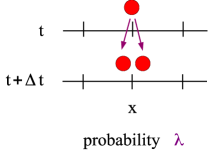
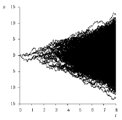
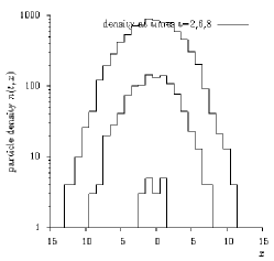
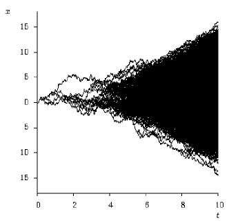
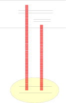
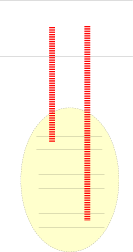
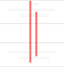
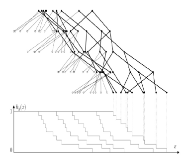
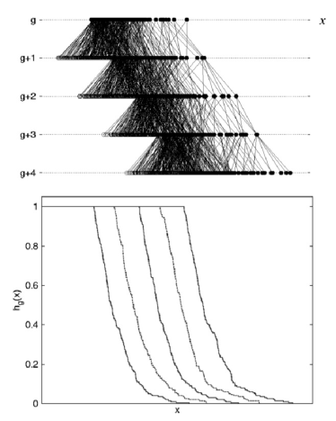
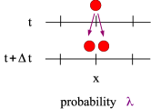
We add a process to the Brownian motion defined in Fig. 1: During the time interval $\Delta t$, each particle may split to two particles on the same site with probability $\lambda$ (see Fig. 5). Numerical simulations of realizations of a branching random walk in the continuum limit are shown in Fig. 6. Now at time $t$, one has a distribution of particles, whose number and set of positions are random variables.

Ordinary Brownian motion		Branching

Figure 5: Elementary processes defining the branching random walk on a lattice.

(a)	(b)	(c)

Figure 6: Three realizations of a branching random walk. Top: particle positions as a function of time. Bottom: Corresponding particle number densities in bins of size 1 (logarithmic scale on the $y$-axis) at three different times: $t=2,6$ and 8. In realization (a) and especially (b), the first splittings happen quite late, leading to a total number of particles at later time which is quite low, while in (c), the first splittings are very fast. It is during the low density phase, at the beginning of the evolution, that diffusion is very effective to shift the particle distributions. It is clear in these figures that the effect of the early-time fluctuations persist to very late times.

Let us establish an equation for the average number of particles on site $x$ at time $t+\Delta t$, given the full distribution of particles at time $t$. On the average, a fraction $1-2\mu$ of the $n(x,t)$ particles already present at $x$ at time $t$ does not move and hence contributes to $\langle n(x,t+\Delta t)\rangle_{[t,t+\Delta t]}$ (the subscript ${[t,t+\Delta t]}$ means that the average is taken in the corresponding time interval only), the fraction $\mu$ of the particles at $x-\Delta x$ add to the latter, as well as the same fraction $\mu$ of the particles on site $x+\Delta x$. Finally, a fraction $\lambda$ of the $n(x,t)$ split, which adds $\lambda n(x,t)$ to $\langle n(x,t+\Delta t)\rangle_{[t,t+\Delta t]}$. This leads to the equation

$$\langle n(x,t+\Delta t)\rangle_{[t,t+\Delta t]}=n(x,t)(1-2\mu)+n(x-\Delta x,t)\mu+n(x+\Delta x,t)\mu+\lambda n(x,t).$$ (23)

Now in order to get a closed equation, we may average over the whole history between time $0$ and time $t$:

$$\langle n(x,t+\Delta t)\rangle-\langle n(x,t)\rangle=\mu\left[\langle n(x+\Delta x,t)\rangle+\langle n(x-\Delta x,t)\rangle-2\langle n(x,t)\rangle\right]+\lambda\langle n(x,t)\rangle.$$ (24)

We can set $\lambda=\Delta t$ and $\mu(\Delta x)^{2}=\Delta t$, and take to limits $\Delta x,\Delta t\rightarrow 0$ to arrive at a partial differential equation:

$${\partial_{t}}\langle n\rangle=\partial_{x}^{2}\langle n\rangle+\langle n\rangle.$$ (25)

The first term in the right-hand side of this equation is a diffusion term, while the second term represents the branchings. Using the integral transform (6) (we call $\tilde{n}(\gamma,t)$ the transform of $\langle n(x,t)\rangle$), we obtain an equation which can be viewed as an ordinary differential equation

$$\frac{d\tilde{n}(\gamma,t)}{dt}=(\gamma^{2}+1)\tilde{n}(\gamma,t),$$ (26)

with the initial condition $\tilde{n}(\gamma,t=0)=1$. The solution is again trivial:

$$\tilde{n}(\gamma,t)=e^{(\gamma^{2}+1)t},$$ (27)

and transforming back to $\langle n\rangle$ using the inverse Mellin transform (6):

$$\langle n(x,t)\rangle=\int\frac{d\gamma}{2i\pi}e^{-\gamma x+(\gamma^{2}+1)t}=\frac{1}{\sqrt{4\pi t}}{\exp\left({t-\frac{x^{2}}{4t}}\right)}.$$ (28)

This is an exact result, and was obtained very simply.

The function (28) is represented in Fig. 7.

Figure 7: Mean particle number $\langle n(x,t)\rangle$ (Eq. (28)) generated by a branching random walk for three different times: $t=3,4,5$. The values of $x$ for which $\langle n(x,t)\rangle=1$ are also represented for $t=3$ and $t=5$.

There are other quantities related to the branching random walk for which an analytical expression is much less easy to get. One of them is the mean position of the rightmost (or leftmost) particle in the branching random walk, as a function of time.

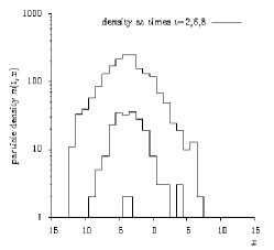
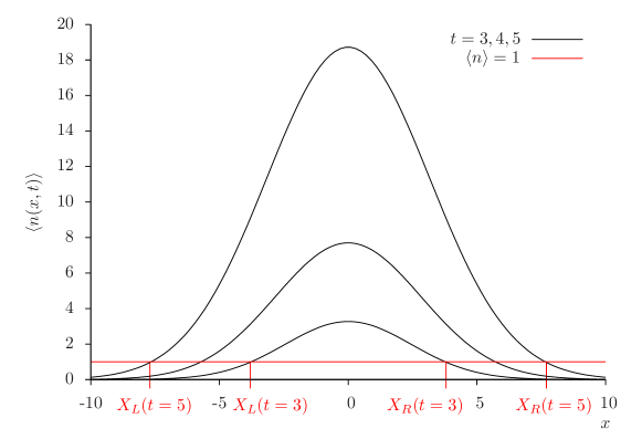
Let us first try the most naive approach. We assume that the mean particle density $\langle n\rangle$ reflects the particle distribution in each realization. Then, the position $X_{R}(t)$, $X_{L}(t)$ of the rightmost and leftmost particles respectively would be the values of $x$ for which $\langle n(x,t)\rangle$ is say 1 (see Fig. 7). To determine $X_{R,L}(t)$, we just need to solve $\langle n(X_{R,L}(t),t)\rangle=1$. From Eq. (28), we find, at large $t$,

$$X_{R}(t)=2t-\frac{1}{2}\ln t+\text{const},\ X_{L}(t)=-2t+\frac{1}{2}\ln t+\text{const}.$$ (29)

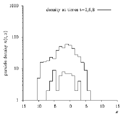
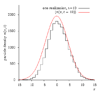
This result is actually not fully correct, which is not so suprising given that there are large fluctuations between realizations in the particle number densities (see Fig. 7, and Fig. 8 for a comparison between one realization and the mean density). It turns out however that the first terms $\pm 2t$ are the correct ones. The fact that the subleading terms are logarithmic is also correct, but the coefficients of these logs are wrong. In order to obtain the correct result, we need to establish an exact equation for the probability distribution $p(X,t)$ of the position ($X$) of say the rightmost particle in the branching random walk.

(a)	(b)

Figure 8: Another realization of a branching random walk until $t=10$. (a) Trajectories of the particles as a function of time. (b) Comparison between the particle density in the realization at time $t=10$ and the mean particle density (red continuous line). We selected a particular realization for which the density is not very different in shape from the latter. There are actually large event-by-event variations with respect to the mean. One important feature of the realization is that there is of course a leftmost and a rightmost occupied bin, while $\langle n(x,t>0)\rangle$ is nonzero for all $x$.

To this aim, let us introduce the probability $Q(x,t)$ that at time $t$, all particles be on the left of position $x$, starting from one single particle at position 0. We establish an evolution equation for $Q(x,t)$ in the same way as for $P$ in the case of the Brownian motion or of $\langle n\rangle$ above, that is by trying to relate $Q$ at time $t+\Delta t$ to $Q$ at time $t$. However, in the present case, it is better to divide the time interval as $[0,t+\Delta t]=[0,\Delta t]\cup[\Delta t,t+\Delta t]$, namely to add the small interval $\Delta t$ at the beginning when the system still consists in a single particle.

After the first time step of size $\Delta t$, the system consists either (i) in a single particle at position $+\Delta x$ (this happens with probability $\mu$), or (ii) in a single particle at position $-\Delta x$ (with the same probability), or (iii) of two particles at position $0$ (with probability $\lambda$), or finally (iv) of one single particle at position 0 if nothing happens in the first time step (probability $1-2\mu-\lambda$). In case (i), the probability $Q(x,t+\Delta t)$ that all particles be on the left of position $x$ at time $t+\Delta t$ is the probability that all particles be on the left of $x$ after evolution of a particle initially at $\Delta x$ over a time interval $t$, namely $Q(x-\Delta x,t)$. In case (ii), the same line of reasoning leads to $Q(x+\Delta x,t)$. In the third case, at time $\Delta t$, we have two particles at position 0, which evolve independently of each other over $t$ additional steps of time. Hence the probability that all particles be to the left of $x$ at time $t+\Delta t$ is the probability that all particles of both independent branching random walks be to the left of $x$, namely $[Q(x,t)]^{2}$. The assumption that the particles have independent evolutions is of course crucial here to obtain this term as a simple product. Case (iv) is trivial.

Translating this discussion into a mathematical expression, we get the equation

$$Q(x,t+\Delta t)=\mu\left[Q(x-\Delta x,t)+Q(x+\Delta x,t)\right]+\lambda Q^{2}(x,t)+(1-2\mu-\lambda)Q(x,t),$$ (30)

which can be recast as a finite-difference evolution equation:

$$Q(x,t+\Delta t)=Q(x,t)+\mu\left[Q(x-\Delta x,t)+Q(x+\Delta x,t)-2Q(x,t)\right]+\lambda\left[Q^{2}(x,t)-Q(x,t)\right].$$ (31)

Taking the usual continuous limit ($\Delta t,\Delta x\rightarrow 0$ with $\mu(\Delta x)^{2}=\Delta t$ and $\lambda=\Delta t$), we arrive at a nonlinear partial differential equation called the Fisher-Kolmogorov-Petrovsky-Piscounov (FKPP) equation

$$\frac{\partial Q}{\partial t}=\frac{\partial^{2}Q}{\partial x^{2}}-Q+Q^{2}.$$ (32)

At $t=0$, if one starts with a single particle at position 0, then obviously the probability $Q(x,0)$ is 1 for $x>0$ and $0$ for $x\leq 0$, namely

$$Q(x,0)=\theta(x).$$ (33)

Recalling the definition of $Q$, we see immediately that the probability distribution $p(x,t)$ of the position of the rightmost particle is just the $x$-derivative of $Q$:

$$p(X,t)=\frac{\partial}{\partial x}Q(x,t)|_{x=X}$$ (34)

and hence the average position of the rightmost particle reads

$$X_{R}(t)=\langle x\rangle_{t}=\int_{-\infty}^{+\infty}dx\,x\,p(x,t)=\int_{-\infty}^{+\infty}dx\,x\,\frac{\partial}{\partial x}Q(x,t).$$ (35)

Exercise 4.

We introduce the number $N(t)$ of particles at time $t$ in a given realization, the set $\{x_{i}(t)\}$ of their positions, and a function $f(x)$. Prove that

$$F(x,t)\equiv\left\langle\prod_{i=1}^{N(t)}f(x-x_{i}(t))\right\rangle$$ (36)

obeys the FKPP equation with $f(x)$ as initial condition.

In these lectures, we shall mainly use an alternative form of the FKPP equation, which is obeyed by the function $u\equiv 1-Q$:

$$\partial_{t}u=\partial_{x}^{2}u+u-u^{2}.$$ (37)

Of course, $u(x,t)$ is simply the probability that at least one particle be located to the right of $x$ at time $t$.

Numerical project.

Branching random walks on a spacetime lattice are relatively easy to implement numerically. It is useful to write a code which generates realizations of such a model, in order to be able to “play” with the model and build up an intuition of its behavior.

Consider the model described at the begining of this section. (We may set, for example, $\mu=\lambda=\Delta t=10^{-2}$ and $\Delta x=1$).

The most straightforward method would be to simulate the behavior of each individual particle as one increases time from $t$ to $t+\Delta t$, namely to “decide” for each particle whether it moves right, left, duplicates, or stays as is in this time interval. However, the complexity of this method is linear in the number of particles, that is to say exponential in time, and thus becomes unpractical after a few times steps.

However, since we have a spacetime lattice and since the particles are indistinguishable, we can instead decide for each site how many particles move right, how many move left and so on.

The first step of our project is to prove that given a number $n$ of particles on a particular site at time $t$, the joint distribution of the number $n_{L}$ of particles that move left, $n_{R}$ that move right, and $n_{+}$ that duplicate is given by the multinomial law

$$P(n_{L},n_{R},n_{+})=\binom{n}{n_{L},n_{R},n_{+},n-n_{L}-n_{R}-n_{+}}\mu^{n_{L}+n_{R}}\lambda^{n_{+}}(1-2\mu-\lambda)^{n-n_{L}-n_{R}-n_{+}},$$ (38)

where the multinomial coefficient is a generalization of the binomial coefficient:

$$\binom{n}{k_{1},k_{2},\cdots,k_{j}}=\frac{n!}{k_{1}!k_{2}!\cdots k_{j}!}\ \ \text{with}\ \ n=\sum_{i=1}^{j}k_{i}.$$ (39)

Since according to our naive estimate, the number of sites which are occupied at time $t$ grows linearly with $t$, the complexity also depends linearly on $t$.

It is now an easy programming exercise to implement this evolution rule. The only practical issue may be with the bookkeeping of the moves of the particles.

   Intermediate recap
We have introduced branching random walks in one space dimension. It is a class of stochastic models with basically two elementary processes which determine the dynamics: diffusion in space, and branching. We have seen that the mean density of particles obeys a simple linear partial differential equation. Other “observables” on this branching random walk such as the mean position of the boundaries (namely of the rightmost/leftmost particles) are derived from nonlinear partial differential equations instead, such as the FKPP equation (37) in the simplest case of branching Brownian motion (continuous space and time) with diffusion constant and branching rate both set to unity. $\blacksquare$   

2 Solving the FKPP equation

This section is dedicated to finding solutions, or rather, properties of the solutions to the FKPP equation

$$\partial_{t}u=\partial_{x}^{2}u+u-u^{2}.$$ (37^′)

Our approach will essentially be heuristic; We will nevertheless state a fundamental mathematical theorem on the convergence of the solutions to traveling waves at large times. Then, we shall generalize the obtained properties to a wider class of equations.

2.1 Heuristic analysis of the equation

Figure 9: Numerical solution of the FKPP equation (37) at different times (black curves), starting from a localized initial condition (red curve which represents Eq. (41) for $\varepsilon=0.3$). The blue arrows indicate the sense of the evolution from one time to the next one.

We first look for spatially homogeneous solutions $u(x,t)=U(t)$. Then Eq. (37) reduces to the simple first-order equation

$$U^{\prime}(t)=U(t)-U^{2}(t),$$ (40)

whose solution is trivial. We shall however limit ourselves to analyze the two fixed points $U=0$ and $U=1$. The latter is stable, while the former is unstable. In order to see these facts, we consider infinitesimal perturbations of these fixed points, and follow their $t$ evolution.

If $U(t=0)=\varepsilon\ll 1$, then $U(t)\simeq\varepsilon e^{t}$ (as long as $t\ll\ln 1/\varepsilon$). A small perturbation grows exponentially with time, which means that $U=0$ is indeed an unstable fixed point. If one perturbs instead the other fixed point by setting the initial condition $U(t=0)=1-\varepsilon$, then $U(t)\simeq 1-\varepsilon e^{-2t}$, and thus $U$ goes back to the fixed point $U=1$, which means that it is stable.

We go back to the full equation (37), and we start the evolution with a localized, small initial condition, say

$$u(x,t=0)=\frac{\varepsilon}{\sqrt{2\pi}}e^{-\frac{x^{2}}{2\varepsilon^{2}}}\ \text{with}\ \varepsilon\ll 1.$$ (41)

This is a perturbation to the unstable fixed point, and thus we know that it should grow exponentially with time. At small times ($t\ll\ln 1/\varepsilon$), $u\ll 1$ and the nonlinear term in Eq. (37) can be neglected compared to the linear growth term. Thus the FKPP equation may be replaced by its linearized part

$$\partial_{t}u=\partial_{x}^{2}u+u,$$ (42)

which encodes an exponential growth in time and a diffusion in space. At large enough $t$, there are regions in $x$ in which $u$ reaches 1, and where the nonlinear term is no longer negligible. Actually, it starts to compensate the linear growth term, and tames the exponential growth, bringing $u$ to its stable fixed point. The growth may continue only at larger values of $|x|$. Thus, wave fronts form, and move to larger values of $|x|$ as time elapses. These fronts are called “traveling waves”, and are characterized by their position $X(t)$ and their shape in the comoving frame. We show a numerical solution of the FKPP equation in Fig. 9 in order to illustrate the dynamics just described, and the formation of the traveling wave starting from a small localized initial condition.

This intuitive discussion is actually backed by a rigorous mathematical theorem, which we are going to state in the following section.

2.2 Bramson’s theorem: traveling waves

We are going to put the theorem in a general form that will be easy to take over to different kinds of branching random walks later. To this aim, we introduce notations that may seem arbitrary at this stage, but whose meaning will become transparent later on.

Let us define the function

$$v(\gamma)=\gamma+\frac{1}{\gamma},$$ (43)

which is determined by the linearized part of the FKPP equation (Eq. (42)), see below. Let us also introduce $\gamma_{0}$, the solution of $v^{\prime}(\gamma_{0})=0$.

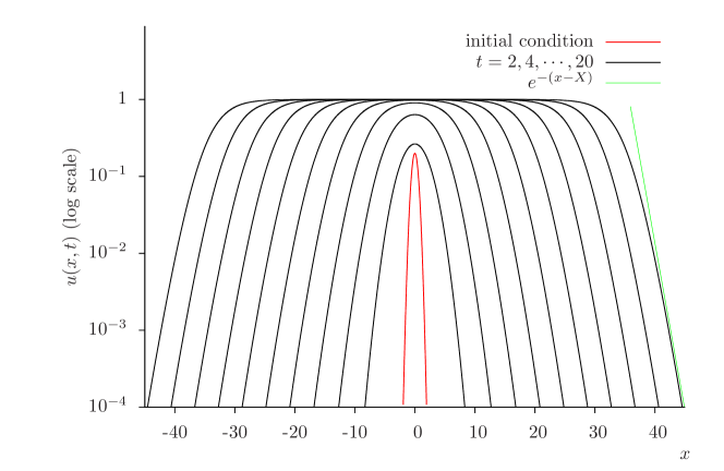
The theorem states that if one chooses an initial condition such that $u(x,0)$ decreases smoothly from 1 to 0 as $x$ goes from $-\infty$ to $+\infty$, with the asymptotic behavior

$$u(x,0)\underset{x\rightarrow+\infty}{\sim}e^{-\beta x}\ \text{with $\beta\neq\gamma_{0}$}\ \ \text{or}\ \ u(x,0)\underset{x\rightarrow+\infty}{\sim}x^{\nu}e^{-\gamma_{0}x},$$ (44)

then, at large time, $u$ becomes a function of a single variable:

$$u(x,t)\underset{t\rightarrow+\infty}{\sim}{\cal U}(x-X^{(\beta)}(t)),$$ (45)

where

$$X^{(\beta)}(t)=\begin{cases}v(\beta)t+{\cal O}(1)&\text{for $\beta<\gamma_{0}$ or ($\beta=\gamma_{0}$ and $\nu<-2$)}\\ v(\gamma_{0})t+\frac{\nu-1}{2\gamma_{0}}\ln t+{\cal O}(1)&\text{for $\beta=\gamma_{0}$ and $\nu>-2$}\\ v(\gamma_{0})t-\frac{3}{2\gamma_{0}}\ln t+{\cal O}(1)&\text{for $\beta>\gamma_{0}$}\end{cases}$$ (46)

Here, $\gamma_{0}=1$ and $v(\gamma_{0})=2$, but we shall deal with variants of the FKPP equation, for which it will be enough to replace the function $v$ and hence the parameters $\gamma_{0}$ and $v(\gamma_{0})$ for the above formulae to apply.

This is (our reformulation of) a theorem which was proved rigorously. In the next sections, we shall motivate these formulae through heuristic arguments.

Note that for applications to QCD, only the last case of Bramson’s theorem will be relevant to us.

2.3 Heuristic derivation of the properties of the traveling waves

2.3.1 Asymptotic shape and velocity

Let us go far to the right of the position $X(t)$ of the wave front. There, the linearized equation

$$\partial_{t}u=\partial_{x}^{2}u+u$$ (42^′)

is a good approximation to the full FKPP equation. We have seen that the solution of such an equation reads (see Eq. (28) with the substitution $\langle n\rangle\rightarrow u$)

$$u(x,t)=\int\frac{d\gamma}{2i\pi}\tilde{u}(\gamma,0)e^{-\gamma x+(\gamma^{2}+1)t}=\int\frac{d\gamma}{2i\pi}\tilde{u}(\gamma,0)e^{-\gamma[x-v(\gamma)t]},$$ (47)

where $v(\gamma)$ is the function given by Eq. (43) and is the velocity of the wave of “wave number” $\gamma$.

We now go to the moving frame defined by the change of coordinates $x=\xi+Vt$, where $V$ is a constant representing the velocity of this new frame with respect to the original one. We choose the initial condition $u(x,t=0)=e^{-\beta x}$ for $x>0$ and $u(x,t=0)=1$ for $x\leq 0$. Then, obviously,

$$\tilde{u}(\gamma,0)=\frac{\beta}{\gamma(\beta-\gamma)}.$$ (48)

In the new frame and with this initial condition,

$$u(\xi,t)=\int\frac{d\gamma}{2i\pi}\left[\frac{\beta}{\gamma(\beta-\gamma)}\right]e^{-\gamma[\xi-(v(\gamma)-V)t]}.$$ (49)

The integration goes over say a straight line parallel to the imaginary axis in the complex $\gamma$ plane, and intersects the real axis between $0$ and $\beta$. If $t$ is a large parameter, we may try and evaluate the integral over $\gamma$ using the saddle-point method. We recall that generically, this method consists in the following approximation:

$$I=\int\frac{d\gamma}{2i\pi}g(\gamma)e^{f(\gamma)t}\underset{\text{$t$ large}}{\sim}\sum_{\gamma_{s}}g(\gamma_{s})e^{f(\gamma_{s})t},$$ (50)

where $\gamma_{s}$ represents the extrema of $f$, namely the solution(s) of the saddle-point equation $f^{\prime}(\gamma_{s})=0$. In our case, the following identifications are in order:

$$I=u(\xi,t),\ g(\gamma)=\frac{\beta}{\gamma(\beta-\gamma)}e^{-\gamma\xi}\ \ \text{and}\ \ f(\gamma)=\gamma[v(\gamma)-V].$$ (51)

The saddle-point equation reads $(\gamma_{s}v(\gamma_{s}))^{\prime}=V$. With $v$ given by Eq. (43), the latter obviously has a single solution. Hence

$$u(\xi,t)=\frac{\beta}{\gamma_{s}(\beta-\gamma_{s})}e^{-\gamma_{s}\xi+\gamma_{s}(v(\gamma_{s})-V)t},$$ (52)

which is an acceptable solution so long as one can move the contour in such a way that it does not hit the singularity at $\gamma=\beta$, so for $\beta>\gamma_{s}$.

Next, one chooses the velocity of the frame $V$ in such a way that the solution be stationary. One easily sees that $V=v(\gamma_{s})$. Together with the saddle-point equation, these equations define $\gamma_{s}$ to be the value $\gamma_{0}$ of $\gamma$ which minimizes $v(\gamma)$, i.e. $v^{\prime}(\gamma_{0})=0$. Hence the actual front velocity at large time is the minimum possible velocity allowed by the dispersion relation, and the shape of the front is $u\sim e^{-\gamma_{0}\xi}$. The convergence towards this shape is seen in Fig. 10.

Figure 10: The same as Fig. 9 but in logarithmic scale in the $y$-axis in order to see the exponential shape $e^{-x}$ setting in at large $t$ and $x$, and progressively replacing the initial Gaussian.

We mention only briefly the case $\beta<\gamma_{s}$, since as we shall see later, is not of interest for QCD. In this case, the dominant contribution to the integral is the pole at $\gamma=\beta$, and thus

$$u(\xi,t)=e^{-\beta\xi+\beta(v(\beta)-V)t}$$ (53)

which can be made stationary by setting $V=v(\beta)$. So in this case, the front velocity at large times is the velocity of the tail of the initial state, whose shape $u\propto e^{-\beta\xi}$ is preserved through the evolution.

From now on, we shall consider a steep enough initial condition, such as $Q(x,t=0)=1-u(x,t=0)=\theta(x)$, or a localized one like Eq. (41).

2.3.2 Finite-time corrections

The full nonlinear problem is of course too difficult to solve. Let us try and replace it by a simpler problem.

From our earlier heuristic analysis, we convinced ourselves that the effect of the nonlinearity is just to tame the exponential growth of $u$ which results from the (linear) branching term in the evolution equation. So it is natural to expect that the wave velocity be determined by the linear part of the latter. The easiest way to represent the effect of the nonlinearity is to replace it with a moving absorptive boundary set at a fixed distance of the position of the front.

We solve the linear equation in the frame moving at velocity 2: $\xi=x-2t$. We define

$$u(x,t)=e^{-\xi}h(\xi,t).$$ (54)

The linear equation (42) on $u$ translates into an equation for $h$. Indeed,

$$\begin{split}\partial_{t}u&=(2h+\dot{\xi}\partial_{\xi}h+\partial_{t}h)e^{-\xi}\\ \partial_{x}u&=(-h+\partial_{\xi}h)e^{-\xi}\\ \partial^{2}_{x}u&=(h-2\partial_{\xi}h+\partial_{\xi}^{2}h)e^{-\xi},\end{split}$$ (55)

with $\dot{\xi}=-2$. Therefore, Eq. (42) reduces to

$$\partial_{t}h=\partial_{\xi}^{2}h,$$ (56)

which is the simple diffusion equation.

We try and put an absorptive boundary in the moving frame at $\xi=0$. Then according to the discussion which led to Eq. (21), the solution of the diffusion equation reads

$$h(\xi,t)\propto\frac{\xi}{t^{3/2}}e^{-\frac{\xi^{2}}{4t}},$$ (57)

namely

$$u(x,t)\propto\xi e^{-\xi-\frac{3}{2}\ln t}e^{-\frac{\xi^{2}}{4t}}.$$ (58)

The lines of constant $u$ correspond to the trajectory of the front. Thus we define the position $\xi_{t}$ of the front in the moving frame as $u(x=2t+\xi_{t},t)=\text{const}$. From Eq. (58), it is clear that at large $t$, $\xi_{t}=-\frac{3}{2}\ln t+\cdots$ hence the position of the front in the original frame reads

$$X(t)=2t+\xi_{t}=2t-\frac{3}{2}\ln t+\cdots$$ (59)

which is Bramson’s result.

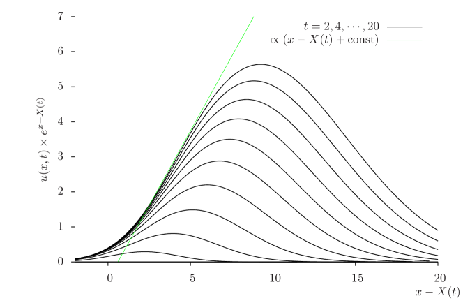
Now, we should adjust the position of the boundary in such a way that it matches a line of constant $u$. We would then get for the shape of $u$:

$$u(x,t)\propto(x-X(t)+\text{const})e^{-(x-X(t))}e^{-\frac{(x-X(t))^{2}}{4t}}.$$ (60)

The shape is best seen if one plots $u(x,t)\times e^{x-X(t)}$ against $x$, which is sometimes called the “reduced front” (see Fig. 11). This function converges to the “scaling” function $\text{const}\times(x-X(t)+\text{const})$ at large times.

Figure 11: Numerical evaluation (as in Fig. 9) of $u(x,t)\times e^{(x-X(t))}$. One sees the convergence to a straight line $\text{const}\times(x-X(t)+\text{const})$ (green line).

The initial problem was to find the probability distribution $p(X,t)$ of the position $X$ of the rightmost particle. It was related to the function $Q$ satisfying the FKPP equation, and thus to $u$ through

$$p(X,t)=\frac{\partial Q(x,t)}{\partial x}|_{x=X}=-\frac{\partial u(x,t)}{\partial x}|_{x=X}.$$ (61)

We leave as an exercise to find the relation between $X(t)$ computed above and the average value of the rightmost particle in the branching random walk:

Exercise 5.

Prove that $\langle X\rangle_{t}$ is related to an integral of $u$:

$$U=\int^{+\infty}dx\,u(x,t)+\text{const}.$$ (62)

How should the lower bound of this integral be set? How should the additive constant be chosen? Relate $U$ to the expectation value of the random variable $X$. Finally, show that, given the fact that $u$ is a traveling wave, $U$ is a way to define the position of the front, namely that at large time, $U=X(t)$.

Recall that the naive estimate of the average position of the rightmost particle gave

$$X_{R}(t)=2t-\frac{1}{2}\ln t+\text{const}$$ (29^′)

(see also Fig. (7)). Comparing to Eq. (59), we see that the leading term ($2t$) was correct, the form of the subleading term ($\propto\ln t$) also, but the coefficient was not the correct one. The nonlinearity/absorptive boundary just changed this coefficient $\frac{1}{2}$ to a $\frac{3}{2}$.

2.4 “Dual” interpretation of the solution to the FKPP equation

The main manifestation of the discreteness of the number of particles is obviously to bring the particle density $n$ in each event to 0 to the right of the rightmost occupied site. This fact is of course neglected in the “mean-field” approximation to branching diffusion in which one replaces $n$ by its expectation value $\langle n\rangle$.

One may try to model discreteness by an absorptive boundary on the linear equation which gives the evolution of the mean number of particles $\langle n\rangle$. In this case, we would solve again a diffusion equation with an absorptive boundary condition. The result would be very similar to the one obtained in the case of the FKPP equation, where the absorptive boundary represented the nonlinearity which forced $u$ to keep less than 1. We would get the following expression, near the right discreteness boundary:

$$\langle n(x,t)\rangle\propto\left(X(t)-x\right)e^{-(x-X(t))-\frac{(x-X(t))^{2}}{4t}}\theta(X(t)-x).$$ (63)

Before, we had a deterministic nonlinear equation (37), which we replaced by its linearized approximation (42) supplemented with an absorptive boundary. In the present case, the time evolution of the branching random walk is a priori represented by a stochastic equation. We replace the latter by its mean-field approximation also supplemented with an absorptive boundary with mimics the main origin of the noise, namely the discreteness of the number of particles. The two problems are very similar from the mathematical point of view, so it is not surprising that the position of the “discreteness boundary”, namely of the rightmost particle in the branching random walk, has the time dependence of the position of the FKPP traveling wave (59).

Actually, there would be a difference between the two calculations if we went to the next order in the large-$t$ expansion, a fact which we shall comment at the end of this chapter.

2.5 Generalization to other branching-diffusion processes

We are going to extend the results just obtained in the case of the simple branching random walk to more general branching-diffusion processes. In particular, we will consider models in discrete space and/or time, which are more suitable for numerical implementation.

This generalization mainly relies on the observation that what we have done only depends on the linear branching-diffusion kernel.

We had the equation

$$\partial_{t}u=\partial_{x}^{2}u+u.$$ (42^′)

The eigenfunctions of the kernel were $e^{-\gamma x}$, and the corresponding eigenvalues $\chi(\gamma)=\gamma^{2}+1$. More precisely, $u(x,t)=e^{-\gamma(x-vt)}$ solves Eq. (42) provided that $v$ be related to the eigenvalues through $v(\gamma)=\chi(\gamma)/\gamma$. We saw that at large times, the eigenfunction $e^{-\gamma_{0}x}$ dominates when one looks in the vicinity of a given value of $u$, where $\gamma_{0}$ solves $v^{\prime}(\gamma_{0})=0$.

All this was very general: One may replace $\chi(\gamma)$ by the eigenvalues of any branching-diffusion kernel. Let us go back to the solution to the linearized equation expressed in a more general form, namely with the help of $\chi(\gamma)$:

$$u(x,t)=\int\frac{d\gamma}{2i\pi}\tilde{u}(\gamma,0)e^{-\gamma x+\chi(\gamma)t}.$$ (64)

Since we know that large times single out the wave number $\gamma_{0}$, we expand $\chi(\gamma)$ to second order around some $\gamma_{0}$, take the prefactor $\tilde{u}(\gamma,0)$ at $\gamma_{0}$, and eventually go to the frame moving at velocity $v(\gamma_{0})$ by redefining $x$ as $x=\xi+v(\gamma_{0})t$:

$$\begin{split}u(x,t)&\simeq\tilde{u}(\gamma_{0},0)\int\frac{d\gamma}{2i\pi}e^{-\gamma x+[\chi(\gamma_{0})+(\gamma-\gamma_{0})\chi^{\prime}(\gamma_{0})+\frac{1}{2}(\gamma-\gamma_{0})^{2}\chi^{\prime\prime}(\gamma_{0})]t}\\ &=\tilde{u}(\gamma_{0},0)\int\frac{d\gamma}{2i\pi}e^{-\gamma\xi+\left[\chi(\gamma_{0})-\gamma v(\gamma_{0})+(\gamma-\gamma_{0})\chi^{\prime}(\gamma_{0})+\frac{1}{2}(\gamma-\gamma_{0})^{2}\chi^{\prime\prime}(\gamma_{0})\right]t}\\ &=\tilde{u}(\gamma_{0},0)e^{-\gamma_{0}\xi}\int_{c-i\infty}^{c+i\infty}\frac{d\gamma}{2i\pi}e^{-(\gamma-\gamma_{0})\xi+\frac{1}{2}(\gamma-\gamma_{0})^{2}\chi^{\prime\prime}(\gamma_{0})t}\\ &=\tilde{u}(\gamma_{0},0)e^{-\gamma_{0}\xi}\int_{c+\gamma_{0}-i\infty}^{c+\gamma_{0}+i\infty}\frac{d\gamma}{2i\pi}e^{-\gamma\xi+\frac{1}{2}\gamma^{2}\chi^{\prime\prime}(\gamma_{0})t}\\ &=\tilde{u}(\gamma_{0},0)e^{-\gamma_{0}\xi-\frac{\xi^{2}}{2\chi^{\prime\prime}(\gamma_{0})t}}\int_{\left(c+\gamma_{0}+\frac{\xi}{\chi^{\prime\prime}(\gamma_{0})t}\right)-i\infty}^{\left(c+\gamma_{0}+\frac{\xi}{\chi^{\prime\prime}(\gamma_{0})t}\right)+i\infty}\frac{d\gamma}{2i\pi}e^{\frac{1}{2}\chi^{\prime\prime}(\gamma_{0})t\gamma^{2}}.\end{split}$$ (65)

The next step is to shift the integration contour to make it coincide with the imaginary axis, and then to write $\gamma=i\nu$. The remaining integral is then just an ordinary Gaussian integral:

$$\int_{-\infty}^{+\infty}\frac{d\nu}{2\pi}e^{-\frac{1}{2}\chi^{\prime\prime}(\gamma_{0})t\nu^{2}}=\frac{1}{\sqrt{2\pi\chi^{\prime\prime}(\gamma_{0})t}}.$$ (66)

The prefactor in $u$ stemming from this integral is proportional to $1/\sqrt{t}$ for free boundary conditions. If we had a fixed absorptive boundary condition instead, we would just need to replace it by $\xi/t^{3/2}$.

We see that the procedure to find the shape and position of the front is the same as in the case of the simple FKPP equation. Only a few constants differ. The solution eventually reads

$$u(x,t)\propto(x-X(t))e^{-\gamma_{0}(x-X(t))}e^{-\frac{(x-X(t))^{2}}{2\chi^{\prime\prime}(\gamma_{0})t}},\ \ \text{where}\ \ X(t)=\chi^{\prime}(\gamma_{0})t-\frac{3}{2\gamma_{0}}\ln t+\text{const}.$$ (67)

This formula applies to a variety of stochastic processes. It is enough to compute the relevant eigenvalue $\chi(\gamma)$. Let us give a few examples:

• Branching diffusion in continuous space and time with diffusion constant $D=1$. The equation which gives the time evolution of the probability distribution of the position of the rightmost particle is the FKPP equation

  $$\partial_{t}u=\partial_{x}^{2}u+u-u^{2},$$ (37^′)

  and we have seen that $\chi(\gamma)=\gamma^{2}+1$, hence $v(\gamma)=\gamma+1/\gamma$. From the saddle-point equation, $\gamma_{0}=1$, $v(\gamma_{0})=2$, $\chi^{\prime\prime}(\gamma_{0})=2$. Replacing these constants in Eq. (67), we check that we get back the results obtained earlier (compare to Eq. (59) and (60)).

• Branching random walk on a lattice in space and time. The equivalent of the FKPP equation for this process is the following finite-difference equation:

  $$u(x,t+\Delta t)=u(x,t)+\mu\left[u(x+\Delta x,t)+u(x-\Delta x,t)-2u(x,t)\right]\\ +\lambda u(x,t)\left[1-u(x,t)\right].$$ (68)

  Looking for solutions of the linearized equation in the form $u(x,t)=e^{-\gamma(x-v(\gamma)t)}$, we find

  $$v(\gamma)=\frac{\chi(\gamma)}{\gamma}=\frac{1}{\gamma\Delta t}\ln\left[1+\lambda+\mu\left(e^{-\gamma\Delta x}+e^{\gamma\Delta x}-2\right)\right].$$ (69)

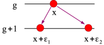
• Population evolution model (biological context). Consider a population (i.e. a set of individuals). Each individual is characterized by a unique real number $x$ called the “fitness”. We define the time evolution by the following rule: Each individual with fitness $x$ present in the population at “generation” number $t$ is replaced at $t+1$ by two offspring, which have respective fitnesses $x_{1}$ and $x_{2}$ such that

  $$x_{1}=x+\varepsilon_{1},\ x_{2}=x+\varepsilon_{2},$$ (70)

  where $\varepsilon_{1},\varepsilon_{2}$ are random numbers distributed according to a “local enough” probability distribution $\rho(\varepsilon)$ (for example $\rho(\varepsilon)=e^{-|\varepsilon|}/2$). Thus the population doubles at each generation, and the individuals diffuse in fitness.

  Exercise 6.

  Write the expression of $v(\gamma)$ in this case, as a functional of $\rho$.
  Hint: Start with a population made of a single individual at $t=0$, at position $x=0$.

• Last but not least, the evolution of scattering amplitudes with the rapidity (i.e. the logarithm of the center-of-mass energy squared) is given by an equation established in QCD which has a lot in common with the FKPP equation. This is basically due to the fact that gluons may branch. We are going to specialize to QCD in Sec. 3.

   Intermediate recap
We have analyzed the FKPP equation (37) and understood some properties of the solutions. Essentially, at least for large times, the FKPP equation admits traveling wave solutions, namely fronts which just translate in $x$ at a constant velocity. Starting with appropriate initial conditions, the traveling wave is reached asymptotically, and its velocity depends on the “steepness” of the initial condition. Bramson’s theorem provides the expression for the velocity and its finite-time corrections. We rederived it (Eq. (59)) in a heuristic approach consisting in replacing the nonlinearity by a moving absorptive boundary, and we got also the shape of the front (60). We then explained how equivalent results may be obtained for a more general branching random walk characterized by the kernel eigenvalues $\chi(\gamma)$:

$$u(x,t)\propto(x-X(t))e^{-\gamma_{0}(x-X(t))}e^{-\frac{(x-X(t))^{2}}{2\chi^{\prime\prime}(\gamma_{0})t}},\ \ \text{where}\ \ X(t)=\chi^{\prime}(\gamma_{0})t-\frac{3}{2\gamma_{0}}\ln t+\text{const},$$ (67)

where $\gamma_{0}$ solves $\chi^{\prime}(\gamma_{0})=\chi(\gamma_{0})/\gamma_{0}$. This is the main result of this section, and holds for a steep enough initial condition. $\blacksquare$   

To go further
The derivation of the velocity of the traveling wave and the shape of the front can be done a bit more rigorously, but in the same spirit of these lectures: see Ref. [vS03]. It is also possible to compute the next term in the expansion of the position of the FKPP front $X(t)$ given in Eqs. (59),(67) by refining the “moving boundary method”. One finds

$$X(t)=\chi^{\prime}(\gamma_{0})t-\frac{3}{2\gamma_{0}}\ln t+\text{const}-\frac{3}{\gamma_{0}^{2}}\sqrt{\frac{2\pi}{\chi^{\prime\prime}(\gamma_{0})}}\frac{1}{\sqrt{t}}+\cdots$$ (71)

Since front shape and velocity are related, a corresponding correction to the shape of the front is found, see Ref. [EvS00]. We refer the reader interested in the FKPP equation, its solutions and its applications to the extensive review given in Ref. [vS03].

The position of a moving absorptive boundary put in the tail in such a way as to mimic discreteness (as was explained in Sec. 2.4) exhibits a similar correction, but with the opposite sign [MM14b]:

$$X_{R,\text{cutoff}}(t)=\chi^{\prime}(\gamma_{0})t-\frac{3}{2\gamma_{0}}\ln t+\text{const}+\frac{3}{\gamma_{0}^{2}}\sqrt{\frac{2\pi}{\chi^{\prime\prime}(\gamma_{0})}}\frac{1}{\sqrt{t}}+\cdots$$ (72)

The average position of the rightmost particle should be equal to $X(t)$ since the FKPP equation describes the time evolution of its probability distribution. The mismatch between $X(t)$ and $X_{R,\text{cutoff}}(t)$ turns out to be exactly due to the tip fluctuations neglected in the moving boundary mean-field model!

3 Applications to QCD

After our general analysis of branching random walks and of the properties of the solutions to the FKPP equation and its avatars, we are now ready to address the peculiar case of QCD. We shall first briefly recall the formulation of deep-inelastic scattering in QCD at high energy, then explain how branching random walks appear, and eventually take over our knowledge of general branching random walks to QCD scattering amplitudes in order to arrive at predictions and models which may be compared to experimental measurements.

3.1 QCD evolution at very high energies

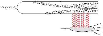
We shall consider deep-inelastic scattering of an electron off some target proton or nucleus in the dipole frame, namely the restframe of the target (see Fig. 12).

Figure 12: Example of graph contributing to deep-inelastic scattering of an electron/positron off a proton/nucleus target at high energy without quantum evolution. The electron emits a virtual photon which interacts with the target through a quark-antiquark fluctuation. $x_{0}$ and $x_{1}$ are the coordinates of the quark and of the antiquark respectively in the (two-dimensional) transverse plane, $z$ is the fraction of the momentum of the photon carried by the quark.

On the target side, we know from general principles that the most probable states of the proton/nucleus at very high energies are dense states of gluons. On the electron side, the electron can be seen as a Weizsäker-Williams cloud of virtual photons of virtuality say $Q^{2}=-q^{2}$, where $q$ is the four-momentum of the photon. Since the latter cannot interact directly with gluons, it splits into a quark-antiquark pair. This pair, being globally color neutral, is a color dipole. At lowest order in the coupling constants, the photon-target cross section reads

$$\sigma^{\gamma^{*}p/A}(Q^{2},y)=\int d^{2}{x_{01}}dz|\psi^{Q}(x_{01},z)|^{2}\int d^{2}b\,2\,\text{Re}(1-S(x_{01},b,y))$$ (73)

where $S(x_{01},b,y)$ is the $S$-matrix element for the elastic scattering of a dipole of size $x_{01}\equiv x_{0}-x_{1}$ (a two-dimensional vector) at rapidity $y$ and impact parameter $b$ off the target proton/nucleus. The total cross section is obtained from the optical theorem, which explains the presence of the “real part” operator. In our further discussion, we will drop the impact-parameter dependence almost throughout.

Now in quantum field theory, the states which actually interact are fluctuations of the initial objects (dipole or proton in their fundamental states; see Fig. 13). So we need to compute the probability distribution of the different states (resulting from further fluctuations) at the time of the interaction.

Figure 13: Example of graph contributing to the quantum evolution of the deep-inelastic scattering process at very high energy.

At high energies, as already mentioned, the dominant fluctuations are dense states of soft gluons. To compute their probabilities at leading order when the coupling constant is small and the rapidity large, it is enough to consider the successive emissions of softer and softer gluons: Eventually, it is the process $\text{gluon}\rightarrow\text{gluon}+\text{gluon}$ which gives the main contribution. Already at this stage, we see that this is a branching process, whose realizations are “trees” of gluons. There is also diffusion since the gluons which result from the branching do not have the same (transverse) momentum as the parent gluon. We need to perform a calculation in the framework of QCD to make this statement precise and useful in practice.

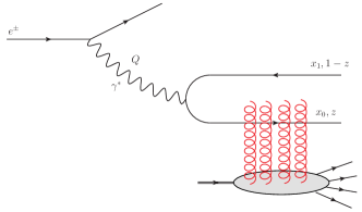
We start with one quark-antiquark color neutral pair (i.e. one color dipole), at rapidity 0: In DIS, this is the $q\bar{q}$ component of the photon wave function. The lowest-order fluctuation is a $q\bar{q}+\text{gluon}$ state. We shall compute first the probability to observe such a state at the time of the interaction starting at lightcone time $\tau=-\infty$ with a bare $q\bar{q}$ pair. Let us denote the quark momentum by $k_{1}$, and the antiquark momentum by $p-k_{1}$. The two graphs contributing to the probability amplitude are represented in Fig. 14. The emitted gluon possesses the momentum $k_{2}$.

It turns out that switching from transverse momentum to transverse coordinates simplifies a lot the problem. Physically, this stems from the fact that high energies, the coordinates of a fast particle are not altered by the interaction nor by the radiation of a soft gluon. Hence we shall go to two-dimensional Fourier space, and introduce the coordinates $x_{0}$ for the quark, $x_{1}$ for the antiquark, $x_{2}$ for the gluon.

$+$

Figure 14: Lightcone perturbation theory graphs contributing to the amplitude for the emission of a gluon by a quark-antiquark pair.

After taking the modulus squared of the graphs shown in Fig. 14 and summing over the polarization and the color of the emitted gluon, the result reads [Mue94]

$$dP(x_{01}\rightarrow x_{02},x_{12})=\frac{2\alpha_{s}C_{F}}{\pi}dy\frac{d^{2}x_{2}}{2\pi}\frac{x_{01}^{2}}{x_{02}^{2}x_{12}^{2}},$$ (74)

where $y$ is the rapidity of the gluon, $y=\ln k_{2+}$ and thus $dy=dk_{2+}/{k_{2+}}$.

Let us comment on this formula. First, the emission probability is of course proportional to the strong coupling constant $\alpha_{s}$, and to the $SU(N_{c})$ Casimir of the fundamental representation $C_{F}$ since we have summed over the colors of the emitted gluon. The differential element comes from the phase space of the gluon. The probability exhibits the two types of singularities present in gauge theories: the soft singularity, which gives a logarithmic divergence to the probability integrated over the “+” component of the gluon momentum $k_{2+}$, and the collinear singularity in the last factor, which enhances the weight of the configurations in which the gluon is emitted collinearly either to the quark or to the antiquark.

It is convenient to go to the large-number-of-color limit (see Fig. 15), since this limit suppresses the planar diagrams and enables one to interpret gluons as zero-size quark-antiquark pairs. (Moreover, in this limit, $C_{F}\rightarrow N_{c}/2$).

$+$

$+$

$+$

$\equiv$

Figure 15: Graphs contributing to the modulus squared of the amplitude for the emission of a gluon by a quark-antiquark pair in the large-$N_{c}$ limit. The rightmost graph is a convenient representation for the sum of all possible graphs which result in the dipole splitting probability (74).

Under these simplifying (but systematic) assumptions, one obtains the color-dipole model [Mue94].

Indeed, the large-$N_{c}$ limit enables one to interpret the emission of the gluon as the splitting of the initial dipole into two new dipoles. So $dP/dy$ can be interpreted as the rate at which a dipole of size $x_{01}$ splits to two dipoles of respective sizes $x_{02}$, $x_{12}$ when the rapidity is increased by the small quantity $dy$.

One may then iterate this process (see Fig. 16): Thanks again to the large-$N_{c}$ limit in which nonplanar graphs are subdominant, the two dipoles, once emitted, evolve independently of each other. Upon rapidity evolution, we get a cascade of dipoles through dipole branching.

	$\underset{\text{large $N_{c}$}}{\simeq}$			$\underset{\text{large $N_{c}$}}{\simeq}$
(a)			(b)

Figure 16: Example of a planar graph which contributes (a) and a nonplanar graph which does not contribute (b) to the modulus squared of the amplitude for the emission of a gluon by a quark-antiquark pair in the large-$N_{c}$ limit.

We are now going to establish the Balitsky-Kovchegov (BK) equation in the same way as we established the FKPP equation.

3.2 QCD evolution as a branching random walk

Let us compute the $S$-matrix element $S(x_{01},y)$ for the elastic scattering of a dipole of size $x_{01}$ after an evolution over $y$ units of rapidity.

$S(x_{01},y)$ is the probability amplitude (in the sense that $S^{2}$ is the actual probability) that there be no interaction between the initial dipole of size $x_{01}$ and the target, after an evolution over $y$ units of rapidity. At the time of the interaction, the projectile dipole has been replaced by a random collection of $N(y)$ dipoles of sizes $\{r_{i}(y)\}$. Since these dipoles are assumed independent, the probability amplitude that in a particular configuration none of them interact is the product of the $S$-matrix elements (at zero rapidity) of each of them. The average over the different dipole configurations has eventually to be taken. Hence we write

$$S(x_{01},y)=\left\langle\prod_{i=1}^{N(y)}S(r_{i}(y),y=0)\right\rangle.$$ (75)

$S(r,y=0)$, which we may also denote by $S_{\text{el}}(r)$, represents the elementary interaction of a dipole of size $r$ with the target, without any quantum evolution.

Now it is useful to recall that we proved that

$$F(x,t)\equiv\left\langle\prod_{i=1}^{N(t)}f(x-x_{i}(t))\right\rangle$$ (36^′)

obeys the FKPP equation for any function $f$ when $\{x_{i}(t)\}$ is the set of the positions of the $N(t)$ particles generated after a branching random walk starting with a single particle at $x=0$ and running over $t$ units of time. The similarity between the last two equations, Eq. (36) and (75) is obvious: It is enough to identify the functions $S$ to $F$, $S_{\text{el}}$ to $f$, the variables $y$ to $t$, and as we will discover later on, $\ln x_{01}^{2}/r_{i}^{2}$ to $x_{i}$.

However, dipole splitting is not exactly the simple branching random walk which is at the origin of the FKPP equation. It is a more sophisticated stochastic process, and therefore, we shall establish the equivalent of the FKPP equation from scratch.

In order to establish such evolution laws, we try and express $S$ at rapidity $y+dy$ as a function of $S$ at rapidity $y$. To do this, we consider what happens in the small rapidity interval $[0,dy]$: Either the dipole does not split, in which case, for this particular event, the $S$-matrix element would be given by $S_{\text{event}}(x_{01},y+dy)=S(x_{01},y)$, or it splits into two dipoles of respective sizes $x_{02}$ and $x_{12}$, in which case $S_{\text{event}}(x_{01},y+dy)=S(x_{02},y)\times S(x_{12},y)$. The fundamental assumption here is the complete independence of the evolution of the dipoles, leading to the latter factorization. $S(x_{01},y+dy)$ is obtained by averaging $S_{\text{event}}(x_{01},y+dy)$ over these two possible cases. We arrive at a sum of $S$ at rapidity $y$ weighted by the dipole splitting probability in Eq. (74):

$$S(x_{01},y+dy)=\left\langle S_{\text{event}}(x_{01},y+dy)\right\rangle=S(x_{01},y)\left[1-dy\int\frac{dP}{dy}(x_{01}\rightarrow x_{02},x_{12})\right]\\ +dy\int\frac{dP}{dy}(x_{01}\rightarrow x_{02},x_{12})S(x_{02},y)S(x_{12},y).$$ (76)

Letting $dy\rightarrow 0$, we obtain the following integro-differential equation:

$$\partial_{y}S(x_{01},y)=\bar{\alpha}\int\frac{d^{2}x_{2}}{2\pi}\frac{x_{01}^{2}}{x_{02}^{2}x_{12}^{2}}\left[S(x_{02},y)S(x_{12},y)-S(x_{01},y)\right].$$ (77)

This is the Balitsky-Kovchegov (BK) equation. Introducing the scattering amplitude $T=1-S$, we get

$$\partial_{y}T(x_{01},y)=\bar{\alpha}\int\frac{d^{2}x_{2}}{2\pi}\frac{x_{01}^{2}}{x_{02}^{2}x_{12}^{2}}\left[T(x_{02},y)+T(x_{12},y)-T(x_{01},y)-T(x_{02},y)T(x_{12},y)\right].$$ (78)

Let us comment on this equation. It is clear that the nonlinear term, of the form $-TT$, is important only when $T\sim 1$, i.e. when typically more than one dipole interacts with the target (since in this case the probability that there be no interaction $S^{2}=(1-T)^{2}$ tends to 0). The BK equation boils then down to

$$\partial_{y}T(x_{01},y)=\bar{\alpha}\int\frac{d^{2}x_{2}}{2\pi}\frac{x_{01}^{2}}{x_{02}^{2}x_{12}^{2}}\left[T(x_{02},y)+T(x_{12},y)-T(x_{01},y)\right],$$ (79)

which is nothing but the Balitsky-Fadin-Kuraev-Lipatov (BFKL) equation written in coordinate space.

In the following, we shall claim that the BK equation (78) is in the universality class of the FKPP equation (37). To make this more precise, we shall first put the BK equation (or rather, an appropriate approximation of it) in a form in which it is manifestly equivalent to the FKPP equation.

3.3 Mapping the Balitsky-Kovchegov equation to the FKPP equation

Let us first analyze the linear limit of the BK equation for $S\rightarrow 1$, which is the BFKL equation. To this aim, we need to find the eigenfunctions and the corresponding eigenvalues of the BFKL equation.

3.3.1 Calculation of the eigenvalues of the BFKL kernel

We will need a few formulae of complex analysis. First, the Euler gamma function is defined as

$$\Gamma(x)=\int_{0}^{+\infty}dt\,e^{-t}t^{x-1},$$ (80)

whose main property is $x\Gamma(x)=\Gamma(1+x)$. We will also need the Taylor expansion around $\varepsilon=0$ of the ratio

$$\frac{\Gamma(a+n\varepsilon)}{\Gamma(a+m\varepsilon)}=1+(n-m)\varepsilon\psi(a)+o\left(\varepsilon^{2}\right),$$ (81)

where $\psi(x)\equiv\Gamma^{\prime}(x)/\Gamma(x)$ and $n$ and $m$ are two finite numbers. The Euler Beta function is a combination of $\Gamma$ functions and is the result of the following integration (see Appendix A):

$$\int_{0}^{1}dx\,x^{\alpha-1}(1-x)^{\beta-1}=\frac{\Gamma(\alpha)\Gamma(\beta)}{\Gamma(\alpha+\beta)}\equiv B(\alpha,\beta).$$ (82)

The main steps of our calculation will rely on a similar-looking formula, but where the integration extends over the whole complex plane:

$$\int\frac{dzd\bar{z}}{2i\pi}|z|^{2\alpha-2}|1-z|^{2\beta-2}=\frac{\Gamma(\alpha)\Gamma(\beta)}{\Gamma(\alpha+\beta)}\frac{\Gamma(1-\alpha-\beta)}{\Gamma(1-\alpha)\Gamma(1-\beta)}.$$ (83)

This formula is classical in the context of 2-dimensional conformal field theory. For completeness, we propose a derivation in Appendix A.

The action of the BFKL kernel on a function $T$ of the 2-dimensional vector $x_{01}$ reads

$$K\otimes T(x_{01})=\bar{\alpha}\int\frac{d^{2}x_{2}}{2\pi}\frac{x_{01}^{2}}{x_{02}^{2}x_{12}^{2}}\left[T(x_{02})+T(x_{21})-T(x_{01})\right].$$ (84)

Note that the first two terms give identical contributions. We restric ourselves to azimuthally symmetric solutions. It is then natural to look for eigenfunctions of the form

$$T(x)=|x|^{2\gamma}.$$ (85)

(A general solution will be a linear combination of these power functions). We insert Eq. (85) into Eq. (84), and go to complex variables by defining

$$z\equiv\frac{x_{02}^{(1)}+ix_{02}^{(2)}}{x_{01}^{(1)}+ix_{01}^{(2)}}$$ (86)

where the superscripts $(1)$ and $(2)$ label the components of the vector. Then

$$|z|^{2}=\frac{x_{02}^{2}}{x_{01}^{2}},\ \ |1-z|^{2}=\frac{x_{21}^{2}}{x_{01}^{2}},\ \ d^{2}x_{2}=\frac{dzd\bar{z}}{2i}|x_{01}|^{2},$$ (87)

and the action of the kernel on the test functions (85) reads

$$K\otimes T(x_{01})=T(x_{01})\times\bar{\alpha}\chi(\gamma),$$ (88)

where $\chi(\gamma)$ is defined by the following integral:

$$\chi(\gamma)\equiv\int\frac{dzd\bar{z}}{4i\pi}\frac{1}{|z|^{2}|1-z|^{2}}\left(|z|^{2\gamma}+|1-z|^{2\gamma}-1\right).$$ (89)

One easily sees that the power functions are indead eigenfunctions, with eigenvalues $\bar{\alpha}\chi(\gamma)$.

Let us discuss the convergence of the integral defining $\chi(\gamma)$. All terms converge at $z=+\infty$ when $0<\text{Re}(\gamma)<1$. The first term converges also at $z=0$ but diverges at $z=1$. As for the second term, it converges $z=1$ but diverges at $z=0$. The last term diverges both at $z=0$ and $z=1$. Hence one needs to regularize these integrals: We choose to slightly modify the powers of the factors in the kernel:

$$\chi(\gamma)=\lim_{\varepsilon\rightarrow 0}\int\frac{dzd\bar{z}}{4i\pi}\frac{1}{|z|^{2-2\varepsilon}|1-z|^{2-2\varepsilon}}\left(|z|^{2\gamma}+|1-z|^{2\gamma}-1\right)\equiv I_{\gamma}-\frac{1}{2}I_{0},$$ (90)

where

$$I_{\gamma}\equiv\int\frac{dzd\bar{z}}{2i\pi}|z|^{2(\varepsilon+\gamma)-2}|1-z|^{2\varepsilon-2}.$$ (91)

It is straightforward to apply Eq. (83) to $I_{\gamma}$, with $\alpha=\varepsilon+\gamma$ and $\beta=\varepsilon$,

$$\begin{split}I_{\gamma}&=\frac{\Gamma(\varepsilon+\gamma)\Gamma(\varepsilon)}{\Gamma(2\varepsilon+\gamma)}\frac{\Gamma(1-2\varepsilon-\gamma)}{\Gamma(1-\varepsilon-\gamma)\Gamma(1-\varepsilon)}\\ &=\frac{1}{\varepsilon}\frac{\Gamma(1+\varepsilon)}{\Gamma(1-\varepsilon)}\frac{\Gamma(\gamma+\varepsilon)}{\Gamma(\gamma+2\varepsilon)}\frac{\Gamma(1-\gamma-2\varepsilon)}{\Gamma(1-\gamma-\varepsilon)}\\ &=\frac{1}{\varepsilon}\left[1+\varepsilon\left(2\psi(1)-\psi(\gamma)-\psi(1-\gamma)\right)\right]+{\cal O}(\varepsilon).\end{split}$$ (92)

(Going from the first line to the second one makes use of the elementary identity $\Gamma(1+x)=x\Gamma(x)$, while the expansion for small $\varepsilon$ is obtained from Eq. (81)). As expected, Eq. (92) diverges when $\varepsilon\rightarrow 0$. The calculation of $I_{0}$ goes along the same lines. After expanding for small $\varepsilon$, we find

$$I_{0}=\frac{2}{\varepsilon}+{\cal O}(\varepsilon).$$ (93)

In the difference $I_{\gamma}-\frac{1}{2}I_{0}$, the divergence cancels (This is expected, because $I_{0}$ actually corresponds to the renormalization of the dipole wavefunction). A finite term remains, which reads

$$I_{\gamma}-\frac{1}{2}I_{0}=2\psi(1)-\psi(\gamma)-\psi(1-\gamma)=\chi(\gamma).$$ (94)

Hence the eigenfunctions of the BFKL kernel are the powers $|x_{01}|^{2\gamma}$, and the corresponding eigenvalues are $\bar{\alpha}\chi(\gamma)$.

Figure 17: The function $\chi(\gamma)$ to which the eigenvalues of the BFKL kernel are proportional as a function of $\gamma$ for real $\gamma\in[-1,2]$. There are simple poles at all integer values of $\gamma$.

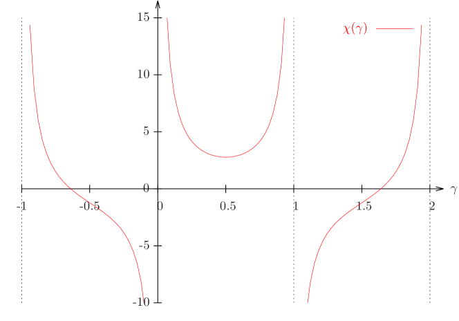
The structure of the function $\chi$ is shown in Fig. 17. It has poles for all integer values of $\gamma$. The branch which gives the main contribution to the solution of the BFKL equation is $\gamma\in]0,1[$. In the complex plane, $\chi$ has actually a saddle-point at $\gamma=\frac{1}{2}$, around which the solution may be expanded for large rapidities.

3.3.2 Compact expression for the BFKL and BK equations

We now aim at writing the BFKL and eventually the BK equations in a more compact way. We use the fact that a linear operator $K_{x}$ acting on some function $u(x)$ may be represented by its eigenvalues. Indeed,

$$K_{x}\cdot u(x)=K_{x}\cdot\int\frac{d\gamma}{2i\pi}e^{\gamma x}\tilde{u}(\gamma)=\int\frac{d\gamma}{2i\pi}\tilde{u}(\gamma)K_{x}\cdot e^{\gamma x}$$ (95)

and if $\chi(\gamma)$ is the eigenvalue of $K_{x}$ which corresponds to the eigenfunction $e^{\gamma x}$, we arrive at a formal expression for the action of $K_{x}$ on the function $u(x)$:

$$K_{x}\cdot u(x)=\int\frac{d\gamma}{2i\pi}\tilde{u}(\gamma)\chi(\gamma)\cdot e^{\gamma x}=\chi(\partial_{x})\int\frac{d\gamma}{2i\pi}\tilde{u}(\gamma)\cdot e^{\gamma x}=\chi(\partial_{x})u(x).$$ (96)

Applying this procedure to the BFKL equation,

$$\partial_{y}T(x_{01},y)=\bar{\alpha}\chi\left(\partial_{\ln|x_{01}|^{2}}\right)T(x_{01},y).$$ (97)

To further analyze the BFKL and BK equations, it proves simpler to go to momentum space by defining

$$\tilde{T}(k,y)=\int\frac{d^{2}x_{01}}{2\pi x_{01}^{2}}e^{ikx_{01}}T(x_{01},y).$$ (98)

The form of the BFKL equation remains essentially unchanged since the Fourier transform is just a change of basis:

$$\partial_{y}\tilde{T}(k,y)=\bar{\alpha}\chi\left(-\partial_{\ln|k|^{2}}\right)\tilde{T}(k,y).$$ (99)

The nonlinear term turns out to drastically simplify in momentum space. Its Fourier transform reads

$$\int\frac{d^{2}x_{01}}{2\pi x_{01}^{2}}e^{ix_{01}k}\left[\bar{\alpha}\int\frac{d^{2}x_{2}}{2\pi}\frac{x_{01}^{2}}{x_{02}^{2}x_{12}^{2}}T(x_{02},y)T(x_{12},y)\right].$$ (100)

One can perform the change of variables in the integrals $(x_{01},x_{2})\rightarrow(x_{21},x_{02})$ to get

$$\bar{\alpha}\int\frac{d^{2}x_{21}}{2\pi x_{12}^{2}}\frac{d^{2}x_{02}}{2\pi x_{02}^{2}}e^{ik(x_{02}+x_{21})}T(x_{02},y)T(x_{12},y)\\ =\bar{\alpha}\int\frac{d^{2}x_{21}}{2\pi x_{12}^{2}}e^{ikx_{21}}T(x_{12},y)\int\frac{d^{2}x_{20}}{2\pi x_{02}^{2}}e^{ikx_{02}}T(x_{02},y).$$ (101)

The two factors are just equal to $\tilde{T}(k,y)$.

All in all, the BK equation reads, in $k$ space

$$\partial_{y}\tilde{T}(k,y)=\bar{\alpha}\chi\left(-\partial_{\ln|k|^{2}}\right)\tilde{T}(k,y)-\bar{\alpha}\left[\tilde{T}(k,y)\right]^{2}.$$ (102)

In this form, we see that this equation looks very much like the FKPP equation (37), except for the linear part which is not a second-order differential operator, but an integral operator (up to changes of variables).

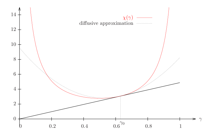
However, this integral operator may be expanded. Indeed, let us perform a Taylor expansion of the kernel eigenvalue $\chi(\gamma)$ around some $\gamma_{0}$:

$$\chi(\gamma)=\chi(\gamma_{0})+(\gamma-\gamma_{0})\chi^{\prime}(\gamma_{0})+\frac{1}{2}(\gamma-\gamma_{0})^{2}\chi^{\prime\prime}(\gamma_{0}).$$ (103)

The expanded kernel is obtained by replacing $\gamma$ by the differential operator $-\partial_{\ln|k|^{2}}$, and thus the BFKL equation becomes a second-order partial differential equation. This is called the “diffusive approximation”. We shall digress on this approximation in connection to the solution to the linear BFKL equation.

3.3.3 Diffusive approximation

If $\gamma_{0}=\frac{1}{2}$, then the diffusive approximation is equivalent to the saddle-point approximation for the solution of the BFKL equation. Recall that the full solution reads

$$T(x_{01},y)=\int\frac{d\gamma}{2i\pi}\tilde{T}(\gamma)|x_{01}|^{2\gamma}e^{\bar{\alpha}\chi(\gamma)y}.$$ (104)

$\tilde{T}(\gamma)$ is the initial condition for the evolution, namely the scattering amplitude at zero rapidity. If $y$ is very large, then the integral is dominated by the saddle point. which is determined by the equation $\left(\bar{\alpha}\chi(\gamma)\right)^{\prime}=0$. The latter is solved by $\gamma=\gamma_{0}=\frac{1}{2}$. One then expands the argument of the exponential to second order around $\gamma_{0}$. After some trivial simplifications, one gets

$$T(x_{01},y)=e^{\bar{\alpha}\chi(\frac{1}{2})y}\int_{\frac{1}{2}-i\infty}^{\frac{1}{2}+i\infty}\frac{d\gamma}{2i\pi}\tilde{T}(\gamma)e^{\frac{\bar{\alpha}}{2}(\gamma-\frac{1}{2})^{2}\chi^{\prime\prime}(\frac{1}{2})y}.$$ (105)

Changing integration variable by writing $\gamma=\frac{1}{2}+i\nu$,

$$T(x_{01},y)=\tilde{T}({\scriptstyle\frac{1}{2}})|x_{01}|e^{\bar{\alpha}\chi(\frac{1}{2})y}\int_{-\infty}^{+\infty}\frac{d\nu}{2\pi}e^{-\frac{\bar{\alpha}}{2}\chi^{\prime\prime}(\frac{1}{2})y\nu^{2}+i\nu\ln|x_{01}|^{2}}.$$ (106)

The remaining integral over $\nu$ is a Gaussian integral. Taking into account the special values of $\chi$

$$\chi({\scriptstyle\frac{1}{2}})=4\ln 2,\ \ \chi^{\prime\prime}({\scriptstyle\frac{1}{2}})=28\zeta(3),$$ (107)

where $\zeta(x)=\sum_{n=1}^{\infty}\frac{1}{n^{x}}$ is the Riemann zeta function, the final result reads

$$T(x_{01},y)=\tilde{T}\left({\scriptstyle\frac{1}{2}}\right)|x_{01}|e^{4\ln 2\bar{\alpha}y}\frac{\exp\left(-\frac{\ln^{2}|x_{01}|^{2}}{56\zeta(3)\bar{\alpha}y}\right)}{\sqrt{56\zeta(3)\pi\bar{\alpha}y}}.$$ (108)

When writing down this formula, we implicitly assume that the transverse distances are expressed in units of the size of the target.

In the case in which $|x_{01}|$ is not too different from 1, namely if one scatters a dipole whose size obeys $|\ln|x_{01}|^{2}|\ll\sqrt{y}$, then the Gaussian factor tends to 1 and $T$ exhibits an exponential growth with the rapidity.

Note that at very large rapidities, $T$ eventually tends to infinity. On the other hand, since $T$ is related to a probability, it should be bounded. The unitarity of $T$ is actually preserved by the BK equation, thanks to the nonlinear term therein. This forces us to consider constant values of $T$, namely to go to a frame which is moving with the rapidity, instead of fixing the dipole size. In this case, the relevant eigenvalue is not $\chi(\frac{1}{2})$ but, as seen before, $\chi(\gamma_{0})$ where $\gamma_{0}$ solves $\chi(\gamma_{0})/\gamma_{0}=\chi^{\prime}(\gamma_{0})$ (see Fig. 18).

Figure 18: Principal branch of the function $\chi(\gamma)$ (red line), graphical solution of the equation $\chi^{\prime}(\gamma_{0})=\chi(\gamma_{0})/\gamma_{0}$ which defines $\gamma_{0}$ (solid black line), and quadratic approximation of $\chi(\gamma)$ around $\gamma=\gamma_{0}$ (dotted black line).

3.3.4 BK in the diffusive approximation and FKPP

We are now in a position to exhibit a rigorous mapping between BK and FKPP. The BK equation reads, in the diffusive approximation

$$\partial_{y}\tilde{T}(k,y)=\bar{\alpha}\left[-\chi^{\prime}(\gamma_{0})\partial_{\ln|k|^{2}}\tilde{T}(k,y)+\frac{1}{2}\chi^{\prime\prime}(\gamma_{0})(\partial_{\ln|k|^{2}}+\gamma_{0})^{2}\tilde{T}(k,y)\right]-\bar{\alpha}\left[\tilde{T}(k,y)\right]^{2}.$$ (109)

One has to perform a mere change of variables in order to get the FKPP equation. We leave the details as an exercise for the reader.

Exercise 7.

Show that the BK equation for $\tilde{T}$ in the diffusive approximation (109) maps exactly to the FKPP equation (37) for $u$ through the change of variables

$$\bar{\alpha}y=\frac{2t}{\gamma_{0}^{2}\chi^{\prime\prime}(\gamma_{0})},\ \ \ln|k|^{2}=\frac{x}{\gamma_{0}}-\frac{2}{\gamma_{0}}\left(1-\frac{\chi^{\prime}(\gamma_{0})}{\gamma_{0}\chi^{\prime\prime}(\gamma_{0})}\right)t,\ \ \tilde{T}(k,y)=\frac{\gamma_{0}^{2}\chi^{\prime\prime}(\gamma_{0})}{2}u(x,t).$$ (110)

Strictly speaking, this mapping holds in momentum space. But it is clear that the physics of the branching random walk is the same in coordinate space. On the practical side, coordinate space is maybe more convenient for model building: $\sigma^{\gamma^{*}p/A}$ is a convolution involving the dipole cross section in coordinate space. On the theoretical side, it is in coordinate space that the unitarity bound can be formulated for $T$.

We expect that all results obtained for $u$ solving the FKPP equation to go over also to the QCD amplitudes in coordinate space, up to the substitution $\ln|k|^{2}\rightarrow\ln 1/|x_{01}|^{2}$.

3.4 Generalization: full BK and FKPP universality class

We have exhibited a rigorous mapping between FKPP and an approximate (diffusive) form of BK. But with some acquaintance with the physics of branching random walks, once a given problem has been identified from general considerations to belong to the class of branching random walks, it is enough to identify the correct space and time variables and the branching-diffusion kernel eigenvalue function in order to be able to conjecture the quantitative asymptotics of the solutions to the equivalent FKPP equation. As for BK, the correspondence is given in Tab. 1.

FKPP		BK
evolution variable $t$	$\longrightarrow$	rapidity $y$
spatial variable $x$	$\longrightarrow$	log of the dipole size $\ln 1/|x_{01}|^{2}$ or of the transverse momentum $\ln|k|^{2}$
branching-diffusion kernel eigenvalues ($\gamma^{2}+1$ for FKPP)	$\longrightarrow$	BFKL eigenvalues $\bar{\alpha}\chi(\gamma)$
Position of the wave front $X(t)$	$\longrightarrow$	log of the saturation scale $\ln Q_{s}^{2}(y)$

Table 1: Dictionary between FKPP and BK.

We shall conjecture that the full BK equation is in the universality class of the FKPP equation. By this we mean that asymptotic results such as (67) may be applied to BK just changing variables/functions as in Tab. 1. However, before we can take over these results obtained for the FKPP universality class, we should examine the shape of the initial condition to understand whether the solution is determined by the shape of the initial condition or if it is solely determined by the dynamics.

Initial condition.

We know that the properties of the solutions to the FKPP equation at large time depend on the shape of the initial condition. We saw that these properties are determined by the dynamics of the branching diffusion process if the initial condition is “steep enough”.

A reasonable ansatz for the scattering of a dipole off a large nucleus at zero rapidity is given by the McLerran-Venugopalan model, which basically assumes an arbitrary number of independent two-gluon exchanges between the dipole and the various nucleons inside the nucleus (see Fig. 19).

Figure 19: One graph contributing to the McLerran-Venugopalan dipole-nucleus amplitude (111). The nucleus is assumed to consist in a large number of independent nucleons, in such a way that the two-gluon exchanges be independent.

The elastic $S$-matrix element in the McLerran-Venugopalan model [MV94a, MV94b] reads

$$S_{\text{MV}}(x_{01})=e^{-\frac{x_{01}^{2}\bar{Q}_{s}^{2}}{4}}$$ (111)

where $\bar{Q}_{s}$ is a momentum scale, the saturation scale of the nucleus. It depends on the gluon density in the nucleons and on the atomic mass number of the nucleus. Expressed in logarithmic scale for the transverse distances and expanded for $|x_{01}|$ small,

$$S_{\text{MV}}(x_{01})=\exp\left(-e^{-\ln\frac{4}{\bar{Q}_{s}^{2}|x_{01}|^{2}}}\right)\simeq 1-e^{-\ln\frac{4}{\bar{Q}_{s}^{2}|x_{01}|^{2}}}$$ (112)

$T_{\text{MV}}=1-S_{\text{MV}}$ has the form $\text{const}\times e^{-\beta x}$, with $x=\ln 1/|x_{01}|^{2}$ and $\beta=1>0.63=\gamma_{0}$. Hence this initial condition is indeed steep enough so that we are in the “pulled front” case.

Note that this feature is more general than the McLerran-Venugopalan model: The fact that the QCD scattering amplitude of a color-neutral object of size $x_{01}$ vanishes as $x_{01}^{2}$ is a fundamental property of QCD known as color transparency.

3.5 Properties of the solutions to the BK equation and models for DIS

3.5.1 Traveling wave property and geometric scaling

Since the BK equation is in the universality class of the FKPP equation, with an initial condition which is “steep enough”, we can take over the results obtained from the FKPP equation to QCD.

The main question we need to address is: What are the QCD traveling waves? Are there phenomenological consequences of their existence? We will then try and use the knowledge on the solutions to the BK equation to build models and fit the data.

We recall that a traveling wave is a solution such that

$${u}(x,t)\underset{t\rightarrow+\infty}{\sim}{\cal U}(x-X^{(\beta)}(t)),$$ (45^′)

where $X(t)$ is the position of the wave front. In general, starting from a given initial condition, the traveling wave appears asymptotically for large $t$.

We now know that $T$ obeys an equation similar to the FKPP equation, with the spatial variable being the logarithm of the dipole size $x\rightarrow\ln|x_{01}|^{2}$, and the evolution variable the rapidity: $t\rightarrow y$. Let us introduce a rapidity-dependent distance $R_{s}(y)$, and the associate momentum $Q_{s}(y)=1/R_{s}(y)$ that we shall call “saturation momentum”.

Then the traveling wave property for the QCD amplitude $T$ reads

$$T(x_{01},y)=T(\ln|x_{01}|^{2}-\ln R_{s}^{2}(y)),$$ (113)

which means that for $y$ very large, $T$ only depends on the product $|x_{01}|^{2}\times Q_{s}^{2}(y)$. This scaling property can be checked for the BK equation in a numerical simulation and is indeed well verified, see Fig. 20.

(a)	(b)

Figure 20: Numerical solution of the BK equation in momentum space, starting from a McLerran-Venugopalan initial condition. (a) Front shape (logarithmic scale) for different rapidities. (b) Reduced front shape in the frame of the wave (logarithmic scale on the $x$-axis). [Plots from Ref. [EGBM05]].

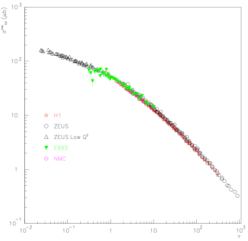
The scaling (113) which should hold for the abstract dipole scattering amplitude actually goes (approximately) over to the DIS cross section, at least when assuming that the quarks are massless. Indeed, taking into account the relation $S=1-T$ and the fact that $S$ is essentially real at high energies, and assuming furthermore that the impact-parameter dependence is constant over a disk of radius $R$ (namely replacing $\int d^{2}b\rightarrow\pi R^{2}$), we rewrite Eq. (73) as

$$\sigma^{\gamma^{*}p/A}(Q^{2},y)=2\pi R^{2}\int d^{2}{x_{01}}dz|\psi^{Q}(x_{01},z)|^{2}T(x_{01},y)$$ (114)

The explicit expression for the photon wave function in quarks reads…

Thus we find that $\sigma^{\gamma^{*}p/A}(Q^{2},y)$ is actually a function of a single variable, namely $Q^{2}/Q_{s}^{2}(y)$. This is called geometric scaling: It is the statement that all DIS data (at small enough $x$) should fall in the same curve when plotted against the scaling variable. This is a prediction which can be tested against the data.

Now the question is what is the $y$-dependence of the saturation scale. We just need to notice that $\ln Q_{s}^{2}(y)$ is the position of the traveling wave. Hence

$$\ln Q_{s}^{2}(y)/\bar{Q}_{s}^{2}=\bar{\alpha}\chi^{\prime}(\gamma_{0})y-\frac{3}{2\gamma_{0}}\ln y+\text{const}$$ (115)

where we introduce the natural scale for $Q_{s}$, namely the saturation scale of the nucleus $\bar{Q}_{s}$. Exponentiating the above equation,

$$Q_{s}^{2}(y)=\bar{Q}_{s}^{2}\frac{e^{\bar{\alpha}\chi^{\prime}(\gamma_{0})y}}{y^{{3}/{2\gamma_{0}}}}\simeq\bar{Q}_{s}^{2}e^{\lambda y}$$ (116)

Thus we see that the saturation momentum grows exponentially with the rapidity at the rate $\lambda=\bar{\alpha}\chi^{\prime}(\gamma_{0})$, up to power corrections. This means that as energy increases, the nucleus becomes less and less transparent also to small dipoles, or, said in another way, absorbs dipoles of smaller and smaller sizes.

As seen in Fig. 21, geometric scaling is a very striking feature of the deep-inelastic scattering data at small $x$.

Figure 21: Inclusive $\gamma^{*}p$ cross section extracted from the deep-inelastic scattering data for $x_{\text{Bj}}<10^{-2}$, plotted against $Q^{2}/Q_{s}^{2}(y)$. All the data fall on the same curve: This is geometric scaling, or equivalently, which may be interpreted as the traveling wave properties of the solution to the BK equation. [Figure from Ref. [MS06]; original plot in Ref. [SGBK01]].

We can also predict the shape of the dipole amplitude from the solutions to (generalized) FKPP equations. From these elements (saturation scale and shape of the amplitude), one can try and build models for the dipole cross section, and apply them to a description of the scattering amplitudes measured in deep-inelastic scattering experiments.

3.5.2 Towards a model for deep-inelastic scattering

In order to arrive at predictions for the DIS cross section, all we need is a model for the $S$-matrix element (see Eq. (73) or, equivalently, for the amplitude $T$, see Eq. (114)) for the forward elastic interaction of a dipole with the target proton or nucleus.

The Golec-Biernat and Wüstoff model [GBW98, GBW99].

The simplest model consists in promoting the saturation scale in the McLerran-Venugopalan model (111) to a function of the rapidity

$$\bar{Q}_{s}^{2}\rightarrow Q_{s}^{2}(y)=\bar{Q}_{s}^{2}e^{\lambda y}$$ (117)

and let $\bar{Q}_{s}$ and $\lambda$ be free parameters. Equation (117) is the leading-order approximation if $\lambda=\bar{\alpha}\chi^{\prime}(\gamma_{0})$ but this expression for $\lambda$ is too crude since it is based on the leading-order BK equation, which is not accurate enough for phenomenology.

Using Eq. (114) with $S$ given by Eq. (111) and the saturation scale therein being replaced by Eq. (117), we obtain the famous Golec-Biernat and Wüstoff model. It has only three free parameters ($R$, $\bar{Q}_{s}$ and $\lambda$), and it turns out that it is able to describe reasonably well all inclusive (and also diffractive) data for deep-inelastic scattering of electron/positron off protons at small $x_{\text{Bj}}\equiv Q^{2}/s$. (By “small” is usually meant $x_{\text{Bj}}\leq 10^{-2}$).

There are several refinements of this model one may think of. The first one would be to build an amplitude whose shape is closer to the shape of the BK traveling waves, as we shall see in the next paragraph. The second one, which we will not discuss in detail here, would be to introduce a more elaborate impact-parameter profile.

Refinements.

Going back to Eq. (67), we perform the changes of variables according to Tab. 1. The dipole scattering amplitude reads, for dipole sizes smaller than the inverse saturation scale

$$T(y,x_{01})\propto\left|\ln\left(|x_{01}|^{2}Q_{s}^{2}(y)\right)\right|\left(|x_{01}|^{2}Q_{s}^{2}(y)\right)^{\gamma_{0}}e^{-\frac{\ln^{2}\left(|x_{01}|^{2}Q_{s}^{2}(y)\right)}{2\bar{\alpha}\chi^{\prime\prime}(\gamma_{0})y}}.$$ (118)

The first two factors exhibit geometric scaling, while the last one, which is different from one whenever $\left|{\ln\left(|x_{01}|^{2}Q_{s}^{2}(y)\right)}\right|$ is not small with respect to $\sqrt{2\bar{\alpha}\chi^{\prime\prime}(\gamma_{0})y}$, encodes geometric scaling violations at finite rapidity $y$ since it exhibits an explicit $y$ dependence. As already mentioned, this formula is valid for small enough dipole sizes, hence in the “dilute” regime where $T\ll 1$. To construct the full amplitude, we also need to understand the properties of $T$ in the saturation regime, where $T\sim 1$ or $S\ll 1$ To this aim, we go back to the BK equation for $S$ given in Eq. (77), and rewrite it in this limit, in which the nonlinear term $S(y,x_{02})S(y,x_{12})$ can be neglected:

$$\partial_{y}S(y,x_{01})=\bar{\alpha}\int_{1/Q_{s}^{2}(y)}\frac{d^{2}x_{2}}{2\pi}\frac{x_{01}^{2}}{x_{02}^{2}x_{12}^{2}}\left[-S(y,x_{01})\right].$$ (119)

The lower bound on the integral means that both $|x_{02}|$ and $|x_{12}|$ have to be larger than $1/Q_{s}(y)$, which is the condition for the equation to linearize. Now the $S$ factor goes out of the integral since it has no $x_{2}$ dependence, and the dominant contribution to the latter comes from the two collinear regions $|x_{02}|,|x_{12}|\ll|x_{01}|$

$$\int_{1/Q_{s}^{2}(y)}\frac{d^{2}x_{2}}{2\pi}\frac{x_{01}^{2}}{x_{02}^{2}x_{12}^{2}}\simeq 2\int_{1/Q_{s}^{2}(y)}^{x_{01}^{2}}\frac{d^{2}x_{2}}{2\pi}\frac{1}{x_{02}^{2}}=\ln(|x_{01}|^{2}Q_{s}^{2}(y)).$$ (120)

We may then integrate the differential equation from some initial rapidity $y_{0}$ to $y$:

$$S(y,x_{01})=S(y_{0},x_{02})e^{-\bar{\alpha}\int_{y_{0}}^{y}dy^{\prime}\,\ln(|x_{01}|^{2}Q_{s}^{2}(y^{\prime}))}.$$ (121)

We leave the final integration as an exercise.

Exercise 8.

Knowing the expression for $Q_{s}(y)$ (keep only the leading term), complete the calculation by integrating over $y^{\prime}$.
The final result is known as the “Levin-Tuchin law” [LT00]. A refined version of this calculation has come out very recently, see [CLM14].

Now we may try and match the two expressions (118) and (121): We get the IIM model [IIM04], which successfully describes the HERA data.

   Intermediate recap
Parton evolution in the high-energy of QCD is a peculiar branching random walk. The Balitsky-Kovchegov equation (78), which drives the energy evolution of QCD scattering amplitudes, is in the universality class of the FKPP equation (37). It turns out that there is an exact mapping in the diffusive approximation for the kernel of the BK equation, but more generally, one can argue that the asymptotics of the two equations should be identical up to the identification of the relevant variables. Properties of the solutions to the BK equation can be inferred from what is known on the solutions to the FKPP equation, leading to the expression (118) for the scattering amplitude, and (116) for the saturation scale. The traveling wave property corresponds to geometric scaling, which was found in the deep-inelastic scattering data (Fig. 21). $\blacksquare$   

To go further
One limit which was taken to arrive the BK evolution equation is the large-number of color ($N_{c}$) limit. An equation which takes into account finite-$N_{c}$ corrections is known: It is the so-called Jalilian-Marian-Iancu-McLerrran-Leonidov-Kovner (JIMWLK) equation, see Ref. [ILM01, FILM02] and references therein. Numerical solutions of the latter [RW04] seem to show that its solutions are very similar to the solutions to the BK equation. But we shall cautiously deem that the question whether the JIMWLK equation contains the same physics as the BK equation is still an open question.

High-energy QCD, the dipole model and the BK equation were introduced in Prof. Mueller’s lectures at Wuhan’s school. For more, see the original paper [Mue94] and the recent textbook of Ref. [KL12].

4 Beyond the simple branching random walk – Beyond the Balitsky-Kovchegov equation

So far, we have considered that gluons evolve through $\text{gluon}\rightarrow\text{gluon}+\text{gluon}$ splittings only, and we have neglected the correlations of multiple gluons in the course of partonic evolution. However, QCD would a priori also allow for gluon recombinations, and further color charge interactions. One expects these processes to play a role when the density becomes large enough. While this has not been properly formulated in QCD, we may introduce such recombination/saturation processes in branching random walks, and obtain modified evolution equations for e.g. the particle density. It turns out that the solutions to these equations have universal features which are independent of the details of the recombination processes. This is what we will be after in this section.

4.1 Motivation

Deep-inelastic scattering at high energies may be seen as a dipole-target interaction process, once the virtual photon wave function in $q\bar{q}$ pairs has been factorized. The simplest model for each of the nucleons in the target is a color dipole.

The lowest order contribution to the dipole-dipole elastic scattering amplitude is given by the two-gluon exchange graphs (see Fig. 22).

$+$

$+$

$+$

$+\ \text{[sym.]}\equiv$

Figure 22: Graphs contributing to the scattering of two color dipoles (at zero rapidity; see Eq. (123)) and the graphical representation of their sum that we shall use later.

The interaction is local in impact parameter, in the sense that dipoles which have no geometric overlap, namely whose centers do not sit within a distance smaller than the size of say the largest dipole, interact very weekly. The amplitude for the scattering of dipoles of respective sizes $r$ and $r_{0}$ sitting on top of each other in transverse space approximately reads

$$T_{\text{el}}(r,r_{0})\simeq\alpha_{s}^{2}\frac{r_{<}^{2}}{r_{>}^{2}},$$ (122)

where $r_{<}=\min(r,r_{0})$ and $r_{>}=\max(r,r_{0})$. In logarithmic coordinates, we can consider that this is a local interaction also in the dipole sizes and replace $T_{\text{el}}$ by

$$T_{\text{el}}(r,r_{0})\simeq\alpha_{s}^{2}\delta(\ln r^{2}/r_{0}^{2}).$$ (123)

QCD evolution replaces an initial dipole of size $x_{01}$ by a density $n(r,y|x_{01})$ of dipoles of size $r$ at rapidity $y$ (see Fig. 23).

(a)	(b)

Figure 23: (a) Example of dipole graph contributing to dipole-dipole scattering in the restframe of the lower dipole (the so-called “target”), and whose sum is represented by the BFKL equation. There is a single two-gluon exchange, represented by the red vertical line. (b) At higher rapidity, multiple two-gluon exchanges may occur and, if the target is a single dipole, the interactions are no longer independent. This case has not been formulated in a satisfactory way yet.

Let us assume for a moment that the target is a single dipole of size $r_{0}$. Then the amplitude reads

$$T(x_{01},y)=\int\frac{dr^{2}}{r^{2}}T_{\text{el}}(r,r_{0})\int dP[n]n(r,y|x_{01}),$$ (124)

where $dP[n]$ is a formal notation for the probability of a dipole configuration of density $n$. The last integral just gives the mean density of dipoles of size $r$. Using Eq. (123) to perform the integral over $r^{2}$, we arrive at the formula

$$T({x_{01},y})\simeq\alpha_{s}^{2}\langle n(r_{0},y|x_{01})\rangle.$$ (125)

This formula says that the scattering amplitude is proportional to the average number of dipoles of size which matches the size $r_{0}$ of the target after evolution of the projectile of initial size $x_{01}$ over $y$ units of rapidity. We know that the mean density of dipoles grows like the exponential of the rapidity: $\langle n(r_{0},y)\rangle\sim e^{\bar{\alpha}y}$. Hence when $\bar{\alpha}y\geq\bar{\alpha}y_{\text{sat}}\equiv\ln(1/\alpha_{s}^{2})$, $T$ becomes larger than 1. But $T$ can be interpreted as the probability that a dipole in the Fock state of the projectile interact with the target, and thus should be less than unity throughout the evolution. Actually, this means that the approximation in which there is only one elementary interaction (in which the BFKL equation is justified) breaks down at $y\sim y_{\text{sat}}$, and one should take into account multiple exchanges (see Fig. 23b).

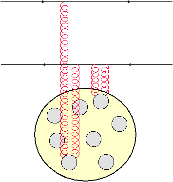
If the target is a very large nucleus instead of a single dipole, then these interactions are all independent (see Fig. 24), since combinatorially, the probability that two interactions occur with the same nucleon is small. In this case, one should simply replace Eq. (125) by the BK equation with the appropriate initial condition representing the scattering of an elementary dipole of size $x_{01}$ with a set of dipoles of size $r_{0}$. This is the McLerran-Venugopalan model.

(a)	(b)

Figure 24: (a) Example of dipole graph contributing to dipole-nucleus scattering at zero rapidity. Such graphs are resummed by the McLerran-Venugopalan formula. (b) When the upper dipole is boosted, it interacts through quantum fluctuations. The corresponding graphs are resummed by the BK equation.

If however the target is a single dipole, then the interactions are necessarily correlated and the BK equation is a priori not justified (although, as we will see later, its solution may represent correctly the physics of dipole-dipole scattering for low enough rapidity), as seen in Fig. 23b.

Let us go back to the BFKL evolution in order to estimate roughly at which rapidity the BFKL description is expected to break down in dipole-dipole scattering.

	$n(y)$ 1		$n({\scriptstyle\frac{y}{2}})$ $n({\scriptstyle\frac{y}{2}})$		$1$ $n(y)$
(a)		(b)		(c)

Figure 25: BFKL evolution viewed in different frames. (a) Restframe of the lower dipole, (b) center-of-mass frame where the rapidity is equally shared between the dipoles, (c) resframe of the upper dipole. The average number of dipoles in each of the objects depends on the rapidity and on the frame, and is indicated in the figure.

The answer actually depends on the frame (see Fig. 25). In the restframe of one or of the other dipole, the scattering amplitude is roughly given by Eq. (125), namely $T(y)\sim\alpha_{s}^{2}\langle n(y)\rangle$ (we kept only the $y$ dependence in this equation). $T$ should be less than one for the BFKL equation to apply, which means that the number of dipoles should be effectively less than $1/\alpha_{s}^{2}$ for the dipole evolution being linear, namely for it being an ordinary branching random walk.

We already recalled that the dipole number grows exponentially with $\bar{\alpha}y$. This gives a maximum rapidity for the dipole evolution to be linear in the laboratory frame equal to

$$Y_{\text{lab}}\sim y_{\text{sat}}=\frac{1}{\bar{\alpha}}\ln\frac{1}{\alpha_{s}^{2}}.$$ (126)

We dropped uninteresting constants.

In the center-of-mass frame instead, the amplitude reads $T(y)\sim\alpha_{s}^{2}\langle n({\scriptstyle\frac{y}{2}})\rangle\langle n({\scriptstyle\frac{y}{2}})\rangle$, leading to a different expression for the maximum rapidity for the dipole evolution being linear:

$$Y_{\text{com}}\sim\frac{2}{\bar{\alpha}}\ln\frac{1}{\alpha_{s}^{2}}=2Y_{\text{lab}}.$$ (127)

But of course, for $y=Y_{\text{com}}$, the overall amplitude $T(y)$ would be larger than one, and so multiple scatterings must occur (see Fig. 26a). Since the dipoles are correlated, the evolution of the amplitude cannot be described by the BK equation.

(a)	(b)

Figure 26: (a) Example of dipole graph contributing to dipole-dipole scattering at rapidity $\frac{1}{\bar{\alpha}}\ln\frac{1}{\alpha_{s}^{2}}<y<\frac{2}{\bar{\alpha}}\ln\frac{1}{\alpha_{s}^{2}}$ in the center-of-mass frame. In this regime, the dipole wave functions evolve according to linear dipole evolution, but the total amplitude is in the saturation regime and multiple exchanges are needed in order to unitarize the amplitude. (b) The same boosted to the lab frame (restframe of the target dipole). Now one expects nonlinear interactions in the course of the evolution of the projectile dipole.

Hence a proper formulation of dipole-dipole scattering seems to require the introduction of a nonlinear mechanism in the evolution itself which would effectively limit the density of dipoles to $\sim 1/\alpha_{s}^{2}$. How to do this is not known yet. However, we may try and understand the effects of these nonlinearities starting with a simple branching random walk supplemented with recombinations, and then figure out what is universal and thus what may be taken over to QCD.

4.2 BRW with selection/recombination: stochastic traveling waves

4.2.1 A simple model with stochastic traveling wave for Darwinian population evolution

We have already introduced a model for population evolution in Sec. 2.5 as an example of branching-diffusion process. We had a population of individuals, each characterized by the “fitness” $x$, a real number. The time evolution of the population was defined by the following rule (see Fig. 27):

Figure 27: Elementary processe defining the evolution of each individual in the population from generation $g$ to $g+1$.

Each individual with fitness $x$ present in the population at generation number $g$ is replaced at the next generation $g+1$ by two offspring, which have respective fitnesses $x_{1}$ and $x_{2}$ such that

$$x_{1}=x+\varepsilon_{1},\ x_{2}=x+\varepsilon_{2},$$ (70’)

where $\varepsilon_{1},\varepsilon_{2}$ are random numbers distributed according to a probability distribution $\rho(\varepsilon)$. One now adds another rule for the evolution: Whenever the total population reaches some integer $N$, for the further evolution, one removes from the population the least “fit” individuals in such a way as to always keep the population size constant and equal to $N$. This is a selection mechanism, and our model is now a simple model for Darwinian population evolution. Indeed, the fitness is inherited by the offspring, up to stochastic variations which represent the mutations. The selection mechanism enforces the fact that only the fittest survive.

Realizations of such a model are represented in Fig. 28, in the case of a small population ($N=10$, Fig. 28a) and also for a larger population ($N=200$, Fig. 28b). A function which exhibits traveling wave properties is $h_{g}(x)$, the fraction of individuals which have a fitness larger than $x$ at generation $g$.

(a)	(b)

Figure 28: One realization of the population evolution model, for different population sizes: (a) $N=10$, (b) $N=200$. In each case, the fitnesses of the individuals are represented for 5 generations. The links indicate the genealogy. The curves at the bottom of the figure represent the fraction $h_{g}(x)$ of individuals which have fitness larger than $x$ at generation $g$. (Arbitrary scale on the $x$-axis.)

We can make a few remarks looking at Fig. 28. First, we see that the dispersion in fitness of the population remains of the same order of magnitude throughout the evolution and its mean increases. These features are of course due to the selection mechanism. We also see that when the population increases, the curves representing $h_{g}(x)$ look smoother: The noise gets averaged due to the large number of objects (see Fig. 28b). But actually, the stochasticity always remains significant in the low-density tip of the front.

4.2.2 Reaction-diffusion model

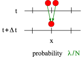
Let us come back to our branching random walk process on a lattice introduced in Sec. LABEL:sec:introBRW. We shall just add a recombination process: Any pair of particles on site $x$ recombines to one single particle with probability $\lambda/N$, where $N$ is a new parameter (see Fig. 29). This is a reaction-diffusion model, which may apply to the context of chemical reactions or of the spread of diseases.

Ordinary Brownian motion		Branching	Recombination

Figure 29: Elementary processes defining the reaction-diffusion model.

The evolution equation for the average number of particles on site $x$ as time $t$ increases is easy to obtain. We assume a configuration $n(x,t)$ of particles at time $t$, and write the equation for the average $\langle n\rangle$ at time $t+\Delta t$ knowning the configuration at time $t$:

$$\langle n(x,t+\Delta t)\rangle_{[t,t+\Delta t]}=\left(1-2\mu+\lambda\right)n(x,t)+\mu\left[n(x+\Delta x,t)+n(x-\Delta x,t)\right]\\ -\frac{\lambda}{N}n(x,t)\left[n(x,t)-1\right].$$ (128)

The first term in the right-hand side accounts for the mean fraction $2\mu$ of particles which leave the site $x$ due to diffusion and the mean fraction $\lambda$ which are added due to particle splittings. The second term is a gain term due to diffusion from the nearby sites. The last term is the mean number of particles which disappear due to recombination.

We now average over the full history of the stochastic process which leads to the configuration $n(x,t)$

$$\langle n(x,t+\Delta t)\rangle-\langle n(x,t)\rangle=\mu\left[\langle n(x+\Delta x,t)\rangle+\langle n(x-\Delta x,t)\rangle-2\langle n(x,t)\rangle\right]\\ +\lambda\langle n(x,t)\rangle-\frac{\lambda}{N}\langle n(x,t)[n(x,t)-1]\rangle.$$ (129)

In order to get a partial differential equation, we take the continuum limit

$$\Delta t\rightarrow 0,\ \ \Delta x\rightarrow 0\ \ \text{with}\ \ \mu\frac{(\Delta x)^{2}}{\Delta t}=1,\ \ \lambda=\Delta t,$$ (130)

and we arrive at

$$\partial_{t}\langle n\rangle=\partial_{x}^{2}\langle n\rangle+\langle n\rangle-\frac{1}{N}\langle n(n-1)\rangle.$$ (131)

We observe that this is not a closed equation since the right-hand side has a term of the form $\langle n^{2}\rangle$. The most strightforward way to arrive at a closed equation is to assume the factorization of this correlator: $\langle n^{2}\rangle=\langle n\rangle^{2}$. This is a mean-field approximation: It consists in neglecting the fluctuations. It is expected to be a good approximation when the number of particles gets large. The above equation then boils down to

$$\partial_{t}\langle n\rangle=\partial_{x}^{2}\langle n\rangle+\langle n\rangle-\frac{1}{N}\langle n\rangle^{2},$$ (132)

where we have also neglected a term of order $1/N$.

Defining the rescaled mean particle number $u\equiv\langle n\rangle/N$, we arrive at

$$\partial_{t}u=\partial_{x}^{2}u+u-u^{2},$$ (37’)

which is of course again the FKPP equation.

To go further
The full evolution equation for $n$ would be a stochastic partial differential equation with a complicated noise term. There is an elegant formulation of reaction-diffusion processes in terms of a partial differential equation with Gaussian multiplicative noise (see e.g. Ref. [Pel85]), but it requires the introduction of an abstract “field” $\phi(x,t)$ of coherent states. (The moments of $\phi$ are related to the factorial moments of $n/N$). $\phi$ solves an equation of the form

$$\partial_{t}\phi=\partial_{x}^{2}\phi+\phi-\phi^{2}+\sqrt{\frac{1}{N}\phi(1-\phi)}\,\nu,$$ (133)

where the field $\nu$ is a Gaussian white noise, defined by the correlators

$$\langle\nu(x,t)\rangle=0,\ \langle\nu(x,t)\nu(x^{\prime},t^{\prime})\rangle=\delta(x-x^{\prime})\delta(t-t^{\prime}).$$ (134)

One should specify that Eq. (133) has to be understood in the It$\bar{\text{o}}$ sense (see e.g. Ref. [Gar04]).

4.3 Properties of stochastic traveling waves

Insight into stochastic traveling waves was developed in Refs. [BD97] and [BDMM06a]. Since our presentation here is rather concise, we refer the reader to those papers for details and to the review paper of Ref. [Mun09].

4.3.1 General considerations

We first need to gain some intuition on stochastic traveling waves. Thinking of the reaction-diffusion model on a lattice, it is clear that in bins in which the number of particles is large, the evolution is essentially deterministic, hence given by the corresponding equation in the FKPP universality class. We expect the noise to be important only in bins in which the number of particles is of order unity. So if $N$ is large, the mean-field approximation (i.e. the FKPP equation) should have some validity, yet to be understood.

We observe that the main important property of stochastic fronts which is missed when going to the infinite-$N$ limit is the fact that the number of particles on each lattice site is not a continuous variable, but takes integer values, $0,1,2,\cdots$. In particular, starting with a localized initial condition, there must be a rightmost and a leftmost occupied site. So the exponential shape of the front which solves asymptotically (for large times) the FKPP equation, $u(x,t)\sim e^{-(x-X(t))}$, cannot represent the (normalized) number of particles in a given realization. The problem is most stringent in regions in which $u(x,t)<1/N$ (i.e. in which the number of particles $n=N\times u$ would become a fraction of unity if it solved the deterministic FKPP equation).

From this remark, we may first try and guess the velocity of the front describing the particle density in individual realizations, and eventually figure out a method of taking into account discreteness.

We recall that in the (generalized) FKPP case, the front velocity is tightly connected to its shape. Starting from a localized initial condition, it reads

$$\dot{X}(t)=\chi^{\prime}(\gamma_{0})-\frac{3}{2\gamma_{0}t},$$ (135)

and this actually is the velocity of a front whose exponential shape $e^{-\gamma_{0}(x-X(t))}$ extends over a region of size $\sim\sqrt{\chi^{\prime\prime}(\gamma_{0})t}$ (see the Gaussian factor in Eq. (67)). We have just argued that the exponential shape cannot be correct when $u<1/N$. So the front must have a size $L$ which is such that $u(X(t)+L,t)=1/N$, which, taking into account the fact that its shape is exponential, gives

$$L=\frac{1}{\gamma_{0}}\ln N.$$ (136)

Starting from a steep initial condition, the time $t_{\text{diffusion}}$ at which the exponential shape extends over the full allowed range $L$ is of order $L^{2}/\chi^{\prime\prime}(\gamma_{0})$ (see again Eq. (67)), and at that time, from Eq. (135), the front velocity reads

$$\chi^{\prime}(\gamma_{0})-\text{const}\times\frac{3\chi^{\prime\prime}(\gamma_{0})}{2\gamma_{0}L^{2}}.$$ (137)

After this time, the front cannot extend any further, and so this should also be, on the average, the asymptotic front velocity at large time. The constant cannot be determined from this naive estimate, but the parametric form should be correct.

Note that with respect to the asymptotic velocity of the deterministic FKPP front ($\chi^{\prime}(\gamma_{0})$), the correction scales like $1/\ln^{2}N$. Naively, one would have expected a correction of the order of $1/N$ since taking into account discreteness amounts to cutting off a fraction $1/N$ of the tail of the front. The correction we have just argued is much larger!

Figure 30: Left: Front velocity as a function of time for a particular realization of the reaction-diffusion model. Right: Reduced front shape in the frame of the wave for the same realization, at two different times. For $t\ll\ln^{2}N$, we see that the reduced front shape is consistent with e.g. Eq. (60) while at larger $t$, the shape starts to look more symmetric and large fluctuations occur at the tip.

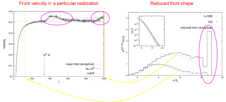
Support for the scenario just outlined can be found in numerical simulations. Figure 30 (left) represents the velocity of the front in one particular realization of the simulation of a reaction-diffusion model (for all details, see Ref. [EGBM05]). We see that indeed, at some time $t\sim\ln^{2}N\sim t_{\text{diffusion}}$, the increase of the front velocity seems to stop, and except for small-amplitude short-term noise and for large but rare upward jumps, the velocity becomes constant. It also seems that when one reaches this “constant” velocity, the shape of the reduced front (namely the front divided by the exponential $e^{-\gamma_{0}x}$, Fig. 30 (right)) departs from the shape predicted by the FKPP equation, see Eq. (60).

We are going first to set up a precise calculation of the average front velocity, and then come back to the large positive fluctuations in the velocity.

4.3.2 Accounting for saturation and discreteness

The simplest way to account for the fact that $u$ cannot exhibit the exponential shape $e^{-\gamma_{0}x}$ in regions in which $u<1/N$ is to put an appropriate cutoff, namely an absorptive boundary, in the tail.

To solve the FKPP equation, we already had an absorptive boundary instead of the nonlinearity. Now we need a second cutoff to represent discreteness. Since the asymptotic front has a length $L$, the second cutoff sits at a fixed distance $L$ of the first one. In between, the evolution equation is linear and deterministic.

Hence we want to solve the linear equation

$$\partial_{t}u=\partial_{x}^{2}u+u$$ (138)

with the two boundary conditions

$$u(X(t),t)=0,\ \ u(X(t)+L,t)=0,$$ (139)

and some localized initial condition. (Its precise form is not relevant since it turns out that it will be “forgotten” after a sufficiently large time). An appropriate ansatz is

$$u(x,t)=e^{-\xi}h\left(\frac{\xi}{L},\frac{t}{L^{2}}\right)$$ (140)

where $\xi=x-X(t)$. Indeed, we know that the dominant shape of the front is a decreasing exponential, that is why we factorized $e^{-\xi}$. Furthermore, the natural distance scale in the problem is $L$, and the natural time scale is the diffusion time over such a distance, namely $L^{2}$. Let us introduce the dimensionless variables $\rho\equiv\xi/L$ and $\tau\equiv t/L^{2}$. Then, in terms of these new variables,

$$\begin{split}\partial_{t}u&=\left[\dot{X}\left(h-\frac{1}{L}\partial_{\rho}h\right)+\frac{1}{L^{2}}\partial_{\tau}h\right]e^{-\xi}\\ \partial_{x}u&=\left[-h+\frac{1}{L}\partial_{\rho}h\right]e^{-\xi}\\ \partial_{x}^{2}u&=\left[h+\frac{1}{L^{2}}\partial_{\rho}^{2}h-\frac{2}{L}\partial_{\rho}h\right]e^{-\xi},\end{split}$$ (141)

hence

$$\partial_{\tau}h=\partial_{\rho}^{2}h+L(\dot{X}-2)\partial_{\rho}h+L^{2}(2-\dot{X})h.$$ (142)

In order to have a nontrivial stationary solution ($\partial_{\tau}h=0$), we need to make sure that the terms proportional to $h$ and $\partial_{\rho}^{2}h$ have a coefficient of order one. Recall that $L$ is a large parameter: We must thus set $\dot{X}=2-\frac{c^{2}}{L^{2}}$ where $c$ is an undetermined constant so far. Then, the term proportional to $\partial_{\rho}h$ becomes negligible. Equation (142) boils down to

$$\partial_{\tau}h=\partial_{\rho}^{2}h+c^{2}h.$$ (143)

A stationary solution obviously solves the second-order differential equation

$$\partial_{\rho}^{2}h+c^{2}h=0,$$ (144)

whose solution reads (for $c>0$)

$$h(\rho,\tau)=A\sin c\rho+B\cos c\rho,$$ (145)

where $A$ and $B$ are arbitrary constants. Compatibility with the boundary conditions (139) requires $c=\pi$ and $B=0$.

Going back to the initial variables, we have thus found

$$u(x,t)\propto e^{-(x-X(t))}\ln N\sin\left[\frac{\pi}{\ln N}\left(x-X(t)\right)\right],\ \ \text{where}\ \ X(t)=\left(2-\frac{\pi^{2}}{\ln^{2}N}\right)t.$$ (146)

Now for a generic model whose branching diffusion kernel is characterized by the eigenvalue $\chi(\gamma)$:

$$u(x,t)\propto e^{-\gamma_{0}(x-X(t))}\frac{\ln N}{\gamma_{0}}\sin\left[\frac{\pi\gamma_{0}}{\ln N}\left(x-X(t)\right)\right],\ \text{where}\ \ X(t)=V_{\text{BD}}t,$$ (147)

and we introduced the front velocity

$$V_{\text{BD}}\equiv\chi^{\prime}(\gamma_{0})-\frac{\pi^{2}\chi^{\prime\prime}(\gamma_{0})}{2\gamma_{0}L^{2}},\ \text{where}\ L=\frac{1}{\gamma_{0}}\ln N.$$ (148)

(The subscript “BD” stands for “Brunet-Derrida”). As before, $L$ is the size of the front, namely in the calculation, up to an additive constant, the distance between the two absorptive boundaries.

4.3.3 Beyond the deterministic equations: modeling noise at the tip

So far, we have replaced the stochastic evolution equation by a deterministic equation with two cutoffs: one for unitarity, ensuring that $n\leq N$, the other one for discreteness, ensuring, in some sense that $n\geq 1$, or more precisely, that $n$ represents indeed a number of particles. Now the full problem is stochastic. Finite-$N$ corrections should reflect more precisely the stochasticity. The question we shall address in this paragraph is how to go beyond the Brunet-Derrida cutoff.

We know that stochasticity plays a role in the tail, where the density of particles is low. Our basic assumption is that the first correction beyond the cutoff, which in some way enforces discreteness, is well represented by a single particle randomly sent a distance $\delta$ ahead of the deterministic tip of the front, at a rate $p(\delta)d\delta$. Except for this stochastic process, all evolution is assumed to be deterministic. In particular, once this particle is randomly produced, its further time evolution is purely deterministic.

Let us imagine that a fluctuation occurs at time $t$. The position of the tip at $t$ is

$$X_{\delta}(t)=X(t)+\delta,$$ (149)

and at later time $t+\Delta t$, after the fluctuation has evolved into a front,

$$X_{\delta}(t+\Delta t)=X_{\delta}(t)+V_{\text{BD}}\Delta t-3\ln L.$$ (150)

The last negative term is a “delay” induced by the formation of the front, and due to the fact that until times of the order of $\Delta t\sim L^{2}$, the front velocity differs from $V_{\text{BD}}$ by $-3/(2\Delta t)$. The front without fluctuation has just translated by $V_{\text{BD}}\Delta t$:

$$X_{\delta}(t+\Delta t)=X(t)+V_{\text{BD}}\Delta t.$$ (151)

Now the shape of the front in the forward part is essentially exponential. The front after the fluctuation has relaxed (at time such that $\Delta t\gg L^{2}$) is the sum of the front without fluctuation translated at time $t+\Delta t$ at the constant velocity $V_{\text{BD}}$, and the front originated from the fluctuation:

$$\begin{split}e^{-(x-X_{\text{tot}}(t+\Delta t))}&=e^{-(x-X(t+\Delta t))}+Ce^{-(x-X_{\delta}(t+\Delta t))}\\ &=e^{-(x-X(t)-V_{\text{BD}}\Delta t)}\left(1+Ce^{\delta-3\ln L}\right).\end{split}$$ (152)

We find that the position of the front with the fluctuation reads

$$X_{\text{tot}}(t+\Delta t)=X(t)+V_{\text{BD}}\Delta t+R(\delta),\ \ \text{where}\ \ R(\delta)\equiv\ln\left(1+C\frac{e^{\delta}}{L^{3}}\right).$$ (153)

$R(\delta)$ just introduced is the additional shift of the front position induced by a forward fluctuation.

In order to be able to compute the effect of these fluctuations, we still need to know the rate at which the forward fluctuations occur, and their distribution in $\delta$. It is natural to assume that the latter is exponential $e^{-\delta}$, and thus we shall conjecture the rate

$$p(\delta)d\delta=C_{1}e^{-\delta}d\delta,$$ (154)

where $C_{1}$ is an unknown constant.

With these elements, we can write the following effective theory for the evolution of $X(t)$:

$$X(t+\Delta t)=\begin{cases}X(t)+V_{\text{BD}}\Delta t&\text{probability}\ \ 1-\Delta t\int_{0}^{+\infty}d\delta\,p(\delta)\\ X(t)+V_{\text{BD}}\Delta t+R(\delta)&\text{probability}\ \ \Delta t\,d\delta\,p(\delta).\end{cases}$$ (155)

The generating function for the cumulants of $X(t)$ is defined by

$$G(\lambda,t)=\ln\left\langle e^{\lambda X(t)}\right\rangle.$$ (156)

Let us write its time evolution:

$$\begin{split}G(\lambda,t+\Delta t)&=\ln\left\langle e^{\lambda X(t+\Delta t)}\right\rangle\\ &=\begin{multlined}\ln\left\langle\left[\Delta t\int_{0}^{+\infty}d\delta\,p(\delta)e^{\lambda\left(X(t)+V_{\text{BD}}\Delta t+R(\delta)\right)}\right.\right.\\ \left.\left.+\left(1-\Delta t\int_{0}^{+\infty}d\delta\,p(\delta)\right)e^{\lambda\left(X(t)+V_{\text{BD}}\Delta t\right)}\right]\right\rangle\end{multlined}\ln\left\langle\left[\Delta t\int_{0}^{+\infty}d\delta\,p(\delta)e^{\lambda\left(X(t)+V_{\text{BD}}\Delta t+R(\delta)\right)}\right.\right.\\ \left.\left.+\left(1-\Delta t\int_{0}^{+\infty}d\delta\,p(\delta)\right)e^{\lambda\left(X(t)+V_{\text{BD}}\Delta t\right)}\right]\right\rangle\\ &=\ln\left\langle e^{\lambda X(t)}\right\rangle+\lambda V_{\text{BD}}\Delta t+\ln\left[1+\Delta t\int_{0}^{+\infty}d\delta\,p(\delta)\left(e^{\lambda R(\delta)}-1\right)\right].\end{split}$$ (157)

The average over the processes occurring in the time interval $[t,t+\Delta t]$ is done using the rules (155), applied to go from the first to the second line. The remaining brackets $\langle\cdot\rangle$ represent the average over the time interval $[0,t]$.

The first term in the right-hand side of the previous equation is, by definition, nothing but $G(\lambda,t)$. Now we take the $\Delta t\rightarrow 0$ limit, in which we can expand the logarithm in the last term and write $G(\lambda,t+\Delta t)=G(\lambda,t)+\Delta t\,\partial_{t}G(\lambda,t)$. We arrive at the equation

$$\frac{\partial G(\lambda,t)}{\partial t}=\lambda V_{\text{BD}}+\int_{0}^{+\infty}d\delta\,p(\delta)\left(e^{\lambda R(\delta)}-1\right),$$ (158)

which is trivial to integrate. One expands the result in powers of $\lambda$ to get the cumulants of $X(t)$. For large $t$ (which enables us to neglect the unknown integration constant),

$$\begin{split}\frac{\left\langle\left[X(t)\right]^{n}\right\rangle_{c}}{t}&=\delta_{n,1}V_{\text{BD}}+\int_{0}^{+\infty}d\delta\,p(\delta)\left[R(\delta)\right]^{n}\\ &=\delta_{n,1}V_{\text{BD}}+C_{1}\int_{0}^{+\infty}d\delta\,e^{-\delta}\ln^{n}\left(1+C\frac{e^{\delta}}{L^{3}}\right).\end{split}$$ (159)

The integral over $\delta$ is performed by the change of variable $\delta\rightarrow x\equiv L^{3}e^{-\delta}/C$:

$$\begin{split}C_{1}\int_{0}^{+\infty}d\delta\,e^{-\delta}\ln^{n}\left(1+C\frac{e^{\delta}}{L^{3}}\right)&=\frac{CC_{1}}{L^{3}}\int_{0}^{L^{3}/C}dx\,\ln^{n}\left(1+\frac{1}{x}\right)\\ &=\frac{CC_{1}}{L^{3}}n!\zeta(n)+{\cal O}(1/L^{6}),\end{split}$$ (160)

where $\zeta(n)$ is the Euler Zeta function. Note that the large-$L$ expansion in the last line can be performed only for $n\geq 2$.

Keeping the leading term when $L\gg 1$ (which is obtained simply by setting the upper bound of the integral over $x$ to $+\infty$), we get

$$\frac{\left\langle\left[X(t)\right]^{n}\right\rangle_{c}}{t}=CC_{1}n!\zeta(n)\frac{1}{L^{3}}.$$ (161)

$CC_{1}$ is an overall constant, the same for all cumulants.

We need to address the case $n=1$ (first moment of $X(t)$) separately, since in this case, the integral over $x$ is logarithmic and thus the upper bound cannot be sent to infinity:

$$\frac{\langle X(t)\rangle}{t}=V_{\text{BD}}+\frac{CC_{1}}{L^{3}}\int_{0}^{L^{3}/C}dx\,\ln\left(1+\frac{1}{x}\right).$$ (162)

The integral is easy to perform. In the limit of large $L$, the leading term just reads $\ln(L^{3})$, in such a way that

$$\frac{\langle X(t)\rangle}{t}=V_{\text{BD}}+{CC_{1}}\frac{3\ln L}{L^{3}}.$$ (163)

The constant $CC_{1}$ appears also here.

We still need to determine this constant. We have not found a way to compute it, but we can try and guess it. For completeness, let us briefly sketch the argument.

We write the expression for the mean displacement rate of the front due to fluctuations only:

$$\int d\delta p(\delta)R(\delta)=\int d\delta e^{-\delta}\ln\left(1+C\frac{e^{\delta}}{L^{3}}\right).$$ (164)

We see that as long as $\delta\ll 3\ln L$, then the integrant may be approximated by $C/L^{3}$, which has no $\delta$-dependence, while for $\delta\gg 3\ln L$, the integrant is cut off exponentially. Hence is seems that effectively, the fluctuations extend the front by $3\ln L$, and so the total effective size of the front reads

$$L_{\text{eff}}=L+3\ln L.$$ (165)

As we already commented, since $X(t)/t$ with $X(t)$ from Eq. (146) may be interpreted as the velocity of a front of length $L$, if we replace $L$ by $L_{\text{eff}}$ therein, we get

$$V\equiv\frac{X(t)}{t}=2-\frac{\pi^{2}}{L_{\text{eff}}^{2}}\underset{L\gg 1}{\sim}2-\frac{\pi^{2}}{L^{2}}+6\pi^{2}\frac{\ln L}{L^{3}}+\cdots$$ (166)

and identifying the result of the expansion to Eq. (163) leads to the determination $CC_{1}=2\pi^{2}$, and thus of all cumulants, see Eq. (161). For a generic model, $CC_{1}=\pi^{2}\chi^{\prime\prime}(\gamma_{0})$, and thus the front velocity and cumulants of its position read

$$\begin{split}V&=\chi^{\prime}(\gamma_{0})-\frac{\pi^{2}\gamma_{0}\chi^{\prime\prime}(\gamma_{0})}{2\ln^{2}N}+\pi^{2}\gamma_{0}\chi^{\prime\prime}(\gamma_{0})\frac{3\ln\ln N}{\ln^{3}N},\\ \frac{\text{[$n$-th cumulant]}}{t}&=\pi^{2}\gamma_{0}^{2}\chi^{\prime\prime}(\gamma_{0})\frac{n!\zeta(n)}{\gamma_{0}^{n}\ln^{3}N}.\end{split}$$ (167)

We notice that all cumulants are of order $t/\ln^{3}N$, which means that they are small for $t\ll\ln^{3}N$: Up to times of this order of magnitude, the traveling wave behaves “deterministically”. (Only the velocity differs from the FKPP velocity already for times $t>\ln^{2}N$: Indeed, at $t\sim\ln^{2}N$, the front velocity becomes constant and equal to $V_{\text{BD}}$). Hence $\ln^{3}N$ is a new time scale, generated by the fluctuations.

At such times, different realizations of the evolution have different front positions: The dispersion is related to the second-order cumulant, namely it is of the order of $\sqrt{t/\ln^{3}N}$.

Figure 31: Front shape for several realizations of the reaction-diffusion model at two different times. Inset: Comparison of the average front shapes at these different times, to illustrate the property of diffusive scaling. [Plot from Ref. [EGBM05]; see therein for all details on the simulated model].

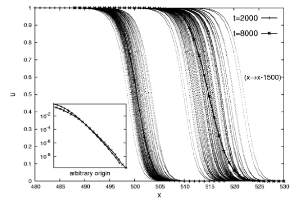
This is very well seen in a numerical simulation of reaction-diffusion models, see Fig. 31. There is an interesting consequence of this fact: The average of $u(x,t)$ over the noise does not depend on the geometric scaling variable $x-\langle X(t)\rangle$, but on a different variable:

$$\langle u(x,t)\rangle={\cal U}\left(\frac{x-\langle X(t)\rangle}{\sqrt{t/\ln^{3}N}}\right).$$ (168)

This is again seen in Fig. 31, see the inset. This new scaling which replaces geometric scaling at very large times is sometimes called “diffusive scaling”. We leave the proof as an exercise for the reader.

Exercise 9.

Prove the diffusive scaling pattern (168) for $u(x,t)$ averaged over the realizations. Remember that each realization of the stochastic evolution looks like a deterministic traveling wave with shape which may be approximated by

$$u(x,t)=\theta(x-X(t))e^{-\gamma_{0}x}+\theta(X(t)-x),$$ (169)

and that $X(t)$ is a stochastic variable whose distribution, for the purpose of this calculation, can be approximated by a Gaussian of width $\sim\sqrt{t/\ln^{3}N}$.

4.4 Applications to QCD: Beyond BK

We have argued that in the context of QCD, a nonlinear mechanism (something like gluon recombination?) should supplement the dipole model to tame the exponential growth of the dipole/gluon density with the rapidity as soon as the . The equations which would describe such effects are not yet known for sure.

We have just analyzed most generally reaction-diffusion models, which are very similar to the dipole model for the linear part (diffusion and exponential growth of the number of objects), supplemented with recombination which, on the average, effectively limits the density of particles to $N$. The results we obtained for the front position and for the shape of the particle density depend only on the branching-diffusion process (through the eigenvalues $\chi(\gamma)$) and in $N$.

So it is enough to use the dictionary (1) to which one adds the QCD quantity corresponding to $N$, namely $1/\alpha_{s}^{2}$, in order to be able to take over the results found above for the front position (167) and particle density profile (168) in reaction-diffusion processes to scattering amplitudes in QCD. We therefore arrive at predictions for the rapidity-dependence of the saturation scale, and we also predict a departure from geometric scaling at very high rapidities.

   Intermediate recap
We have argued that there should be some kind of nonlinearity which effectively limits the density of gluons (or equivalently of dipoles) in the quantum evolution to $\sim 1/\alpha_{s}^{2}$. The precise mechanism is not known in QCD, but one may get an idea of the effects of such nonlinearities in simple branching-diffusion models with recombination (reaction-diffusion, or population evolution). We found that realizations of such models are stochastic traveling waves. Their position is now a random variable. We were able to compute all its cumulants, which depend only on a few parameters and not on the details of the recombination mechanism: This universality enables one to take over the results obtained in generic reaction-diffusion models to QCD, although the proper evolution equation has not been derived in QCD. We found that the main physical consequence on the QCD amplitudes is the substitution of geometric scaling by diffusive scaling at ultrahigh rapidities. $\blacksquare$   

5 Conclusion

5.1 Summary: the big picture

Let us summarize the picture to which we have arrived in these lectures for the rapidity evolution of scattering amplitudes.

We were concerned essentially with dipole-nucleus scattering for which the BK equation seems firmly established, but in the last section, we turned also to dipole-dipole scattering.

We were able to identify three (well-)separated rapidity scales, which delimitate 4 regimes:

• Region I: Low-density region. The BFKL equation is valid since the gluon density is low. Of course, it applies both to dipole-dipole and dipole-nucleus scattering.

• Region II: High density. When the rapidity is higher than $y_{\text{sat}}$, nonlinear effects set in. In the dipole-nucleus case, for $y_{\text{sat}}\ll y_{\text{diff}}$, the latter correspond to independent multiple scatterings between the evolved dipole and the target. They are described by the BK equation. In the dipole-dipole case instead, the BK equation cannot be established since the nonlinear effects are to be included in the evolution itself. The right equation may be something like a “stochastic BK equation”. However, it seems that in this region, the scattering amplitude has the same properties as if it were a solution of the BK equation. In particular, it exhibits geometric scaling.

• Region III: Modified saturation scale. The BK equation breaks down at this point also in the diple-nucleus case. The saturation scale becomes independent of the rapidity. Geometric scaling still holds: More precisely, it seems that the scaling variable is the same, but the precise shape of the amplitude is different in the dipole-dipole and dipole nucleus cases, see the recent work of ours, Ref. [MM14a].

• Region IV: Diffusive scaling. One enters a regime dominated by fluctuations, which manifest themselves in the form of a new scaling form for the amplitude, “diffusive scaling”. This holds both for the dipole-dipole and the dipole-nucleus amplitudes.

5.2 Historical note

Our presentation of these topics may lead one to think that geometric scaling was predicted from the mathematics exposed here, and then found in the data. Actually, the story went almost exactly the other way round. Let us briefly sketch the main steps which led to the understanding of QCD amplitudes at very high energies that we have explained here. (Of course, we do not claim exhaustivity).

The Balitsky-Kovchegov equation was first established in 1996 [Bal96], and rederived in 1999 in the context of the dipole model [Kov99, Kov00]. Until year 2000, no one knew how to solve it. In the meantime, Golec-Biernat and Wüsthoff proposed a saturation model [GBW99, GBW98] which described very well virtually all HERA data in the small-$x$ regime. Geometric scaling was accidentally postulated in this model, a fact which was noticed by Staśto, Golec-Biernat and Kwieciński and subsequently discovered in the data [SGBK01]. Attemps to derive geometric scaling from QCD were made in the next few years, first through numerical works, and then analytically [GBMS02, IIM02, MT02]. (Actually, the form of the rapidity dependence of the saturation scale, namely what we related in these lectures to the velocity of the traveling wave $\bar{\alpha}_{s}\chi(\gamma_{0})/\gamma_{0}$, was known much before from the solution of the first equation for saturation derived from physical arguments by Gribov, Levin, Ryskin [GLR83]) (and in in the double-leading logarithmic approximation by Mueller and Qiu [MQ86]). The interpretation of geometric scaling as FKPP traveling waves came only after [MP03, MP04]. The first attempt to go beyond the BK equation was achieved in Ref. [MS04], and the result obtained there was then recognized to stem also from the stochastic FKPP equation and to be related to the discreteness of quanta in Ref. [IMM05].

5.3 Concluding remarks and prospects

We recognized that the BK equation, which governs the rapidity/energy evolution of QCD amplitudes in the high-energy limit, belongs to a large universality class, whose simplest representative is the FKPP equation.

Essentially, this holds because parton evolution is a peculiar branching diffusion process. This is likely to be a very general statement, beyond the particular realization of parton evolution (namely the color dipole model) we have been focusing on in these lectures.

This identification is useful because many of the main properties of traveling waves are universal: They can be understood on simple toy models, and the obtained results can then simply be taken over to QCD.

From the mathematical point of view, we are trying to understand the properties of solutions (or better, realizations) of nonlinear (stochastic) partial differential equations. Since the latter appear in many different fields, any progress in this direction may have numerous potential applications.

From the physical point of view, this link between QCD and more general mathematical problems can help to understand the very essence of saturation in QCD, and also to learn how to go beyond the BK equation. It sets a general framework for understanding saturation effects, which are conceptually interesting, and are likely to play an important role for the phenomenology at the LHC.

Appendix A Computation of the complex integral which appears in the BFKL eigenvalue problem

In this section, we shall compute the integral

$$I=\int\frac{dzd\bar{z}}{2i}z^{\alpha-1}\bar{z}^{\tilde{\alpha}-1}(1-z)^{\beta-1}(1-\bar{z})^{\tilde{\beta}-1}.$$ (170)

Such integrals appear in the context of various problems involving conformal field theory, and the computation below may be found in different places in the literature (see e.g. [DFMS97] for a textbook, or Ref. [Xia08] Appendix A, or [CM11] or Ref. [GN03] for a more general integral of this type).

For $I$ to be well defined, the integrand must have trivial monodromies around the singularities at $z=0,1$. This is the case if $\alpha-\tilde{\alpha}$, $\beta-\tilde{\beta}$ are integer numbers. We shall restrict ourselves to real exponents, which simplifies the discussion and is enough for the purposes of this paper. Furthermore, the integral converges only if $\text{Re}(\alpha+\tilde{\alpha})>0$, $\text{Re}(\beta+\tilde{\beta})>0$ (at $z=0,1$) and $\text{Re}(\alpha+\tilde{\alpha}+\beta+\tilde{\beta})<2$ (at $|z|\rightarrow\infty$).

Our calculation is a heuristic way to arrive at an expression for this integral in terms of known functions.

The first step is to write $I$ as a double integral over real variables. Defining $z\equiv x+iy$, one gets

$$I=\int_{-\infty}^{+\infty}dx\int_{-\infty}^{+\infty}dy(x+iy)^{\alpha-1}(x-iy)^{\tilde{\alpha}-1}(1-x-iy)^{\beta-1}(1-x+iy)^{\tilde{\beta}-1}.$$ (171)

Then, one performs a Wick rotation $y\rightarrow e^{i(\pi/2-2\varepsilon)}y\simeq i(1-2i\varepsilon)y$, where the term proportional to $\varepsilon$ hampers that the integration path go along the branch cuts. We get

$$I=i\int_{-\infty}^{+\infty}dx\int_{-\infty}^{+\infty}dy(x-y+2i\varepsilon y)^{\alpha-1}(x+y-2i\varepsilon y)^{\tilde{\alpha}-1}(1-x+y-2i\varepsilon y)^{\beta-1}\\ \times(1-x-y+2i\varepsilon y)^{\tilde{\beta}-1}.$$ (172)

Next, the change of variables $X_{+}=x+y$, $X_{-}=x-y$ casts the integral in the form

$$I=-\frac{i}{2}\int_{-\infty}^{+\infty}dX_{+}\int_{-\infty}^{+\infty}dX_{-}[X_{-}+i\varepsilon(X_{+}-X_{-})]^{\alpha-1}[X_{+}-i\varepsilon(X_{+}-X_{-})]^{\tilde{\alpha}-1}\\ \times[1-X_{-}-i\varepsilon(X_{+}-X_{-})]^{\beta-1}[1-X_{+}+i\varepsilon(X_{+}-X_{-})]^{\tilde{\beta}-1}.$$ (173)

The integration over $X_{+}$ may be written as a sum of contributions from the integration domains $]-\infty,0[$, $]0,1[$, $]1,+\infty[$. The position of the branch points in the $X_{-}$ plane with respect to the integration contour is then specified:

$$X_{-}=-i\varepsilon X_{+}\ ,\ \ X_{-}=1-i\varepsilon(X_{+}-1).$$ (174)

Note however that the $X_{-}$ contour crosses the cuts. For example for $X_{+}\in]-\infty,0[$, there is a cut along the negative real axis in the $X_{-}$ plane, which intersects the contour at $X_{-}=X_{+}$: The branch point at $0$ is in the upper-$X_{-}$ plane, but the cut then goes to the lower plane when $X_{-}<X_{+}$. But as we shall see, this is not a problem since the initial integral is well defined. Let us write the contribution of the integration region $(X_{+},X_{-})\in]-\infty,0[^{2}$ as

$$I_{11}=-\frac{i}{2}\int_{-\infty}^{0}dX_{+}\bigg{[}\int_{-\infty}^{X_{+}}dX_{-}(X_{-}+i\varepsilon)^{\alpha-1}(X_{+}-i\varepsilon)^{\tilde{\alpha}-1}f(X_{+},X_{-})\\ +\int_{X_{+}}^{0}dX_{-}(X_{-}-i\varepsilon)^{\alpha-1}(X_{+}+i\varepsilon)^{\tilde{\alpha}-1}f(X_{+},X_{-})\bigg{]},$$ (175)

where $f(X_{+},X_{-})$ gathers the remaining factors, which are real on the contours of integration considered here. Since

$$\int_{-\infty}^{0}dX_{+}\int_{-\infty}^{X_{+}}dX_{-}(X_{-}+i\varepsilon)^{\alpha-1}(X_{+}-i\varepsilon)^{\tilde{\alpha}-1}f(X_{+},X_{-})\\ =e^{-2i\pi(\alpha-\tilde{\alpha})}\int_{-\infty}^{0}dX_{+}\int_{-\infty}^{X_{+}}dX_{-}(X_{-}-i\varepsilon)^{\alpha-1}(X_{+}+i\varepsilon)^{\tilde{\alpha}-1}f(X_{+},X_{-}),$$ (176)

and since $\alpha-\tilde{\alpha}$ is an integer, the contributions of the discontinuity at $X_{+}=X_{-}$ cancel between the two integrations and the cut may safely be kept in the upper plane for all relevant values of $X_{+}$ and $X_{-}$. The same must be true also for the other cases.

The contours in the $X_{-}$ plane are shown in Fig. 32 in the different ranges of $X_{+}$.

$X_{+}<0$	$0<X_{+}<1$	$X_{+}>1$

Figure 32: Integration contours for the $X_{-}$ variable corresponding to the different possible values of the $X_{+}$ variable.

We see that only the integral over $X_{-}$ in the domain $X_{+}\in]0,1[$ contributes to $I$, since in the other cases, the contour in the $X_{-}$ plane may be shrunk to a point. After appropriate contour deformations, one gets

$$I=\sin\pi\alpha\int_{0}^{1}dX_{+}X_{+}^{\tilde{\alpha}-1}(1-X_{+})^{\tilde{\beta}-1}\times\int_{-\infty}^{0}dX_{-}(-X_{-})^{\alpha-1}(1-X_{-})^{\beta-1}$$ (177)

The sine factor comes from the discontinuity across the cut $]-\infty,0]$. The integral over $X_{+}$ clearly is the beta function $B(\tilde{\alpha},\tilde{\beta})$. Indeed, the latter is defined by

$$B(a,b)=\int_{0}^{1}dx\,x^{a-1}(1-x)^{b-1},$$ (178)

and admits a representation in terms of $\Gamma$ functions:

$$B(a,b)=\frac{\Gamma(a)\Gamma(b)}{\Gamma(a+b)}.$$ (179)

This relation may be proven as follows. Using the definitions of the $\Gamma$ function (Eq. (80)) and of the $B$ function (Eq. (179), we write

$$\Gamma(a+b)B(a,b)=\int_{0}^{\infty}dy\,y^{a+b-1}e^{-y}\int_{0}^{1}dx\,x^{a-1}(1-x)^{b-1},$$ (180)

and perform the change of variable $x=X/y$. Then

$$\Gamma(a+b)B(a,b)=\int_{0}^{\infty}dy\,e^{-y}\int_{0}^{y}dX\,X^{a-1}(y-X)^{b-1}.$$ (181)

Next, we exchange the order of the integrations and subsequently shift the $y$-variable by $X$:

$$\int_{0}^{\infty}dy\,e^{-y}\int_{0}^{y}dX\,X^{a-1}(y-X)^{b-1}=\int_{0}^{\infty}dX\,X^{a-1}\int_{X}^{\infty}dy\,(y-X)^{b-1}e^{-y}\\ =\int_{0}^{\infty}dX\,X^{a-1}e^{-X}\int_{0}^{\infty}dy\,y^{b-1}e^{-y},$$ (182)

which is simply the product $\Gamma(a)\Gamma(b)$.

The integral over $X_{-}$ in Eq. (177) reduces to $B({\alpha,1-\alpha-\beta})$ after the change of variable $X_{-}=x/(x-1)$ has been performed. Using the identity

$$\frac{\pi}{\sin\pi x}=\Gamma(x)\Gamma(1-x),$$ (183)

one may rewrite $I$ in several equivalent ways. Useful formulas are

$$I=\pi\frac{\Gamma(\tilde{\alpha})\Gamma(\tilde{\beta})}{\Gamma(\tilde{\alpha}+\tilde{\beta})}\frac{\Gamma(1-\alpha-\beta)}{\Gamma(1-\alpha)\Gamma(1-\beta)}=B({\alpha,\beta})B({\tilde{\alpha},\tilde{\beta}})\frac{\sin\pi\alpha\sin\pi\beta}{\sin\pi(\alpha+\beta)}.$$ (184)

References

- [Bal96] I. Balitsky. Operator expansion for high-energy scattering. Nucl.Phys., B463:99–160, 1996.
- [BD97] Eric Brunet and Bernard Derrida. Shift in the velocity of a front due to a cutoff. Phys. Rev. E, 56:2597–2604, Sep 1997.
- [BDMM06a] E. Brunet, B. Derrida, A.H. Mueller, and S. Munier. A Phenomenological theory giving the full statistics of the position of fluctuating pulled fronts. Phys.Rev., E73:056126, 2006.
- [BDMM06b] E. Brunet, B. Derrida, A.H. Mueller, and S. Munier. Noisy traveling waves: Effect of selection on genealogies. Europhys.Lett., 76:1–7, 2006.
- [CLM14] Carlos Contreras, Eugene Levin, and Rodrigo Meneses. Non linear evolution: revisiting the solution in the saturation region. 2014.
- [CM11] M. Ciafaloni and S. Munier. Hamiltonian solutions of the 3-body problem in (2+1)-gravity. Class.Quant.Grav., 28:195018, 2011.
- [DFMS97] P. Di Francesco, P. Mathieu, and D. Senechal. Conformal field theory. 1997.
- [EGBM05] R. Enberg, Krzysztof J. Golec-Biernat, and S. Munier. The High energy asymptotics of scattering processes in QCD. Phys.Rev., D72:074021, 2005.
- [EvS00] Ute Ebert and Wim van Saarloos. Front propagation into unstable states: universal algebraic convergence towards uniformly translating pulled fronts. Physica D: Nonlinear Phenomena, 146(1–4):1 – 99, 2000.
- [FILM02] Elena Ferreiro, Edmond Iancu, Andrei Leonidov, and Larry McLerran. Nonlinear gluon evolution in the color glass condensate. 2. Nucl.Phys., A703:489–538, 2002.
- [Gar04] C. W. Gardiner. Handbook of stochastic methods for physics, chemistry and the natural sciences, volume 13 of Springer Series in Synergetics. Springer-Verlag, third edition, 2004.
- [GBMS02] Krzysztof J. Golec-Biernat, L. Motyka, and A.M. Stasto. Diffusion into infrared and unitarization of the BFKL pomeron. Phys.Rev., D65:074037, 2002.
- [GBW98] Krzysztof J. Golec-Biernat and M. Wusthoff. Saturation effects in deep inelastic scattering at low and its implications on diffraction. Phys.Rev., D59:014017, 1998.
- [GBW99] Krzysztof J. Golec-Biernat and M. Wusthoff. Saturation in diffractive deep inelastic scattering. Phys.Rev., D60:114023, 1999.
- [GLR83] L.V. Gribov, E.M. Levin, and M.G. Ryskin. Semihard Processes in QCD. Phys.Rept., 100:1–150, 1983.
- [GN03] Jeffrey S. Geronimo and Henri Navelet. On certain integrals that appear in conformal field theory. J.Math.Phys., 44(5):2293–2319, May 2003.
- [IIM02] Edmond Iancu, Kazunori Itakura, and Larry McLerran. Geometric scaling above the saturation scale. Nucl.Phys., A708:327–352, 2002.
- [IIM04] E. Iancu, K. Itakura, and S. Munier. Saturation and BFKL dynamics in the HERA data at small x. Phys.Lett., B590:199–208, 2004.
- [ILM01] Edmond Iancu, Andrei Leonidov, and Larry D. McLerran. Nonlinear gluon evolution in the color glass condensate. 1. Nucl.Phys., A692:583–645, 2001.
- [IMM05] E. Iancu, A.H. Mueller, and S. Munier. Universal behavior of QCD amplitudes at high energy from general tools of statistical physics. Phys.Lett., B606:342–350, 2005.
- [KL12] Y.V. Kovchegov and E. Levin. Quantum Chromodynamics at High Energy. Cambridge Monographs on Particle Physics, Nuclear Physics and Cosmology. Cambridge University Press, 2012.
- [Kov99] Yuri V. Kovchegov. Small x F(2) structure function of a nucleus including multiple pomeron exchanges. Phys.Rev., D60:034008, 1999.
- [Kov00] Yuri V. Kovchegov. Unitarization of the BFKL pomeron on a nucleus. Phys.Rev., D61:074018, 2000.
- [LK14] Agnieszka Luszczak and Henri Kowalski. Dipole model analysis of high precision HERA data. Phys.Rev., D89:074051, 2014.
- [LT00] E. Levin and K. Tuchin. Solution to the evolution equation for high parton density QCD. Nucl.Phys., B573:833–852, 2000.
- [MM14a] A.H. Mueller and S. Munier. On parton number fluctuations at various stages of the rapidity evolution. Phys.Lett., B737:303–310, 2014.
- [MM14b] A.H. Mueller and S. Munier. Phenomenological picture of fluctuations in branching random walks. 2014.
- [MP03] S. Munier and Robert B. Peschanski. Geometric scaling as traveling waves. Phys.Rev.Lett., 91:232001, 2003.
- [MP04] S. Munier and Robert B. Peschanski. Traveling wave fronts and the transition to saturation. Phys.Rev., D69:034008, 2004.
- [MQ86] Alfred H. Mueller and Jian-wei Qiu. Gluon Recombination and Shadowing at Small Values of x. Nucl.Phys., B268:427, 1986.
- [MS04] A.H. Mueller and A.I. Shoshi. Small- physics beyond the Kovchegov equation. Nucl.Phys., B692:175–208, 2004.
- [MS06] C. Marquet and L. Schoeffel. Geometric scaling in diffractive deep inelastic scattering. Phys.Lett., B639:471–477, 2006.
- [MT02] A.H. Mueller and D.N. Triantafyllopoulos. The Energy dependence of the saturation momentum. Nucl.Phys., B640:331–350, 2002.
- [Mue94] Alfred H. Mueller. Soft gluons in the infinite momentum wave function and the BFKL pomeron. Nucl.Phys., B415:373–385, 1994.
- [Mun09] S. Munier. Quantum chromodynamics at high energy and statistical physics. Phys.Rept., 473:1–49, 2009.
- [MV94a] Larry D. McLerran and Raju Venugopalan. Computing quark and gluon distribution functions for very large nuclei. Phys.Rev., D49:2233–2241, 1994.
- [MV94b] Larry D. McLerran and Raju Venugopalan. Gluon distribution functions for very large nuclei at small transverse momentum. Phys.Rev., D49:3352–3355, 1994.
- [Pel85] Peliti, L. Path integral approach to birth-death processes on a lattice. J. Phys. France, 46(9):1469–1483, 1985.
- [RW04] Kari Rummukainen and Heribert Weigert. Universal features of JIMWLK and BK evolution at small x. Nucl.Phys., A739:183–226, 2004.
- [SGBK01] A.M. Staśto, Krzysztof J. Golec-Biernat, and J. Kwieciński. Geometric scaling for the total cross-section in the low- region. Phys.Rev.Lett., 86:596–599, 2001.
- [vS03] Wim van Saarloos. Front propagation into unstable states. Physics Reports, 386(2–6):29 – 222, 2003.
- [Xia08] Bo-Wen Xiao. On the anomalous dimensions of the multiple pomeron exchanges. Nucl.Phys., A798:132–164, 2008.