Active space decomposition with multiple sites: Density matrix renormalization group algorithm

Abstract

We extend the active space decomposition method, recently developed by us, to more than two active sites using the density matrix renormalization group algorithm. The fragment wave functions are described by complete or restricted active-space wave functions. Numerical results are shown on a benzene pentamer and a perylene diimide trimer. It is found that the truncation errors in our method decrease almost exponentially with respect to the number of renormalization states $M$, allowing for numerically exact calculations (to a few $\mu E_{\mathrm{h}}$ or less) with $M=128$ in both cases. This rapid convergence is because the renormalization steps are used only for the interfragment electron correlation.

The electronic structure of organic aggregates and crystals has been studied to characterize and predict electron and exciton dynamics in organic photovoltaics and light emitting devices.Coropceanu et al. (2007) While the majority of computational studies of such processes has been performed using density functional theory (DFT), processes that involve multiple excitons, such as singlet fission,Smith and Michl (2010) cannot be well described by standard time-dependent DFT, which has stimulated the development of accurate wave function theories for these systems.

We have recently developed a method, called active-space decomposition (ASD),Parker et al. (2013) which alleviates the large computational cost of active-space methods by tailoring the wave function ansatz to molecular dimers. In ASD, a dimer wave function $\Psi$ is compactly expressed as a linear combination of tensor products of monomer wave functions, i.e.,

$$|\Psi\rangle=\sum_{IJ}C_{IJ}|\Phi^{A}_{I}\rangle\otimes|\Phi^{B}_{J}\rangle\equiv\sum_{IJ}C_{IJ}|\Phi^{A}_{I}\Phi^{B}_{J}\rangle,$$ (1)

where $A$ and $B$ label monomers, and $I$ and $J$ label orthonormal monomer states. This expression is exact when the complete set of states is included in the sum; practically the number of states in the summation is set to a finite value. We have shownParker et al. (2013) that by choosing monomer wave functions that diagonalize a monomer Hamiltonian within the orthogonal subspace (i.e., $\hat{H}^{A}|\Phi^{A}_{I}\rangle=E^{A}_{I}|\Phi^{A}_{I}\rangle$), dimer wave functions rapidly converge to the exact solution with respect to the number and type of monomer states. This product basis is also related to quasi-diabatic representation of the model space.Parker and Shiozaki (2014) ASD is compatible with any wave function method for which transition density matrices are available. In particular, efficient implementation of ASD has been realized with complete active space (CAS) and restricted active spaceOlsen et al. (1988) (RAS) monomer wave functions. ASD has been used to compute model Hamiltonians for dynamical processes such as singlet fission in tetracene and pentacene dimersParker et al. (2014) and charge and triplet energy transfer in benzene dimers.Parker and Shiozaki (2014)

Here, we extend ASD beyond dimers to incorporate an arbitrary number of fragments:

$$|\Psi\rangle=\sum_{IJK\cdots}C_{IJK\cdots}|\Phi^{A}_{I}\rangle\otimes|\Phi^{B}_{J}\rangle\otimes|\Phi^{C}_{K}\rangle\otimes\cdots,$$ (2)

where $I$, $J$, and $K$ formally run over the complete set of states on each fragment. The coefficient tensor $C_{IJK\cdots}$ is approximated by matrix product states used in the density matrix renormalization group (DMRG) algorithm,

$$C_{IJK\cdots}=\mathrm{Tr}[\mathbf{C}^{A,I}\mathbf{C}^{B,J}\mathbf{C}^{C,K}\cdots],$$ (3)

in which the dimension of matrices $\mathbf{C}$ is set to a predetermined value $M$. First described by White and used to compute ground and excited states of the Heisenberg spin chain,White (1992, 1993) DMRG has proven to be a powerful tool that provides numerically exact solutions with polynomial cost even for strongly correlated systems.White and Martin (1999); Zgid and Chan (2009); Kurashige and Yanai (2009); Marti and Reiher (2010); Chan and Sharma (2011); Wouters and Van Neck (2014) In chemical applications, DMRG has enabled highly accurate calculations on strongly correlated electronic structure of molecules or complexes that are intractable with traditional active-space methods.Kurashige, Chan, and Yanai (2013); Sharma et al. (2014)

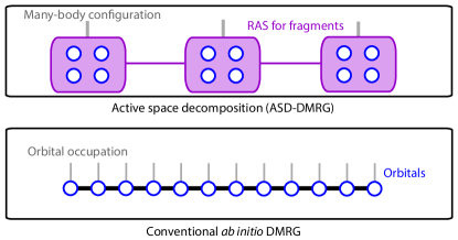
Figure 1: Comparison of wave functions in ASD-DMRG and in conventional ab initio DMRG.

We start by sketching the ASD-DMRG algorithm, which is formulated in terms of a one-dimensional chain of $n$ sites (see Fig. 1). In the conventional ab initio DMRG, these sites are chosen to be one-electron orbitals.White and Martin (1999) In this work, we choose each site to be the CAS or RAS wave function of a single molecule or fragment, alleviating the orbital ordering problem in the conventional ab initio DMRG algorithmMoritz, Hess, and Reiher (2005); Rissler, Roack, and White (2006) and allowing for applications to three-dimensional structures. As a consequence, the dimensionality of the single site, $d$, is much larger in ASD-DMRG than in conventional approaches. However, a key result of this study is that this allows $M$ to be very small. Since calculations involving the full configurational space of a molecular dimer are intractable for large molecules of materials interest, we have implemented the single-site variant of the DMRG algorithm.White (2005) The single-site algorithm converges more smoothly than the two-site algorithm, though it is more prone to getting stuck in local minima during the optimization (see below).White (2005); Zgid and Nooijen (2008a)

The chain is initiated by computing a user-defined number of low-lying eigenstates of the first site. We will represent the $i$-th single site as $\bullet_{i}$. These states are then renormalized to form a block, i.e. $L_{1}\leftarrow\bullet_{1}$ with $L_{i}$ referring to a block containing $i$ sites. Next, a new site is added to the chain to form $L_{1}\bullet_{2}$, and several low-lying eigenstates of this block-site system are computed and renormalized as $L_{2}\leftarrow L_{1}\bullet_{2}$. This process is continued until each site has been added to the chain. During this growing phase, the sites that have yet to be incorporated into the block are included at the mean-field level. This is equivalent to using a tensor product of the Hartree–Fock ground state of each site as the initial guess. Such a mean-field initial guess is well-defined in the case where each site is a distinct molecule, although other initial guesses may be necessary in the case where sites are covalently bound.

The final stage of the algorithm involves “sweeping” along the chain to optimize the renormalized states. In each step of the sweep, a system $L_{i-1}\bullet_{i}R_{n-i}$ is diagonalized, which contains a left block describing $i-1$ sites $L_{i-1}$, a right block describing $n-i$ sites $R_{n-i}$, and the $i$-th single site, $\bullet_{i}$. The wave function at this step is written as

$$|\Psi\rangle =\sum^{M}_{\mu\nu}\sum_{\phi}C^{i,\phi}_{\mu\nu}|\Phi^{L_{i-1}}_{\mu}\rangle\otimes|\phi^{i}\rangle\otimes|\Phi^{R_{n-i}}_{\nu}\rangle$$

$$=\sum^{M}_{\mu\nu}|\Phi^{L_{i-1}}_{\mu}\Phi^{i}_{\mu\nu}\Phi^{R_{n-i}}_{\nu}\rangle,$$ (4)

where $|\phi^{i}\rangle$ is a Slater determinant only with orbitals on the site $i$, $|\Phi^{L_{i-1}}_{\mu}\rangle$ is a renormalized left-block state, $|\Phi^{R_{n-i}}_{\nu}\rangle$ is a renormalized right-block state, and $|\Phi^{i}_{\mu\nu}\rangle\equiv\sum_{\phi}C^{i,\phi}_{\mu\nu}|\phi\rangle$. The key insight behind the DMRG algorithm is that the optimal block states to represent the combined $L_{i-1}\bullet_{i}$ part of the chain can be obtained by the Schmidt decomposition of the reduced density matrix (RDM),

$$\hat{\rho}_{L_{i-1}\bullet_{i}}=\text{Tr}\left[|\Psi\rangle\langle\Psi|\right]_{R_{n-i}},$$ (5)

where the trace is over all states in the right block. Thus, one computes and diagonalizes the RDM in each step of the sweep and uses the $M$ eigenvectors corresponding to the largest eigenvalues to renormalize $L_{i}\leftarrow L_{i-1}\bullet_{i}$.

To diagonalize the Hamiltonian during the sweep, we resolve the Hamiltonian in terms of the renormalized block states $\{\Phi^{L}_{\mu}\}$ and $\{\Phi^{R}_{\nu}\}$. Defining $|\Phi^{B}_{\mu\nu}\rangle\equiv|\Phi^{L}_{\mu}\rangle\otimes|\Phi^{R}_{\nu}\rangle$ and following the notation of Kurashige and Yanai,Kurashige and Yanai (2009) we write the Hamiltonian as

$$\hat{H}= \hat{H}^{B}+\hat{H}^{i}+\sum_{p_{B}}\left(\hat{T}^{i}_{p_{B}}\hat{p}_{B}+\hat{p}_{B}^{\dagger}\hat{T}^{i\dagger}_{p_{B}}\right)$$

$$+ \sum_{p_{i}}\left(\hat{S}^{B}_{p_{i}}\hat{p}_{i}+\hat{p}_{i}^{\dagger}\hat{S}^{B\dagger}_{p_{i}}\right)+\sum_{p_{i}q_{i}}\hat{p}_{i}^{\dagger}\hat{q}_{i}\hat{Q}^{B}_{p_{i}q_{i}}$$

$$+ \sum_{p_{i}r_{i}}\left(\hat{p}_{i}^{\dagger}\hat{r}_{i}^{\dagger}\hat{P}^{B}_{p_{i}r_{i}}+\hat{P}^{B\dagger}_{p_{i}r_{i}}\hat{p}_{i}\hat{r}_{i}\right),$$ (6)

in which we have introduced the following operators:

$$\hat{H}^{X}= \sum_{p_{X}q_{X}}\hat{p}_{X}^{\dagger}\hat{q}_{X}h_{p_{X}q_{X}}+\frac{1}{2}\sum_{p_{X}q_{X}r_{X}s_{X}}\hat{p}_{X}^{\dagger}\hat{q}_{X}^{\dagger}\hat{r}_{X}\hat{s}_{X}(p_{X}s_{X}|q_{X}r_{X}),$$ (7)

$$\hat{T}^{i}_{p_{B}}= \sum_{q_{i}r_{i}s_{i}}\hat{s}_{i}^{\dagger}\hat{r}_{i}^{\dagger}\hat{q}_{i}(p_{B}s_{i}|q_{i}r_{i}),$$ (8)

$$\hat{S}^{B}_{p_{i}}= \sum_{q_{B}}\hat{q}_{B}^{\dagger}h_{p_{i}q_{B}}+\sum_{q_{B},r_{B},s_{B}}\hat{s}_{B}^{\dagger}\hat{r}_{B}^{\dagger}\hat{q}_{B}(p_{i}s_{B}|q_{B}r_{X}),$$ (9)

$$\hat{P}^{B}_{p_{i}r_{i}}= \sum_{q_{i}s_{i}}\hat{q}_{i}\hat{s}_{i}(p_{B}s_{i}|q_{i}r_{B}),$$ (10)

$$\hat{Q}^{B}_{p_{i}q_{i}}= \sum_{r_{i}s_{i}}\hat{r}_{i}^{\dagger}\hat{s}_{i}\left[(p_{B}q_{B}|r_{i}s_{i})-(p_{B}r_{i}|q_{B}s_{i})\right].$$ (11)

Here $X$ is either $B$ or $i$, $\hat{p}_{X}$ ($\hat{p}_{X}^{\dagger})$ is the annihilation (creation) operator for orbital $p$ on site/block $X$, $h_{pq}$ is a matrix element of the one-electron operator and $(pq|rs)$ is a matrix element of the two-electron Coulomb operator. In our algorithm, we compute and store transition density matrices whose indices belong to the same block using an algorithm developed in Refs. Parker et al., 2013; Parker and Shiozaki, 2014. For instance,

$$\Gamma^{Z,\lambda^{\prime}\lambda}_{p^{\dagger}q}\equiv\langle\Phi^{Z}_{\lambda^{\prime}}|\hat{p}^{\dagger}\hat{q}|\Phi^{Z}_{\lambda}\rangle,$$ (12)

where $Z$ is either $L$ or $R$, $\lambda$ is either $\mu$ or $\nu$, and $\Gamma^{Z,\lambda^{\prime}\lambda}_{p^{\dagger}q^{\dagger}r}$, $\Gamma^{Z,\lambda^{\prime}\lambda}_{pq}$, and $\Gamma^{Z,\lambda^{\prime}\lambda}_{p}$ are likewise defined. The block operators of Eq. (Active space decomposition with multiple sites: Density matrix renormalization group algorithm) are resolved using these transition densities, e.g.,

$$\langle\Phi^{B}_{\mu^{\prime}\nu^{\prime}}|\hat{P}^{B}_{p_{i}r_{i}} |\Phi^{B}_{\mu\nu}\rangle=\delta_{\nu^{\prime}\nu}\sum_{q_{L}s_{L}}\Gamma^{L,\mu^{\prime}\mu}_{q_{L}s_{L}}(p_{i}s_{L}|r_{i}q_{L})$$

$$+ \delta_{\mu^{\prime}\mu}\sum_{q_{R}s_{R}}\Gamma^{R,\nu^{\prime}\nu}_{q_{R}s_{R}}(p_{i}s_{R}|r_{i}q_{R})$$

$$- (-1)^{N_{L_{\mu}}}\sum_{q_{R}}\Gamma^{R,\nu^{\prime}\nu}_{q_{R}}\sum_{s_{L}}\Gamma^{L,\mu^{\prime}\mu}_{s_{L}}(p_{i}s_{L}|r_{i}q_{R})$$

$$+ (-1)^{N_{L_{\mu}}}\sum_{q_{L}}\Gamma^{L,\mu^{\prime}\mu}_{q_{L}}\sum_{s_{R}}\Gamma^{R,\nu^{\prime}\nu}_{s_{R}}(p_{i}s_{R}|r_{i}q_{L}),$$ (13)

where $N_{L_{\mu}}$ is the number of electrons in $L_{\mu}$.

Active orbitals are identified as follows. We start by picking orbitals from monomer Hartree–Fock calculations using minimal basis. Then we perform Hartree–Fock on the full system and localize the canonical molecular orbitals to fragments using the Pipek–Mezey algorithm.Pipek and Mezey (1989) Finally, overlaps between these fragment-localized orbitals and the minimal-basis orbitals are used to automatically select active orbitals on each site.

Table 1: Total energies computed using $M=128$ and energy differences obtained with selected smaller values of $M$ for stacks of $n$ benzene molecules (in $E_{\mathrm{h}}$).

		$\Delta E$					$E_{\text{tot}}$
$n$	Active space	$M=1$	$M=4$	$M=8$	$M=16$	$M=32$	$M=128$
2	CAS(12,12)	$0.000501$	$0.000168$	$0.000134$	$0.000069$	$<0.000001$	$-461.179327$
3	CAS(18,18)	$0.001018$	$0.000343$	$0.000274$	$0.000141$	$0.000001$	$-691.768264$
4	CAS(24,24)	$0.001537$	$0.000520$	$0.000415$	$0.000214$	$0.000002$	$-922.357173$
5	CAS(30,30)	$0.002055$	$0.000696$	$0.000557$	$0.000287$	$0.000002$	$-1152.946072$

As is commonly known,White (2005); Zgid and Nooijen (2008a) the one-site DMRG algorithm is susceptible to getting stuck in local minima of the parameter space due to the fact that the algorithm does not spontaneously expand the range of quantum numbers in each site or block. For example, if a poor initial guess for the chain includes only neutral fragments and the total charge is constrained to be neutral, then the algorithm will keep only neutral fragment states although charge transfer configurations may be important in the exact ground state. To remedy this problem, we use the perturbative correction of WhiteWhite (2005) to the RDM [Eq. (5)], in which the RDM is supplemented by

$$\hat{\rho}_{L_{i-1}\bullet_{i}}^{\prime}=\hat{\rho}_{L_{i-1}\bullet_{i}}+a\sum_{\tau}\hat{O}^{i}_{\tau}\hat{\rho}_{L_{i-1}\bullet_{i}}\hat{O}^{i\dagger}_{\tau},$$ (14)

where $a>0$ is an arbitrary constant, and $\hat{O}^{i}_{\tau}$ is a site Hamiltonian operator (we use $\hat{p}_{i}$, $\hat{p}_{i}^{\dagger}$ and $\hat{p}_{i}^{\dagger}\hat{q}_{i}$). The constant $a$ is used to control the strength of the perturbation during the sweep. We typically start with a value of $10^{-3}$ and decrease it by one order of magnitude when the energy from successive sweeps changes by less than $10^{-7}$ $E_{\mathrm{h}}$. When $a$ reaches a minimum value ($a<10^{-7}$ in our calculations) the perturbation is turned off. With this scheme, we have seen that the final converged energies have no dependence on the initial guess.

Next, we show the numerical results on the ground state of a benzene stack consisting of 2 to 5 molecules with the def2-SVP basis set.Weigend and Ahlrichs (2005) The molecules are arranged cofacially with a separation of 4.0 Å (see Fig. 2a). The geometry of each benzene molecule was obtained in $D_{6{\text{h}}}$ symmetry using DFT with B3LYP functionalBecke (1993); Lee, Yang, and Parr (1988) and the def2-TZVPP basis set.Weigend and Ahlrichs (2005) Geometry optimization was performed using turbomole.Furche et al. (2014) Each benzene molecule is a single site containing six $\pi$ orbitals and six electrons. Using CAS wave functions on each site, the full stack is the equivalent of CAS(6$n$,6$n$). Calculations on a benzene dimer [for which the configuration interaction in CAS(12,12) is tractable] and those on a benzene trimer with a smaller active spacesup indicate that ASD-DMRG with $M=128$ recovered the CAS configuration interaction to within $10^{-7}$ $E_{\mathrm{h}}$. Thus, we consider $M=128$ to be fully converged for all benzene stack calculations. In Table 1, the total energies are compared to those obtained using smaller values of $M$. It is worth noting that the errors decrease almost exponentially with respect to $M$, and with as small as $M=32$, numerically exact results were obtained. The pentamer calculation with $M=128$ required about 2200 seconds per sweep on 128 CPU cores (9 sweeps) whereas the corresponding CAS(30,30) calculation, with $2.4\times 10^{16}$ total configurations, is intractable even for today’s most powerful supercomputers.

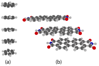
Figure 2: Geometries of the (a) benzene and (b) PDI stacks used in this work.

One of the advantages of ASD-DMRG over conventional DMRG is that occupation restrictions can be introduced on individual sites. To show this, we computed the ground state of the perylene diimide (PDI) dimer and trimer using RAS wave functions for each molecule (def2-SVP). PDI crystallizes into a slip-stacked configuration as shown in Fig. 2b.Guillermet et al. (2006) For monomers, we used geometries optimized using DFT under $D_{2\text{h}}$ symmetry with the def2-TZVPP basis setWeigend and Ahlrichs (2005) and the B3LYP density functional.Becke (1993); Lee, Yang, and Parr (1988) The dimer and trimer geometries were generated by adding a constant offset to the base unit of $(-3.34,1.11,3.38)$ Å where $x$ is the long axis of the molecule, $y$ is the short axis of the molecule, and $z$ is normal to the plane of the molecule. For single-site wave functions, we use RAS with 7 orbitals in RAS I, 4 orbitals in RAS III, and 7 orbitals in RAS II and a maximum of one hole in RAS I and one particle in RAS III. The tensor product of multiple RAS wave functions corresponds to a more general set of occupation restrictions than RAS itself: Each site can have one hole (particle) in RAS I (RAS III) rather than there being one hole (particle) allowed for the whole stack. The dimensionality of the product wave functions for the dimer and trimer is about $1\times 10^{7}$ and $2\times 10^{12}$, respectively.

The total energies computed for the PDI dimer and trimer are shown in Table 2. For the PDI dimer, we used up to $M=128$. As in the benzene case, the convergence of the total energy with respect to $M$ appears to be exponential. On the basis of these calculations we chose $M=48$ to compute the ground state of the PDI trimer. The energy difference between $M=128$ and $M=48$ for the dimer is about 0.06 $\mathrm{m}E_{\mathrm{h}}$. Noting that error in the total energy of the benzene stacks for a fixed $M$ was roughly proportional to $n-1$, we expect the total energy for the PDI trimer at $M=48$ to be accurate to within 0.2 $\mathrm{m}E_{\mathrm{h}}$. The trimer calculation with $M=48$ required ca. 1500 seconds per sweep using 256 CPU cores, although our program can be further optimized.

Table 2: Total energies (in $E_{\mathrm{h}}$) obtained for the PDI dimer and trimer at selected values of $M$.

$M$	dimer	trimer
1	$-2644.328613$	$-3966.487183$
4	$-2644.331085$	$-3966.492073$
8	$-2644.331681$	$-3966.493276$
16	$-2644.331990$	$-3966.493900$
32	$-2644.332199$	$-3966.494332$
48	$-2644.332283$	$-3966.494512$
72	$-2644.332327$	—
96	$-2644.332339$	—
128	$-2644.332343$	—

In conclusion, we have generalized the ASD method to incorporate multiple fragments (i.e., active sites). In this work the electronic structure of each fragment has been described by CAS and RAS wave functions. Our method is based on the matrix-product approximation of the coefficients [Eq. (3)], in which the wave functions are optimized using a density matrix renormalization group algorithm. We have shown that results with chemical accuracy (i.e., 1 $\mathrm{m}E_{\mathrm{h}}$ for total energies) can be obtained with a fairly small number of renormalization states $M$. This rapid convergence of the ASD-DMRG energy with respect to $M$ is the result of breaking the system into physically motivated fragments such that the renormalization steps are used to describe the interchromophore electron correlation, and not the intrachromophore correlation. Spin adaptationZgid and Nooijen (2008b); Sharma and Chan (2012) has not been done in this work. Application of ASD-DMRG to covalently bonded systems and investigation of the effects of site ordering will be studied in the future. All the programs reported in this work have been implemented in the open-source bagel package.bag

This work has been supported by Office of Basic Energy Sciences, U.S. Department of Energy (Grant No. DE-FG02-13ER16398).

References

- Coropceanu et al. (2007) V. Coropceanu, J. Cornil, D. A. da Silva Filho, Y. Olivier, R. Silbey, and J.-L. Brédas, Chem. Rev. 107, 926 (2007).
- Smith and Michl (2010) M. B. Smith and J. Michl, Chem. Rev. 110, 6891 (2010).
- Parker et al. (2013) S. M. Parker, T. Seideman, M. A. Ratner, and T. Shiozaki, J. Chem. Phys. 139, 021108 (2013).
- Parker and Shiozaki (2014) S. M. Parker and T. Shiozaki, J. Chem. Theory Comput. 10, 3738 (2014).
- Olsen et al. (1988) J. Olsen, B. O. Roos, P. Jørgensen, and H. J. Aa. Jensen, J. Chem. Phys. 89, 2185 (1988).
- Parker et al. (2014) S. M. Parker, T. Seideman, M. A. Ratner, and T. Shiozaki, J. Phys. Chem. C 118, 12700 (2014).
- White (1992) S. R. White, Phys. Rev. Lett. 69, 2863 (1992).
- White (1993) S. R. White, Phys. Rev. B 48, 10345 (1993).
- White and Martin (1999) S. R. White and R. L. Martin, J. Chem. Phys. 110, 4127 (1999).
- Zgid and Chan (2009) D. Zgid and G. K.-L. Chan, Annu. Rep. Comput. Chem. 5, 149 (2009).
- Kurashige and Yanai (2009) Y. Kurashige and T. Yanai, J. Chem. Phys. 130, 234114 (2009).
- Marti and Reiher (2010) K. H. Marti and M. Reiher, Z. Phys. Chem. 224, 583 (2010).
- Chan and Sharma (2011) G. K.-L. Chan and S. Sharma, Annu. Rev. Phys. Chem. 62, 465 (2011).
- Wouters and Van Neck (2014) S. Wouters and D. Van Neck, Eur. Phys. J. D 68, 272 (2014).
- Kurashige, Chan, and Yanai (2013) Y. Kurashige, G. K.-L. Chan, and T. Yanai, Nature Chem. 5, 660 (2013).
- Sharma et al. (2014) S. Sharma, K. Sivalingam, F. Neese, and G. K.-L. Chan, Nature Chem. 6, 927 (2014).
- Moritz, Hess, and Reiher (2005) G. Moritz, B. A. Hess, and M. Reiher, J. Chem. Phys. 122, 024107 (2005).
- Rissler, Roack, and White (2006) J. Rissler, R. M. Roack, and S. R. White, Chem. Phys. 323, 519 (2006).
- White (2005) S. R. White, Phys. Rev. B 72, 180403 (2005).
- Zgid and Nooijen (2008a) D. Zgid and M. Nooijen, J. Chem. Phys. 128, 144116 (2008a).
- Pipek and Mezey (1989) J. Pipek and P. G. Mezey, J. Chem. Phys. 90, 4916 (1989).
- Weigend and Ahlrichs (2005) F. Weigend and R. Ahlrichs, Phys. Chem. Chem. Phys. 7, 3297 (2005).
- Becke (1993) A. D. Becke, J. Chem. Phys. 98, 5648 (1993).
- Lee, Yang, and Parr (1988) C. Lee, W. Yang, and R. Parr, Phys. Rev. B 37, 785 (1988).
- Furche et al. (2014) F. Furche, R. Ahlrichs, C. Hättig, W. Klopper, M. Sierka, and F. Weigend, WIREs Comput. Mol. Sci. 4, 91 (2014).
- (26) See Supplementary Material Document No.xxxx for numerical tests of our implementation on the benzene dimer and trimer using a CAS(4,4) active space.
- Guillermet et al. (2006) O. Guillermet, M. Mossoyan-Déneux, M. Giorgi, A. Glachant, and J. C. Mossoyan, Thin Solid Films 514, 25 (2006).
- Zgid and Nooijen (2008b) D. Zgid and M. Nooijen, J. Chem. Phys. 128, 014107 (2008b).
- Sharma and Chan (2012) S. Sharma and G. K.-L. Chan, J. Chem. Phys. 136, 144105 (2012).
- (30) bagel, Brilliantly Advanced General Electronic-structure Library. http://www.nubakery.org under the GNU General Public License.