Dynamic adaptive multiple tests with finite sample FDR control

Abstract

The present paper introduces new adaptive multiple tests which rely on the estimation of the number of true null hypotheses and which control the false discovery rate (FDR) at level $\alpha$ for finite sample size. We derive exact formulas for the FDR for a large class of adaptive multiple tests which apply to a new class of testing procedures. In the following, generalized Storey estimators and weighted versions are introduced and it turns out that the corresponding adaptive step up and step down tests control the FDR. The present results also include particular dynamic adaptive step wise tests which use a data dependent weighting of the new generalized Storey estimators. In addition, a converse of the Benjamini and Hochberg (1995) theorem is given. The Benjamini and Hochberg (1995) test is the only “distribution free” step up test with FDR independent of the distribution of the $p$-values of false null hypotheses.

1 Introduction

Due to the multiplicity in multiple hypothesis testing, the control of a type I error rate is a serious problem. The familywise error rate (FWER) which is the probability of at least one false rejection is known to have a lack of power when the number of null hypotheses $n$ is large. Therefore, Benjamini and Hochberg (1995) promoted the false discovery rate (FDR) which is the expectation of the portion of false rejections among all rejections of a multiple test. It is often chosen as error criterion to control if the number of false rejections may be a reasonable portion of all rejections. This is, for example, the case for genome wide association studies when the significant genes will be judged again by a follow-up study and for exploratory data analysis.

A popular multiple test with proven FDR control is the linear step up test of Benjamini and Hochberg (1995) which relies on the Simes test for the global null hypothesis, cf. Simes (1986). It’s FDR control has been proven under an independence assumption, cf. Benjamini and Hochberg (1995), and when the test statistics are positively regression dependent on the subset of true null hypotheses, cf. Benjamini and Yekutieli (2001). It is well known that the predetermined FDR level is not exhausted by the linear step up test if there is at least one false null hypothesis. But the exhaustion of the predetermined FDR level is essential for the maximization of the power of the multiple tests. Therefore, adaptive step up tests have been proposed which include an estimation of the number of true null hypotheses $n_{0}$. A popular adaptive step up test is the one of Storey et al. (2004) which is related to the results of Schweder and Spjotvoll (1982). The adaptive test is based on the so-called Storey estimator

$$\hat{n}_{0}=n\frac{1-\hat{F}_{n}(\lambda)+\frac{1}{n}}{1-\lambda},$$ (1)

where $0<\lambda<1$ is some tuning parameter and $\hat{F}_{n}$ is the empirical cumulative distribution function (ecdf) of the $p$-values $p_{1},\ldots,p_{n}$ corresponding to $n$ null hypotheses $\mathcal{H}_{i}$, $i=1,\ldots,n$. A reasonable adjustment of $\lambda$ has been discussed by Storey and Tibshirani (2003), Storey et al. (2004), Langaas et al. (2005) and Liang and Nettleton (2012). Further estimators have, for instance, been considered by Benjamini and Hochberg (2000), Benjamini et al. (2006), Blanchard and Roquain (2009), Celisse and Robin (2010), Chen and Doerge (2012), Meinshausen and Rice (2006) and Zeisel et al. (2011). It is well known that the adaptive step up test corresponding to the Storey estimator leads to finite sample FDR control under an independence assumption, cf. Storey et al. (2004) and Liang and Nettleton (2012). However, the Storey estimator considers the ecdf $\hat{F}_{n}$ only at a fixed point $\lambda$ and the data dependent adjustments of $\lambda$ usually do not lead to finite sample FDR control of the adaptive SU test. In the following, we develop new estimators which include the information of the ecdf $\hat{F}_{n}$ at more than one point $\lambda$. The development of the new estimators is always done in view of finite sample FDR control and is based on a new FDR control condition which has some similarities to the one of Sarkar (2008). By including $\hat{F}_{n}$ at several so-called inspection points the resulting estimators get more robust. As we will see, the choice of the estimator may even be data dependent while still controlling the FDR at finite sample size. We will refer to the corresponding adaptive step up test with data dependent estimator as dynamic adaptive step up tests. Again, our results hold under an independence assumption.

Adaptive tests with control of the FWER have been considered by Finner and Gontscharuk (2009) and Sarkar et al. (2012).

The present paper is organized as follows. Section 2 sets up the basic model assumptions and notation. In Section 3 we develop a new FDR control condition and introduce the class of generalized Storey estimators. Section 4 and 5 are devoted to the development of new estimators which still control the predetermined FDR level. Section 6 briefly extends our results to adaptive step down tests. Additionally, in Section 7 we give a converse result of Benjamini and Hochberg (1995). Finally, all proofs and some technical results are outlined in Section 8.

2 Preliminaries

In this section we set up our model assumptions and recall the definitions of step up (SU) tests and the false discovery rate (FDR).

First, let us introduce the Basic Independence (BI) Model which is given as follows. Consider the null hypotheses $\mathcal{H}_{i}$, $i=1,\ldots,n$, which may randomly be true or false. Furthermore, let

$$(H_{i},\xi_{i})_{i\leq n}:\Omega\longrightarrow(\{0,1\}\times[0,1])^{n}$$ (2)

be an arbitrary multivariate random variable and let $U_{1},\ldots,U_{n}$ be independent, uniformly distributed on $(0,1)$ and independent of $(H_{i},\xi_{i})_{i\leq n}$. The null hypothesis $\mathcal{H}_{i}$ is true if $H_{i}=0$ holds and false if $H_{i}=1$ holds. For convenience we will also talk about true and false $p$-values instead of $p$-values of true and false null hypotheses and true $p$-values are identified with the null hypotheses. Then $(U_{i})_{i\leq n}$ denotes the vector of possible true $p$-values and $(\xi_{i})_{i\leq n}$ the vector of possible false $p$-values. Depending on the status $H_{i}$, the $p$-value $p_{i}$ of the $i$-th null hypothesis $\mathcal{H}_{i}$ is given by $U_{i}$ or $\xi_{i}$, i.e. we have

$$p_{i}=(1-H_{i})\cdot U_{i}+H_{i}\cdot\xi_{i},\quad i=1,\ldots,n.$$ (3)

Moreover, let us denote the random number of true null hypotheses by

$$N_{0}=\sum_{i=1}^{n}(1-H_{i}).$$ (4)

To avoid trivial cases let $E(N_{0})$ be always positive. All subsequently considered multiple tests basically rely on the ecdf $\hat{F}_{n}(t)=\frac{1}{n}\sum_{i=1}^{n}1\{p_{i}\leq t\}$, $t\in[0,1]$, and the order statistics of the $p_{i}$’s, respectively. The order statistics are denoted by $p_{1:n}\leq\ldots\leq p_{n:n}$.

The BI Model includes a unifying approach of some standard models which are used for the analysis of the FDR of multiple tests. In many cases models with deterministic but unknown indicators $(H_{1},\ldots,H_{n})$ are studied which code the true null hypotheses. Then $N_{0}$ is fixed and it is frequently estimated. Moreover, for the analysis of adaptive SU tests it is mostly assumed that the $p$-values of true null hypotheses are independent, uniformly distributed on $(0,1)$ and independent of the $p$-values of false null hypotheses. Another standard model with random $N_{0}$ is Efron’s two groups mixture model, cf. Efron et al. (2001), which has originally been formulated for test statistics. In terms of $p$-values, it is given by the following submodel of the BI Model, where the random vectors $(H_{i})_{i\leq n},(U_{i})_{i\leq n}$ and $(\xi_{i})_{i\leq n}$ are independent, $H_{1},\ldots,H_{n}$ are i.i.d. Bernoulli distributed and where $\xi_{1},\ldots,\xi_{n}$ are i.i.d. according to some alternative distribution function (df) $F_{1}$. The BI Model also covers different distributions and dependence structures of (2).

Multiple tests given by a vector of critical values have often the following structure. Let $\hat{\alpha}_{i:n}$, $i=0,\ldots,n$, be data dependent critical values with $0=\hat{\alpha}_{0:n}<\hat{\alpha}_{1:n}\leq\ldots\leq\hat{\alpha}_{n:n}<1$. Then the adaptive step up (SU) test rejects all null hypotheses corresponding to the $p$-values $p_{i:n}$ which fulfill $p_{i:n}\leq\hat{\alpha}_{R:n}$ with

$$R=\max\{i:p_{i:n}\leq\hat{\alpha}_{i:n}\}$$ (5)

and the convention $\max\emptyset=0$. If the critical values are deterministic, then this multiple test is just called step up (SU) test. Note that $R$ denotes the number of rejections of the adaptive SU test. Furthermore, let

$$V=\sum_{i=1}^{n}1\{p_{i}\leq\hat{\alpha}_{R:n},H_{i}=0\}$$ (6)

be the number of falsely rejected true null hypotheses. Then the false discovery rate (FDR) of the multiple test is given by $FDR=E\left(\frac{V}{R\vee 1}\right)$, where $R\vee 1=\max(R,1)$.

The well known SU test of Benjamini and Hochberg (BH test) is based on linear critical values $\alpha_{i:n}=\frac{i}{n}\alpha$, $i=1,\ldots,n$. Let us shortly assume the BI Model with fixed $N_{0}=n_{0}$. Several authors showed that the BH test controls the FDR at fixed level $0<\alpha<1$, i.e. we have $FDR\leq\alpha$. To be more precise, Benjamini and Hochberg (1995) showed that $FDR\leq\frac{n_{0}}{n}\alpha$ holds and Finner and Roters (2001) and Sarkar (2002) proved the equation $FDR=\frac{n_{0}}{n}\alpha$. Under the BI Model, it is easily seen that $FDR=\frac{E(N_{0})}{n}\alpha$ holds for the BH test. This lack of exhaustion of the predetermined FDR level $\alpha$ motivates the use of adaptive SU tests which include an estimator $\hat{n}_{0}$ of $n_{0}$. These tests basically use the data dependent level $\frac{n}{\hat{n}_{0}}\alpha$ instead of $\alpha$ which yields the heuristic

$$FDR\approx\frac{n_{0}}{n}\cdot\frac{n}{\hat{n}_{0}}\alpha\approx\alpha.$$ (7)

The adaptive SU test of Storey et al. (2004) is based on the critical values

$$\hat{\alpha}_{i:n}=\left(\frac{i}{\hat{n}_{0}(\lambda)}\alpha\right)\wedge\lambda$$ (8)

with estimator

$$\hat{n}_{0}(\lambda)=n\frac{1-\hat{F}_{n}(\lambda)+\frac{1}{n}}{1-\lambda}$$ (9)

for $n_{0}$, where $0<\lambda<1$ is some tuning parameter and $a\wedge b=\min(a,b)$. Under the BI Model with fixed $N_{0}=n_{0}$ it has been shown that this adaptive SU test still controls the FDR, cf. Storey et al. (2004) and Liang and Nettleton (2012). The FDR control of the adaptive SU test of Storey et al. (2004) carries over to the BI Model. Here, $\hat{n}_{0}(\lambda)$ may be regarded as estimator for $N_{0}$ and $E(N_{0})$, respectively. A similar motivation and heuristic holds again.

3 FDR control of adaptive SU tests

Storey et al. (2004) mainly consider the so-called Storey estimator (9) for adaptive SU tests with finite sample FDR control. If one is interested in further or entire classes of estimators, then it is reasonable to develop a central condition for the estimators which ensures FDR control of the corresponding adaptive SU tests. Benjamini et al. (2006), Sarkar (2008) and Zeisel et al. (2011) already introduced such conditions for several classes of estimators for instance. In this section we derive an exact expression for the FDR and we impose a general condition which works for a new class of generalized Storey estimators and leads to finite sample FDR control of the corresponding adaptive SU tests. Moreover we give a detailed comparison between our condition and the one of Sarkar (2008).

Throughout, the range of $p$-values $[0,1]$ is divided in a rejection region $[0,\lambda]$ and an estimation region $[\lambda,1]$ for the unknown quantity $N_{0}$. The subsequent adaptive SU tests are based on the critical values

$$\hat{\alpha}_{i:n}=\left(\frac{i}{\hat{n}_{0}}\alpha\right)\wedge\lambda,\quad i=1,\ldots,n,$$ (10)

where $0<\lambda<1$ is some tuning parameter and predetermined level $0<\alpha<\lambda$. The critical values rely on an estimator

$$\hat{n}_{0}=\hat{n}_{0}((\hat{F}_{n}(t))_{t\geq\lambda})>0$$ (11)

of $N_{0}$ which is given by a measurable function of $(\hat{F}_{n}(t))_{t\geq\lambda}$. Moreover, we introduce the quantities

$$R(t)=n\hat{F}_{n}(t)\quad\mbox{and}\quad V(t)=\sum_{i=1}^{n}1\{p_{i}\leq t,H_{i}=0\},$$ (12)

$t\in[0,1]$, as the number of all $p$-values less or equal to the fixed threshold $t$ and the number of true $p$-values less or equal to $t$, respectively.

Theorem 1.

Consider the BI Model and the adaptive SU test with critical values (10) and estimator (11). Then

$$FDR=\frac{\alpha}{\lambda}\cdot E\left(V(\lambda)\cdot\min\left\{\frac{1}{\hat{n}_{0}},\frac{1}{R(\lambda)\alpha}\right\}\right)$$ (13)

holds. Consequently, the condition

$$E\left(\frac{V(\lambda)}{\hat{n}_{0}}\right)\leq\lambda$$ (14)

implies FDR control at level $\alpha$, that means $FDR\leq\alpha$.

To our best knowledge exact FDR formulas for adaptive tests like (13) have not be derived earlier under the present generality. Theorem 1 is the key for the treatment of adaptive SU tests with generalized Storey estimators (15) which have already been mentioned in passing by Liang and Nettleton (2012) in another context without focus on finite sample FDR control. Let $0<\lambda\leq\lambda_{1}<\gamma_{1}\leq 1$ be tuning parameters. Then the generalized Storey estimator is given by

$$\hat{n}_{0}(\lambda_{1},\gamma_{1})=n\frac{\hat{F}_{n}(\gamma_{1})-\hat{F}_{n}(\lambda_{1})+\frac{1}{n}}{\gamma_{1}-\lambda_{1}}$$ (15)

and the choice of $\gamma_{1}=1$ just leads to the Storey estimator (9).

Theorem 2.

Consider the BI Model and let $0<\lambda\leq\lambda_{1}<\gamma_{1}\leq 1$. Then

$$E\left(\frac{V(\lambda)}{\hat{n}_{0}(\lambda_{1},\gamma_{1})}\Big{|}(\hat{F}_{n}(t))_{t\geq\gamma_{1}}\right)\leq\lambda$$ (16)

and (14) hold and the adaptive SU test with critical values (10) and generalized Storey estimator (15) has $FDR\leq\alpha$.

Remark 3.

Theorem 2 remains true when the estimator $\hat{n}_{0}(\lambda_{1},\gamma_{1})$ is replaced by $\hat{n}_{0}(\lambda_{1},\gamma_{1})\cdot(1-(\frac{\lambda_{1}}{\gamma_{1}})^{R(\gamma_{1})\vee 1})$. The effect of the additional factor is vanishingly small for large $n$. Hence, we omit this factor.

The conditions of Benjamini et al. (2006), Sarkar (2008) and Zeisel et al. (2011), which ensure finite sample FDR control, resemble each other. Thus, we restrict ourselves to the comparison to the methods of Sarkar (2008). First, Sarkar (2008) does not take the minimum with $\lambda$ in (10). The adaptive SU tests may reject $p$-values on the entire interval $[0,1]$. However, mostly only hypotheses with $p$-values smaller than $\lambda$ should be rejected for practical reasons. The tuning parameter $\lambda$ is often chosen close to $0.5$, cf. Storey and Tibshirani (2003). Furthermore, the estimators may use the information of the complete ecdf $\hat{F}_{n}$. But since $\hat{F}_{n}(t)$ is often biased for small $t$ by the false $p$-values, the most useful information should be provided by $\hat{F}_{n}(t)$ for $t\geq\lambda$.

The condition of Sarkar (2008) only applies to estimators $\hat{n}_{0}$ which are non-decreasing functions in each $p$-value $p_{i}$. Observe that the generalized Storey estimators (15) with $\gamma_{1}<1$ are not non-decreasing, but they are very useful as we will see below. The methods of Benjamini et al. (2006) and Zeisel et al. (2011) also rely on estimators which are non-decreasing functions in each $p$-value $p_{i}$ and are thus not applicable. In Section 4 and 5 we will develop new weighted versions of the generalized Storey estimators and show that the corresponding adaptive SU tests still control the FDR. These weighted versions include the information of the ecdf $\hat{F}_{n}$ at several inspection points and may show a more robust behavior than the Storey estimator. As we will see, the weighting may even be data dependent and the not non-decreasing generalized Storey estimators just offer the latitude which is needed for the FDR control of the corresponding dynamic adaptive SU tests.

In the next step we offer another method for the verification of the inequality (14) which is comparable with earlier work. As Lemma 4 will show, the condition of Sarkar (2008) and (14) are based on the same term which are applied to different classes of estimators. Therefore, let $p^{(i)}=(p_{1},\ldots,p_{i-1},0,p_{i+1},\ldots,p_{n})$ be the vector of $p$-values, where the $i$-th $p$-value is set to zero and

$$\hat{n}_{0}^{(i)}=\hat{n}_{0}(p^{(i)})$$ (17)

be the estimator $\hat{n}_{0}$ based on $p^{(i)}$. In actual fact, we introduced $\hat{n}_{0}$ in (11) as function of a part of the ecdf $\hat{F}_{n}$. This still applies, but for notational convenience let us write (17).

Lemma 4.

Under the assumptions of Theorem 1,

$$\frac{1}{\lambda}\cdot E\left(\frac{V(\lambda)}{\hat{n}_{0}}\right)=E\left(\sum_{i:H_{i}=0}\frac{1}{\hat{n}_{0}^{(i)}}\right).$$ (18)

In his set up, Sarkar (2008) showed that the condition $E(\sum_{i:H_{i}=0}1/\hat{n}_{0}^{(i)})\leq\alpha$ is sufficient for finite sample FDR control. Hence, under the assumptions of Theorem 1, this condition is just equivalent to (14). But note that Theorem 1 applies to a different class of estimators. Moreover, observe that the left hand side of (14) factors the distribution of true $p$-values into the condition. Here, the true $p$-values are uniformly distributed on the unit interval. Hence, this does not matter. Under certain regularity assumptions, (14) also provides FDR control if the true $p$-values are stochastically larger than the uniform distribution on the unit interval and the condition turns out to be sharper, cf. Heesen (2014). Such distributions of true $p$-values widely occur in one-sided hypothesis testing problems, for instance.

4 Stationary approach

For each family of estimators (including the Storey and generalized Storey estimators) it is not yet clear for which estimator an adequate bias and variance may be achieved since the distribution of false $p$-values is unknown. Therefore, a weighted estimator may perform better.

Corollary 5.

Consider the BI Model, let $\beta_{1},\ldots,\beta_{k}$ be fixed positive weights with $\sum_{i=1}^{k}\beta_{i}=1$ and let $\hat{n}_{0,i}$ be estimators which fulfill (11) and

$$E\left(\frac{V(\lambda)}{\hat{n}_{0,i}}\right)\leq\lambda\quad i=1,\ldots,k.$$ (19)

Then the weighted estimator

$$\hat{n}_{0}=\sum_{i=1}^{k}\beta_{i}\hat{n}_{0,i}$$ (20)

satisfies (14) and the adaptive SU test with critical values (10) and estimator (20) has $FDR\leq\alpha$.

Remark 6.

Let $(\hat{n}_{0,x})_{x\in X}$ be a family of estimators (11). Then Corollary 5 may easily be generalized by considering estimators $\hat{n}_{0}=\int\hat{n}_{0,x}d\nu(x)$, where $\nu$ is a probability measure on $X$. These results follow from Jensen’s inequality.

By Theorem 2 it is clear that Corollary 5 is applicable for the Storey estimators $\hat{n}_{0}(\lambda_{i})$ with $0<\lambda\leq\lambda_{1}<\ldots,\lambda_{k}<1$. As already mentioned, the Storey estimator $\hat{n}_{0}(\lambda)$ considers the ecdf $\hat{F}_{n}$ only at a fixed point $\lambda$ and is hence particularly sensitive.

A practical guide for the weighting of the Storey estimators (9). An ad hoc method for the choice of fixed weights of the weighted Storey estimator

$$\hat{n}_{0}=\sum_{i=1}^{k}\beta_{i}\hat{n}_{0}(\lambda_{i})$$ (21)

may be that the conditional variance $Var(\beta_{i}\hat{n}_{0}(\lambda_{i})|(H_{i},\xi_{i})_{i\leq n})$ is constant for all $i=1,\ldots,k$. Then the variance formula for binomials leads to

$$\beta_{i}=\frac{\sqrt{\frac{1}{\lambda_{i}}-1}}{\sum_{j=1}^{k}\sqrt{\frac{1}{\lambda_{j}}-1}},\quad i=1,\ldots,k.$$ (22)

We give a small simulation study which compares the false discovery rates of the adaptive SU tests with Storey estimator (9) and weighted Storey estimator (21) by a Monte-Carlo simulation with $10.000$ iterations. Therefore, consider the BI Model, let $n=1000$ and $N_{0}=600$ be fixed. In addition, let $\lambda=0.5$ be the tuning parameter of the Storey estimator, $\lambda_{1}=0.5,\lambda_{2}=0.6,\lambda_{3}=0.7$ be the tuning parameters of the weighted Storey estimator and $\alpha=0.05$ be the predetermined FDR level. Then the practical guide advises to set $\beta_{1}=0.4,\beta_{2}=0.33$ and $\beta_{3}=0.27$. The $n-N_{0}=400$ false $p$-values $\xi_{i}$ are i.i.d. and

• distributed according to the Dirac distribution $\delta_{0}$ with point mass at $0$,

• given by $\xi_{i}=1-\Phi(X_{i}+1)$, where $X_{i}\sim N(0,1)$ with df $\Phi$, or

• distributed according to the df

  $$F_{1}(t)=\frac{3}{2}t\cdot 1\left\{t\leq\frac{1}{2}\right\}+(1-2(1-t)^{3})\cdot 1\left\{t>\frac{1}{2}\right\}.$$ (23)

The df of false $p$-values in situation (D2) and (D3) are plotted in Figure 1.

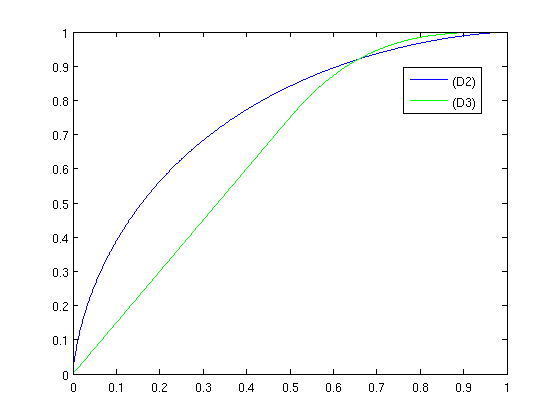
Figure 1: Df of false $p$-values in situation (D2) and (D3).

Note that (D1) may be replaced by

• distributed according to an df $F_{1}$ with $F_{1}(0.5)=1$

without changing the results of the simulation, because $0.5=\lambda=\lambda_{1}$ holds and given $(\hat{F}_{n}(t))_{t\geq\lambda}$ the adaptive SU test is just a BH test whose FDR only depends on the number of true null hypotheses. The results of the simulation are given in Table 1.

$\hat{n}_{0}$	(D1)	(D2)	(D3)
$\hat{n}_{0}(0.5)$	0.0501	0.0392	0.0354
$\sum_{i=1}^{3}\beta_{i}\hat{n}_{0}(\lambda_{i})$	0.0499	0.0432	0.0393
$\sum_{i=1}^{6}\hat{\beta}_{i}\hat{n}_{0}(\lambda_{i-1},\lambda_{i})$	0.0491	0.0437	0.0434

Table 1: FDR of the adaptive SU tests with Storey estimator (9), weighted Storey estimator (21) and dynamic estimator (27) which is introduced in Section 5.

The FDR of the classical BH test is here just $\frac{N_{0}}{n}\alpha=0.03$ which is enlarged by the adaptive tests. (D1) corresponds to a situation with maximal signal strength of false null hypotheses and (D4) includes many situations with large signal strength. In these situations, both estimators essentially lead to the same predetermined FDR level $\alpha$. (D2) and (D3) are situations with moderate signal strength. The approach of (D2) is often used to model true and false $p$-values and (D3) corresponds to a non-parametric approach. Here, the weighted Storey estimator is significantly superior to the Storey estimator. However, under the non-parametric approach it is easy to find distributions of false $p$-values, where the weighted Storey estimator is even more superior.

5 Dynamic approach

Let $0<\lambda=\lambda_{0}<\lambda_{1}<\ldots<\lambda_{k}=1$ and $\beta_{i}=\frac{\lambda_{i}-\lambda_{i-1}}{1-\lambda}$, $i=1,\ldots,k$. Then the primarily proposed estimator of Storey (2002, 2003) may be decomposed by

$$n\frac{1-\hat{F}_{n}(\lambda)}{1-\lambda}=n\sum_{i=1}^{k}\beta_{i}\frac{\hat{F}_{n}(\lambda_{i})-\hat{F}_{n}(\lambda_{i-1})}{\lambda_{i}-\lambda_{i-1}},$$ (24)

where the additional term $\frac{1}{n}$ of the Storey and generalized Storey estimators is omitted. Similar as in Section 4, the individual estimators $\hat{n}_{0}(\lambda_{i-1},\lambda_{i})$ and $n\frac{\hat{F}_{n}(\lambda_{i})-\hat{F}_{n}(\lambda_{i-1})}{\lambda_{i}-\lambda_{i-1}}$ may have an unknown bias depending on the distribution of false $p$-values. Furthermore, a small estimate of $N_{0}$ is desirable for a large power of the adaptive SU test. Therefore, a look at the data would be very helpful to adjust the the weights $\beta_{i}$ in this manner. Of course, FDR control may not be achieved by an arbitrary adjustment. But it turns out that a special data dependent weighting which uses the tail information of the ecdf $\hat{F}_{n}$ still leads to finite sample FDR control of the corresponding dynamic adaptive SU test and is not limited to the generalized Storey estimators.

Theorem 7.

Consider the BI Model, let $0<\lambda<\gamma_{1}\leq\ldots\leq\gamma_{k}\leq 1$ and $\mathcal{F}_{\gamma_{i}}=\sigma((\hat{F}_{n}(t))_{t\geq\gamma_{i}})$ be the generated $\sigma$-algebra, $i=1,\ldots,k$. Let $\hat{\beta}_{i}$ be non-negative, data dependent and $\mathcal{F}_{\gamma_{i}}$-measurable weights with $\sum_{i=1}^{k}\hat{\beta}_{i}=1$. Moreover, let $\widetilde{n}_{0}(\gamma_{i})$, $i=1,\ldots,k$, be $\mathcal{F}_{\lambda}$-measurable estimators of the form (11) which satisfy

$$E\left(\frac{V(\lambda)}{\widetilde{n}_{0}(\gamma_{i})}\Big{|}\mathcal{F}_{\gamma_{i}}\right)\leq\lambda,$$ (25)

including the generalized Storey estimators $\hat{n}_{0}(\lambda_{i},\gamma_{i})$ with $\lambda\leq\lambda_{i}<\gamma_{i}$. Then the estimator

$$\hat{n}_{0}=\sum_{i=1}^{k}\hat{\beta}_{i}\widetilde{n}_{0}(\gamma_{i})$$ (26)

satisfies (14) and the adaptive SU test with critical values (10) and estimator (26) has $FDR\leq\alpha$.

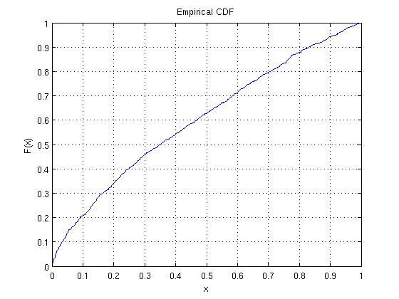
Figure 2: Likely ecdf of $p_{1},\ldots,p_{n}$ in situation (D2).

Below a practical adjustment of data driven weights $\hat{\beta}_{i}$ is motivated for the generalized Storey estimators (15). As illustration consider a simulation of situation (D2) of Section 4, where the ecdf $\hat{F}_{n}$ is presented in Figure 2. We are looking for an interval $[1-\delta,1]$, where $\hat{F}_{n}$ is most informative for the estimation of $N_{0}$. On this part the generalized Storey estimator $\hat{n}_{0}(\widetilde{\lambda},\widetilde{\gamma})$, $1-\delta\leq\widetilde{\lambda}<\widetilde{\gamma}<1$, may perform good. Since $\delta$ is unknown the interval $[\lambda,1]$ is first divided into small pieces $[\lambda_{i},\lambda_{i+1}]$. This observation motivates the following backwards data based dynamic adjustment of $\hat{\beta}_{i}$ which are related to the deterministic weights $\beta_{i}=\frac{\lambda_{i}-\lambda_{i-1}}{1-\lambda}$ used in (24). We are going to fill the last row of Table 1 for the following concrete adaptive weights $\hat{\beta}_{i}$ of that example. Fix in advance $\lambda=\lambda_{0}=0.5,\lambda_{1}=0.6,\lambda_{2}=0.7,\lambda_{3}=0.8,\lambda_{4}=0.9,\lambda_{5}=0.95,\lambda_{6}=1$ and let $\epsilon>0$ be a tuning parameter. The estimator

$$\hat{n}_{0}=\sum_{i=1}^{6}\hat{\beta}_{i}\hat{n}_{0}(\lambda_{i-1},\lambda_{i})$$ (27)

is established as follows. Based on the pre-weighting in (24) define

$$\hat{\beta}_{6}=\beta_{6}=\frac{\lambda_{6}-\lambda_{5}}{1-\lambda},\quad\mbox{and}\quad\hat{\beta}_{5}=\beta_{5}=\frac{\lambda_{5}-\lambda_{4}}{1-\lambda}.$$

The other weights are set as follows.
Case 1. Assume that there is an index $1\leq i\leq 4$ with

$$\hat{n}_{0}(\lambda_{i},\lambda_{i+1})>(1+\epsilon)\cdot\hat{n}_{0}(\lambda_{5},\lambda_{6})\quad$$ and (28)

$$\hat{n}_{0}(\lambda_{j},\lambda_{j+1})\leq(1+\epsilon)\cdot\hat{n}_{0}(\lambda_{5},\lambda_{6})\quad \mbox{for all }i<j\leq 4.$$ (29)

Then we put

$$\hat{\beta}_{i}=1-\sum_{j=i+1}^{6}\beta_{j},$$ (30)

$\hat{\beta}_{j}=\beta_{j}$ for $j>i$ and $\hat{\beta}_{1}=\ldots,\hat{\beta}_{i-1}=0$.
Case 2. If in case 1 there is no such index $i$ we may put $\hat{\beta}_{j}=\beta_{j}$ to be the pre-chosen weights for all $1\leq j\leq 6$.

The simulation of Section 4 is also conducted for the dynamic estimator (27) with tuning parameter $\epsilon=0.05$ and the results are given in Table 1. The corresponding dynamic adaptive SU test behaves almost like the adaptive SU test of the stationary approach, but shows significant advantages in the non-parametric case (D3).

Remark 8.

The construction of the dynamic weights is motivated by (24). Observe that the usual Storey estimator (9) mimics the “slope” of $t\mapsto\hat{F}_{n}(t)$ on the interval $[\lambda,1]$. The construction above splits that interval in smaller pieces with observed “slope” $\frac{\hat{F}_{n}(\lambda_{j})-\hat{F}_{n}(\lambda_{j-1})}{\lambda_{j}-\lambda_{j-1}}$ on the interval $[\lambda_{j-1},\lambda_{j}]$. In comparison with the Storey estimator the backwards stopping procedure will stop when the observed slope increases too much. In conclusion the procedure may be viewed as a data driven selection of an estimation region $[\lambda_{i-1},1]$. Note that the new SU tests have finite sample FDR control.

6 Adaptive SD tests

We now show that the results of the previous sections also hold for adaptive step down (SD) tests. Again, let $\hat{\alpha}_{i:n}$, $i=1,\ldots,n$, be data dependent critical values with $0=\hat{\alpha}_{0:n}<\hat{\alpha}_{1:n}\leq\ldots\leq\hat{\alpha}_{n:n}<1$. Then the adaptive SD test rejects all null hypotheses corresponding to the $p$-values $p_{i:n}$ which fulfill $p_{i:n}\leq\hat{\alpha}_{R_{SD}:n}$ with

$$R_{SD}=\max\{i:p_{j:n}\leq\hat{\alpha}_{j:n}\mbox{ for all }j\leq i\}$$ (31)

and the convention $\max\emptyset=0$. Note that $R_{SD}$ again denotes the the number of rejections. Furthermore, let

$$V_{SD}=\sum_{i=1}^{n}1\{p_{i}\leq\hat{\alpha}_{R_{SD}:n},H_{i}=0\}$$ (32)

be the number of falsely rejected true null hypotheses.

Theorem 9.

Consider the BI Model and the adaptive SD test with critical values (10) and estimator (11). Then

$$FDR=E\left(\frac{V_{SD}}{R_{SD}\vee 1}\right)\leq\frac{\alpha}{\lambda}E\left(\frac{V(\lambda)}{\hat{n}_{0}}\right)$$ (33)

holds. Moreover, the Theorems 2, 5 and 7 stay true if we replace adaptive SU test by adaptive SD test.

The adaptive SU tests described in Section 3-5 may also be carried out as adaptive SD tests with same critical values while still controlling the FDR at level $\alpha$. This has already be shown by Sarkar (2008) for the adaptive tests with estimators which may be treated by his FDR control condition. His methods include the Storey estimator (9), but exclude the generalized Storey estimators (15) with $\gamma_{1}<1$.

Remark 10.

Since the distribution of false $p$-values is arbitrary, ties may occur. If $p_{j_{1}:n}=\ldots=p_{j_{2}:n}$ holds for some $j_{1}<j_{2}$, then for the computation of $R_{SD}$ these $p$-values are basically compared to $\hat{\alpha}_{j_{1}:n}$ which is the smallest of the corresponding critical values. However, Theorem 9 also holds for the adaptive SD tests with data dependent critical values $\widetilde{\alpha}_{i:n}=\hat{\alpha}_{R(p_{i:n}):n}$, $i=1,\ldots,n$, where the $\hat{\alpha}_{i:n}$’s are given by (10) and $R(\cdot)$ is defined in (12). Then $p_{j_{1}:n}=\ldots=p_{j_{2}:n}$ are compared to $\alpha_{j_{2}:n}$ which is the largest of the corresponding critical values. The proof of this remark is included in the proof of Theorem 9.

7 Converse Benjamini Hochberg Theorem

In this section we show under mild assumptions that the SU test of Benjamini and Hochberg (1995) is the only SU test with $FDR=\frac{E(N_{0})}{n}\alpha$ under the BI Model. This converse BH-Theorem may be of interest when new testing procedures are supposed to be designed. The converse theorem relies on the following submodel of the BI Model given by Efron’s mixture model (34).

• The possible false $p$-values $\xi_{1},\ldots,\xi_{n}$ are i.i.d. according to an unknown distribution function $F_{1}$ with Lebesgue density. In addition, let $\xi_{1}$ be stochastically smaller than a uniformly distributed $p$-value on the unit interval, i.e. $F_{1}(t)\geq t$, $0\leq t\leq 1$.

• The random variables $H_{1},\ldots,H_{n}$ are Bernoulli variables and independent of $(\xi_{i})_{i\leq n}$. Furthermore, let the range of probabilities $P(H_{1}=0)$ covers an interval $I\subset(0,1)$ with non-empty interior.

Thus, the $p$-values $p_{1},\ldots,p_{n}$ are i.i.d. according to the distribution function

$$F(t)=P(H_{1}=0)\cdot t+P(H_{1}=1)\cdot F_{1}(t),\quad t\in[0,1].$$ (34)

Theorem 11.

Consider an adaptive SU test with critical values (10) and estimator (11).
(a) Suppose that $FDR=E(N_{0})c$ holds for some constant $0<c<\frac{1}{n}$ for all distributions of the BI Model which satisfy (C1) and (C2). Then the sets of critical values have already the form

$$\hat{\alpha}_{i:n}=\frac{i}{n}\alpha\mbox{ almost surely},$$ (35)

for $i=1,\ldots,n$, where $\alpha=nc$.
(b) Suppose that $FDR=E(N_{0})c$ holds for some constant $0<c<\frac{1}{n}$ for all distributions of the BI Model with fixed $N_{0}=1$ and (C1). Then (35) holds again.

Remark 12.

(a) There is no hope to obtain exact $FDR=\alpha$ for the adaptive SU tests for all distributions of the BI Model. The BH test is the only SU test with FDR which is “distribution free” with respect to the distribution of false $p$-values.
(b) In case of deterministic critical values $0<\alpha_{1:n}\leq\ldots\leq\alpha_{n:n}<1$ we may choose $\lambda=\alpha_{n:n}$ and Theorem 11 applies.

Suppose that $i\mapsto\frac{\alpha_{i:n}}{i}$ is non-decreasing. Then Benjamini and Yekutieli (2001) proved that the FDR is non-decreasing when the distribution $F_{1}$ of the false $p$-values becomes stochastically smaller (and the other way around when $\frac{\alpha_{i:n}}{i}$ does not increase). In these cases Theorem 11 is not so surprising. However, the present result holds in general without any further monotonicity assumption of that kind and it is also true for our data dependent critical values.

8 Proofs

Proof of Theorem 1. Conditioned under the generated $\sigma$-algebra

$$\mathcal{F}_{\lambda}=\sigma(H_{i},1\{p_{i}\leq s\}:s\geq\lambda,1\leq i\leq n),$$

the random variables $H_{i}$ and $1\{p_{i}\leq s\}$, $i=1,\ldots,n$, $s\geq t$, and in particular $n\hat{F}_{n}(s)=R(s)$, $s\geq\lambda$, can be treated as fixed deterministic values, due to measurability arguments. Under this condition we have exactly $V(\lambda)$ true $p$-values smaller or equal to $\lambda$, where $V(\lambda)$ is a fixed number too. Without restriction we assume $n_{0}\geq V(\lambda)>0$ since everything is obviously fine for the excluded cases. Let us now consider new rescaled $p$-values $q_{i}$, $i=1,\ldots,R(\lambda)$ defined by

$$q_{i:R(\lambda)}:=\frac{p_{i:n}}{\lambda},\quad i=1,\ldots,R(\lambda).$$

The new $p$-values $q_{i}$ corresponding to true null hypotheses are again i.i.d. and uniformly distributed on $(0,1)$ and independent from the rest of the $p$-values $q_{i}$ corresponding to false null hypotheses under the above condition. The exact positions of the $V(\lambda)$ true $p$-values in $(q_{1},\ldots,q_{R(\lambda)})$ does not matter for our considerations. We now apply the BH Theorem for SU tests with critical values

$$\alpha_{i:R(\lambda)}^{(q)}:=\frac{i}{R(\lambda)}\alpha^{\prime}\quad\mbox{and }\alpha^{\prime}:=\frac{R(\lambda)}{\lambda\hat{n}_{0}}\alpha$$

on the $q$’s. The data dependent level $\alpha^{\prime}$ only depends by assumption (11) on the information given by $\mathcal{F}_{\lambda}$. Conditionally under $\mathcal{F}_{\lambda}$ we have a regular non data dependent SU procedure on the $q$’s. Let $R_{q}$ and $V_{q}$ denote the number of rejections and false rejections respectively by the above SU test. Observe that

$$E\left(\frac{V_{q}}{R_{q}}\Big{|}\mathcal{F}_{\lambda}\right)=\frac{V(\lambda)}{R(\lambda)}\min(\alpha^{\prime},1)$$ (36)

holds by the BH Theorem. Obviously (36) is $\frac{V(\lambda)}{R(\lambda)}$ in case $\alpha^{\prime}\geq 1$.

Now observe that

$$R_{q} = \max\{i\leq R(\lambda)\,:\,q_{i:R(\lambda)}\leq\alpha_{i:R(\lambda)}^{(q)}\}$$

$$= \max\left\{i\leq R(\lambda)\,:\,\frac{p_{i:n}}{\lambda}\leq\frac{i}{R(\lambda)}\frac{R(\lambda)}{\lambda\hat{n}_{0}}\alpha\right\}$$

$$= \max\left\{i\leq n\,:\,p_{i:n}\leq\left(\frac{i}{\hat{n}_{0}}\alpha\right)\wedge\lambda\right\}=R$$

and hence $V_{q}=V$ since both tests, belonging to $R$ and $R_{q}$, are rejecting the same hypotheses. Thus, by (36) we get

$$E\left(\frac{V}{R}\right) = E\left(E\left(\frac{V}{R}\,\Big{|}\mathcal{F}_{\lambda}\right)\right)=E\left(E\left(\frac{V_{q}}{R_{q}}\,\Big{|}\mathcal{F}_{\lambda}\right)\right)$$

$$= E\left(\frac{V(\lambda)}{R(\lambda)}\min(\alpha^{\prime},1)\right)=\frac{\alpha}{\lambda}E\left(V(\lambda)\min\left\{\frac{1}{\hat{n}_{0}},\frac{\lambda}{R(\lambda)\alpha}\right\}\right).$$

$\hfill\square$

Proof of Theorem 2. First let us introduce the following simplifying notation

$$V(t) :=n_{0}(t):=\#\{p_{i}\leq t\,:\,p_{i}\mbox{ true}\}$$

$$S(t) :=n_{1}(t):=\#\{p_{i}\leq t\,:\,p_{i}\mbox{ false}\},\quad 0\leq t\leq 1$$

and similar to the proof of Theorem 1 let us condition under

$$\mathcal{F}_{\gamma_{1}}=\sigma(H_{i},1\{p_{i}\leq s\}:s\geq\gamma_{1},1\leq i\leq n).$$

Whereas $n_{0}(t)$ and $n_{1}(t)$ refer to known fixed values under the present condition, $V(t)$ and $S(t)$ are still random. Since $n_{1}(\gamma_{1})-S(\lambda_{1})\geq 0$ we obtain

$$E\left(\frac{V(\lambda)}{n(\hat{F}_{n}(\gamma_{1})-\hat{F}_{n}(\lambda_{1})+\frac{1}{n})}\Big{|}\mathcal{F}_{\lambda}\right)$$ (37)

$$=E\left(\frac{V(\lambda)}{n_{0}(\gamma_{1})+1-V(\lambda)-(V(\lambda_{1})-V(\lambda))+n_{1}(\gamma_{1})-S(\lambda_{1})}\Big{|}\mathcal{F}_{\lambda}\right)$$ (38)

$$\leq E\left(\frac{V(\lambda)}{n_{0}(\gamma_{1})+1-V(\lambda)-(V(\lambda_{1})-V(\lambda))}\Big{|}\mathcal{F}_{\lambda}\right).$$ (39)

The random vector $(V(\lambda),V(\lambda_{1})-V(\lambda),V(\gamma_{1})-V(\lambda_{1}))$ is distributed according to the multinomial distribution $\mathcal{M}\left(n_{0}(\gamma_{1}),\frac{\lambda}{\gamma_{1}},\frac{\lambda_{1}-\lambda}{\gamma_{1}},\frac{\gamma_{1}-\lambda_{1}}{\gamma_{1}}\right)$ under our conditions. The subsequent Lemma yields

$$(\ref{StarErsatz})=\frac{\lambda}{\gamma_{1}-\lambda_{1}}\left(1-\left(\frac{\lambda_{1}}{\gamma_{1}}\right)^{n_{0}(\gamma_{1})}\right)\leq\frac{\lambda}{\gamma_{1}-\lambda_{1}}.$$

Integration now gives

$$\quad\quad\quad\quad E\left(\frac{V(\lambda)}{n(\hat{F}_{n}(\gamma_{1})-\hat{F}_{n}(\lambda_{1})+\frac{1}{n})}\Big{|}(\hat{F}_{n}(t))_{t\geq\gamma_{1}}\right)\leq\frac{\lambda}{\gamma_{1}-\lambda_{1}}.\quad\quad\quad\quad\quad\square$$

Lemma 13.

Let $(V_{1},V_{2},V_{3})$ be distributed according to the multinomial distribution $\mathcal{M}(n,p_{1},p_{2},p_{3})$ with $p_{3}>0$ and $n\geq 0$. Then we have

$$E\left(\frac{V_{1}}{n+1-V_{1}-V_{2}}\right)=\frac{p_{1}}{p_{3}}(1-(p_{1}+p_{2})^{n}).$$ (40)

Proof. A simple calculation shows

$$E\left(\frac{V_{1}}{n+1-V_{1}-V_{2}}\right)$$

$$=\sum_{{k_{1}>0,\ k_{2}\geq 0},\ {k_{1}+k_{2}\leq n}}\frac{n!}{(k_{1}-1)!k_{2}!(n+1-k_{1}-k_{2})!}p_{1}^{k_{1}}p_{2}^{k_{2}}p_{3}^{n-k_{1}-k_{2}}$$

$$=\frac{p_{1}}{p_{3}}\cdot\sum_{{j,k_{2}\geq 0},\ {j+k_{2}\leq n-1}}\frac{n!}{j!k_{2}!(n-j-k_{2})!}p_{1}^{j}p_{2}^{k_{2}}p_{3}^{n-j-k_{2}}.$$

The last equality follows from the substitution $j=k_{1}-1$. Observe that the last term adds the probabilities of the multinomial distribution times a constant factor, so extending the missing probabilities yields that the last term equals

$$\frac{p_{1}}{p_{3}}\cdot\left(1-\sum_{j+k_{2}=n}\frac{n!}{j!k_{2}!(n-j-k_{2})!}p_{1}^{j}p_{2}^{k_{2}}p_{3}^{n-j-k_{2}}\right)$$

$$=\frac{p_{1}}{p_{3}}\cdot\left(1-\sum_{j=0}^{n}\frac{n!}{j!(n-j)!}p_{1}^{j}p_{2}^{n-j}\right)=\frac{p_{1}}{p_{3}}\cdot\left(1-(p_{1}+p_{2})^{n}\right).\quad\quad\square$$

Proof of Lemma 4. Let us condition under $N_{0}=n_{0}>0$. Without restrictions assume that the $p$-values $p_{1},\ldots,p_{n_{0}}$ belong to true null hypotheses. By (11) we have $\hat{n}_{0}^{(1)}=\hat{n}_{0}$ on $\{p_{1}\leq\lambda\}$ and thus,

$$E\left(\frac{V(\lambda)}{\hat{n}_{0}}\Big{|}N_{0}=n_{0}\right)=\sum_{i=1}^{n_{0}}E\left(\frac{1\{p_{i}\leq\lambda\}}{\hat{n}_{0}}\Big{|}N_{0}=n_{0}\right)$$

$$=n_{0}E\left(\frac{1\{p_{1}\leq\lambda\}}{\hat{n}_{0}}\Big{|}N_{0}=n_{0}\right)=n_{0}E\left(\frac{1\{p_{1}\leq\lambda\}}{\hat{n}_{0}^{(1)}}\Big{|}N_{0}=n_{0}\right)$$

$$=\lambda E\left(\frac{n_{0}}{\hat{n}_{0}^{(1)}}\Big{|}N_{0}=n_{0}\right).$$

The last equality holds because of the independence of $p_{1}$ and $\hat{n}_{0}^{(1)}$, where $p_{1}$ is uniformly distributed on $(0,1)$. There is nothing to show for $N_{0}=0$ and hence integration yields the assertion. $\hfill\square$

Proof of Corollary 5. The estimator $\hat{n}_{0}$ given in (21) is a convex combination. Thus, by Theorem 2 with $\gamma_{i}=1$ we obtain

$$\quad\quad\quad E\left(\frac{V(\lambda)}{\sum_{i=1}^{k}\beta_{i}\hat{n}_{0,i}}\right)\leq\sum_{i=1}^{k}\beta_{i}E\left(\frac{V(\lambda)}{\hat{n}_{0,i}}\right)\leq\sum_{i=1}^{k}\beta_{i}\lambda=\lambda.\quad\quad\quad\quad\square$$

Proof of Theorem 7. Along the lines of the proof of the stationary approach (Corollary 5) observe that

$$\frac{V(\lambda)}{\sum_{i=1}^{k}\hat{\beta}_{i}\widetilde{n}_{0}(\gamma_{i})}\leq\sum_{i=1}^{k}\hat{\beta}_{i}\frac{V(\lambda)}{\widetilde{n}_{0}(\gamma_{i})}$$

holds for fixed $p$-values. Since $\hat{\beta}_{i}$ is $\mathcal{F}_{\gamma_{i}}$ measurable and (25), by taking conditional expectations we finally get

$$\quad E\left(\frac{V(\lambda)}{\hat{n}_{0}}\right) \leq E\left(\sum_{i=1}^{k}\hat{\beta}_{i}\frac{V(\lambda)}{\widetilde{n}_{0}(\gamma_{i})}\right)=E\left(\sum_{i=1}^{k}\hat{\beta}_{i}E\left(\frac{V(\lambda)}{\widetilde{n}_{0}(\gamma_{i})}\Big{|}\mathcal{F}_{\gamma_{i}}\right)\right)$$

$$\leq E\left(\sum_{i=1}^{k}\hat{\beta}_{i}\lambda\right)=\lambda.\hskip 170.71652pt\square$$

Proof of Theorem 9. (I) The proof is first done for the BH critical values $\alpha_{i:n}=\frac{i}{n}\alpha$ where also $\alpha\geq 1$ is allowed for SD tests at this point. For each $\alpha>0$ we will now prove

$$E\left(\frac{V_{SD}}{R_{SD}}\right)\leq\frac{E(N)}{n}\alpha$$ (41)

for the BH SD test. Under the BI Model we can condition under $H_{1},\ldots,H_{n}$ which are assumed to be fixed throughout. Then

$$\begin{array}[]{ll}E\left(\frac{V_{SD}}{R_{SD}}\Big{|}H_{1},\ldots,H_{n}\right)&=\sum_{i:H_{i}=0}E\left(\frac{1\{p_{i}\leq\alpha_{R_{SD}:n}\}}{R_{SD}}\Big{|}H_{1},\ldots,H_{n}\right)\\ &=N_{0}E\left(\frac{1\{p_{1}\leq\alpha_{R_{SD}:n}\}}{R_{SD}}\Big{|}H_{1},\ldots,H_{n}\right),\end{array}$$ (42)

where $p_{1}$ is assumed to be a true $p$-value, without restrictions. Let $p=(p_{1},\ldots,p_{n})$ be the vector of p-values and $p^{(1)}=(0,p_{2},\ldots,p_{n})$ the vector of p-values, where the first true $p$-value $p_{1}$ is decreased to zero. Simple calculations show that $R_{SD}(p)=R_{SD}(p^{(1)})$ holds on the set $\{p_{1}\leq\alpha_{R_{SD}(p):n}\}$. Observe when $p_{1}$ is rejected and then $p_{1}$ could also be zero. Moreover we have $\{p_{1}\leq\alpha_{R_{SD}(p):n}\}\subset\{p_{1}\leq\alpha_{R_{SD}(p^{(1)}):n}\}$ in any case. Thus,

$$E\left(\frac{1\{p_{1}\leq\alpha_{R_{SD}:n}\}}{R_{SD}}\Big{|}H_{1},\ldots,H_{n}\right) \leq E\left(\frac{1\{p_{1}\leq\alpha_{R_{SD}(p^{(1)}):n}\}}{R_{SD}(p^{(1)})}\Big{|}H_{1},\ldots,H_{n}\right)$$

$$\leq E\left(\frac{\alpha_{R_{SD}(p^{(1)}):n}}{R_{SD}(p^{(1)})}\Big{|}H_{1},\ldots,H_{n}\right)=\frac{\alpha}{n}$$

by the independence of $p_{1}$ and $R_{SD}(p^{(1)})$ and Fubini’s theorem.
(II) Inequality (41) also holds for the modified data-dependent critical values

$$\widetilde{\alpha}_{i:n}^{\prime}:=\alpha_{R(p_{i:n}):n}=\hat{F}_{n}(p_{i:n})\alpha.$$

The same arguments of (I) can be applied by simply replacing $\alpha_{\,\cdot\,:n}$ by $\widetilde{\alpha}_{\,\cdot\,:n}$ and observing that $R_{SD}(p^{(1)})=n\hat{F}_{n}(p_{R_{SD}(p^{(1)}):n})$ holds.
(III) As in the proof of Theorem 1 we may condition under $\mathcal{F}_{\lambda}$. If we now use the inequality of (I) and (II) for the procedures, then Lemma 9 follows from slightly adapted arguments given in the proof of Theorem 1 and crossing over to inequalities. The arguments hold for $\hat{\alpha}_{i:n}$ as well as for $\widetilde{\alpha}_{i:n}$. The only difference for the SD case is that the upper bound of (36) is $\frac{V(\lambda)}{R(\lambda)}\alpha^{\prime}$ with the inequality “$\leq$” instead of “=” in general. Furthermore $R_{q,SD}=R_{SD}$ still holds for both tests by an analogue argument for SD tests. $\hfill\square$

Proof of Theorem 11. This proof uses results for complete statistical models which can be found in Lehmann and Romano (2005) and Pfanzagl (1994). Our assumptions imply

$$\int\left(E\left(\frac{V}{R}\Big{|}N_{0}=n_{0}\right)-cn_{0}\right)\mathcal{L}(N_{0})(dn_{0})=0$$

for all distributions specified in (C1) and (C2). Observe that $\mathcal{L}(N_{0})$ is a binomial distribution. Thus,

$$E\left(\frac{V}{R}\Big{|}N_{0}=n_{0}\right)-cn_{0}=0$$

holds for all $n_{0}\in\{0,\ldots,n\}$ since $N_{0}$ is a complete statistic for the exponential family of binomials. Next we focus on $N_{0}=1$ and the proofs of (a) and (b) run parallel. Without restrictions we may assume that the true $p$-value is $p_{1}$ given by $U_{1}$. In that case $V$ and $R$ depend on the outcomes $(p_{1},\ldots,p_{n})=(U_{1},\xi_{2},\ldots,\xi_{n})$, where $V(p_{1},\ldots,p_{n})=V(U_{1},\xi_{1:n-1},\ldots,\xi_{n-1:n-1})$ holds and similarly for $R$. Note that here $\xi_{1:n-1},\ldots,\xi_{n-1:n-1}$ denote the order statistics of $\xi_{2},\ldots,\xi_{n}$. Furthermore, put $\alpha=nc$. It is easy to see that $\alpha<1$ holds and the model includes i.i.d. uniformly on $(0,1)$ distributed $\xi_{i}$. Then we have $nE(\frac{V}{R}|N_{0}=1)=E(\frac{R}{R}1\{R>0\})=P(R>0)<1$ in both cases. Now we have

$$0 = E\left(\frac{V}{R}\Big{|}N_{0}=1\right)-\frac{\alpha}{n}=E\left(\frac{V(U_{1},\xi_{2},\ldots,\xi_{n})}{R(U_{1},\xi_{2},\ldots,\xi_{n})}-\frac{\alpha}{n}\right)$$

$$= \int\int_{0}^{1}\left(\frac{V(U_{1},(\xi_{i:n-1})_{i\leq n-1})}{R(U_{1},(\xi_{i:n-1})_{i\leq n-1})}-\frac{\alpha}{n}\right)$$

$$\hskip 113.81102ptdU_{1}\ \mathcal{L}((\xi_{i:n-1})_{i\leq n-1})d((\xi_{i:n-1})_{i\leq n-1}).$$

Observe that the family of distributions of $\mathcal{L}(\xi_{1})$ is convex and complete in the sense of Pfanzagl (1994) Theorem 1.5.10. Thus, the family of order statistics $(\xi_{i:n-1})_{i\leq n-1}$ is also complete and

$$\int_{0}^{1}\frac{V(U_{1},(\xi_{i:n-1})_{i\leq n-1})}{R(U_{1},(\xi_{i:n-1})_{i\leq n-1})}\ dU_{1}=\frac{\alpha}{n}$$ (43)

holds $\mathcal{L}((\xi_{i:n-1})_{i\leq n-1})$ almost surely. Consider first deterministic $\alpha_{i:n}$. Let $p=(p_{1},\ldots,p_{n})$ be the vector of p-values and $p^{(1)}=(0,p_{2},\ldots,p_{n})$ the vector of p-values, where the first true $p$-value $p_{1}$ is decreased to zero. Simple calculations show that $R(p)=R(p^{(1)})$ holds on the set $\{p_{1}\leq\alpha_{R(p):n}\}$. Observe when $p_{1}$ is rejected and then $p_{1}$ could also be zero. Moreover, we have $\{p_{1}\leq\alpha_{R(p):n}\}=\{p_{1}\leq\alpha_{R(p^{(1)}):n}\}$ in any case. The left hand side of (43) is thus equal to

$$\int_{0}^{1}\frac{1\{p_{1}\leq\alpha_{R:n}\}}{R}\ dp_{1}=\frac{\alpha_{R(p^{(1)}):n}}{R(p^{(1)})}.$$ (44)

The same arguments apply to the data driven critical values $\hat{\alpha}_{i:n}$. We have only to take $p_{1}\leq\lambda$ into account. In this case we see that $\hat{n}_{0}(p)=\hat{n}_{0}(p^{(1)})$ does not change since $(\hat{F}_{n}(t))_{t\geq\lambda}$ is the same for $p$ and $p^{(1)}$. On $\{p_{1}\leq\lambda\}$ the $\hat{\alpha}_{i:n}$ can be considered to be deterministic and (44) also holds $\lambda\!\!\lambda_{(0,1)}^{n-1}$ $a.s$. It is easy to see that the set $\{R(p^{(1)})=j\}$ has positive probability for each value $1\leq j\leq n$ under at least one distribution of model (C1). Therefore, consider uniformly on $(0,1)$ distributed false $p$-values and observe that

$$\{p_{j:n}\leq\alpha_{j:n},\,p_{j+1:n}>\alpha_{n:n}\}\subset\{R(p^{(1)})=j\}$$

holds for deterministic critical values and

$$\{p_{j:n}\leq\hat{\alpha}_{j:n},\,p_{j+1:n}>\lambda\}\subset\{R(p^{(1)})=j\}$$

for our data driven critical values. From (43) and (44) we conclude the equality $\frac{\alpha_{j:n}}{j}=\frac{\alpha}{n}$ for all $1\leq j\leq n.$ $\hfill\square$

References

- Benjamini and Hochberg (1995) Benjamini, Y., Hochberg, Y., 1995. Controlling the false discovery rate: a practical and powerful approach to multiple testing. J. Roy. Statist. Soc. Ser. B 57 (1), 289–300.
- Benjamini and Hochberg (2000) Benjamini, Y., Hochberg, Y., 2000. On the adaptive control of the false discovery rate in multiple testing with independent statistics. J. Educ. Behav. Statist. 25 (1), 60–83.
- Benjamini et al. (2006) Benjamini, Y., Krieger, A. M., Yekutieli, D., 2006. Adaptive linear step-up procedures that control the false discovery rate. Biometrika 93 (3), 491–507.
- Benjamini and Yekutieli (2001) Benjamini, Y., Yekutieli, D., 2001. The control of the false discovery rate in multiple testing under dependency. Ann. Statist. 29 (4), 1165–1188.
- Blanchard and Roquain (2009) Blanchard, G., Roquain, E., 2009. Adaptive false discovery rate control under independence and dependence. J. Mach. Learn. Res. 10, 2837–2871.
- Celisse and Robin (2010) Celisse, A., Robin, S., 2010. A cross-validation based estimation of the proportion of true null hypotheses. J. Statist. Plann. Inference 140 (11), 3132–3147.
- Chen and Doerge (2012) Chen, X., Doerge, R. W., April 2012. Generalized estimators for multiple testing: proportion of true nulls and false discovery rate. Tech. rep., Department of Statistics, Purdue University, West Lafayette, USA.
- Efron et al. (2001) Efron, B., Tibshirani, R., Storey, J. D., Tusher, V., 2001. Empirical Bayes analysis of a microarray experiment. J. Amer. Statist. Assoc. 96 (456), 1151–1160.
- Finner and Gontscharuk (2009) Finner, H., Gontscharuk, V., 2009. Controlling the familywise error rate with plug-in estimator for the proportion of true null hypotheses. J. R. Stat. Soc. Ser. B Stat. Methodol. 71 (5), 1031–1048.
- Finner and Roters (2001) Finner, H., Roters, M., 2001. On the false discovery rate and expected type I errors. Biom. J. 43 (8), 985–1005.
- Heesen (2014) Heesen, P., 2014. Adaptive step up tests for the false discovery rate (FDR) under independence and dependence. Ph.D. thesis, Heinrich-Heine-Universität Düsseldorf, Germany.
- Langaas et al. (2005) Langaas, M., Lindqvist, B. H., Ferkingstad, E., 2005. Estimating the proportion of true null hypotheses, with application to DNA microarray data. J. R. Stat. Soc. Ser. B Stat. Methodol. 67 (4), 555–572.
- Lehmann and Romano (2005) Lehmann, E. L., Romano, J. P., 2005. Testing statistical hypotheses, 3rd Edition. Springer Texts in Statistics. Springer, New York.
- Liang and Nettleton (2012) Liang, K., Nettleton, D., 2012. Adaptive and dynamic adaptive procedures for false discovery rate control and estimation. J. R. Stat. Soc. Ser. B. Stat. Methodol. 74 (1), 163–182.
- Meinshausen and Rice (2006) Meinshausen, N., Rice, J., 2006. Estimating the proportion of false null hypotheses among a large number of independently tested hypotheses. Ann. Statist. 34 (1), 373–393.
- Pfanzagl (1994) Pfanzagl, J., 1994. Parametric statistical theory. de Gruyter Textbook. Walter de Gruyter & Co., Berlin, with the assistance of R. Hamböker.
- Sarkar (2002) Sarkar, S. K., 2002. Some results on false discovery rate in stepwise multiple testing procedures. Ann. Statist. 30 (1), 239–257.
- Sarkar (2008) Sarkar, S. K., 2008. On methods controlling the false discovery rate. Sankhyā 70 (2, Ser. A), 135–168.
- Sarkar et al. (2012) Sarkar, S. K., Guo, W., Finner, H., 2012. On adaptive procedures controlling the familywise error rate. J. Statist. Plann. Inference 142 (1), 65–78.
- Schweder and Spjotvoll (1982) Schweder, T., Spjotvoll, E., 1982. Plots of p-values to evaluate many tests simultaneously. Biometrika 69 (3), 493–502.
- Simes (1986) Simes, R. J., 1986. An improved bonferroni procedure for multiple tests of significance. Biometrika 73 (3), 751–754.
- Storey (2002) Storey, J. D., 2002. A direct approach to false discovery rates. J. R. Stat. Soc. Ser. B Stat. Methodol. 64 (3), 479–498.
- Storey (2003) Storey, J. D., 2003. The positive false discovery rate: a Bayesian interpretation and the -value. Ann. Statist. 31 (6), 2013–2035.
- Storey et al. (2004) Storey, J. D., Taylor, J. E., Siegmund, D., 2004. Strong control, conservative point estimation and simultaneous conservative consistency of false discovery rates: a unified approach. J. R. Stat. Soc. Ser. B Stat. Methodol. 66 (1), 187–205.
- Storey and Tibshirani (2003) Storey, J. D., Tibshirani, R., 2003. Statistical significance for genomewide studies. PNAS 100 (16), 9440–9445.
- Zeisel et al. (2011) Zeisel, A., Zuk, O., Domany, E., 2011. FDR control with adaptive procedures and FDR monotonicity. Ann. Appl. Stat. 5 (2A), 943–968.