Oscillation modes in the rapidly rotating Slowly Pulsating B-type star $\mn@boldsymbol{\mu}$ Eridani

Abstract

We present results of a search for identification of modes responsible for the six most significant frequency peaks detected in the rapidly rotating SPB star $\mu$ Eridani. All published and some unpublished photometric data are used in our new analysis. The mode identification is carried out with the method developed by Daszyńska-Daszkiewicz et al. employing the phases and amplitudes from multi-band photometric data and relying on the traditional approximation for the treatment of oscillations in rotating stars. Models consistent with the observed mean parameters are considered. For the five frequency peaks, the candidates for the identifications are searched amongst unstable modes. In the case of the third frequency, which is an exact multiple of the orbital frequency, this condition is relaxed. The systematic search is continued up to a harmonic degree $\ell=6$. Determination of the angular numbers, $(\ell,m)$, is done simultaneously with the rotation rate, $V_{\rm rot}$, and the inclination angle, $i$, constrained by the spectroscopic data on the projected rotational velocity, $V_{\rm rot}\sin i$, which is assumed constant. All the peaks may be accounted for with g-modes of high radial orders and the degrees $\ell\leq 6$. There are differences in some identifications between the models. For the two lowest–amplitude peaks the identifications are not unique. Nonetheless, the equatorial velocity is constrained to a narrow range of (135, 140) km/s. Our work presents the first application of the photometric method of mode identification in the framework of the traditional approximation and we believe that it opens a new promising direction in studies of SPB stars.

1 Introduction

Variability with a few periods of the order of one day is frequently observed in main-sequence B-type stars (e.g. De Cat, 2007). Objects exhibiting only these slow oscillations are now called Slowly Pulsating B-type stars (SPB) and are found in the spectral-type range of B3-B8. It is commonly believed that this variability is due to excitation of high-order g-modes. Such modes are also invoked as an explanation of low-frequency variations observed in certain $\beta$ Cephei stars. Linear non-adiabatic calculations predict excitation of high-order g-modes in a wide range of main sequence B-type stars. However, difficulties in explaining in this way long-period variability in certain objects have been noted.

In several stars, observations from space by the CoRoT and Kepler missions led to the detection of a large number of frequency peaks which may be associated with g-modes. However, mode identification for individual peaks seems a formidable task. A method based on a search for equidistant spacing in period, that has been successfully used in the application to white dwarfs, was tried for the CoRoT target HD50230 by Degroote et al. (2010). The authors found a sequence of eight modes with a remarkably constant separation, much more so than in relevant models (Dziembowski, Moskalik & Pamyatnykh, 1993; Aerts & Dupret, 2012). In the same frequency range there were over 100 frequencies (some of much higher S/N than most of those forming the sequence) for which no plausible interpretation was offered so far (Szewczuk, Daszyńska-Daszkiewicz & Dziembowski, 2014). In an attempt to explain the oscillation spectrum of another CoRoT target, HD 43317, Savonije (2013) also could not account for the equidistant spacing reported by Pápics et al. (2012). Patterns in oscillation spectra apparently do not yield a key toward deciphering information on excited modes in SPB stars. We need to know more about mode selection in these stars. Perhaps we may learn something new about it from ground-based observations, which yield much fewer frequency peaks than the ones from space, but much more information about each of them that would enable mode identification. In this respect, the SPB star $\mu$ Eri appears to be the best choice.

A large number of three-passband photometric data for this star have been collected during two multisite campaigns (MSC) aimed at the $\beta$ Cep variable $\nu$ Eri, 2002-2003 MSC (Handler et al., 2004) and 2003-2004 MSC (Jerzykiewicz et al., 2005, hereafter J2005). The star has been used as one of two comparison stars in both campaigns. The analysis of the 2002-2003 MSC data by Handler et al. (2004) revealed a variability of $\mu$ Eri with a frequency of 0.616 c/d. However, the authors were not able to decide what is the origin of this variation: pulsation or rotational modulation. The analysis of the extensive data set from both campaigns presented in J2005 led to the detection of five additional significant peaks in the g-mode frequency range typical for SPB stars and an unambiguous classification of $\mu$ Eri.

Additional three-colour data were recently obtained by one of us (GH). These and the MSC data were employed in the mode identification presented in our work. Photometry with the MOST micro-satellite (Jerzykiewicz et al., 2013, hereafter J2013) was also used in frequency determination in Section 2.3. Unfortunately, spectroscopic observations reported in the same paper yielded only the upper bound on radial velocity variations. However, these observations were used to constrain parameters of the star; this, as we will see later in the paper, is essential for mode identification.

All data used in our work are presented in the next section. We also provide information on the mean physical parameters of the star and describe its models which will be used in the subsequent sections.

In Section 3, we confront frequencies of the peaks with instability ranges determined in one of the selected models. We use the condition of mode instability as a requirement for its possible association with an observed frequency. Mode visibility is another factor limiting the set of modes for possible identification. This matter is discussed in Section 4.

Section 5 is devoted to an analysis of the data on the amplitudes and phases of the six peaks determined in three photometric passbands. The aim is to determine the harmonic degree, $\ell$, and the azimuthal order, $m$, of the observed modes simultaneously with constraints on the stellar rotation rate, assuming that it is uniform. The method, which employs the traditional approximation, has been described in detail by Daszyńska-Daszkiewicz, Dziembowski & Pamyatnykh (2007a, hereafter D07a) and here we give only its brief outline.

We have not attempted to constrain a stellar model by fitting calculated frequencies to observations because it would not make sense in view of the approximation adopted in treating the effects of rotation and high density of the calculated oscillation spectra related to high radial orders of the excited modes. Our primary goal is to learn something about mode selection in SPB stars. We believe that this is essential for understanding complicated oscillation spectra from the space missions. The discussion in the final section is focused on this issue.

2 $\mn@boldsymbol{\mu}$ Eridani

$\mu$ Eridani (HD 30211) is a bright ($V={}$4 mag) B5 IV star. It is certainly not a slow rotator. J2013 provide two independent estimates of the projected equatorial velocity of rotation, $V_{\rm rot}\sin i={}$130$\,\pm\,$3 and 136$\,\pm\,$6 km/s. It has been known since a long time (Frost & Lee, 1910) that the star is the primary in a single-lined spectroscopic binary system but only J2005 detected shallow eclipses. This is a well detached system with the orbital period $P_{\rm orb}={}$7.38090 d and eccentricity $e={}$0.344 (J2013). Hence, we can neither assume synchronized rotation nor parallel rotation and orbital axes. Thus, mode identification must be done simultaneously with the determination of the inclination angle.

2.1 Mean parameters and evolutionary models

We adopted after J2013 $\log T_{\rm eff}={}$4.195$\,\pm\,$0.013 and $\log L/{\rm L}_{\sun}={}$3.280$\,\pm\,$0.040 for the effective temperature and luminosity of $\mu$ Eri. These values were found from the mean Strömgren photometric indexes and the revised value of the Hipparcos parallax (van Leeuwen, 2007). From their own spectroscopic data, J2013 found a metal abundance close to solar. They also determined the mean density of the star, $\bar{\rho}={}$0.0348$\,\pm\,$0.0032 g/cm³ from the orbital parameters.

The above-mentioned values of $\log T_{\rm eff}$, $\log L/{\rm L}_{\sun}$ and $\bar{\rho}$ imply a mass $M\approx{}$6.0 M_☉ and a radius $R\approx{}$6.1 R_☉, hence the break-up velocity amounts to $V_{\rm rot}^{\rm crit}\approx\sqrt{\frac{GM}{R}}\approx{}$ 430 km/s and the corresponding value of the critical rotational frequency to $\nu_{\rm rot}^{\rm crit}\approx{}$1.3 c/d. Thus, $\mu$ Eri rotates at a speed of at least 30% of $V_{\rm rot}^{\rm crit}$. Our models are spherically symmetric and include only the spherically symmetric effect of centrifugal force. This is a crude but an acceptable approximation if $(\Omega/\Omega_{\rm crit})^{2}\lesssim 0.5$, where $\Omega$ and $\Omega_{\rm crit}$ are the angular frequency of rotation and its critical value, respectively. Assuming for $\mu$ Eri the radius of $R\approx 6.2R_{\sun}$, we obtain $(\Omega/\Omega_{\rm crit})^{2}\approx 0.5$ for $V_{\rm rot}=280$ km/s and this number is the upper limit in our search for the mode identification. The adopted lower limit is 130 km/s and it results from the value of $V_{\rm rot}\sin i=130$ km/s. In all our models, rotation is assumed uniform.

All the stellar models in this work were calculated with the Warsaw evolution code adopting OPAL opacities (Iglesias & Rogers, 1996) for $Y$ =0.28, $Z$=0.015 and the AGSS09 solar mixture of heavy elements (Asplund et al., 2009). Parameters of the models adopted for mode identification in $\mu$ Eri are listed in Table 1. As may be seen in Fig. 1, where positions of the models on the evolutionary tracks in the HR diagram are shown, these models satisfy the observational constraints discussed above. At a finite rotation rate, positions in the HR diagram depend on $i$. What is shown are aspect-averaged positions but the spread is small in comparison with the mean shift which we may asses by comparing tracks with the initial equatorial velocity of 200 and 0 km/s.

The three selected models were calculated adopting $V_{\rm rot}={}$200 km/s at the ZAMS and the overshooting parameter, $\alpha_{\rm ov}={}$0.2. Note in Fig. 1 that the track with $\alpha_{\rm ov}={}$0 enters the error box but only at the edge of the strip allowed by the mean density. Model 2 is on the same track as Model 1 but it is more evolved. Model 3 has a similar temperature to Model 2 but has seven percent higher surface gravity and is less evolved. All these models lie within the main sequence, close to its red boundary (TAMS).

Table 1: Models considered for $\mu$ Eridani.

Model	$M$	$V_{\rm rot}$	$\alpha_{\rm ov}$	$\log T_{\rm eff}$	$\log L$	$\nu_{\rm rot}$
	[M${}_{\sun}]$	[km/s]	[$H_{p}$]	[K]	[L☉]	[c/d]
1	6.00	170	0.2	4.1939	3.300	0.55
2	6.00	167	0.2	4.1861	3.311	0.51
3	5.85	166	0.2	4.1848	3.264	0.53

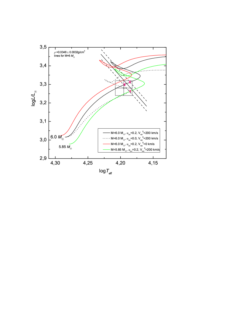
Figure 1: The error box from J2013 shows the position of $\mu$ Eri in the HR diagrams. The oblique straight lines correspond to the range of the mean density found in J2013 at $M={}$6 M_☉. The evolutionary tracks shown in this figure were calculated at metallicity $Z={}$0.015. Values of mass, overshooting parameter, $\alpha_{\rm ov}$, and the equatorial velocity, $V_{\rm rot}$, at the ZAMS are given in the legend. Selected models are shown with the crosses.

2.2 New three-band photometric data

New photometric measurements of $\mu$ Eri, consisting of differential time-series photoelectric data in the Strömgren $uvy$ filters, were acquired in the season 2012-2013. The star was measured alternatingly with the $\beta$ Cephei star $\nu$ Eri and $\xi$ Eri, using the 0.75-m Automatic Photoelectric Telescope (APT) T6 at Fairborn Observatory in Arizona.

The data were reduced in a standard way for photoelectric time-series photometry. First, the measurements were corrected for coincidence losses. Then, sky background was subtracted and nightly extinction coefficients, determined from the measurements of $\xi$ Eri via the Bouguer method (fitting a straight line to a magnitude vs air-mass plot). At a given air mass, the same extinction correction was applied to each star. Finally, differential magnitudes were computed by interpolation, and the timings were converted to Heliocentric Julian Date. We ended up with some 1120 data points for $\mu$ Eri obtained in 91 nights, for a total of 365 hr of measurement with a time span of 187.8 d.

We note that Handler et al. (2004) and J2005 reported low-amplitude variability of $\xi$ Eri, probably due to a $\delta$ Scuti-type pulsation. As such variations could not be detected in the present data set, we treated $\xi$ Eri as a constant comparison star. The time series obtained for $\nu$ Eri will be discussed elsewhere; we concentrate on $\mu$ Eri in what follows.

2.3 Significant frequency peaks

For the frequency analysis, we used the 2002-2003 and 2003-2004 MSC $v$-filter data, the 2009 MOST data, and the 2012-2013 APT $v$-filter data. In all cases, observations between the first and the last contact of the eclipses, i.e. those falling within $\pm\,$0.03 orbital phase away from the mid-eclipse epochs computed from the ephemeris provided by J2013, were omitted. In order to eliminate the short-period variations of unknown origin in the MOST data, the data were averaged in adjacent segments of about 0.044 d duration (see the Appendix in J2013). For consistency’s sake, the ground-based data were treated likewise. Mean light-levels were subtracted from the ground-based data; the MOST data were de-trended (J2013 Section 3.1). After these modifications, the data included 1354 data-points (845 2002-2003 and 2003-2004 MSC, 204 MOST, and 305 2012 APT), spanning 3850 d; the frequency resolution was therefore equal to 0.00026 c/d. The analysis consisted of computing an amplitude spectrum, identifying the highest peak, pre-whitening etc. The results were the following (in the parentheses, the signal-to-noise ratio is given): 0.6158 c/d (14.4), 0.7009 c/d (8.9), 1.2056 c/d (6.6), 0.6589 c/d (5.4), 0.5681 c/d (5.1), 0.8129 c/d (4.4), 0.4046 c/d (4.1), and 1.1810 c/d (3.8). The noise was computed as a straight mean of the amplitudes in the frequency range 0.3 to 1.3 c/d, obtained from the amplitude spectrum of the data pre-whitened with the above eight frequencies.

The first six frequencies are very nearly equal to the frequencies $f^{\prime}_{1}$, $f^{\prime}_{2}$, $f^{\prime}_{4}$, $f^{\prime}_{5}$, $f^{\prime}_{6}$, and $f^{\prime}_{3}$ of table 7 of J2005. In all cases the signal to noise is greater than 4, so that they all fulfill the popular criterion of significance of Breger et al. (1993). Additional arguments in favour of the significance of $f^{\prime}_{5}$, $f^{\prime}_{6}$, and $f^{\prime}_{3}$ are the following (1) the frequency quadruplet $f^{\prime}_{6}$, $f^{\prime}_{1}$, $f^{\prime}_{5}$, $f^{\prime}_{2}$, although not resolved by the MOST data, is necessary to account for the MOST doublet $f_{1}$, $f_{2}$ (see J2013, Section 9.1) and (2) $f^{\prime}_{3}$ is close to the highly significant MOST frequency $f_{7}$ (the difference $f_{7}-f^{\prime}_{3}$ is equal to one fourth of the frequency resolution of the MOST data). Thus, we retained the six frequencies, leaving the remaining ones for future verification by means of satellite data with sufficient frequency resolution. Using the frequencies $f^{\prime}_{i}$ ($i={}$1,..,6) as starting values in a nonlinear least-squares fit to the ground-based not-averaged $v$ data we obtained: $\nu_{1}={}$0.6157633$\,\pm\,$0.0000021, $\nu_{2}={}$0.7008807$\,\pm\,$0.0000044, $\nu_{4}={}$1.2055398$\,\pm\,$0.0000046, $\nu_{5}={}$0.6588788$\,\pm\,$ 0.0000058, $\nu_{3}={}$0.812899$\,\pm\,$0.000008 and $\nu_{6}={}$0.568107$\,\pm\,$0.000007 c/d. Finally, for $\nu_{i}$ ($i={}$1,..,6), the $uvy$ amplitudes and phases were computed by means of linear least-squares using the ground-based data. The results are listed in Table 2. The standard deviations of the amplitudes and phases (given in parentheses without the leading zeroes) are the formal standard deviations of the least-squares solutions multiplied by two. In this, we follow Handler et al. (2000) and J2005 who—while dealing with time-series observations similar to the present ones—showed that the formal standard deviations were underestimated by a factor of about two.

Table 2: Amplitudes and phases in the $uvy$ Strömgren passbands for six frequency peaks found in the light curve of $\mu$ Eri. The function $\sum_{i=1}^{6}A_{i}\cos(2\pi\nu_{i}(t-t_{0})-\varphi_{i})$ was fitted with the zero-epoch, $t_{0}$, equal to HJD 245 4450.

	$A$ [mag]	$\varphi$ [rad]
$\nu_{1}={}$0.6157633(21) c/d, $S/N={}$14.4
$u$	0.00974(15)	4.2832(148)
$v$	0.00626(11)	4.3011(169)
$y$	0.00536(10)	4.3342(177)
$\nu_{2}={}$0.7008807(44) c/d, $S/N={}$8.9
$u$	0.00467(14)	3.9164(308)
$v$	0.00292(11)	4.0975(361)
$y$	0.00238(10)	4.0058(s397)
$\nu_{3}={}$0.812899(8) c/d, $S/N={}$4.4
$u$	0.00224(14)	1.6037(647)
$v$	0.00168(11)	1.7779(634)
$y$	0.00115(10)	2.0308(820)
$\nu_{4}={}$1.2055398(46) c/d, $S/N={}$6.6
$u$	0.00327(15)	1.7280(436)
$v$	0.00275(11)	1.9930(384)
$y$	0.00251(10)	2.0943(378)
$\nu_{5}={}$0.6588788(58) c/d, $S/N={}$5.4
$u$	0.00375(14)	1.4119(389)
$v$	0.00235(11)	1.4735(460)
$y$	0.00234(9)	1.4820(416)
$\nu_{6}={}$0.568107(7) c/d, $S/N={}$5.1
$u$	0.00264(14)	1.8346(562)
$v$	0.00183(11)	1.9181(599)
$y$	0.00176(9)	1.8882(549)

The frequency $\nu_{3}$ is an exact multiple of the orbital frequency, i.e., $\nu_{3}=6/P_{\rm orb}$. Given the significant eccentricity of the binary system, this frequency may arise as a tidal effect. As we shall see in Section 5, assuming different origins of this frequency requires only a small modification of our search for mode identification and it is inconsequential for the results.

In Fig. 2, we show the amplitude ratios in two colours plotted against the corresponding phase differences. Such diagrams are often used for revealing the mode degree, $\ell$. If the effects of rotation are large, a direct inference is not possible. Nonetheless, the diagrams are still useful for presenting data and their errors. Two pairs of passbands were considered: $(u,v)$ and $(u,y)$. Let us note the large phase differences for peaks $\nu_{3}$ and $\nu_{4}$.

Typically for SPB stars the phase difference in any two passbands is close to zero, which is expected if the temperature variations dominate. Ignoring the effects of rotation, Townsend (2002) and De Cat et al. (2004) found the $\ell={}$1 identification for most modes in SPB stars known at that time. However, most of these SPB stars are slower rotators than $\mu$ Eri as shown by De Cat et al. (2005). Let us remind the reader that a dipole mode does not cause variations of the star’s shape.

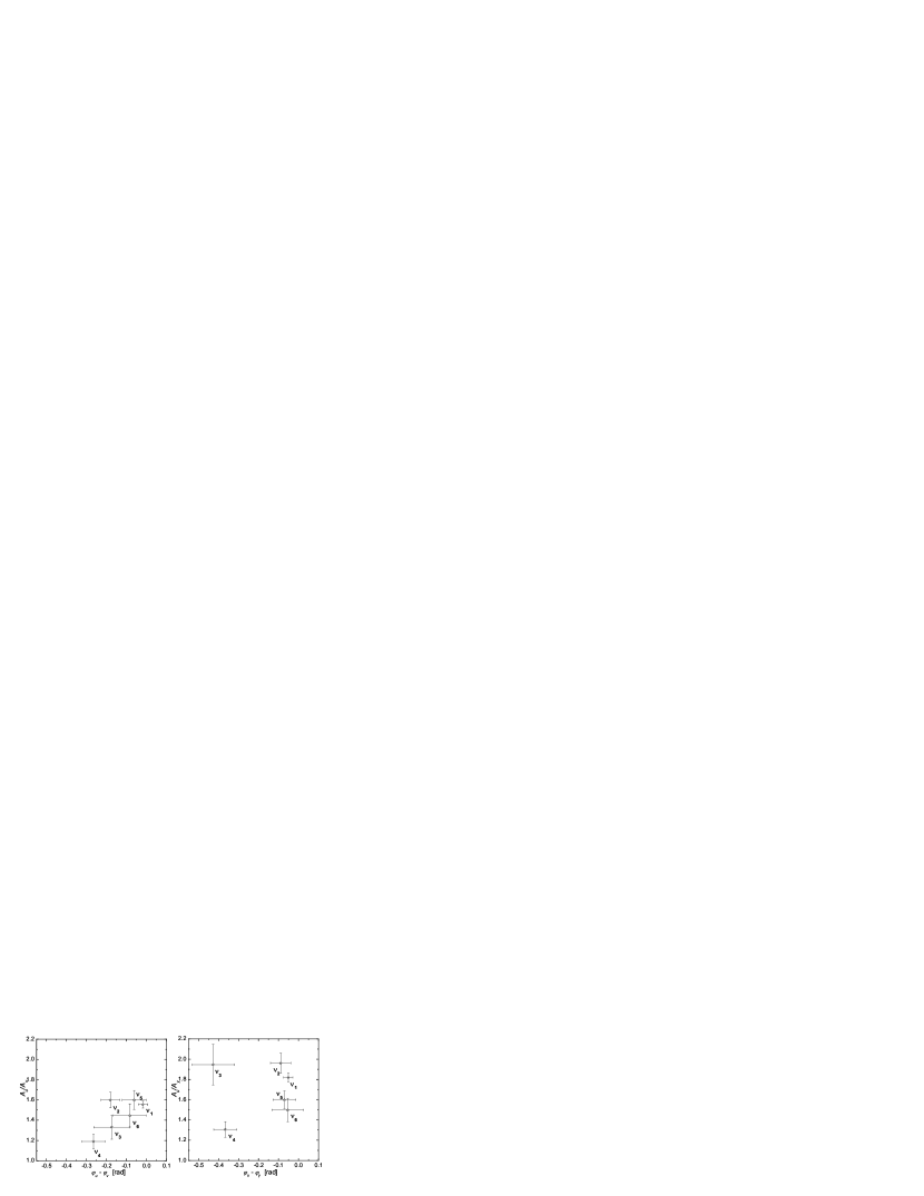
Figure 2: Amplitude ratios and phase differences for significant frequency peaks of $\mu$ Eri in the photometric diagnostic diagrams involving two pairs of the Strömgren passbands: $(u,v)$ and $(u,y)$, showed in the left and right panel, respectively.

3 Unstable modes

Looking for possible identifications of the frequency peaks, we focus on unstable modes. In Section 5, we will abandon this requirement for the frequency $\nu_{3}$ which may be resonantly excited by the companion to the pulsator in the $\mu$ Eri binary system.

At these low frequencies, we must consider not only gravity modes but also mixed-Rossby modes, which appear at high rotation rate. They are retrograde with $m=-\ell$. In the present paper we will refer to them as the r-mode and identify them through the $m$ value alone. Savonije (2005) and Townsend (2005) showed that they may become unstable. In our stability analysis we use a nonadiabatic generalisation of the traditional approximation ((Dziembowski, Daszyńska-Daszkiewicz & Pamyatnykh, 2007)). The only modification of the equations for nonadiabatic oscillations in nonrotating stars (in the Cowling approximation) is the replacement of $\ell(\ell+1)$ with $\lambda$, which is the eigenvalue of the Laplace tidal equation (see e.g. Bildsten, Ushomirsky & Cutler, 1996; Lee & Saio, 1997; Townsend, 2003a). At finite rotation rate, we have $\lambda=\lambda(\ell,m,s)$, where $s=2\nu_{\rm rot}/\nu_{*}$ (the spin parameter) and $\nu_{*}$ is the eigenmode frequency in the corotating system. For all g-modes $\lambda(\ell,m,0)=\ell(\ell+1)$. For the prograde sectorial modes ($m=\ell$), $\lambda$ slowly decreases with $s$, asymptotically tending to $m^{2}$, whereas for other modes it sharply increases (e.g. Townsend, 2003a), which is also true for the r-modes once they appear at $s=|m|+1$. We put the azimuthal and temporal dependence in the form ${\rm exp}[{\rm i}(m\varphi-2\pi\nu_{*}t)]$, which implies $m>0$ for prograde modes and $m<0$ for retrograde modes. Thus, the frequency in the inertial system is given by $\nu=|\nu_{*}+m\nu_{\rm rot}|$.

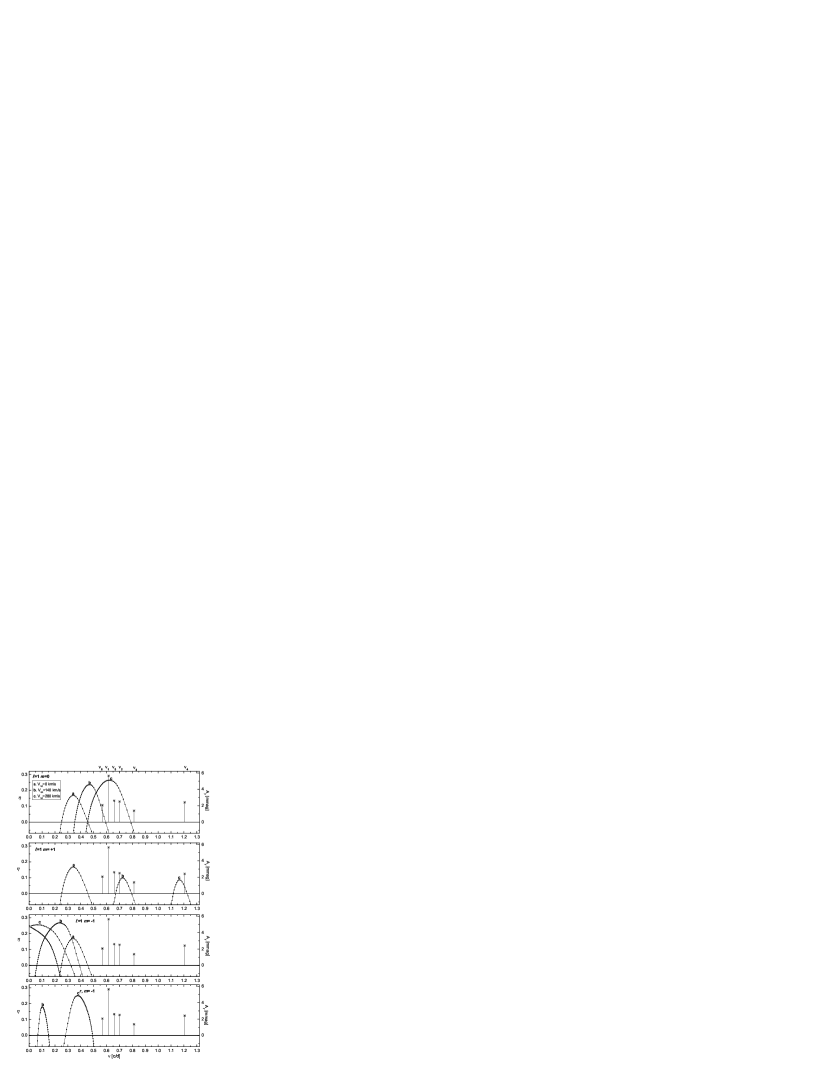
Figure 3: The normalized instability parameter $\eta$ as a function of the frequency in the inertial system for g-modes at $\ell={}$1 and r-modes at $m={}-$1 in Model 1 (see Table 1). Three values of a rotational velocity were considered: 0, 140 and 280 km/s, marked as a, b, c, respectively. Amplitudes of the observed peaks in the $y$ Strömgren passband are given on the right axis.

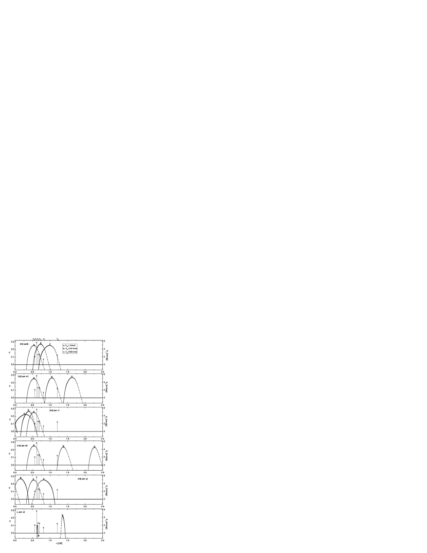
Figure 4: The same as Fig. 3 but for g-modes at $\ell={}$2 and r-modes at $m={}-$2.

According to Lee (2010), the number of unstable retrograde g-modes is much smaller if the truncated Legendre expansion is used instead of the traditional approximation. Thus, perhaps some of the modes that we allow should be excluded. On the other hand, Savonije (2007) with his 2D models largely confirmed results of Dziembowski et al. (2007) regarding instability of the retrograde modes obtained with the approximation adopted in the present work.

Following Stellingwerf (1978), we measure mode instability with the normalized growth rate

$$\eta=\frac{W}{\int_{0}^{R}\left|\frac{dW}{dr}\right|dr}$$

where $W$ is the usual work integral over the pulsational cycle. From this definition, it follows that $\eta$ varies in the range $[-1,+1]$ and it is positive ($\eta>0$) for unstable modes, that we regard as possible candidates for interpretation of the oscillation spectrum of $\mu$ Eri.

In Fig. 3, we show the values of $\eta$ plotted against frequency in the observer’s system for gravity modes with $\ell={}$1 and r-modes with $m={}-$1 in Model 1. In each panel we show also frequencies and the $y$ Strömgren amplitudes of the six significant peaks detected in $\mu$ Eri. The mode frequencies were calculated for rotation rates 0, 140 and 280 km/s. Let us remind that in this model the mean effect of centrifugal force is evaluated at $V_{\rm rot}\approx{}$170 km/s. However, our intention here was to show only the effects of rotation induced by the Coriolis force and the Doppler effect. Consequences of changes in the model caused by the changes of centrifugal force at the same $T_{\rm eff}$ are much smaller. Fig. 4 shows the same but for the $\ell={}$2 g-modes and the $m={}-$2 r-mode.

The top panels of Figs. 3 and 4 show a pure effect of the Coriolis force ($m={}$0). The frequencies of the unstable modes increase with rotation rate. In the adopted approximation, the effect is equivalent to a continuous increase of $\ell$ in nonrotating stars. Notice that the sequence ,,b” in Fig. 4 is quite similar to the sequence ,,c” in Fig. 3. Both cover the range of the four lowest frequency peaks. However, these peaks cannot be associated with consecutive radial orders, as thought by J2005, because the separations between them are too large. If rotation is fast enough, the $\ell={}$1, $m={}$0 and $\ell={}$2, $m={}$0 identifications are also possible for $\nu_{3}$. The latter identification is also acceptable for $\nu_{4}$.

The plots for the $\ell=m$ modes reveal mainly the effect of the Doppler frequency shift because changes of $\lambda$ for sectoral prograde modes are small. Since 130 km/s is adopted as the minimum equatorial velocity, the $m=\ell={}$1 identification could be the only one for the four highest frequency peaks and the $m=\ell={}$2 identification, the only one for the $\nu_{4}$ peak.

None of the peaks may be associated with the $\ell={}$1, $m={}-$1 mode nor the $m={}-$1, r-mode. The $\ell={}$2, $m={}$1 identification is possible for $\nu_{4}$ but at a lower rotation rate than the $\ell={}$2, $m={}$0 identifications. The $\ell={}$2, $m=-{}$1 mode may be responsible for one or two peaks of lowest frequency. The $\ell={}$2, $m={}-$2 identification is possible for all the peaks except for $\nu_{4}$ if rotation is fast enough. The instability ranges for the r-modes are narrower than for g-modes. Yet, at $m={}-$2 the r-modes may account for all observed peaks except $\nu_{6}$.

Instability of g-modes continues well beyond $\ell={}$2. In Model 1 it goes up to $\ell={}$17 and extends for many radial orders. At the zero rotation rate there are altogether about $1.5\times 10^{4}$ unstable modes. At $V_{\rm rot}={}$280 km/s, the number of unstable modes is about 30 percent lower. The effect of increasing rotation rate on the r-mode instability is opposite but the number of unstable r-modes is always much smaller than that of g-modes.

The large number of unstable modes follows, in part, from their high radial orders, $n$, which range from 25 to 101 and imply small frequency separations between consecutive modes, and, in part, from the favorable shape of the eigenfunctions (relatively large amplitudes in the driving zone) in wide frequency ranges.

Figure 5: Instability domain in the $(\lambda^{1/2},\nu_{*})$ plane for Model 1. Pairs of symbols at the same values of $\lambda=\ell(\ell+1)$ determine the frequency range of unstable modes at $\ell={}$1 to 17. These ranges were calculated with the standard nonadiabatic pulsation code ignoring effects of the Coriolis force. The instability domain is the same with the traditional approximation but then $\lambda$ depends on $\nu_{*}$. In the three panels, examples of the $\lambda^{1/2}(\nu_{*})$ dependence for retrograde, zonal, and prograde modes are shown. The solid and dashed lines correspond to $V_{\rm rot}={}$280 and 140 km/s, respectively.

The mode order and the amplitude behavior in the stellar interior is determined by the value of $\lambda^{1/2}/\nu_{*}$. The extent of the instability range in $\nu_{*}$ follows from a requirement of a match between the pulsation period and the thermal time scale in the driving zone. This sets the upper limit on $\lambda$, which at the specified $\ell$ and $m$ depends on $V_{\rm rot}$. However, as one may see in Fig. 5, the dependence is weak, except for the zonal modes. In the two upper panels of Fig. 5, we may see that at a specified frequency, $\lambda$ increases with the rotation rate, causing some modes to move out of the instability domain. Only at $\ell=m$ the value of $\lambda$ slightly decreases with $V_{\rm rot}$. For other prograde modes, like for the modes shown in the two upper panels, it does increase.

The instability ranges are sensitive to the effective temperature. With the lower $T_{\rm eff}$ and lower $L/M$ ratio, the ranges move to higher frequencies. Thus, the unstable $\nu_{*}$- ranges in Model 2 are shifted towards the higher frequencies relative to those in Model 1 and to the lower ones relative to those in Model 3.

4 Visibility of the pulsational modes

Looking for possible mode identifications, we have to take into account mode visibility. Large effects of rotation on the slow modes visibility arising at moderate rate were first studied by Townsend (2003b) with the traditional approximation. This approximation was also adopted in D07a and is used in this paper. Recently, a treatment of the visibility based on 2D stellar models was developed by Reese et al. (2012) and Savonije (2013) with all dynamical effects of fast rotation taken into account. However, utility of the treatment presented in the first paper is limited due to the adopted adiabatic relation between pressure and temperature changes.

In the traditional approximation, the latitudinal dependence of the the radial displacement is described by the Hough functions, $\Theta_{\ell}^{m}(\theta)$, which become the associated Legendre functions, $P_{\ell}^{m}(\theta)$, in the limit of zero-rotation rate. At finite rotation, mode visibility depends not only on $\ell$, $m$, but also on the aspect angle, $i$, and the spin parameter, $s$. Our inferred values of $s$ for the six peaks listed in Table 2 are between 0.7 and 1.6.

Most of the unstable modes have frequencies much higher than those detected in $\mu$ Eri. Still, if the instability is the only constraint on the mode geometry, the number of potential identifications to consider is quite large. At $V_{\rm rot}={}$140 km/s, there are about 60 possible identifications for each peak with the angular degrees ranging up to $\ell={}$17. At $V_{\rm rot}={}$280 km/s, the number of possible identifications is reduced to about 20 and the maximum $\ell$ is 14. At high values of $\ell$, only retrograde modes of moderate $m$ fall into the observed range and, as we noted in the previous section, they actually may be stable. In any case, the number of possible identifications remains large if the visibility argument is not taken into account.

At slow rotation, the decline of the disc averaging factor, $b_{\ell}$ (see e.g. Daszyńska-Daszkiewicz et al., 2002), is often used to justify limiting the search for identifications to modes with $\ell\leq 2$. Rotation complicates the matter of mode visibility considerably. The counterpart of this factor within the traditional approximation is given by

$$b_{\ell,m}^{x}=\int_{0}^{1}h^{x}(\mu)\mu\Theta_{\ell}^{m}(\theta)d\mu,$$

where $\mu=\cos\theta$, $x$ denotes the photometric passband, $h^{x}(\mu)$ is the limb-darkening law and $\Theta_{\ell}^{m}(\theta)$ are the Hough functions. Now $b_{\ell,m}$ depends additionally on $m$ and the spin parameter, $s$.

Figure 6: The values of the disc averaging factor, $b_{\ell,m}^{V}$, in the Geneva $V$ filter as a function of the mode degree, $\ell$, for the three values of the spin parameter, $s={}$0.0,1.0,2.0 from top to bottom. The $m$ values at the points corresponding to extreme values of $b_{\ell,m}^{V}$ at each $\ell$ are given.

In Fig. 6, we show the absolute values of $b_{\ell,m}$ in the Geneva $V$ passband as a function of $\ell$ for three values of $s$. The top panel is for $s={}$0, i.e., for the zero-rotation limit. Note the one order of magnitude drop between $\ell={}$2 and 3. This drop is significantly reduced to about a factor of 2 at $s={}$1 and $m={}-$1. Modes with $m={}-$1 at higher values of $\ell$ also do not suffer such reduced visibility. The cause is a significant contribution from the $P_{\ell}^{-1}$ component in the expansion of $\Theta_{\ell}^{m}$ in a series of the associated Legendre functions. The situation is quite different at $s={}$2. In particular, modes with different azimuthal orders become best visible. The non-monotonic character of the $b_{\ell,m}(s)$ dependence arises from changing the contributions from the low- to high-degree $P_{\ell}^{m}$ components in $\Theta_{\ell}^{m}$. Thus, the effects of rotation complicate the matter of mode visibility. In the present work, the systematic search for possible mode identifications for $\mu$ Eri was stopped at $\ell={}$6.

5 Modes excited in $\mn@boldsymbol{\mu}$ Eri and its rotation rate

The source of observational information on the angular numbers of the excited modes are the amplitudes and phases in various photometric passbands and in the radial velocity. Diagrams showing amplitude ratios vs phase differences, such as those shown in Fig. 2, are often used for this goal. If the effects of rotation are negligible, these parameters are independent of the inclination angle and the azimuthal order, $m$, and, in favorable conditions, the $\ell$ degree may be inferred from the peak location in the amplitude ratio vs phase difference diagnostic diagram.

Mode locations in the diagnostic diagrams at non-zero rotation rate depend on the inclination angle, azimuthal order and rotational velocity, $V_{\rm rot}$. Even at low rotation rate, the coupling of modes with the same $m$ and $\ell$ differing by two – caused by the centrifugal distortion – may result in large shifts in the diagnostic diagrams (Daszyńska-Daszkiewicz et al., 2002). This effect is ignored in the traditional approximation adopted in the present work but it is unlikely to be important for the considered modes.

Here we follow the approach outlined in D07a.

5.1 The mode discriminant

The basis of our method of mode identification is equation (20) in D07a. Here, we write it in a more compact form,

$${\cal A}_{k}=\varepsilon{\cal F}_{k}(i).$$

This equation connects the complex amplitude of the peak,

$${\cal A}_{k}\equiv A_{k}\exp(\rm i\varphi_{k}),$$

in the $k$-band to the complex amplitude of the associated mode, $\varepsilon$. This amplitude is related to the relative surface radius variation through the expression

$${\delta R\over R}=\varepsilon\Theta_{\ell}^{m}(\theta)\exp[{\rm i}(m\phi-2\pi\nu t)].$$

The ${\cal F}_{k}$-coefficients split into two terms,

$${\cal F}_{k}(i)={\cal D}^{k}(i)f+{\cal E}^{k}(i).$$

The first term arises from the temperature perturbation and the second from the displacement of the surface element. The $f$-factor describing the response of the flux to the radius change is a complex quantity which may be obtained from nonadiabatic calculations together with the instability parameter $\eta$ for a specified stellar model. The expressions for ${\cal D}^{k}$ and ${\cal E}^{k}$, which come from the integration of local contributions over the stellar disc with the limb darkening factor and its perturbation taken into account, were given in D07a. The expressions are very long and need not be repeated here.

Data on stellar surface parameters and atmospheric models are needed to convert changes in radius and effective temperature into changes in monochromatic fluxes. We need also information about the rotation rate and the inclination angle. Rotation affects the stellar model but also, which is more important, the values of the terms ${\cal D}^{k}$ and ${\cal E}^{k}$ through its influence on the $\Theta_{\ell}^{m}(\theta)$ dependence.

Given ${\cal F}_{k}$ and the data from the three passbands, we have three complex linear equations for $\varepsilon$, implying four degrees of freedom. Thus we may use

$$\chi^{2}=\frac{1}{4}\sum_{k=1}^{3}w_{k}|\varepsilon{\cal F}_{k}(i)-{\cal A}_{k}|^{2},$$

as the mode and the inclination discriminant, where $w_{k}$ are the statistical weights defined by the observational errors

$$w_{k}=|\sigma_{k}|^{-2}.$$

For a given pulsation mode and specified stellar parameters, we search for the best value of $\varepsilon$ to fit photometric amplitudes and phases in all passbands simultaneously

$$\frac{\partial\chi^{2}}{\partial\varepsilon}=0.$$

Thus the $\chi^{2}$-minimization yields the following expression for the mode’s complex amplitude

$$\varepsilon=\frac{\sum_{k=1}^{3}w_{k}{\cal A}_{k}{\cal F}_{k}^{*}}{\sum_{k=1}^{3}w_{k}|{\cal F}_{k}|^{2}},$$

where ${\cal F}_{k}^{*}$ is the complex conjugate.

Mode amplitudes, $\varepsilon$, are observational characteristics that cannot be compared with calculations because nonlinear modeling of nonradial stellar oscillations is far ahead of us. Nonetheless, the values of $|\varepsilon|$ deduced from data are of interest as a hint towards understanding the mechanism of amplitude limitation. In the present work, the values of $\varepsilon$ were used to constrain mode identification.

Even if $\chi^{2}$ is small, we cannot accept identifications if they imply too large values of $\varepsilon$ because all known SPB stars are low amplitude pulsators. De Cat (2007), who compiled data on nearly two hundred (including candidates) SPB stars, found no object with an amplitude above $A_{V}=0.03$ mag. We may use this information to assess the upper limit of $\varepsilon$ (denoted $\varepsilon_{\rm max}$), assuming, which seems justified, that the peaks with the highest amplitudes are due to modes with the highest values of $\varepsilon$ and the highest values of ${\cal F}_{k}$. For given stellar model, the highest values of $|{\cal F}_{k}|$ occur at $\ell=1,m=0$ and $i=0^{\circ}$. Considering values of $|f|$ (see Eq. 3) for unstable dipolar modes in stellar models corresponding to the highest amplitude SPB star HD181558 ($A_{V}=0.028$ mag) (de Cat, 2007), we found the average value $\overline{|{\cal F}_{V}|}\approx$3 mag for $i=0^{\circ}$. Therefore, we decided to reject the identification if

$$|\varepsilon|\geq\varepsilon_{\rm max}=0.01.$$

An additional constraint on $\varepsilon$ follows from the limit of the radial velocity amplitude of 2 km/s found by J2013. Having the mode identification and $\varepsilon$ from photometry, we may calculate the radial velocity amplitude, $A_{V_{\rm rad}}^{\rm cal}$, and confront it it with the observational bound. Equation (18) of D07a yields

$$A_{V_{\rm rad}}^{\rm cal}=2\pi R\nu|{\varepsilon\cal C}_{\rm puls}+{\cal C}_{\rm rot}|,$$

where ${\cal C}_{\rm puls}$ and ${\cal C}_{\rm rot}$ describe direct contributions from pulsation and from pulsational modulation of rotation, respectively. The complicated expressions for these two coefficients are not required here. It suffices to know that they are fully determined by the atmospheric parameters of the star and the Hough functions of the mode.

With $\varepsilon$ given by equation (5), we get from equation (4) a more explicit expression for our mode discriminant,

$$\chi^{2}=\frac{1}{4}\left(\sum_{k=1}^{3}w_{k}|{\cal A}_{k}|^{2}-\frac{\sum_{k=1}^{3}w_{k}|{\cal A}_{k}{\cal F}_{k}^{*}|^{2}}{\sum_{k=1}^{3}w_{k}|{\cal F}_{k}|^{2}}\right).$$

Here, unlike the case of the most often used mode discriminants, the data from the three passbands are treated equally. We see this as the main advantage of our approach to mode identification.

5.2 A constraint on the rotation rate

In the way described above, we may find acceptable mode identification(s) for individual peaks at a specified confidence level, stellar model and the inclination of the rotation axis. The range of parameters where a particular identification applies is, in general, different for different peaks. The requirement of consistency sets constrains on possible identifications and on admissible ranges of stellar parameters.

The most important are the constraints on rotation. Firstly, because from spectroscopy we may assess only the value of $V_{\rm rot}\sin i$. Secondly, because some identifications are acceptable only in very narrow ranges of the inclination.

5.3 Results

Figure 7: Fitting of eigenmodes of Model 1 (see Table 1) to complex amplitudes for the six significant frequency peaks in $\mu$ Eri. The dots show minimum values of $\chi^{2}$ calculated with equation (8). The numbers give the degrees, $\ell$, and azimuthal orders, $m$, of the modes. The range of $V_{\rm rot}$ corresponds to a $[90^{\circ},28^{\circ}]$ range of the inclination angle.

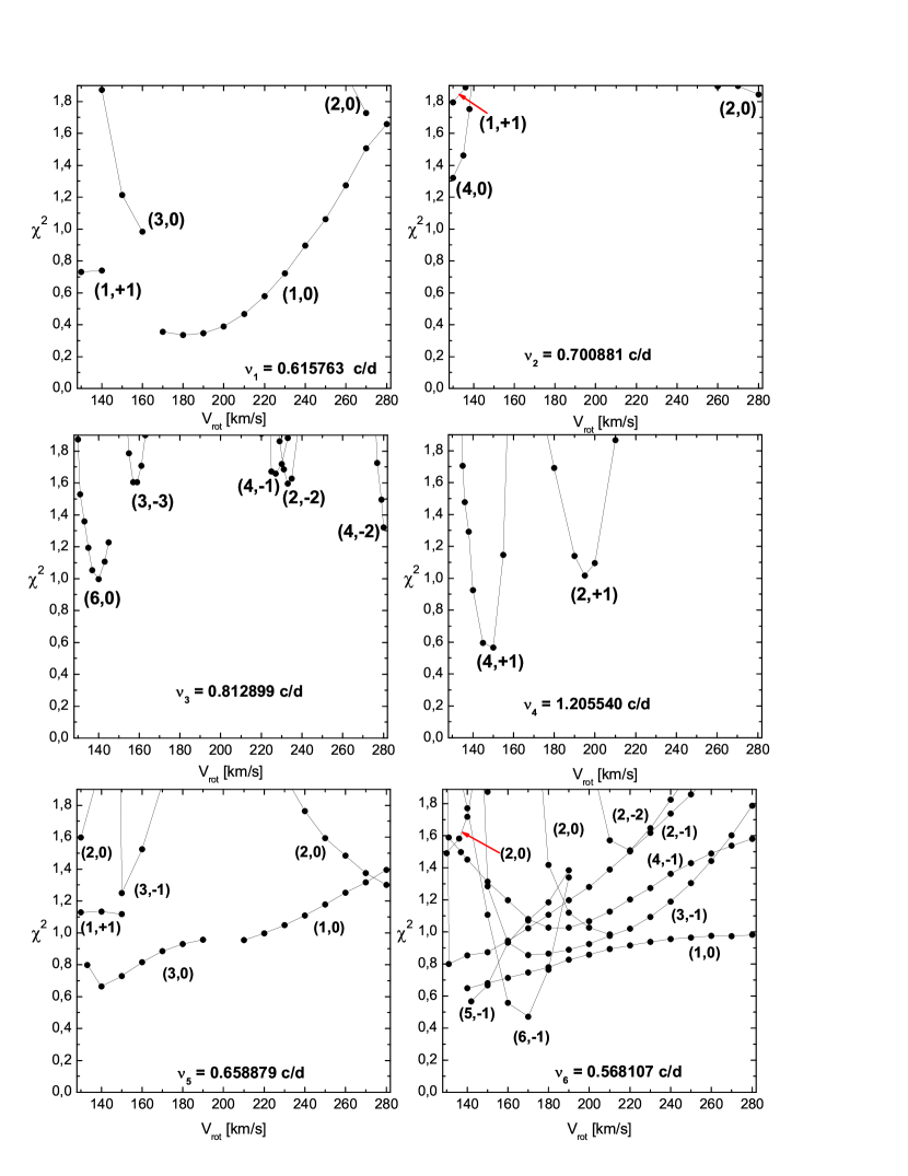
Figure 8: The same as Fig.  7 but for Model 2.

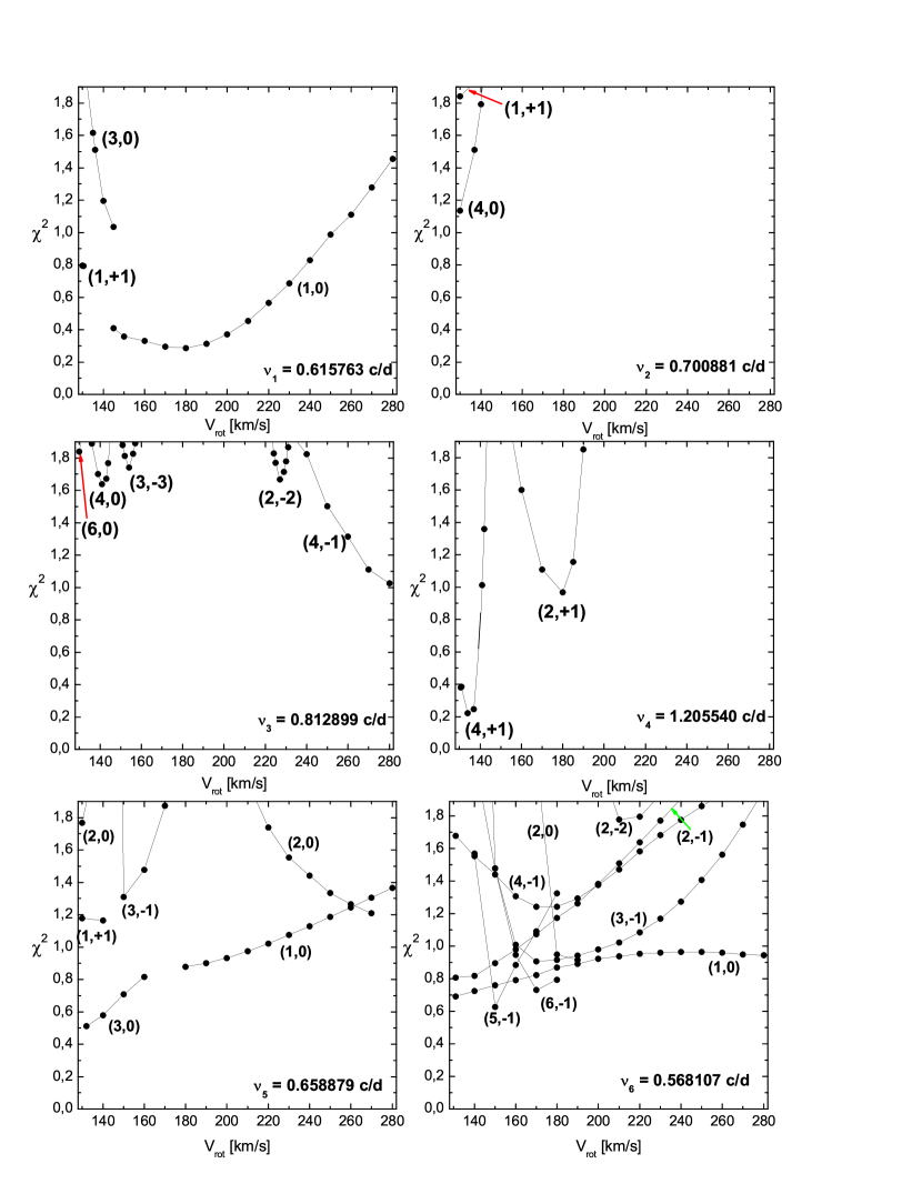
Figure 9: The same as Fig.  7 but for Model 3.

We adopted Kurucz’s (2004) tables based on his stellar atmosphere models for calculations of ${\cal D}^{k}$, ${\cal E}^{k}$, ${\cal C}_{\rm puls}$ and ${\cal C}_{\rm rot}$ needed in equations (3) and (7). The limb darkening coefficient and its changes were calculated with the help of Claret’s (2000) expressions.

Both the rotation rate and inclination of the rotation axis, have significant impact on mode identification. In order to limit the number of adjustable parameters, we fixed $V_{\rm rot}\sin i$ at the spectroscopic value of 130 km/s. We did not consider $\sin i<0.46$ implying $V_{\rm rot}>280$ km/s because it would be too high for our simplified treatment. An 80 percent confidence level has been adopted for rejection of a mode identification. This corresponds to a $\chi^{2}={}$1.5 upper limit for the acceptable identifications.

The set of modes considered for the six frequency peaks in $\mu$ Eri included all unstable g-modes with the $\ell$ degrees up to 6 and r-modes with the $|m|$ orders up to 3. Unstable r-modes with $|m|>3$ have frequencies much higher than the highest frequencies observed in $\mu$ Eri. We will discuss the consequences of the bound on radial velocity amplitude later on but in our initial mode identification we will take into account only the conditions

$$\chi^{2}\leq 1.5,\qquad\varepsilon\leq 0.01,\qquad\mbox{and}\quad\eta\geq-0.05.$$

The last condition is a somewhat liberalized (in view of uncertainties) instability condition.

As we mentioned in Section 2, the frequency $\nu_{3}$ is equal to $6/P_{\rm orb}$. Therefore, for identification of $(\ell,m)$ of $\nu_{3}$ we have to allow also stable modes, i.e., not excited by the $\kappa$ mechanism. However, to account for the amplitudes, $\varepsilon$, listed in Tables 4 to 6, a close proximity of the stellar eigenfrequency to $6/P_{\rm orb}$ is needed because for the equilibrium (non-resonant) tide the corresponding amplitudes are by orders of magnitude lower.

The values of $\chi^{2}$ for the six peaks plotted against the rotational velocity are depicted in Figs. 7, 8, and 9. They were obtained with the use of Models 1, 2, and 3, respectively.

As we may see in Fig. 7, there are two possible identifications for the $\nu_{1}$ peak. The $\ell={}$1, $m={}$0 identification is acceptable in the whole range of $V_{\rm rot}$ we consider, beginning from about 140 km/s. At lower $V_{\rm rot}$, this peak is outside the instability range for the $\ell={}$1, $m={}$0 modes (see Fig. 3). Below, but only down to 138 km/s, the (3,0) identification becomes acceptable and, in fact, the only acceptable one with the constraint on rotation set by the unique (4,0) identification for the $\nu_{2}$ peak. In the very narrow $V_{\rm rot}$ range allowed by the identification of the $\nu_{2}$ peak, the unique possibilities are: (4,0) for the $\nu_{3}$ peak and (4,+1) for the $\nu_{4}$ peak. The latter identification imposes an upper limit on the equatorial velocity of 138.2 km/s and the allowed range of $V_{\rm rot}$ reduces to a small fraction of 1 km/s. Still, for the remaining two peaks we have a number of options. All acceptable identifications for the six peaks together with the associated values of $|\varepsilon|$ and $A_{V_{\rm rad}}^{\rm cal}$ are listed in Table 3.

Table 3: Modes in Model 1 that may be associated with the six frequency peaks in $\mu$ Eri with the constraints given in equation 9. The amplitudes $|\varepsilon|$ and $A_{V_{\rm rad}}^{\rm cal}$ were calculated with the use of equations 5 and 7, respectively. The equatorial velocity $V_{\rm rot}\approx{}$138 km/s, which corresponds to $i\approx{}$70^∘, results from fitting the frequencies $\nu_{1}$ and $\nu_{4}$. The corresponding value of the rotational frequency is $\nu_{\rm rot}=0.44$ c/d.

frequency [c/d]	$(\ell,m)$	$|\varepsilon|$	$A_{V_{\rm rad}}^{\rm cal}$ [km/s]
$\nu_{1}={}$0.615763	$(3,0)$	0.0055	6.0
$\nu_{2}={}$0.700881	$(4,0)$	0.0024	0.3
$\nu_{3}={}$0.812899	$(4,0)$	0.0022	0.4
$\nu_{4}={}$1.205540	$(4,+1)$	0.0032	2.1
$\nu_{5}={}$0.658879	$(1,+1)$	0.0003	1.3
	$(3,0)$	0.0030	2.2
$\nu_{6}={}$0.568107	$(1,0)$	0.0017	1.5
	$(2,-1)$	0.0015	0.7
	$(4,-1)$	0.0018	0.6

The problem with the mode identifications presented in Table 3 is caused by the high radial velocity amplitudes that are implied for some of the peaks. In particular, for the dominant $\nu_{1}$ peak, the calculated amplitude exceeds by a factor of 3 the observed limit of 2 km/s. A reliable comparison requires that the spectroscopic value is derived from the changes in the first moments of spectral lines and that spectroscopic and photometric data are roughly contemporaneous. These conditions are not satisfied in our case.

It is important to check how the mode identification depends on the choice of the reference model. What matters is not only the change in the instability ranges, discussed already in Section 4, but also the modification in mode visibility. The $f$-factor in equation (3) depends on $T_{\rm eff}$ and $L$. Also other terms in this expression would be somewhat modified by changes of $\lambda$ at fixed $V_{\rm rot}$ and $\nu_{*}$.

Comparing Figs. 8 and 9 with Fig. 7 we first note similarities. For instance, always the (1,0) identification is valid for the $\nu_{1}$ peak over the wide range of $V_{\rm rot}$ and (4,0) is the only identification for the $\nu_{2}$ peak and only in a very narrow range. However, with the requirement of the same $V_{\rm rot}$ for all peaks, the acceptable ranges become very narrow and we get significant differences in mode assignment. The ranges are not much different, $V_{\rm rot}\approx{}$136 km/s with Model 2 and 137 km/s with Model 3. In Tables 4 and 5, we list the mode identifications and the corresponding amplitudes. Note, in particular, the differences for the $\nu_{1}$ peak, which was assigned to an $\ell={}$3, $m={}$0 mode in Model 1. It should be noted that for the dominant peak with all models the lowest value of $\chi^{2}$ was obtained for the (1,0) identification but outside the $V_{\rm rot}$ range allowed by the peaks $\nu_{2}$ and $\nu_{4}$.

With Model 3 we obtained almost the same identifications as with Model 1. Only one possible identification for the $\nu_{6}$ peak has been eliminated. The same identification for the $\nu_{1}$ peak leads to even higher $A_{V_{\rm rad}}^{\rm cal}$. With Model 3, the problem is the fit for the $\nu_{3}$ peak which requires rising $\chi^{2}$ by about 0.1 above the limit set by conditions (9).

With Model 2, we obtained for the $\nu_{1}$ peak the (1,+1) identification and $A_{V_{\rm rad}}^{\rm cal}={}$3.3 km/s, which is still above the spectroscopic limit but much less so than in the other models. In view of the uncertainty in the spectroscopic limit, the 65% excess for the $\nu_{1}$ peak cannot be regarded as large. It could be further reduced by considering cooler models, somewhat outside the error box shown in Fig. 1. The associated $\varepsilon$ is more than an order of magnitude lower than 0.01. For all the remaining peaks, except for one of two possible identifications of $\nu_{5}$, the calculated radial velocity is below the 2 km/s limit and $\varepsilon$ is at most 0.006.

Table 4: The same as in Table 3, but for Model 2. The equatorial velocity is $\approx{}$136 km/s, as fixed by fitting the $\nu_{2}$ and $\nu_{4}$ peaks. The corresponding value of the rotational frequency is $\nu_{\rm rot}=0.42$ c/d.

frequency [c/d]	$(\ell,m)$	$|\varepsilon|$	$A_{V_{\rm rad}}^{\rm cal}$ [km/s]
$\nu_{1}={}$0.615763	$(1,+1)$	0.0008	3.3
$\nu_{2}={}$0.700881	$(4,0)$	0.0031	0.6
$\nu_{3}={}$0.812899	$(6,0)$	0.0040	1.1
$\nu_{4}={}$1.205540	$(4,+1)$	0.0033	1.3
$\nu_{5}={}$0.658879	$(3,0)$	0.0056	2.1
	$(1,+1)$	0.0005	1.5
$\nu_{6}={}$0.568107	$(2,-1)$	0.0016	0.7
	$(4,-1)$	0.0019	0.5

Table 5: The same as in Table 3, but for Model 3. The rotation velocity is $\approx{}$137 km/s as fixed by fitting the $\nu_{1}$ and $\nu_{2}$ peaks. The corresponding value of the rotational frequency is $\nu_{\rm rot}=0.44$ c/d. In order to fit an $\ell={}$4, $m={}$0 mode to $\nu_{3}$, we had to increase $\chi^{2}$ by about 0.2 above the limit set in equation (9).

frequency [c/d]	$(\ell,m)$	$|\varepsilon|$	$A_{V_{\rm rad}}^{\rm cal}$ [km/s]
$\nu_{1}={}$0.615763	$(3,0)$	0.0066	6.4
$\nu_{2}={}$0.700881	$(4,0)$	0.0028	0.1
$\nu_{3}={}$0.812899	$(4,0)$	0.0024	0.6
$\nu_{4}={}$1.205540	$(4,+1)$	0.0037	2.2
$\nu_{5}={}$0.658879	$(3,0)$	0.0037	2.4
	$(1,+1)$	0.0003	1.3
$\nu_{6}={}$0.568107	$(1,0)$	0.0021	1.6
	$(2,-1)$	0.0016	0.7

The modes we associated with $\nu_{3}$ are, in fact, unstable but for the tidal excitation this is irrelevant. What matters is only that the driving or damping rate is much lower than the frequency. However, it is important to stress that we end up with the same identification of the $\nu_{3}$ peak considering only unstable modes. None of the $|\varepsilon|$ values listed in Tables 3 - 5 comes close to 0.01, which was set as the upper limit for acceptable identifications.

We cannot exclude very different identifications if the equatorial velocity is above 280 km/s, which we adopted as the maximum only because of limitations of the method we used. It is fortunate that consistent identifications were found well below this value. With $V_{\rm rot}<140$ km/s, the star rotates at less than 1/3 of the maximum rotation rate and the excess of the equatorial radius over the mean radius is below 4 percent. The stabilization of retrograde modes was found by Lee (2010) much closer to maximum equatorial velocity. Thus, there should be no reservation against our few identification with such modes.

6 Summary and conclusions

Using three-band photometric data, we determined angular numbers, $\ell$ and $m$, of modes responsible for the six significant frequency peaks in the fast rotating SPB star $\mu$ Eri. Simultaneously, narrow ranges for the allowed equatorial velocity of rotation were found. We took into account modes with $\ell\leq 6$ in three models with mean parameters strongly constrained by observational data. The modes were calculated with a nonadiabatic version of the traditional approximation. For the five frequency peaks only unstable modes were taken into account whereas for the one frequency $\nu_{3}=6/P_{\rm orb}$ this condition was relaxed. Nevertheless, the identified modes for this frequency turned out to be unstable. Thus, we cannot decide whether the $\nu_{3}$ peak arises from the tidal action exerted by the companion or from excitation by the $\kappa$-mechanism operating in the $Z$-bump zone. Fortunately, this uncertainty neither affects constraints on the rotation rate nor the mode identification. The inferred equatorial velocity is slightly different for the three models but for all of them it is between 135 and 140 km/s.

One interesting difference between the models was found for the dominant peak, which was attributed to a zonal $\ell={}$3 mode in two models (Models 1 and 3) and to a prograde $\ell={}$1 mode in one (Model 2). These different identifications were found with Models 1 and 2 lying on the same $6~{}{}$M_☉ evolutionary track and differing by less than 0.008 in $\log T_{\rm eff}$. With Model 3 ($M={}$5.85 M_☉, $\log T_{\rm eff}$ nearly the same as Model 2) all angular numbers were found to be the same as in Model 1, except for one alternative identification for $\nu_{3}$. With all our models, only the $\ell={}$4 and $m={}$0 numbers and only at the lowest equatorial velocity allowed by $V_{\rm rot}\sin i$ data were found acceptable for the second in the significance hierarchy peak ($\nu_{2}$). This eliminated the $\ell={}$1 and $m={}$0 possibility for the dominant peak which otherwise would have been acceptable in the wide range of $V_{\rm rot}$ for all three models.

With known $V_{\rm rot}$, $\ell$, and $m$, we calculated amplitudes of the radial velocity variations and compared them with spectroscopic data, which yielded only an upper bound. The $\ell={}$3, $m={}$0 identification for $\nu_{1}$ leads to the amplitude exceeding the upper bound by at least a factor of three. With $\ell={}$1, $m={}$1, the excess is much lower. It would be going too far to judge that Model 2 is better than the remaining two models because the spectroscopic and photometric data do not satisfy criteria of a reliable comparison, as specified in Section 5.3. Nonetheless, the large difference in the calculated amplitudes points to the prospect for constraining model parameters with better data on the radial velocity amplitudes.

There are some differences in $\ell$ inferred with Model 2 and with the remaining two models. For the $\nu_{3}$ peak, $m={}$0 is found with all models but $\ell={}$4 is inferred with Models 1 and 3 while $\ell={}$6 with Model 2. For the $\nu_{2}$ peak the $\ell={}$4, $m={}$0 identification is found with all the models whereas for the $\nu_{4}$ peak we got $\ell={}$4, $m={}+$1. For the lowest amplitude peaks there are alternative identifications.

The inferred degrees range from $\ell={}$1 to 6. It seems that there is no way to predict which of the huge number of unstable modes will reach the amplitude at a specified detection level. Neither driving rate nor visibility is a reliable predictor. Perhaps the preference to the $\ell={}$4 modes results from a compromise between visibility and the number of unstable modes in the frequency range of the peaks. This number is much higher at $\ell={}$4 than 1. Pulsations in SPB stars appear less predictable than the stochastic solar-like oscillations.

Without constraints on the angular numbers from multiband photometry the task of mode identification in SPB stars appears totally hopeless. In Section 1, we stressed that an equidistant separations in period found by CoRoT are most likely misleading. The $\ell\leq 2$ limit on the potential identifications is not justified. In the present work, we considered modes up to $\ell={}$6 but it may still be not enough.

The degree of excited modes even at the moderate rotation rates may only be determined jointly with azimuthal orders and the inclination of the rotation axis. This complicates the mode identification but as a reward we obtain valuable information about rotation. The result is sensitive to model parameters. Adequate data on the radial velocity amplitude lead to a new constraint on the model. Unfortunately, for $\mu$ Eri we have only upper limits. This is one of the sources of uncertainties of our results. Data on radial velocity amplitudes are very important but to be fully useful they have to come from an epoch not too distant from that of the photometric data and must be based on measurements of changes in the first moments of spectral lines which measure disc-averaged velocities.

References

- Aerts & Dupret (2012) Aerts C., Dupret M.-A, 2012, in Shibahashi H., Takata M., Lynas-Gray A. E., eds, ASP Conf. Ser. Vol 462, Progress in Solar/Stellar Physics with Helio- and Asteroseismology. Astron. Soc. Pac., San Francisco, p. 103
- Asplund et al. (2009) Asplund M., Grevesse N., Sauval A. J., Scott P., 2009, ARA&A, 47, 481
- Bildsten, Ushomirsky & Cutler (1996) Bildsten L., Ushomirsky G., Cutler C., 1996, ApJ, 460, 827
- Breger et al. (1993) Breger M., Stich J., Garrido R., Martin B., Jiang S. Y., Li Z. P., Hube D. P., Ostermann W., Paparo M., Scheck M., 1993, A&A, 271, 482
- Claret’s (2000) Claret A., 2000, A&A, 363, 1081
- Daszyńska-Daszkiewicz et al. (2002) Daszyńska-Daszkiewicz J., Dziembowski W. A., Pamyatnykh A. A., Goupil M-J., 2002, A&A, 392, 15
- Daszyńska-Daszkiewicz et al. (2007a) Daszyńska-Daszkiewicz J., Dziembowski W. A., Pamyatnykh A. A., 2007a, Acta Astron., 57, 11 (D07a)
- Daszyńska-Daszkiewicz et al. (2007b) Daszyńska-Daszkiewicz J., Dziembowski W. A., Pamyatnykh A. A., 2007b, EAS Publications Series, 26, 129
- De Cat (2007) De Cat P., 2007, CoAst, 150, 167
- De Cat et al. (2004) De Cat P., Daszyńska-Daszkiewicz J., Briquet M. et al., 2004, in IAU Colloquium 193, Kurtz D. W., Pollard K. R., eds, ASP Conf. Ser. Vol 310, Variable Stars in the Local Group. Astron. Soc. Pac., San Francisco, p. 195
- De Cat et al. (2005) De Cat P., Briquet M., Daszyńska-Daszkiewicz J. et al., 2005, A&A, 432, 1013
- Degroote et al. (2010) Degroote P., Aerts C., Baglin A. et al., 2010, Nature, 464, 259
- Dziembowski et al. (2007) Dziembowski W. A., Daszyńska-Daszkiewicz J., Pamyatnykh A. A., 2007, MNRAS, 374, 248
- Dziembowski et al. (1993) Dziembowski W. A., Moskalik P., Pamyatnykh A. A., 1993, MNRAS, 265, 588
- Frost & Lee (1910) Frost E. B., Lee O. J., 1910, Sci, 32, 876
- Iglesias & Rogers (1996) Iglesias C. A., Rogers F. J., 1996, ApJ, 464, 943
- Handler et al. (2000) Handler G. et al., 2000, MNRAS, 318, 511
- Handler et al. (2004) Handler G., Shobbrook R. R., Jerzykiewicz M. et al., 2004, MNRAS, 347, 454
- Jerzykiewicz et al. (2005) Jerzykiewicz M., Handler G., Shobbrook R. R., Pigulski A., Medupe R., Mokgwetsi T., Tlhagwane P., Rodríguez E., 2005, MNRAS, 360, 619 (J2005)
- Jerzykiewicz et al. (2013) Jerzykiewicz M. et al., 2013, MNRAS, 432, 1032 (J2013)
- Kurucz’s (2004) Kurucz R. L., 2004, http://kurucz.harvard.edu
- Lee (2010) Lee U., 2010, CoAst, 157, 203
- Lee & Saio (1997) Lee U., Saio H., 1997, ApJ, 491, 839L
- Pápics et al. (2012) Pápics P., Briquet M., Baglin A. et al., 2012, A&A, 542, 55
- Reese et al. (2012) Reese D. R., Prat V., Barban C., van’t Veer-Menneret C., MacGregor K. B., 2012, A&A, 550, 77
- Savonije (2005) Savonije G. J., 2005, MNRAS, 443, 557
- Savonije (2007) Savonije G. J., 2007, A&A, 469, 1057
- Savonije (2013) Savonije G. J., 2013, A&A, 559, 25
- Stellingwerf (1978) Stellingwerf R. F., 1978, AJ, 83, 1184
- Szewczuk, Daszyńska-Daszkiewicz & Dziembowski (2014) Szewczuk W., Daszyńska-Daszkiewicz J., Dziembowski W. A., 2014, in Guzik J. A., Chaplin W. J., Handler G., Pigulski A., eds, IAU Symposium 301, Precision Asteroseismology. Cambridge University Press, p. 109
- Townsend (2002) Townsend R. H. D., 2002, MNRAS, 330, 855
- Townsend (2003a) Townsend R. H. D., 2003a, MNRAS, 340, 1020
- Townsend (2003b) Townsend R. H. D., 2003b, MNRAS, 343, 125
- Townsend (2005) Townsend R. H. D., 2005, MNRAS, 364, 573
- van Leeuwen (2007) van Leeuwen F., 2007, A&A, 474, 653