Nonlinear analysis of time series of vibration data from a friction brake: SSA, PCA, and MFDFA

Abstract

We use the methodology of singular spectrum analysis (SSA), principal component analysis (PCA), and multi-fractal detrended fluctuation analysis (MFDFA), for investigating characteristics of vibration time series data from a friction brake. SSA and PCA are used to study the long time-scale characteristics of the time series. MFDFA is applied for investigating all time scales up to the smallest recorded one. It turns out that the majority of the long time-scale dynamics, that is presumably dominated by the structural dynamics of the brake system, is dominated by very few active dimensions only and can well be understood in terms of low dimensional chaotic attractors. The multi-fractal analysis shows that the fast dynamical processes originating in the friction interface are in turn truly multi-scale in nature.

1 Introduction

Nonlinear effects exist in many natural systems. Because of this nonlinear science made large advances in the last decades [1]-[11]. And one of most intensively expanding area of the nonlenear science is connected to the time series analysis. Singular spectrum analysis (SSA) and principal component analysis (PCA) [12] - [15] are well known data analysis tools that have been successfully applied in research on plasma physics, climate, magnetospheric dynamics, microbiology, image analysis, industrial process control, etc. [16] - [22]. In some areas of science and technology, SSA and PCA are still not very popular, mostly when there are only small amounts of data with comparatively poor quality available. Nevertheless, in the last years these methods together with methods of non-linear time series analysis [23] and stochastic analysis find increasing number of applications for analysis, understanding, and control of complex systems (see for an example [24] - [27]).

In the present study we analyse vibration data collected from a vehicle friction brake under operation. Friction brakes do show a rich variety of noise and vibration phenomena [28, 29, 30]. Especially squeal noise is most unwanted, but also a number of other unwanted vibration and noise problems related to different kinds of friction affected or friction excited dynamics do exist. Industry today employs a multitude of both computer based simulation approaches to analyse and improve designs, as well as laboratory or testing based techniques. Mostly conventional methods both from time, frequency or mixed time-frequency domain are prevailing, like e.g. spectrograms or wavelet analysis, see e.g. [31, 32]. In contrast, only comparatively few studies applying techniques from non-linear dynamics and non-linear time-series analysis have been conducted [33, 34, 35], and only the more recent studies seem to be based on data obtained from full-scale tests.

The present paper is not focused on the most unwanted noise effects, like squeal or groan, but rather on the conditions of normal operation, during which seemingly low amplitude random vibrations are generated through the sliding motion of brake pads over brake disks. The corresponding acoustic signature is usually considered to be largely acceptable from the engineering perspective, and only in few occasions the broad band noise generated does in fact pose problems to the system’s design, e.g. when the resulting noise turns out way too loud and long-lasting after long phases of standstill of the vehicle, very moist weather, or the like [30]. Nevertheless, in the present study we focus on this dynamical state of the brake system, since it is often considered as the well-behaved starting point, from which due to bifurcations the malign states emerge. Moreover, it could be expected that the complicated and largely unknown small scale and high frequency processes at the sliding friction interface leave some dynamical footprints on the system state. To better understand the nature and the characteristics of this seemingly harmless sliding state is the objective of the present study. In spirit we follow an earlier work [36], which suggested that the dynamics of steady sliding might be remarkably low-dimensional. Although the transition to chaos is well known from studying bifurcation behaviour of friction affected systems, see e.g. [38], it turned out rather surprising that also the irregular dynamics of steady sliding might be characterised to a large extent by a model with a hand full of degrees of freedom only. To gain further insight, in this study we apply further and more recent analysis techniques that also allow to shed some light on the possibly multi-scale nature of the underlying dynamical processes.

2 Measurements and data

For collecting time series-data of the brake system vibration during operation we have used an industrial noise dynamometer. Following our previous studies [36], a piezoelectric accelerometer has been mounted on the backing plate of a brake pad. After substantial efforts with respect to the data acquisition, sampling rates of 200 kHz have been achieved. This sampling rate is about an order of magnitude beyond the limit of audible noise, often used in industrial application oriented work. It should safely capture the most important parts of the slow low-frequency structural dynamics. Moreover, from the present knowledge about the dynamics of frictional interfaces in brakes, this sampling rate should also allow at least a partial coverage of dynamical processes taking place in the friction interface itself.

Since the experimental set-up and the details of the data acquisition have already presented at a number of other places, e.g. [36, 37], we will keep this presentation short here. All data has been collected on a commercial brake test rig with a conventional vehicle friction brake mounted, see Figure 1.

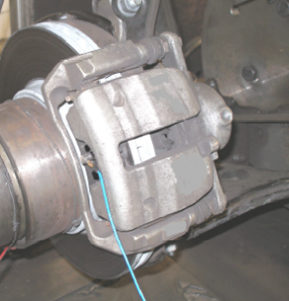
Figure 1: Brake system with accelerometer based on the backing plate of the brake pad mounted on commercial brake test rig.

The friction noise and vibration data has been obtained by an accelerometer on the backing plate of the outer brake pad. The sensor is an optimised piezoelectric type specified with a limiting frequency up to about 100 kHz in conjunction with a sample rate of the data acquisition above 200 kHz. The suppression of high frequency electromagnetic radiation effects has been assured by EMC-compatible countermeasures. In addition, the galvanic isolation of the chassis earth of the test set-up, the dynamometer itself, the data acquisition electronics, the dynamometer automation system as the trigger source and the isolation of the power electronics demanded further attention and arrangements. The acceleration signal of the sensor on the brake pad reflects the dynamics of the backing plate. The sensitivity of the applied sensor strongly decays above 95 kHz, but as the subsequent results suggest, also signal components beyond can be captured. The use of alternative measuring principles, like e.g. optical ones, in order to elevate the cut-off frequency had been accompanied by other problems, like e.g. coherence length effects of laser based approaches. Also the mechanically rough environmental conditions inside the dynamometer test chamber rendered the operation of an optical laser-doppler-system in the ultrasonic range impossible. As for the position of the sensor, in the following only results that do not depend on the specifics of the sensor location will be reported, and the sensor has been attached right in the middle of the backside of the brake pad’s backing plate, as can be seen from Figure 1. The resulting measurements typically yielded large data sets that have not been post-processed in any way, apart from the processing procedures inherent in the signal analysis techniques to be applied.

As for loading and environmental conditions, three different time-series will be investigated. All of them have been collected from what is called stop-braking in the industry: a constant brake line pressure is applied and the brake disk comes from an initial rotation to a full stop. For all the data, the initial disk rotation rate corresponds to a vehicle speed of 50 km/h. The first time-series, which we will call S3 subsequently, the brake pressure was 30 bar, and the initial disk temperature was 60 degrees Celsius. The second series, S2, has been obtained with 25 bar brake pressure and an initial disk temperature of 100 degrees, the third time series, S1, with 10 bar and an initial temperature of 100 degrees. The three cases have been obtained after typical but different braking test collectives had been run. The motivation for the selected sequence of tests is based on typical braking sequences during normal driving: a first strong brake application is often done with a comparatively cold brake. For the subsequent braking actions, the brake system is heated up due to the previous braking phases, and often softer brake application follows more severe one. Here we would like to mention that of course the present selection of time-series is a bit arbitrary. Many more and quite different loading cases and environmental scenarios would probably be worth while studying. However, the purpose of the present study is rather on showing the feasibility of applying alternative techniques of non-linear time-series analysis to friction vibration data, than on exhaustively analysing brake vibration in general, or even studying a given individual brake configuration completely. Therefore we hope that the results presented subsequently will prove convincing enough to initiate further work in the field.

It has already been shown previously [36, 37] that for each individual braking event the time evolution of the spectral characteristics of the generated vibration is quite stationary. We will thus not repeat the discussion on this behaviour here, but instead directly commence with the novel analysis techniques subject of the present study.

3 Methods for analysis of studied time series

First of all we note that if the investigated time series exhibit some periodicity, then the autocorrelation function has periodic behaviour too, while for chaotic or stochastic time series the autocorrelation function usually decays very fast. If long-range correlations are present, we can observe a power-law decay. The methods for investigating long-range correlations of long enough time series, such as WTMM (Wavelet Transform Modulus Maxima) method, DFA (Detrended Fluctuation Analysis) and MFDFA (Multi-fractal Detrended Fluctuation Analysis) have been intensively developed in the last decade. For more information on these methods and their applications, see for an example [41] - [45]. Subsequently we will give a very short introduction into the methods selected for the present purpose.

PCA and SSA can be most successfully used to analyse short and non-stationary time series in combination with the widely used method of construction of phase space by means of delay vectors [39, 40],[46]-[48], often called time-delay phase space construction (TDPSC). The idea of SSA-PCA-TDPSC is as follows. Let us have a time series consisting of $N^{*}$ values $x(\tau_{0}),x(2\tau_{0}),\dots,x(N^{*}\tau_{0})$ recorded by using fixed time step $\tau_{0}$. On the basis of the time series we construct $m-$dimensional vectors as follows. First we choose the step $\tau=n\tau_{0}$ and then we construct the vectors ($i=1,2,\dots,n$)

$$\vec{X}_{i}=\{x(i\tau_{0}),x(i\tau_{0}+\tau),\dots,x(i\tau_{0}+(m-1)\tau)\}$$

By means of the vectors $\vec{X}_{i}$ we build the trajectory matrix

$${\bf X}=\frac{1}{N^{1/2}}[\vec{X}_{1}^{T},\vec{X}_{2}^{T},\dots,\vec{X}_{N}^{T}]^{T}$$ (3.1)

and the covariance matrix of the trajectory ${\bf K}={\bf X}^{T}{\bf X}$. Let $\vec{k}_{p}$ be the eigenvectors of the covariance matrix and $\sigma_{p}$ the eigenvalues corresponding to these vectors. The vectors $\vec{k}_{p}$ form an orthonormal basis in the $m-$ dimensional space of the vectors $\vec{X}_{i}$. The matrix ${\bf X}$ can be decomposed as: ${\bf X}={\bf S}{\bf\Sigma}{\bf C}^{T}$ where ${\bf S}$ is an $N\times m$ matrix consisting of the eigenvectors of the trajectory matrix. ${\rm{\bf C}=[\vec{k}_{1},\vec{k}_{2},\dots,\vec{k}_{m}]}$ is an $m\times m$ orthogonal matrix and ${\bf\Sigma}={\rm diag[\sigma_{1},\sigma_{2},\dots,\sigma_{m}]}$ is the diagonal matrix constructed by the eigenvalues $\sigma_{i}$, also called singular values. These values are non-negative and the common rule is to number them in such a way that: $\sigma_{1}\geq\sigma_{2}\geq\dots\geq\sigma_{m}\geq 0$.

We can decompose the time series $\{x_{i}\}$ using the eigenvectors $\vec{k}_{q}$ of the Toeplitz matrix connected to the time series

$$x_{i+j}=\sum_{l=1}^{m}a_{i}^{l}k_{j}^{l},\hskip 14.22636pt1\leq j\leq m$$ (3.2)

The principal components $a_{i}^{l}$ of the time series can be obtained by a projection of the time series on the basis vectors

$$a_{i}^{l}=\sum_{j=1}^{m}x_{i+j}k_{j}^{l}$$ (3.3)

Thus SSA and PCA can be successfully combined with the TDPSC. This can be considered the first step in the procedure of time-delay embedding (TDE). TDE, however, underlies further restrictions. For an example, the dimension of the phase space as well as the time lag for construction of delay vectors on the basis of the stationary time series have to be chosen by strict procedures [49]-[53]. For the needs of SSA and PCA the requirements on TDPSC are much looser. One may e.g. choose a small delay (usually $\tau=\tau_{0}$, i.e. $n=1$ ) and large phase space dimension $m$ (as large as the investigated time series allows) [39].

Usually the principal components corresponding to the smaller singular values have small amplitude and oscillate with high frequency. Thus the information on large-amplitude slow periodic processes is compressed in the first principal components. In many cases, projection on the subspace of the first principal components can act as a reasonable filter to eliminate the usually low-amplitude and high-frequency processes to be neglected. In our case, one might expect the first components to catch the low-frequency structural dynamics, while the high-frequency interface processes could be expected to show up in the subsequent components. This filtering property of the PCA is very conveniet for the time-delay embedding methodology for estimation of characteristic quentities of the system dynamics on the basis of time series. The methodology requires noise-free time series for a good estimation of corresponding quantities. In many cases the PCA can be used as a noise filtering tool before application of the time-delay embeding methods. Such filtering will be used below. We note however that when we come to the application of the mulrtifractal detrended fluctuation analysis (in Sect. 5) we shall use the original time series and not the time series processed by the PCA.

In order to perform appropriately the above projection, we have to know the dimension of the subspace onto which we shall project our time series. This dimension is called the statistical dimension [12],[54] and it can be obtained in a heuristic fashion on the basis of the singular spectrum analysis (SSA). The singular spectra show us which principal components contain significant information for large amplitude and low frequency properties of the time series. Usually two situations arise:

• Presence of a kink in the singular spectrum.

  In many cases in the singular spectra we can observe that there exist several large values followed by a kink, i.e., the next singular values are much smaller then the first several ones. The number of large singular values can then be taken to determine the statistical dimension $S$ as the dimension of a principal components phase subspace to which the discussed above projection can be performed. Thus, if we observe a kink in the singular spectrum after a small number of singular values, a low-dimensional description of the characteristic features of the dynamics that underlies the time series is possible.

• There is no kink in the singular spectrum

  In this case the selection of the important principal components can be based on the requirement that the percentage of the total variance of the time series concentrated in the selected number of principal components must be larger than some prescribed value, say 90% or 95%. We have to expect that the dynamics of the system underlying the time series is probably very high-dimensional, i.e., with many significant degrees of freedom.

Thus even in the cases where no clear kink is visible in the spectrum of singular values, we can estimate a value of $S$ which can lead to a reasonable subspace projection and to a good model of the dynamics of the underlying system.

We note that the statistical dimension provides upper bound for the minimum degrees of freedom of the measured system [12]. It is an useful quantity but it is not a characteristic of the system itself and should not be confused with other dimensions that are independent on noise.

4 SSA and PCA analysis of the data

4.1 Influence of the sampling frequency

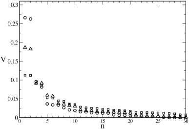
Figure 2: Influence of the sampling frequency on the variance connected to the principal components. Circles: sampling frequency of the original record. Triangles: sampling frequency is two times lower in comparison to the sampling frequency of the original record. Squares: sampling frequency is four times lower in comparison to the sampling frequency of the original record.

Fig. 2 shows the influence of the sampling frequency on the variance connected to the principal components of the different time series. The figure shows that the influence of the sampling frequency is quite strong. In principle one has to expect that the recorded time series will capture processes with a characteristic frequency up to the sampling frequency. Visual inspection of the results for the recorded data shows that in the case of the time series under investigation, the sampling frequency was just enough to capture all significant macro-scales. If we reduce two times the sampling frequency we lose substantial information: the variation at the largest principal components drops. This means that we lose significant informations hidden in the large time scales of the vibration processes connected with the brake event. If we reduce the sampling frequency further, the amount of the variance in the largest components drops further. In turn the amount of variance at the small-amplitude principal components increases.

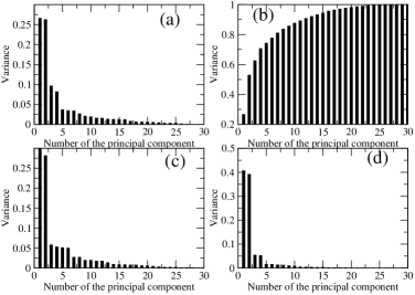
Figure 3: Variance connected to the principal components. Sampling frequency is the same as in the original record. Figure (a): time series S1. Figure (b): sum of the variances of the principal components for the time series S1. Figure (c): time series S2. Figure (d): time series S3.

Fig. 3 shows the values of the variance connected to the principal components of the investigated time series. As we can see from the Fig. 2b about 90% of the cumulative variance of the time series is contained in the largest 12 principal components. Thus we can use $S=12$ as statistical dimension of the time series S1. Similar is the situation with the time series S2. There $S=12$ too. The statistical dimension is much smaller for the time series S3, however. For this time series the $90\%$ of the variance is contained already in the first 6 principal components, i.e. $S=6$ here. This is an interesting result. One should remember that the time series S3 corresponds to a high pressure brake application in cold conditions, while time series S2 and S1 correspond to brake applications with lower pressures, but with higher initial temperatures. Since the individual braking cases had been extracted from within longer braking tests, it is difficult to pin down the origin of this behaviour further. Nevertheless, the analysis suggests that sometimes higher, and sometimes much lower statistical dimensions may result.

With respect to the primary objective of this study, these are quite remarkable findings. First of all the results show that there is a surprisingly small number of dominant dimensions, most likely related to the low-frequency structural dynamics of the system, capturing most of the relevant dynamics of the overall processes, at least in the somehow energetic sense of variance. Second, these low-frequency effects are intricately coupled to the rest of the dynamics, and even the very high sampling rates, which are about a magnitude higher than what simple reasoning based on the limits of the audible range would suggest, do not seem completely sufficient to separate the slow processes of structural dynamics from the fast processes, that most likely are generated in the friction interface itself. Of course, also here it needs to be stressed that the data basis for this study has been comparatively small, with only three time-series at hand. More work with more extended data will thus be needed before further conclusions can be drawn.

4.2 Embedding after projection

To further characterise and quantify the data, we use the dominant principal components as base vectors and project the time series on the subspace of the principal components corresponding to largest singular values. The information for large-amplitude slow processes is by this compressed into the largest principal components. In order to perform appropriately the above projection, we have to know the dimension of the subspace onto which we shall project our time series. This dimension is the statistical dimension $S$ calculated above.

After the projection onto the principal components we can investigate the chaotic characteristics of the time series (filtered from the remaining dynamics by the projection on the largest principal components). In order to do this we shall use the time-delay embedding procedure described below. Before we start let us note that this procedure doen’t lead to one-to-one image of the corresponding chaotic attractor. The procedudure preserves some topological properties of the attractor due to the inverainat measures. Some of these measures will be obtained below.

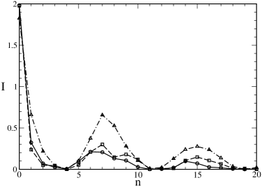
Figure 4: The mutual information $I(n)$. Solid line: S1. Dashed line: S2. Dot-dashed line: S3.

In order to perform embedding we need appropriate values of the time-delay and of the embedding dimension. A candidate value for the time delay can be obtained on the basis of the quantity called mutual information [55]

$$M=-\sum_{i,j}p_{ij}(\tau)\ln\frac{p_{ij}(\tau)}{p_{i}p_{j}}$$ (4.1)

In order to use Eq.(4.1) one has to make a partition of the values of the time series. Then $p_{i}$ is the probability to find a time series value in the $i$-th interval of the partition. $p_{ij}$ is the joint probability that if an observed values falls in the $i$-th interval of the partition then the value observat at time $\tau$ later falls in the $j$-th interval of the partition.

Figure 4 shows the results for the calculation of the mutual information of the investigated projected time series. A good candidate for the delay time in the time-delay embedding procedure is obtained from the first minimum of the mutual information. One can see that for all time series a good candidate for time delay is $t_{delay}=4$ sampling intervals which corresponds to $2\cdot 10^{-5}$ s.

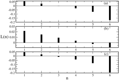
Figure 5: The largest 6 Lyapunov exponents for the time series (Sano-Sawada method). Figure (a): time series S1. Figure (b): time series S2. Figure (c): time series S3.

Next we have to obtain the minimum embedding dimension. For this we shall use the concept of the false nearest neighbours [56]. Let the minimum embedding dimension for the investigated time series be $m$. In the corresponding $m$-dimensional delay space the reconstructed attractor will be a one-to-one image of the attractor in the original phase space and the topological properties will be preserved. In other words the neighbours of a given point are mapped onto neighbours in the delay space and neighbourhoods of the points are mapped onto neighbourhoods again. If the embedding is in delay space of dimension $m^{*}<m$ then the projection the topological structure is no longer preserved. Points are projected into neighbourhoods of other points to which they wouldn’t belong in higher dimensions. These points are called false neighbours. Then if we increase the dimension $m^{*}$ of the delay space the number of the false neighbours will decrease and when we reach the desired dimension $m$ the number of the false neighbours will be very small. Following this algorithm, we have obtained the following values of $m$ for our time series

• Time series S1: $m=10$

• Time series S2: $m=12$

• Time series S3: $m=6$

Confirming earlier findings based on different techniques [36], the results again suggest that most of the dynamics is indeed captured within comparatively low-dimensional deterministic dynamics. Although from a purely data focussed perspective this finding might not be too surprising, for the mechanical engineer and a structural dynamics point of view this finding is rather counter-intuitive. The spectral or modal perspective on the vibration properties of a large technical structure like a friction brake would usually feed the expectation that the broad band interface processes would excite a large number of vibration modes of the system. And even within the audible range itself, there would be thousands of modes available to be excited. However, the present findings suggest that the structural dynamics is dominated by a very low-dimensional (sub-)system only.

Additional evidence about the low-dimensionality of the dynamics is obtained by means of correlation dimension. Correlation dimension $D_{2}$ [57], [58] is a measure of the dimensionality of the space occupied by a set of random points. For calculation of this dimension we have used the TISEAN package [39]. The results for the investigated time series are as follows

• Time series S1: $D_{2}=3.54$;

• Time series S2: $D_{2}=5.43$;

• Time series S3: $D_{2}=3.08$.

4.3 Lyapunov exponents and the Kaplan-Yorke dimension

The maximum Lyuapunov exponents for the time series have been calculated. The values are shown in Table 1. Moreover the spectrum of the Lyapunov exponents has been determined on the basis of the methodology from [59], [60]. The results are presented in Fig. 5. We can see that for all time series there are at least two positive Lyapunov exponents. The presence of one positive Lyapunov exponent with the second largest exponent equal to $0$ is already an indicator for the presence of chaos. When more than one positive Lyapunov exponent exists, one sometimes talks about hyper-chaos, which seems to be the case here.

Time series	Maximum Lyapunov exponent	Kaplan-Yorke dimension
Time series S1	$L_{max}=0.055$	$D_{KY}=3.76$
Time series S2	$L_{max}=0.021$	$D_{KY}=5.74$
Time series S3	$L_{max}=0.043$	$D_{KY}=3.32$

Table 1: Maximum Lyapunov exponents and Kaplan-Yorke dimensions for the studied time series.

The calculation of the spectrum of Lyapunov exponents allows us also to calculate the Kaplan-Yorke dimension of the underlying attractors:

$$D_{KY}=k+\frac{\sum_{i=1}^{k}L_{i}}{\mid L_{k+1}\mid}$$ (4.2)

where $k$ is the maximum integer such that the sum of the $k$ largest Lyapunov exponents is still non-negative. Here one has to deal with the problem of spurious Lyapunov exponents. The problem arises from the fact that the rconstructed phase space has extra dimensions compared to the true phase space of the corresponding physical system. This leads to extra, so called spurious Lyapunov exponents. Recently Yang, Radons, and Kantz [61], [62] have used the concept of covariant Lyapunov vectors for identification of spurious Lyapunov exponents. The covariant Lyapunov vectors can be calculated on the basis of algorithm proposed in [63]. Application of this methodology leads to the Kaplan-Yorke dimensions for the time series are shown in the third column of Table 1. What is interesting is that the Kaplan-Yorke dimension jumps for the time series S2 and has close values for the other two time series. Again, very small numbers result, which first of all indicates that the present analysis and projection approach has been successful.

Again, with respect to the mechanical dynamical system under study, however, the smallness of the attractors dominating the slow structural vibration dynamics is surprising: in engineering dynamics irregular vibration states are usually thought to be caused by truly high-dimensional processes, accessible through statistical rather than deterministic analysis. The vibration response of the structure of a system is generally thought to be such that a large number of degrees of freedom will be involved, when the forcing becomes complex. This way of thinking seems to be originating in the traditional picture of engineering systems to be composed of a large number of undamped and uncoupled oscillators. The present analysis suggests that in fact the resulting dynamics is far less complex in terms of active degrees of freedom than what one could naively think from plainly counting discrete modes in frequency space, or nodes of a geometry capturing finite element representation. While the appearance of such low-dimensional deterministic kernels in complex dynamics seems to have been widely accepted for long time in the sciences, in engineering there is hardly any data based proof for it in technical systems. This is why the present system might be of special interest and importance to the field.

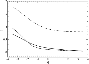
Figure 6: $h(q)$ spectra for the time series. Solid line: S1. Dashed line: S2. Dot-dashed line: S3.

5 Multifractal detrended fluctuation analysis (MFDAFA) of the time series

5.1 The MFDFA methodology

Experience, and also the subsequent results, show that the above approach yields interesting insights into the dominant slow time-scale and low frequency dynamics, related to the vibrations of the structure. A complementary perspective would be to focus on the dynamical processes taking place at the friction interface itself, and possibly the interactions between these usually multi-scale processes with the comparatively slow structural dynamics. For that purpose, we here employ multi-fractal detrended fluctuation analysis (MFDFA), which has proven highly successful in a number of other scientific disciplines [41], [64], [65]. The idea here is to investigate the long-range correlations in the inter-maxima intervals in the time series and analyse its correlation properties.

The long range correlations in time series can be investigated on the basis of Hurst exponent [66], [67]. When the time series are obtained on the basis of Brownian motion then the Hurst exponent ie equal to $0.5$. When the process is persistent the Hurst exponent is larger than $0.5$. When the process is anti-persistent the Hurst exponent is smaller than 0.5. For white noise the Hurst exponent is 0 and for a simple linear trend the exponent is 1.

If we have time series with appropriate scaling properties by means of MFDFA we can calculate the spectrum $h(q)$ of the local Hurst exponent [41]. Then we obtain the exponent $\alpha$ and the fractal spectrum $f(\alpha)$ by means of the relationships

$$\alpha=h(q)+q\frac{dh}{dq},\hskip 14.22636ptf(\alpha)=q[\alpha-h(q)]+1$$ (5.1)

as well as the mass exponent $\tau_{q}$

$$\tau_{q}=qh(q)-1$$ (5.2)

The mass exponent supplies evidence for the multifractality of the investigated time series. The monofractal time series has mass exponent $\tau_{q}$ with a linear $q$-dependence. $\tau_{q}$ with a nonlinear $q$-dependence is evidemce for multifractality.

The realization of the MFDFA method is as follows [41] (see also [42]-[45]). First of all, on the basis of the time series $\{x_{k}\}$, we calculate the profile function

$$Y_{i}=\sum_{k=1}^{i}(x_{k}-\langle x\rangle),\hskip 14.22636pti=1,2,\dots,N$$ (5.3)

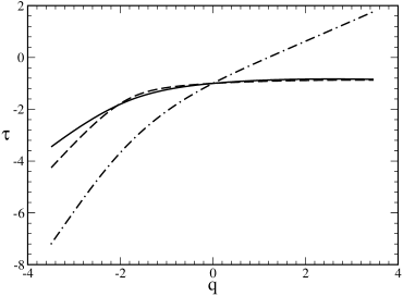
Figure 7: $\tau(q)$ spectra for the time series. Solid line: S1. Dashed line: S2. Dot-dashed line: S3.

Then we divide the time series into $N_{s}={\rm int}(N/s)$ segments and calculate the variation of each segment. As the segments will not include some data at the end of the time series we add additional $N_{s}$ segments, which start from the last value of the time series in the direction of the first value of the series. In order to calculate the variation we have to calculate the local trend (the fitting polynomial $y_{\nu}(i)$) for each segment of length $s$ where $s$ is between some appropriate minimum and maximum values. The variation is

$$F^{2}(\nu,s)=\frac{1}{s}\sum_{i=1}^{s}\{Y[(\nu-N)s+i]-y_{\nu}(i)\}^{2},$$ (5.4)

for the first $N_{s}$ segments and

$$F^{2}(\nu,s)=\frac{1}{s}\sum_{i=1}^{s}\{Y[N-(\nu-N)s+i]-y_{\nu}(i)\}^{2},$$ (5.5)

for the second $N$ segments. Finally we obtain the $q$-th order fluctuation function by averaging over all segments as follows

$$F_{q}(s)=\left\{\frac{1}{2N_{s}}\sum\limits_{\nu=1}^{2N_{s}}\bigg{[}F^{2}(\nu,s)\bigg{]}^{\dfrac{q}{2}}\right\}^{\dfrac{1}{q}}.$$ (5.6)

The scaling properties of $F_{q}(s)$ determine the kind of fractal characteristics of the time series. For mono-fractal time series $F_{q}(s)$ scales as $s$ of constant power $h$ for each $q$. For sequences of random numbers $h=1/2$. If $s>>s^{*}$ this value of $h$ would be unchanged even in presence of local correlations extending up to a characteristic range $s^{*}$. If the correlations do not have characteristic length $h$ will be different from $1/2$. If the time series exhibit multi-fractal properties (up to the the smallest value of $s$) the exponent $h$ is not a constant and becomes a function of the parameter $q$: $h=h(q)$.

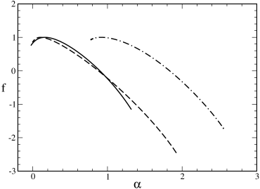
Figure 8: $f(\alpha)$ spectra for the time series. Solid line: S1. Dashed line: S2. Dot-dashed line: S3.

5.2 Results

Having obtained the above results on the dynamics underlying the slow time-scales, we now turn to the multi-fractal analysis of the time series to gain further insight into the dynamics from a complementary perspective. Our goal is just to show that the investigated kind of time series possess multifractal characteristics. The $h(q)$ spectra of the time series S1, S2, and S3 are presented in Fig.6. We observe that $h$ depends on $q$ which means that the time series exhibit multifractal properties up to smallest time scales recorded. In addition we observe some separation between the spectra for S3 on one side, and the spectra for time series S1 and S2 from the other side. This can be seen for an example in Fig. 7 for the $\tau(q)$ spectra, in Fig. 8 for the $f(\alpha)$ spectraq and in Fig. 9 for the $\alpha(q)$ spectra. Probably this means that the processes recorded in S1 and S2 are similar on a large number of scales, whereas there is something different or additional happening for the case of S3.

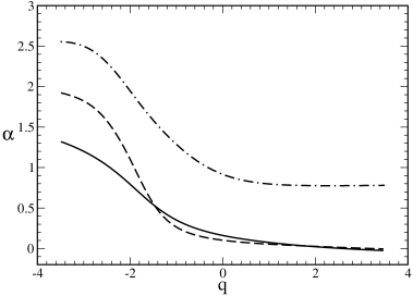
Figure 9: $\alpha(q)$ spectra for the time series. Solid line: S1. Dashed line: S2. Dot-dashed line: S2.

6 Concluding remarks

In this study we have analysed vibration data of a friction brake under normal operation. Accelerations at a given but arbitrary point on one of the brake pads have been measured with a sampling rate of 200 kHz. The recorded time-series have been subjected to a deliberate selection of techniques from non-linear time-series analysis. Singular spectrum analysis (SSA) has been combined with principal component analysis (PCA) and time delay phase space construction (TDPSC). Moreover a multi-fractal detrended fluctuation analysis (MFDFA) has been conducted. SSA based PCA and TDPSC suggest that the measured data clearly manifests a very small number of dominant components, corresponding to the low-frequency structural dynamics. Embedding analysis and calculation of Lyapunov exponents and attractor dimensions moreover shows that within the dominant subspace, the dynamics can well be characterised as chaotic, with attractor dimensions well below 10. The higher principal components show a rather smooth distribution, indicating the multi-scale nature of the faster processes originating by the sliding dynamics in the friction interface. The multi-fractal detrended fluctuation analysis (MFDFA) confirms the multi-scale character of the faster processes.

The results suggest a number of interesting conclusions that need to be discussed. First, although the time-series obtained do seem to represent random processes at first sight, it turns out that by the comparatively simple techniques applied the underlying dynamics may easily be separated into a low-dimensional deterministic core for the slow, low-frequency part, and a complex multi-scale part. Of course the separation is in no way trivial, and our analysis also shows that the data acquisition should indeed be expanded to even higher frequencies to capture an even larger part of the multi-scale processes. Nevertheless, a clear distinction between a small number of dominant low-frequency degrees of freedom and separate multi-scale processes can already be drawn from the present analysis. Second, the techniques presented might not only be used as tools to allow further insight into the nature of sliding friction, but might also be applied to characterise for example brake pad materials or operating conditions. The techniques applied yield a wealth of quantitative results that might well be hoped to be useful in system or load characterisation.

Future work might have a number of directions. First, the measurement basis has to be expanded and even higher sampling frequencies are desirable, also with multi-point measurements. Modelling and simulation approaches consistent with the present findings should be developed and model reduction approaches derived. But most importantly we hope that extended approaches along the lines used here will contribute to a better understanding of the today still largely unknown or poorly understood dynamical processes in interfaces, i.e. friction behaviour in general.

Finally let us note that the discussed above results have been obtained by the help of many computer programs. We have used the software of TISEAN package [39] as well as our own software for multi fractal detrended fluctuation analysis of time series.

References

- [1] A. C. Scott. Nonlinear science. Emergence and dynamics of coherent structures. Oxford University Press, Oxford, 1999.
- [2] J. D. Murray. Lectures on nonlinear differential equation models in biology. Oxford University Press, Oxford, 1977.
- [3] M. Ablowitz, P. A. Clarkson. Solitons, nonlinear evolution equations and inverse scattering. Cambridge University Press, Cambridge, 1991.
- [4] N. K. Vitanov, I. P. Jordanov , Z. I. Dimitrova. On nonlinear population waves. Applied Mathematics and Computation. 215, 2009, 2950 – 2964.
- [5] N. Martinov, N. Vitanov. On the correspondence between the self-consistent 2D Poisson-Boltzmann structures and the sine-Gordon waves. J. Phys. A: Math. Gen., 25, 1992 L51 – L56.
- [6] N. Martinov, N. Vitanov. On some solutions of the two-dimensional sine-Gordon equation. J. Phys. A: Math. Gen., 25, 1992, L419 – L426.
- [7] N. Martinov, N. Vitanov. Running-wave solutions of the two-dimensional sine-Gordon equation. J. Phys. A: Math. Gen., 25, 1992, 3609 – 3613.
- [8] N. K. Martinov, N. K. Vitanov. New class of running-wave solutions of the 2+1-dimensional sine-Gordon equation. J. Phys. A: Math. Gen., 27, 1994, 4611 – 4618.
- [9] N.K. Vitanov. On traveling waves and double-periodic structures in two-dimensional sine-Gordon systems. J. Phys. A: Math. Gen., 1996, 29, 5195 – 5207.
- [10] N.K. Vitanov, N. K. Martinov. On the solitary waves in the sine-Gordon model of the two-dimensional Josephson junction. Zeitschrift für Physik B: Cond. Matt.,100, 1996,129 – 135.
- [11] N. A. Kudryashov. Exact solutions of the generalized Kuramoto - Sivashinsky equation. Phys. Lett. A 147, 1990, 287 – 291.
- [12] Vautard R., Ghil M. Singular spectrum analysis in nonlinear dynamics with application to paleoclimatic time series. Physica D 1989; 35: 395-424.
- [13] Vautard R., Yiou P., Ghil M. Singular spectrum analysis - a tookit for short noisy chaotic signals. Physica D 1992; 58: 95-126.
- [14] Vitanov N. K., Sakai K., Dimitrova Z. I. SSA, PCA, TDPSC, ACFA: Useful combination of methods for analysis of short and nonstationary time series. Chaos Solitons & Fractals 2008; 37: 187-202
- [15] Panchev S., Spassova T., Vitanov N. K. Analytical and numerical investigation of two Lorenz-like dynamical systems. Chaos Solitons & Fractals 2007; 33: 1658-1671.
- [16] Schlesinger M. E., Ramankutty. An oscillation in the global climate system of period 65-75 years. Nature 1994; 367: 723-726.
- [17] Kravtsov S., Ghil M. Interdecadal variability in a hybrid coupled ocean-atmosphere-sea
- [18] Marelli L., Bilato R., Franz P., Martin P., Murari A., O’Gorman M. Singular spectrum analysis as a tool for plasma fluctuations analysis. Review of Scientific Instruments 2001; 72: 499-502.
- [19] Theobald C. M., Glassey C. A., Horgan G. W., Robinson C. D. Principal component analysis of landmarks from reversible images. Journal of the Royal Statistical Society C - Applied Statistics 2004; 53: 163-175.
- [20] Wold S., Esbensen K., Geladi P. Principal component analysis. Chemometrics and Intelligent Laboratory Systems 1987; 2: 37-52.
- [21] Carland J. L., Mills A. L. Classification and characterization of heterothropic microbial communities on the basis of patterns of community-level sole-carbon-source utilization. Applied and Environmental Microbiology 1991; 57, 2351-2359.
- [22] Russell E. L., Chiang L. H., Braatz R. D. Fault detection in industrial processes using canonical variate analysis and dynamic principal component analysis. Chemometric and Intelligent Laboratory Systems 2000; 51: 81-93.
- [23] Kantz H., Schreiber T. Nonlinear time series analysis. Cambridge: Cambridge University Press, 1997.
- [24] Böck T., Vitanov N. K. Low dimensional chaos in zero-Prandtl-number Benard Marangoni convection. Phys. Rev. E 2002; 65: Art. No. 037203.
- [25] Kantz H., Holstein D., Ragwitz M., Vitanov N. K. Markov chain model for turbulent wind speed data. Physica A 2004; 342: 315-321.
- [26] Dimitrova Z. I., Vitanov N. K. Chaotic pairwise competition. Theoretical Population Biology 2004; 66: 1-12.
- [27] Vitanov N. K., Dimitrova, Z. I., Kantz H. On the trap of extinction and its elimination. Phys. Lett. A 2006; 349: 350-355.
- [28] Kinkaid N. M., O’Reilly O.M., Papadopoulos P. Automotive disc brake squeal. Journal of Sound and Vibration 2003; 267: 105-166.
- [29] Chen F. Automotive disk brake squeal: an overview. International Journal of Vehicle Design 2009; 51: 39-72.
- [30] Hoffmann N., Gaul L. Friction induced vibrations of brakes: research fields and activities. SAE Technical Paper Series 2008; 2008-01-2579: 1-8.
- [31] Diao K., Zhang L., Meng D. Study on Statistical Analysis of Uncertainty of Disc Brake Squeal. SAE Technical Paper 2014-01-0030.
- [32] Diao K., Zhang L., Meng D. Modeling and Experimental Investigation on Time-varying Characteristic of Brake Frictional Squeal. SAE Technical Paper 2014-01-2517.
- [33] Feeny B. F, Liang J. W. Phase Space Reconstructions and Stick-Slip. Nonlinear Dynamics 1997; 13: 39-57.
- [34] Oberst S., Lai J. C. S. Chaos in brake squeal noise. Journal of Sound and Vibration 2011; 330: 955-975.
- [35] Oberst S., Lai J. C. S. Statistical analysis of brake squeal noise. Journal of Sound and Vibration 2011; 330: 2978-2994.
- [36] Wernitz B. A., Hoffmann N. P. Recurrence analysis and phase space reconstruction of irregular vibration in friction brakes: Signatures of chaos in steady sliding. Journal of Sound and Vibration 2012; 331: 3887-3896.
- [37] Wernitz B. A., Hoffmann N. P. New Approaches to Signal Analysis of Friction Noise and Vibration. Proc. IMechE International Conference of Braking; York 2009.
- [38] Kappagantu R. V, Feeny B. F. Part 1: Dynamical Characterization of a Frictionally Excited Beam. Nonlinear Dynamics 2000; 22: 317-333.
- [39] Hegger R., Kantz H., Schreiber T. Practical implementation of nonlinear time series methods: The TISEAN package. CHAOS 1999; 9: 413-435
- [40] Schreiber T. Interdisciplinary applications of nonlinear time series methods. Physics Reports 1999; 308: 2-64.
- [41] Kantelhard J. W., Koscielny-Bunde E., Rego H. H. A., Havlin S., Bunde A. Detecting long-range correlations with detrended fluctuation analysis. Physica A 2001; 295: 441-454.
- [42] Kantelhardt J. W., Zschiegner S. A., Koscielny-Bunde E., Havlin S., Bunde A., Stanley HE. Multifractal detrended fluctuation analysis of nonstationary time series. Physica A 2002; 316: 87-114.
- [43] Ivanov P. C., Amaral L. A. N., Goldberger A. L., Havlin S., Rosenblum M. G., Struzik Z. R., Stanley H. E. Multifractality in human heartbeat dynamics. Nature 1999; 399: 461-465.
- [44] Muzy J. F., Bacry E., Arneodo A. The multifractal formalism revisited with wavelets. Int. J. Bif. Chaos 1994; 4: 245-302.
- [45] Vitanov N. K., Yankulova E. D. Multifractal analysis of the long-range correlations of the heartbeat activity of Drosophila melanogaster. Chaos Solitons & Fractals 2006; 28: 768-775.
- [46] Broomhead D. S., King G. P. Extracting qualitative dynamics from experimental data. Physica D 1986; 20: 217-236.
- [47] Albano A. M., Muench J., Schwant C., Mees A. I., Rapp P. E. Singular-value decomposition and the Grassberger-Procaccia algorithm. Phys. Rev. A 1988; 38: 3017-3026.
- [48] Mees A. I., Rapp P. E., Jennings L. S. Singular-value decomposition and embedding dimension. Phys. Rev A 1987; 36: 340-346.
- [49] Sauer T., Yorke J. A., Casdagli M. Embedology. J. Stat. Phys. 1991; 65: 579-616.
- [50] Abarbanel H. D. I., Brown R., Sidorowich J. J., Tsirming L. S. The analysis of observed chaotic data in physical systems. Rev. Mod. Phys. 1993; 65: 1331-1392.
- [51] Farmer J. D., Sidorowich J. J. Predicting chaotic time series. Phys. Rev. Lett. 1987; 59: 845-848.
- [52] Kantz H., Schreiber T. Dimension estimates and physiological data. CHAOS 1995; 5: 143-154.
- [53] Hegger R., Kantz H., Matassini L., Schreiber T. Coping with nonstationarity by overembedding. Phys. Rev. Lett. 2000; 84: 4092-4095.
- [54] Elsner J. B., Tsonis A. A. Singular spectrum analysis. A new tool in time series analysis. New York: Springer, 1996.
- [55] Fraser, A. M., Swinney H. L. Independent coordinates for strange attractors from mutual information. Phys. Rev. A 1986; 33: 1134-1140.
- [56] Kennel M. B., Brown R., Abarabanel H. D. I. determining embedding dimension for phase-space reconstruction using a geometrical construction. Phys. Rev. A 1992; 45: 3403-3411
- [57] Grassberger P., Procaccia I. Measuring the strangeness of strange attractors. Physica D 1983; 9, 189-208.
- [58] Sauer T., Yorke J. How many delay coordinates do you need? Int. J. Bifurcation and Chaos 1993; 3, 737-744.
- [59] Sano M., Sawada Y. Measurement of the Lyapunov spectrum from a chaotic time series. Phys. Rev. Lett. 1985; 55: 1082-1085.
- [60] Eckmann J.-P., Ollifson Kamphorst S., Ruelle D., Ciliberto S. Lyapunov exponents from a time series. Phys. Rev. A 1986; 34: 4971-4979.
- [61] Yang H.-L., Radons G., Kantz H. Covariant Lyapunov vectors from reconstructed dynamics: The geometry behind true and spurious Lyapunov exponents. Phys. Rev. Lett. 2012; 109, Article No. 244101.
- [62] Kantz H., Radons G., Yang H.-L. The problem of spurious Lyapunov exponents in time series analysis and its solution by covariant Lyapunov vectors. J. Phys. A: Math. Theor. 2013; 46, Article No. 254009.
- [63] Ginelli F., Poggi P., Turchi A., Chate H., Livi R., Politi A. Characterizing dynamics with covariant Lyapunov vectors. Phys. Rev. Lett. 2007; 99, Article No. 130601.
- [64] Lopez J. L., Veleva L., Lopez-Sauri D. A. Multifractal detrended analysis of the corrosion potential fluctuations during copper patina formation on its first stages in sea water. International Journal of Electrochemical Science 2014; 9, 1637-1649.
- [65] Murgia J. S., Rosu H. S. Multifractal analysis of row sum signals of elementary cellular authomata. Physica A 2012; 391, 3638-3649.
- [66] Bassingthwaighte J. B., Liebovitch L. S., West B. J. Fractal psychology. New York: Oxford University Press, 1994.
- [67] Sanchez Cranero M. A., Trinidada Segovai J. E., Garzia Perez J. Some comments on Hurst exponent and the long memory processes on capital markets. Physica A 2008; 387, 5543-5551.