Advancements in the ADAPT Photospheric Flux Transport Model

Abstract

Global maps of the solar photospheric magnetic flux are fundamental drivers for simulations of the corona and solar wind and therefore are important predictors of geoeffective events. However, observations of the solar photosphere are only made intermittently over approximately half of the solar surface. The Air Force Data Assimilative Photospheric Flux Transport (ADAPT) model uses localized ensemble Kalman filtering techniques to adjust a set of photospheric simulations to agree with the available observations. At the same time, this information is propagated to areas of the simulation that have not been observed. ADAPT implements a local ensemble transform Kalman filter (LETKF) to accomplish data assimilation, allowing the covariance structure of the flux transport model to influence assimilation of photosphere observations while eliminating spurious correlations between ensemble members arising from a limited ensemble size. We give a detailed account of the implementation of the LETKF into ADAPT. Advantages of the LETKF scheme over previously implemented assimilation methods are highlighted.

Keywords: Solar magnetic fields, Photosphere, Data assimilation

1 Introduction

The dynamic magnetic fields of the Sun, from coronal holes to strong photospheric magnetic fields within active regions, play a central role in driving Earth’s space environment. The global solar photosphere represents the boundary conditions for corona and solar wind models. Therefore, accurately establishing the global solar photospheric magnetic field provides a better understanding and specification of Earth’s space weather environment.

Solar magnetic field measurements are recorded on a regular basis for half the solar surface, e.g. the National Solar Observatory (NSO) Global Oscillation Network Group (GONG) [19] and the Helioseismic and Magnetic Imager (HMI): [35] onboard the Solar Dynamics Observatory (SDO). Additional efforts are being made to use helioseismic techniques to estimate active regions on the far side of the Sun by analyzing acoustic waves propagating from the far side of the Sun to the Earth side [29]. The Solar Terrestrial Relations Observatory (STEREO); [39] mission from NASA has provided $360^{\circ}$ observations from the solar corona, making it the first ever data set that provides an almost complete nowcast (estimate of the current state) of the solar corona. Additionally, methods of reconstructing the Sun’s coronal dynamics from observation have been advancing [10]. Although many of these observational data sets provide an accurate estimation of the current state of a portion of the solar photosphere’s magnetic flux, we lack the magnetograph observations needed to generate an instantaneous map of the global photospheric magnetic flux distribution.

Data assimilation methods are techniques that fuse information from observational data into a physics-based model in order to align the model with current physical conditions and improve forecasts [11, 26]. The ensemble assimilation methods discussed in this article are sequential, as opposed to variational, and work by first randomly initializing several realizations of a solar model; this is referred to as the ensemble. Next, the ensemble members are propagated forward in time until a physical observation is made. Each ensemble member then contributes a simulated observation and these observations are compared with the physical observation. Lastly, the ensemble members are adjusted by weighting the physical observation’s noise and the ensemble of simulated observation’s variance. After the adjustment is performed, the analyzed ensemble is propagated forward in time again until the next physical observation is made and the process is repeated. The large variety of data assimilation methods specify the different forms for the adjustment that should be performed on the ensemble.

Assimilation methods are starting to be implemented into solar modeling to enable a better nowcast and forecast from a wide range of models [8]. For example, [10] utilize the ensemble Kalman filter along with a tomography method to reconstruct the dynamic solar corona from real observational data and a random walk model of coronal dynamics, [27] also utilized the ensemble Kalman filter to forecast the solar cycles and sunspot number by combining real observations with a reduced $\alpha\Omega$-dynamo model, while [5] used the four-dimensional variational method (4D-Var) and a cellular-automaton-based avalanche model to predict simulated solar flare data. A variational data assimilation technique was developed by [25] using an $\alpha\Omega$-dynamo model for the Sun; their techniques were validated using synthetically generated data. [40] applied a three-dimensional variational (3D-Var) data assimilation methodology for a two-dimensional convection flow to simulated observations. An ensemble Kalman filter method was implemented in a Babcock–Leighton solar dynamo model, using synthetic data, by [12]. Observations were combined with a physical model by [13] who used and assimilation technique consisting of a simple data-nudging method. The mentioned works illustrate just a few examples of a wide range of problems from solar modeling that utilize data assimilation methods. In this work, three different ensemble Kalman methods are compared as data assimilation techniques for combining a physical model of the flux transport dynamics of the solar photosphere and real vector spectral magnetograph (VSM) observations. To the authors’ knowledge, this represents the first comparison of multiple sophisticated assimilation methods using a physical solar photosphere model and real observations.

The Air Force Data Assimilative Photospheric Flux Transport (ADAPT) Model [3, 4, 22, 2] incorporates various data assimilation techniques, using a module developed at Los Alamos National Laboratory (LANL) [3], with a photospheric magnetic flux transport model. The ADAPT model is updated with observations by using an ensemble of simulations from a flux transport model based on the method used in the Worden–Harvey (WH) model [44] to represent the distribution of possible solar photospheric states under the influence of differential rotation, meridional flow, supergranular diffusion, and random emergence of weak background flux. The ensemble information is then used in LANL’s ensemble Kalman filter (ENKF) data assimilation method to adjust the ADAPT model using observational data. The adjustment is made by comparing the covariance structure of the model, as computed from the ensemble samples, with an observation and its noise. In areas where the ensemble shows a diffuse distribution, representing lack of determination in the model, observations have a greater impact on the ensemble. Several types of Kalman filtering techniques are now available for use with the ADAPT model. To date all data assimilation methods implemented with ADAPT are sequential as opposed to variational methods. Specifically the most recent LANL module’s data assimilation method in ADAPT implements a localized version of ensemble Kalman filtering, which assimilates each observation within a local region of the model spatial field. This localization allows approximation of the ADAPT spatial covariance structure to effect the assimilation of new observations more effectively. At the same time the localization in the data assimilation eliminates erroneous long distance correlations occurring from the small sample sizes used to estimate the ADAPT model’s covariance structure. It is worth noting that all ADAPT maps and results to date have utilized an ensemble least squares (ENLS) data assimilation method [4, 22], whereas the ENKF data assimilation methods developed at Los Alamos have only been used so far in a testing and development capacity.

The article is outlined as follows: In Section 2 we give a brief description of the flux transport method within the ADAPT model and detail the implementation of the data assimilation scheme. This is followed by a comparison of different data assimilation methods available in ADAPT in Section 3. The article concludes, in Section 4, with a discussion of future directions for the ADAPT model.

2 Methods

2.1 Flux Transport within ADAPT

The photospheric flux transport within the ADAPT model is based on the Worden–Harvey (WH) model [44], which includes the effects of differential rotation, meridional flow, supergranulation, and random background flux. New flux emergence is added to the ADAPT simulation through data assimilation of observations. Mechanisms for the creation and destruction of large scale active regions remains an important research topic [9, 1, 47] but a definitive model has yet to emerge.

The rate of rotation of the photospheric flux is dependent on latitude. The sidereal rotation rate, at latitude $\theta$, is given by

$$\omega(\theta)=A+B\sin^{2}(\theta)+C\sin^{4}(\theta).$$ (2.1)

The original WH model used parameter values from Snodgrass [38], i.e. $A=2.902\,\mu\textrm{rad}/\mathrm{s}$, $B=-0.464\,\mu\textrm{rad}/\mathrm{s}$, $C=-0.328\,\mu\textrm{rad}/\mathrm{s}$. Currently the ADAPT model uses parameter values from [28], $A=2.913\,\mu\textrm{rad}/\mathrm{s}$, $B=-0.405\,\mu\textrm{rad}/\mathrm{s}$, $C=-0.422\,\mu\textrm{rad}/\mathrm{s}$.

ADAPT also includes a (mostly poleward) meridional flow that is more difficult to estimate from observations than is the nearly steady surface differential rotation. Difficulty in meridional flow estimation is due in large part to the flow rate being slow enough that it is difficult to distinguish from other transport processes such as supergranular flows. Moreover, there is evidence of significant meridional flow rate variation over the course of the solar cycle [20]. The ADAPT model uses the profile, based on [42], implemented in the original WH model given by

$$M(\theta)=(8\,m/\mathrm{s})|\sin(\theta)|^{0.3}|\cos(\theta)|^{0.1}.$$ (2.2)

This profile does not match observations, especially at lower latitudes, however, with regular observational data assimilated into ADAPT only the high latitudes ($|\theta|>65^{\circ}$) are affected by Equation (2.2).

The diffusion of flux is approximated with supergranular flows. ADAPT uses a stochastic diffusion method developed by [31] and [37] to simulate the diffusion and transport of supergranules. The stochastic diffusion used by ADAPT is based on the description in [44]. This representation of supergranular diffusion overestimates dissipation [44, 30], so the supergranular diffusion process is shut off in ADAPT for field strengths greater than $15$ to $50$ G depending on the data source and the rate of assimilation.

As noted in the original WH model, [36] point out that the photospheric magnetic flux would disappear due to random cancellations in two to three days if the total magnetic flux were not renewed regularly. For this reason the ADAPT framework includes daily random background flux emergence. This is accomplished by taking Gaussian distributed random flux at each pixel with mean zero and absolute mean value of $2.1$ G in each day of the simulation. This value of random flux emergence maintains a constant level of total flux in the synoptic map.

2.2 LETKF Data Assimilation

We have implemented a local ensemble Kalman filter (LETKF) for testing and development within ADAPT. Currently all ADAPT maps generated to date for solar prediction research purposes have utilized the ensemble least squares (ENLS) data assimilation method [4]. Our treatment of the LETKF follows the work of Hunt [24]. The key difference between the standard ensemble Kalman filter and the local Kalman filter is in the treatment of the ensemble covariance. In all ensemble Kalman methods, the model covariance is approximated from the individual ensemble members. Due to the small ensemble sizes often allowed computationally, this covariance approximation is very error prone and non-physical long distance correlations can arise due to sampling error. The local Kalman filter alleviates this problem by only calculating covariances in a region spatially localized around the pixel being updated, therefore eliminating the influence of long distance spurious correlations. We now describe the steps in the LETKF and the localization particular to ADAPT.

2.2.1 Transform

In the LETKF we denote each realization of the forecast synoptic map from the ADAPT model as a column vector $x_{\mathrm{f}}$. Here the pixel values of the synoptic map are taken as entries of the column vector. We denote the ensemble mean of these column vectors by $\bar{x}_{\mathrm{f}}$. The forecast ensemble matrix $X_{\mathrm{f}}$ is then formed with columns consisting of the discrepancy vector between an ADAPT realization and the ensemble mean $x_{\mathrm{f}}-\bar{x}_{\mathrm{f}}$. For each pixel in the rows of $X_{\mathrm{f}}$, we define a set of local observations, described below. The observation operator is applied to each of the ensemble members to form an ensemble of observations. This ensemble of observations has members, denoted $y_{\mathrm{f}}$, with mean $\bar{y}_{\mathrm{f}}$. The ensemble observation matrix $Y_{\mathrm{f}}$ is then formed with columns consisting of the discrepancy between an ensemble observation and the ensemble observation mean $y_{\mathrm{f}}-\bar{y}_{\mathrm{f}}$.

The transformation in the local ensemble transform Kalman filter is to view the realizations and local observations of the ADAPT model as Gaussian random variables [24]. For an ensemble of size $k$ if $\omega\sim\mathcal{N}(\mathbf{0},(k-1)^{-1}\mathcal{I})$ then $\bar{x}_{\mathrm{f}}+X_{\mathrm{f}}\omega\sim\mathcal{N}(\bar{x}_{\mathrm{f}},(k-1)^{-1}X^{T}_{\mathrm{f}}X_{\mathrm{f}})$ similarly $\bar{y}_{\mathrm{f}}+Y_{\mathrm{f}}\omega\sim\mathcal{N}(\bar{y}_{\mathrm{f}},(k-1)^{-1}Y^{T}_{\mathrm{f}}Y_{\mathrm{f}})$. These Gaussian random variables preserve the mean and covariance structure of the original ensemble and ensemble observations as sampled from the ADAPT model. Now the LETKF performs data assimilation in $\omega$-space using $Y_{\mathrm{f}}$ as the observation operator. After assimilation has been performed, it is easy to transform back to the ADAPT ensemble space through multiplication by $X_{\mathrm{f}}$.

2.2.2 Inflation

The photospheric observations often fall far enough away from the entire ADAPT ensemble that, even with localization of the ETKF data assimilation scheme, observations are discarded by ADAPT and simulations diverge from observations [41]. Moreover, as the ADAPT ensemble of simulations diverge, the ensemble variance will become smaller as observations are continually discarded and the individual ensemble members are brought more in agreement with each other. This latter phenomenon is known as ensemble collapse. To remedy these problems, we implement inflation of the ensemble. This artificially spreads out the ADAPT ensemble to envelope a wider range of possible photospheric maps thereby increasing the likelihood of a portion of the ensemble members being near the observations. We adjust each forecast ensemble member and observation ensemble member using the inflation factor $\rho$ and the transformation

$$\tilde{x}_{\mathrm{f}} =\bar{x}_{\mathrm{f}}+\rho(x_{\mathrm{f}}-\bar{x}_{\mathrm{f}})$$ (2.3)

$$\tilde{y}_{\mathrm{f}} =\bar{y}_{\mathrm{f}}+\rho(y_{\mathrm{f}}-\bar{y}_{\mathrm{f}})$$ (2.4)

for $\rho>0$ [26, 14]. The data assimilation is then performed using this adjusted set of the ADAPT realizations which has the effect of giving more weight to the observations. The larger the inflation factor $\rho$ is chosen, the more observations are favored over model forecasts [26, 14]. A careful choice of $\rho$ is important to balance the weight given to the observations and ADAPT ensemble. Currently the choice of inflation factor is performed by trial and error on historical observations, however automatic methods exist to choose $\rho$ and these will be implemented into ADAPT in the future. In instances when the inflation is large along with observational noise, localized ensemble divergence can still develop (see Figure 1).

2.2.3 Analysis Ensemble

The actual photosphere observations being assimilated are denoted by $y_{\textrm{obs}}$ and the observational error or noise will be assumed to have covariance matrix $R$. In $\omega$-space the analysis mean and covariance is then given by the usual Kalman update equations [26, 14]

$$\bar{\omega}_{a} =\tilde{P}_{a}Y^{T}_{\mathrm{f}}R^{-1}(y_{\textrm{obs}}-\bar{y}_{\mathrm{f}})$$ (2.5)

$$\tilde{P}_{a} =[(k-1)\mathcal{I}+Y^{T}_{\mathrm{f}}R^{-1}Y_{\mathrm{f}}]^{-1},$$ (2.6)

where $k$ is the number of members within the ADAPT ensemble and $R$ is the observational error covariance matrix described below.

The mean $\bar{\omega}_{a}$ and covariance $\tilde{P}_{a}$ are transformed to the ADAPT ensemble space using $X_{\mathrm{f}}$ as an operator. Thus, the analysis mean $\bar{x}_{a}$ and covariance $P_{a}$ in ensemble space are [24]

$$\bar{x}_{a} =\bar{x}_{\mathrm{f}}+X_{\mathrm{f}}\bar{\omega}_{a}$$ (2.7)

$$P_{a} =X_{\mathrm{f}}\tilde{P}_{a}X^{T}_{\mathrm{f}}.$$ (2.8)

Equations (2.7) and (2.8) determine the mean and covariance of ADAPT’s analyzed ensemble. However, one then must specify the updated analysis ensemble members, denoted $x_{a}$. The updated analysis ensemble members $x_{a}$ must have mean and sample covariance that satisfy Equations (2.7) and (2.8). ADAPT uses the square root filter method to ensure the ensemble members are updated in such a way that the analysis ensemble has mean $\bar{x}_{a}$ and covariance $\tilde{P}_{a}$ [6, 26, 14]. Namely, we set the analysis ensemble in $\omega$-space to be

$$\Omega_{a}=[(k-1)\tilde{P}_{a}]^{\frac{1}{2}}$$ (2.9)

so the analysis ensemble matrix in ADAPT becomes $X_{a}=X_{\mathrm{f}}\Omega_{a}$. The individual analysis ensemble members $x^{(i)}_{a}$ are then formed using each column of $\Omega_{a}$,

$$x^{(i)}_{a}=\bar{x}_{a}+X_{\mathrm{f}}\Omega^{(i)}_{a},i=1,2,\dots,k.$$ (2.10)

The square root in Equation (2.9) is the symmetric square root obtained through the singular value decomposition of $(k-1)\tilde{P}_{a}$, as opposed to the matrix square root obtained through the Cholesky decomposition. Using the symmetric square root is necessary to preserve continuity during localization [6, 41, 24].

2.2.4 Photosphere Localization

In the above analysis scheme, it is possible to perform the data assimilation one pixel at a time by taking the forecast ensemble matrix $X_{\mathrm{f}}$ to be a row vector of the ensemble discrepancies at a single pixel. One can then iterate over all the pixels in the ADAPT forecast to generate an analysis ensemble.

For the assimilation of an individual pixel, one can either use all of the observed pixels on the Earth side to form the observation ensemble discrepancy matrix, $Y_{\mathrm{f}}$, or only the observed pixels that are believed to be highly spatially correlated due to properties of the flux transport model or spatial coordinate system [23, 18, 43, 33, 32]. Including only the observed pixels highly correlated with the pixel value being analyzed reduces the effect of spurious correlations that arise in the observation ensemble due to the small ensemble sizes [23, 18, 43, 33, 32].

In ADAPT, the longitudinal coordinate system of the solar photosphere causes centers of pixels near the Equator to be much farther apart than centers of pixels near the Poles. The spatial distortion caused by the longitudinal coordinate gives a natural local region centered on each pixel that is highly correlated with that pixel’s current value. The selected localization region has an ellipsoidal shape with axes aligned with solar longitude and latitude. Pixel centers are much closer together at the Poles than close to the Equator, and therefore we hypothesize that the correlation between pixel values decreases more slowly as a function of longitudinal distance near the Poles. The dependence of longitudinal correlation on latitude motivates us to define our local ellipse to have a constant radius in the latitudinal direction and a longitudinal radius that increases away from the Equator.

To describe the local observation region, let the $(i,j)$ synoptic pixel value of an ensemble member be denoted by $x^{ij}_{\mathrm{f}}$. The forecast ensemble matrix for this pixel is the row vector $X^{ij}_{\mathrm{f}}$ made up of the different ensemble members $(i,j)$ pixel values minus their average. The $(i,j)$ pixel has a corresponding solar latitude and longitude $(\theta_{i},\phi_{j})\in\left[-\frac{\pi}{2},\frac{\pi}{2}\right]\times[0,2\pi)$. For each synoptic pixel value we define a local region of observation $\mathcal{O}_{ij}$ based on the location $(\theta_{i},\phi_{j})$. During the analysis computation any pixel location falling inside $\mathcal{O}_{ij}$ contributes to the columns of the local observation ensemble matrix $Y^{\textrm{loc}}_{\mathrm{f}}$. Any observations with locations in $\mathcal{O}_{ij}$ make up the local observation vector $y^{\textrm{loc}}_{\textrm{obs}}$ for the $(i,j)$ pixel. Now Equations (2.5) – (2.9) can be used with the localized ensemble and observations to compute the analysis ensemble for the $(i,j)$ pixel value.

ADAPT’s LETKF data assimilation module sets the local observation region $\mathcal{O}_{ij}$ to an ellipse with its major and minor axes aligned with latitude and longitude. The ellipse’s latitudinal radius is fixed at $r_{\theta}=\frac{\pi}{60}=3^{\circ}$ and the longitudinal radius $r_{\phi}(\theta)$ is dependent on the latitude from the solar Equator. Since the longitudinal coordinate causes correlations over shorter longitudinal distances near the Equator, $r_{\phi}(\theta)$ is set to reach its maximum at $\theta=85^{\circ}$ and increase linearly as the latitude approaches the Poles. We set

$$r_{\phi}(\theta)=3^{\circ}+12^{\circ}\frac{|\theta^{\circ}|}{85^{\circ}}=\frac{\pi}{60}-\frac{12}{85}|\theta|$$ (2.11)

and the local ellipse becomes

$$\mathcal{O}_{ij}=\left\{(\theta,\phi):\frac{(\theta-\theta_{i})^{2}}{r^{2}_{\theta}}+\frac{(\phi-\phi_{j})^{2}}{r^{2}_{\phi}(\theta_{i})}<1\right\}.$$ (2.12)

2.2.5 Observation Covariance

The observational error covariance matrix $R$ is specified through photospheric observations. Only the observation standard deviation is specified at each pixel, so we assume that $R$ is diagonal and the observational noise is not spatially correlated. The observational inputs utilized by ADAPT are from line-of-sight magnetogram data from the Kitt Peak Vacuum Telescope Vector Spectromagnetograph (VSM) [21]. ADAPT generates a new map each time an observed magnetogram is available. Typically, the VSM full-disk magnetograms are available at a cadence of approximately one per day. Magnetograph data from additional instruments can be used with ADAPT, with the caveat that the inferred photospheric field strengths between instruments can vary by as much as a factor of two [34]. The estimated observational error is 3 % with a sharp increase towards the limb to give more weight to the model values.

3 Data Assimilation Comparison

The main difference between the LETKF data assimilation implementation and the older [3, 4, 2] ENLS data assimilation schemes used is how much the ADAPT ensemble is adjusted to agree with the observations. With the ENLS data assimilation approach, the spatial correlation structure of the ADAPT ensemble arising from the flux transport model is not taken into account. This causes observations to be trusted far more than the ADAPT model forecast, and therefore the ADAPT forecast is nearly discarded during the ENLS assimilation. In sections of the observation region near the central meridian, where observational noise is low, this can be acceptable. However, near the limbs of the observation region, noise is considerable and discarding the model forecast is not desirable.

Some of the spatial covariance structure in ADAPT’s flux transport model is included when using the non-localized Kalman filtering module. However, we will show that a pure implementation of the ensemble transform Kalman filter (ETKF) has many drawbacks due to spurious correlations introduced through small ensemble sample size. Localization of the ETKF alleviates these spurious correlations and provides a useful compromise between the ENLS and ETKF methods. We will show how ADAPT with the standard ensemble transform Kalman filter restricts the variance away from observations too much, severely reducing the variance in the ADAPT ensemble. This causes ensemble collapse that effectively eliminates the assimilation of observations.

To evaluate performance of multiple data assimilation methods researchers often use a root mean square error (RMSE) approach. The RMSE is calculated by taking the squared difference of the mean ensemble value before assimilation and the current observation at each pixel. These squared differences are then averaged over the observation region and the square root of the result is the RMSE. A comparison of the RMSE time series for different ADAPT data assimilation schemes is shown in Figure 2. One can see that one method does not outperform the others, in terms of RMSE, $100\%$ of the time. However, RMSE does not account for how much one data assimilation method preserves the physical model after adjustment. We argue below that this is the main advantage of using the LETKF for ADAPT’s data assimilation.

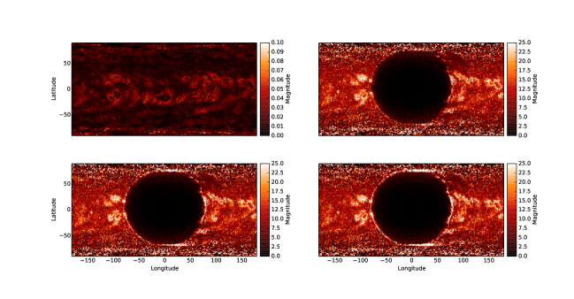
Figure 1: ADAPT Standard Deviation Frames: In each of the above frames the pixel-by-pixel standard deviation of the analysis ensemble for different ensemble Kalman filtering methods is shown; ETKF (top left), LETKF with $\rho=1.5$ (top right), LETKF with $\rho=2.0$ (bottom left), LETKF with $\rho=2.5$ (bottom right). All frames represent the same time in an ADAPT assimilation run using the same SOLIS-VSM observations. Namely, the data being assimilated were observed from SOLIS-VSM on 26 September 2003 at 16:51. We can see the drastic reduction in pixel-wise ensemble variance under the ETKF scheme. Also, an artifact of the ensemble inflation under the LETKF scheme is noticeable. Near the polar regions, observation noise (variance) is high. This causes the restriction of the pixel-wise ensemble variance under LETKF to be slight near the polar regions. Thus, the standard deviation blows up for $\rho=2.0$ and $\rho=2.5$ near these regions. This shows up as a white streak near the polar portion of the observation region in the bottom frames.

3.1 ETKF vs. LETKF

In situations, such as in solar photosphere models, where the dimension of the simulation state space is high, small ensemble size will give rise to spurious correlations [23, 18, 43, 33, 32]. In the case of the solar photosphere these occur over long distances and thus severely restrict the analysis ensemble’s pixel-wise standard deviation both near and far away from observations (see Figure 1). On the other hand, the local ensemble transform Kalman filter (LETKF) only compares each pixel’s observation with a model ensemble of pixels nearby, as described above. This eliminates the propagation of strong correlations over long distances due to the small ensemble size. We can see in Figure 1 that the pixel-wise standard deviation is only severely restricted in the interior of the observation region.

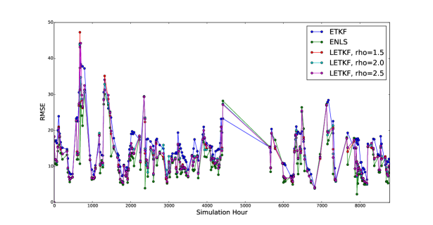
Figure 2: Forecast RMSE over observation region: Here we show the time series of the average root mean square error (RMSE) between the forecast mean and the observation using each of the data assimilation methods available in ADAPT. The time period for this time series is between 26 September 2003 and 26 September 2004. The average is taken over each pixel in the observation region. This figure shows that, in terms of RMSE, none of the data assimilation methods outperforms the others in the RMSE metric consistently over the period studied. However, RMSE is not the only method of distinguishing the usefulness of the data assimilation methods.

The main effect of the variance reduction, in terms of accuracy of the data assimilation, is how much the observations are taken into account when adjusting the photosphere ensemble. The contrast is highlighted by observing one assimilation step for a large active region using the two methods, as seen in Figure 3. The mean shape of the active region is almost unaffected by the observations for the ETKF but is noticeably influenced by observations when the LETKF is utilized.

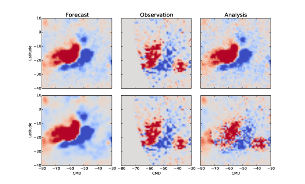
Figure 3: Comparison of ETKF and LETKF assimilation effects: The top row represents one step of the ETKF assimilation. The Bottom row is one step of the LETKF assimilation. The first column is the mean forecast, second column is the observation, and the last column is the analyzed ADAPT ensemble mean. We can see that the ETKF essentially ignores the observation while the LETKF blends the observation and forecast ensemble. The data being assimilated were observed from SOLIS-VSM on 26 September 2003 at 16:51.

3.2 ENLS vs. LETKF

The ensemble least squares (ENLS) data assimilation that ADAPT has used in the past [4] suffers from the opposite problems to those that hinder the ETKF. Briefly, the ENLS method [7] updates each ensemble member pixel-by-pixel using the formula

$$x_{a}=x_{\mathrm{f}}+\frac{\sigma_{\mathrm{f}}^{2}}{\sigma_{\mathrm{f}}^{2}+\sigma_{\textrm{obs}}^{2}}(y_{\textrm{obs}}-x_{\mathrm{f}}),$$ (3.1)

where $x_{\mathrm{f}}$ is a pixel value of the ensemble member being updated, $y_{\textrm{obs}}$ is the observed value for that pixel, $\sigma_{\mathrm{f}}$ is the ensemble standard deviation for the pixel, $\sigma_{\textrm{obs}}$ is the observation noise standard deviation, and $x_{a}$ is the analyzed ensemble pixel value. In the ENLS scheme a pixel in the ensemble is only updated if there exists a direct observation of its value. With the ENLS, observations are assimilated into the ADAPT ensemble pixel by pixel without taking sampled spatial correlations into account. Only pixel-wise standard deviations are considered, resulting in local distortion of coherent structures, such as large active regions, in the photospheric magnetic flux present in the ensemble. This is due to noise in magnetic flux observations that is not spatially correlated and therefore reduces spatial correlations in the observation.

Overall the result of the ENLS data assimilation is to assign a much greater weight to the observations than the model. This reduces the information gained by including the Worden–Harvey model for photospheric flux transport. By observing one assimilation step, for the same active region portrayed in Figure 3, we can see how the ENLS favors the observed magnetic flux more than the ADAPT ensemble model structure. In Figure 4 the ENLS data assimilation step drastically modifies the shape of the active region in its analysis ensemble whereas the LETKF blends the information from the Worden–Harvey model and the observations, maintaining the structure of the active region.

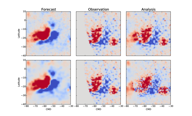
Figure 4: Comparison of ENLS and LETKF assimilation effects: Top row represents one assimilation step using ENLS, while the bottom row utilizes LETKF. The first column is the mean forecast, second column is the observation, and the last column is the analyzed ADAPT ensemble mean. The ENLS algorithm performs a pixel-by-pixel assimilation and therefore ignores spatial correlations in the ensemble. This leads to discarding the ADAPT ensemble forecast in favor of the observations. Since the LETKF takes into account local spatial correlations, large structures, such as this active region, are better preserved. The data being assimilated were observed from SOLIS-VSM on 26 September 2003 at 16:51.

4 Discussion

Three different varieties of ensemble Kalman filtering have been compared for use as data assimilation methodologies in forecasting the global solar photospheric magnetic flux. Each of these methods treated the flux transport covariance structure differently, and we showed that this led to drastically different effects. Although the ensemble Kalman methods have been studied in the context of solar weather before [27, 10, 12] the use of a physical model combined with real solar observations in the application to the photosphere is new. Moreover, we have highlighted the importance of considering spatial covariance in such data assimilation schemes and being wary of relying on a global covariance structure estimated by sampled ensemble members.

The current ADAPT framework, using the LETKF implementation in the LANL data assimilation module, does a noticeably better job at balancing the spatial propagation of information away from the point of observation. Ensemble Kalman filtering, as opposed to ensemble least squares filtering, also preserves the variance in the ensemble near data much more. This allows for a more diffuse model forecast in regions where observations have not yet been made, which increases the chance of the ensemble range capturing the true photospheric flux in these regions.

At the same time, a problem in photosphere forecasting noted previously [46, 30] is loss of balance in magnetic flux when assimilating large solar active regions on the boundary of the observation region. When this happens, the observations observe only one polarity of what should be a coupled polarity active region. Since the WH model does not include active region creation, for emerging active regions the ADAPT ensemble cannot have members that include the opposite polarity region outside of the observation domain [46].

In the near future, we plan to incorporate farside estimates of newly emerged strong magnetic regions (that is, regions not directly observed from the Earth-side of the Sun) into the ADAPT model. A preliminary example of utilizing farside data within ADAPT is highlighted by [2]. Estimates of the magnetic field strength and area of farside active regions are possible with the helioseismic acoustic holography technique [[, e.g.]]LindseyBraun1997. The measured helioseismic farside phase delay values have been parameterized in terms of photospheric magnetic field strength [17], allowing for an estimation of new solar magnetic activity on the solar farside while updating the Earth-side of global synoptic maps. The practical application of the farside data has recently been discussed with regards to space weather parameter forecasting, for example solar wind [2], F_10.7 [22, 17] and Lyman-$\alpha$ irradiance [15].

A further improvement that we plan on pursuing for ADAPT is to incorporate smooth spatial damping of correlations in the local data assimilation regions for observations farther from the pixel being analyzed [16]. In the current LETKF implementation, observations on the boundary of the local ellipse have the same weight as observations over the pixel being analyzed. This is known to cause discontinuities along the edge of the local data assimilation region [24, 45]. By adding a distance-dependent weighting to the observations within the local ellipse this problem can be eliminated.

The ADAPT photospheric forecasting capability continues to improve. This will lead to more timely boundary conditions for coronal and solar wind models which drive near Earth space weather forecasting. The data assimilation portion of the ADAPT framework now has the ability to preserve ensemble variance near observations as well as far from observations. This enables a more realistic probable range of predictions. However, to notice this improvement one must be sure to consider the structure of the entire ensemble forecast as opposed to only comparing the ensemble mean with observed data.

References

- [1] Vasilis Archontis. Magnetic flux emergence in the sun. J. Geophys. Res.: Space Physics (1978–2012), 113(A3), 2008.
- [2] C Nick Arge, Carl J Henney, I. González Hernández, W Alex Toussaint, Josef Koller, and Humberto C Godinez. Modeling the corona and solar wind using ADAPT maps that include far-side observations. In Gary P. Zank, Joe Borovsky, Roberto Bruno, Jonathan Cirtain, Steve Cranmer, Heather Elliott, Joe Giacalone, Walter Gonzalez, Gang Li, Eckart Marsch, Ebehard Moebius, Nick Pogorelov, Jim Spann, and Olga Verkhoglyadova, editors, SOLAR WIND 13: Proceedings of the Thirteenth International Solar Wind Conference, volume 1539, pages 11–14, Big Island, Hawaii, 2013. AIP.
- [3] C Nick Arge, Carl J Henney, Josef Koller, C Rich Compeau, Shawn Young, David MacKenzie, Alex Fay, and John W Harvey. Air force data assimilative photospheric flux transport (ADAPT) model. In M. Maksimovic, K. Issautier, N. Meyer-Vernet, M. Moncuquet, and F. Pantellini, editors, Twelfth International Solar Wind Conference, volume 1216, pages 343–346, Saint–Malo, France, 2010. AIP.
- [4] CN Arge, CJ Henney, J Koller, WA Toussaint, JW Harvey, and S Young. Improving data drivers for coronal and solar wind models. In Nikolai V. Pogorelov, editor, ASTRONUM–2010, volume 444, page 99, San Francisco, CA, 2011. Astron. Soc. Pac.
- [5] Eric Bélanger, Alain Vincent, and Paul Charbonneau. Predicting solar flares by data assimilation in avalanche models. Solar Phys., 245(1):141–165, 2007.
- [6] Craig H Bishop, Brian J Etherton, and Sharanya J Majumdar. Adaptive sampling with the ensemble transform kalman filter. part I: Theoretical aspects. Monthly weather review, 129(3):420–436, 2001.
- [7] F Bouttier and P Courtier. Data assimilation concepts and methods March 1999. Meteorological training course lecture series, 2002.
- [8] Allan Sacha Brun. Towards using modern data assimilation and weather forecasting methods in solar physics. Astron. Nach., 328(3-4):329–338, 2007.
- [9] Allan Sacha Brun and Laurene Jouve. Global models of the magnetic sun. Proc. Int. Astron. Un., 3(S247):33–38, 2007.
- [10] MD Butala, RJ Hewett, RA Frazin, and F Kamalabadi. Dynamic three-dimensional tomography of the solar corona. Solar Phys., 262(2):495–509, 2010.
- [11] R. Daley. Atmospheric Data Analysis. Cambridge University Press, Cambridge, 1991.
- [12] M Dikpati, J Anderson, and D Mitra. Ensemble Kalman filter data assimilation in a Babcock-Leighton solar dynamo model: An observation system simulation experiment for reconstructing meridional flow speed. Geophys. Res. Lett., 41(15), 2014.
- [13] M Dikpati and P Gilman. Simulating and predicting solar cycles using a flux-transport dynamo. Astrophys., 649(1), 2006.
- [14] Geir Evensen. Data assimilation: The ensemble Kalman filter. Springer, New York, 2009.
- [15] J. M. Fontenla, E. Quémerais, I. González Hernández, C. Lindsey, and M. Haberreiter. Solar irradiance forecast and far-side imaging. Adv. Space Res., 44(457), 2009.
- [16] Gregory Gaspari and Stephen E Cohn. Construction of correlation functions in two and three dimensions. Quart. Roy. Met. Soc., 125(554):723–757, 1999.
- [17] I. González Hernández, M. Díaz Alfaro, K. Jain, W. K. Tobiska, D. C. Braun, F. Hill, and F. Pérez Hernández. A full-Sun magnetic index from helioseismology inferences. Solar Phys., 289(503), 2014.
- [18] Thomas M Hamill, Jeffrey S Whitaker, and Chris Snyder. Distance-dependent filtering of background error covariance estimates in an ensemble kalman filter. Mon. Weather Rev., 129(11):2776–2790, 2001.
- [19] JW Harvey, F Hill, RP Hubbard, JR Kennedy, JW Leibacher, JA Pintar, PA Gilman, RW Noyes, J Toomre, RK Ulrich, et al. The global oscillation network group (GONG) project. Science, 272:1284–1286, 1996.
- [20] David H Hathaway and Lisa Rightmire. Variations in the sun’s meridional flow over a solar cycle. Science, 327(5971):1350–1352, 2010.
- [21] CJ Henney, CU Keller, JW Harvey, MK Georgoulis, NL Hadder, AA Norton, N-E Raouafi, and RM Toussaint. Solis vector spectromagnetograph: status and science. In Svetlana V. Berdyugina, K. N. Nagendra, and Renzo Ramelli, editors, Solar Polarization–5, volume 405, page 47, Ascona, Switzerland, 2009. Astron. Soc. Pac.
- [22] CJ Henney, WA Toussaint, SM White, and CN Arge. Forecasting f10. 7 with solar magnetic flux transport modeling. Space Weather, 10, 2012.
- [23] Peter L Houtekamer and Herschel L Mitchell. A sequential ensemble kalman filter for atmospheric data assimilation. Mon. Weather Rev., 129(1):123–137, 2001.
- [24] Brian R Hunt, Eric J Kostelich, and Istvan Szunyogh. Efficient data assimilation for spatiotemporal chaos: A local ensemble transform kalman filter. Physica D: Nonlinear Phenomena, 230(1):112–126, 2007.
- [25] Laurène Jouve, Allan Sacha Brun, and Olivier Talagrand. Assimilating data into an dynamo model of the sun: a variational approach. Astrophys. J., 735(1):31, 2011.
- [26] Eugenia Kalnay. Atmospheric modeling, data assimilation, and predictability. Cambridge University Press, Cambridge, 2003.
- [27] I Kitiashvili and AG Kosovichev. Application of data assimilation method for predicting solar cycles. Astrophys. J. Lett., 688(1):L49, 2008.
- [28] RW Komm, RF Howard, and JW Harvey. Rotation rates of small magnetic features from two-and one-dimensional cross-correlation analyses. Solar Phys., 145(1):1–10, 1993.
- [29] C Lindsey and DC Braun. Helioseismic holography. Astrophys. J., 485:895, 1997.
- [30] Duncan Mackay and Anthony Yeates. The sun’s global photospheric and coronal magnetic fields: Observations and models. Living Rev. Solar Phys., 9:6, 2012.
- [31] James Marshall Mosher. The magnetic history of solar active regions. PhD thesis, California Institute of Technology, 1977.
- [32] Edward Ott, Brian R Hunt, Istvan Szunyogh, Aleksey V Zimin, Eric J Kostelich, Matteo Corazza, Eugenia Kalnay, DJ Patil, and James A Yorke. A local ensemble kalman filter for atmospheric data assimilation. Tellus A, 56(5):415–428, 2004.
- [33] Edward Ott, DJ Patil, E Kalnay, Matteo Corazza, I Szunyogh, BR Hunt, and James A Yorke. Exploiting local low dimensionality of the atmospheric dynamics for efficient ensemble kalman filtering. Technical report, 2002.
- [34] P Riley. An alternative interpretation of the relationship between the inferred open solar flux and the interplanetary magnetic field. Astrophys. J., 667, 2007.
- [35] J Schou, PH Scherrer, RI Bush, R Wachter, S Couvidat, MC Rabello-Soares, RS Bogart, JT Hoeksema, Y Liu, TL Duvall, et al. Design and Ground Calibration of the Helioseismic and Magnetic Imager (HMI) Instrument on the Solar Dynamics Observatory (SDO). Solar Phys., 275:229–259, 2012.
- [36] Carolus J Schrijver and Title M Alan. On the formation of polar spots in sun-like stars. Astrophys. J., 551(2):1099, 2001.
- [37] GW Simon, AM Title, and NO Weiss. Kinematic models of supergranular diffusion on the sun. Astrophys., 442:886–897, 1995.
- [38] Herschel B Snodgrass. Magnetic rotation of the solar photosphere. Astrophys. J., 270:288–299, 1983.
- [39] Dennis G Socker, Russell A Howard, Clarence M Korendyke, George M Simnett, and David F Webb. NASA Solar Terrestrial Relations Observatory (STEREO) mission heliospheric imager. In Silvano Fineschi, Clarence M. Korendyke, Oswald H. W. Siegmund, and Bruce E. Woodgate, editors, Instrumentation for UV/EUV Astronomy and Solar Missions, page 284, San Diego, CA, 2000. Intern. Soc. Opt. Photo.
- [40] Andreas Svedin, Milena C Cuéllar, and Axel Brandenburg. Data assimilation for stratified convection. Mon. Not. Roy. Astron. Soc., page 891, 2013.
- [41] Xuguang Wang and Craig H Bishop. A comparison of breeding and ensemble transform kalman filter ensemble forecast schemes. J. Atmos. Sci., 60(9):1140–1158, 2003.
- [42] Y-M Wang and NR Sheeley. The rotation of photospheric magnetic fields: A random walk transport model. Astrophys. J., 430:399–412, 1994.
- [43] Jeffrey S Whitaker and Thomas M Hamill. Ensemble data assimilation without perturbed observations. Mon. Weather Rev., 130(7):1913–1924, 2002.
- [44] John Worden and John Harvey. An evolving synoptic magnetic flux map and implications for the distribution of photospheric magnetic flux. Solar Phys., 195(2):247–268, 2000.
- [45] Shu-Chih Yang, Eugenia Kalnay, Brian Hunt, and Neill E Bowler. Weight interpolation for efficient data assimilation with the local ensemble transform kalman filter. Quart. Roy. Met. Soc., 135(638):251–262, 2009.
- [46] Anthony R Yeates, Dibyendu Nandy, and Duncan H Mackay. Exploring the physical basis of solar cycle predictions: flux transport dynamics and persistence of memory in advection-versus diffusion-dominated solar convection zones. Astrophys. J., 673(1):544, 2008.
- [47] Jie Zhang, Yuming Wang, and Yang Liu. Statistical properties of solar active regions obtained from an automatic detection system and the computational biases. Astrophys. J., 723(2):1006, 2010.